Retrieval of Snow Depths on Arctic Sea Ice in the Cold Season from FY-3D/MWRI Data

Abstract

Snow depth is a crucial factor in the formation of snow, and its fluctuations play a significant role in the Earth’s climate system. The existing snow depth algorithms currently lack systematic quantitative evaluation, and most of them are not suitable for direct application to Chinese satellites. Therefore, a quantitative evaluation of four existing snow depth algorithms from the Advanced Microwave Scanning Radiometer 2 (AMSR2) was conducted by comparing their estimates with the measured dataset from the Operation IceBridge project (OIB). The study found that the algorithm developed by Rostosky et al. outperforms the other three algorithms in terms of correlation. However, it is unable to accurately retrieve both high and low snow depths. On the other hand, the algorithms developed by Comiso et al. and Li et al. demonstrated strong performance in correlation and statistical characteristics. Based on these results, these two algorithms were fused to enhance the accuracy of the final algorithm. The algorithm was applied to FengYun-3D/Microwave Radiation Imager (FY-3D/MWRI) data after calibration to develop a snow depth retrieval algorithm suitable for MWRI. Validation using the 2019 OIB data indicated that the algorithm had a bias and RMSE of 1 cm and 9 cm, respectively, for first-year ice (FYI) and 3 cm and 9 cm, respectively, for multi-year ice (MYI).

1. Introduction

The Arctic is one of the regions most vulnerable to global climate change, as it experiences a warming rate approximately 1.5–4.5 times higher than the global average [1]. This is due to its unique environment, which amplifies the impacts of climate change [2]. The presence and changes in the primary environmental factors in the Arctic, such as ice and snow, have profoundly influenced the climate, hydrology, and ecology of the polar region, as well as the global environment. Snow on ice effectively reduces the heat exchange between ice and air due to its lower heat conductivity, which is about one-tenth that of sea ice [3]. The attenuation of solar radiation is closely related to snow. The impact of attenuation is 100 times greater than that of sea ice of the same thickness [4,5]. In addition, the melting and growth of sea ice are also influenced by snow [6].

The depth of snow is a crucial factor in accurately estimating snowfall, precipitation, and freshwater output [7]. The accuracy of estimating snow depth can directly impact the calculation of sea ice thickness and volume. Reliable estimation of snow depth can offer deeper insights into the spatiotemporal changes in Arctic sea ice and aid in studying the heat exchange in the Arctic [8]. Although it is crucial to investigate snow depth on ice, the datasets derived from in situ or satellite measurements are still insufficient [9]. In 2013, the fifth assessment report of the Intergovernmental Panel on Climate Change (IPCC) [10] suggested that the examination of snow depth on the Arctic ice was an urgent issue that needed to be addressed. In 2019, the IPCC once again emphasized the significance of snow depth on ice in its special report [11].

Currently, the acquisition of data on snow depth largely relies on two major methods: in situ observations (such as on-site observations, buoy measurements, airborne measurements, et al.) and satellites. In 1937, the Arctic and Antarctic Research Institute (AARI) established its first drifting station in the Arctic to collect long-term snow depths [12]. Based on this, Warren et al. employed a binary quadratic model to successfully obtain the snow depth across the entire Arctic, resulting in the development of a monthly Arctic snow depth model (W99) [13]. Due to the constraints in the location of drift stations, the model has a limitation of inadequate accuracy in retrieving the snow depth on FYI. This model is based on data from the last century, and it is uncertain if it can accurately predict the current snow depth. Furthermore, daily and annual changes have not been considered in the model.

The implementation of the Arctic Ocean Buoy Project in 1979 enabled the detection of snow depth on sea ice using buoys [14]. In recent years, the Cold Regions Research and Engineering Laboratory in the United States has released the Ice Mass Balance snow depth dataset (IMB) as a data source for snow depth assessment in the Arctic. It began in 1993, providing a large number of high-precision measurement point datasets, and due to the acquisition method of buoys, unmanned observation has been achieved to a certain extent. OIB was implemented in 2009 to measure polar parameters in spring, and the snow depth was obtained using a snow radar, which also provides strong and reliable support for snow information on the ice as well as for the inversion of snow depth.

However, due to environmental constraints, measured data alone cannot provide large-scale and long-term continuous observations. Therefore, the usage of satellite datasets to invert the snow depth on the Arctic sea ice is of great significance for studying changes in Arctic snow. Markus and Cavalieri investigated the correlation between brightness temperature at different channels based on the Special Sensor Microwave Imager (SSM/I) and Antarctic cruise data and proposed a retrieval model using 37 GHz and 19 GHz, which led to the development of the first passive microwave remote sensing algorithm for snow depth inversion [15]. This model was further developed by several researchers, and its parameters were modified to retrieve data using different microwave sensors [16,17]. For example, the snow depth inversion algorithm (Co03) of Advanced Microwave Scanning Radiometer for EOS (AMSR-E) and the snow depth inversion algorithm of MWRI. However, the emission characteristics of MYI are similar to those of deep snow at specific frequencies. Li et al. combined the MEMLS model to investigate the brightness temperature gradient ratio (GR) on snow. They concluded that the GR (19 V/37 V) decreased in FYI and tended to saturate when the snow depth was above 50 cm, while the snow depth on MYI was 30 cm. Under the conditions of wet snow, the radiative ratio of 19 GHz and 37 GHz is close to 1, and the GR is close to 0 [18]. Therefore, the algorithm is only applicable to dry snow on FYI with a snow depth of less than 50 cm. To overcome these limitations, Markus et al. proposed the idea of using low-frequency channels to improve the ability of the snow depth retrieval from the passive microwave, thus supporting the acquisition of snow depth on the MYI [19]. Based on this assumption, Rostosky et al. compared the OIB dataset to the AMSR-E data and developed a snow depth inversion model using AMSR2 at 7 GHz and 19 GHz for the creation of a snow depth inversion algorithm for the entire Arctic (Ro18) [20]. Li et al. adopted similar methods to process the MWRI data and developed snow depth inversion algorithms based on 19 GHz and 10 GHz (Li_MWRI) [18]. He et al. combined Soil Moisture Active Passive (SMAP) and AMSR2 data to explore snow depth based on 1 GHz and 19 GHz [21]. However, as the OIB data only includes snow depth measurements of spring, it performs poorly in autumn and winter. When compared with OIB data, the IMB dataset provides a longer time series of snow depth data and has emerged as one of the reliable datasets for comparison and investigation of snow depth. Furthermore, as this dataset covers the entire year, it can be effectively utilized for developing inversion algorithms for other seasons. Further, Kilic et al., Liu et al., and Li et al. compared it with AMSR2 data and developed a robust algorithm for retrieving snow depth on Arctic Sea ice (Ki19 and Li22) [22,23,24].

Although various methods have been employed to estimate the snow depth on Arctic sea ice, there are still notable discrepancies in the results produced by different algorithms, particularly when it comes to snow on MYI. Currently, only a few algorithms are suitable for China’s satellites. Furthermore, because of variations in channel configuration among different sensors, it is challenging to apply most algorithms directly. The inversion of snow depth on MYI depends on low-frequency bands. However, some Chinese satellites have not been equipped with this capability, leading to inadequacies in retrieving snow depth on MYI based on Chinese satellites. Therefore, it is crucial to enhance existing algorithms and develop a snow depth retrieval algorithm suitable for Chinese satellites. This will contribute to a better understanding and exploration of the polar regions. In this study, four algorithms suitable for AMSR2 were selected and compared with OIB data. Based on the comparison results, specific enhancements have been integrated into the algorithm. Furthermore, both MWRI data and AMSR2 data were used to develop an Arctic snow depth inversion algorithm suitable for MWRI.

2. Study Area and Data

2.1. Study Area

According to the geographic definition, the Arctic covers a vast sea in the north of the Arctic Circle. Due to the orbit inclination (98.75° in FY-3D), the study area is confined to 66°N–88°N. According to the National Snow and Ice Data Center (NSIDC), the Arctic includes 10 sub-regions, namely, Beaufort Sea, Chukchi Sea, East Siberian Sea, Laptev Sea, Kara Sea, Barents Sea, East Greenland Sea, Baffin Bay and Davis Strait, Canadian Archipelago, and Central Arctic (Figure 1a).

2.2. Data

2.2.1. Brightness Temperature

In this study, two sets of brightness temperature data were considered: MWRI L1 datasets with a spatial resolution of 10 km and AMSR2 L3 datasets with a spatial resolution of 25 km. The MWRI is deployed on the Meteorological Satellite FY-3 and is one of the ten major detection instruments on the FY-3D. It can provide global observations of brightness at five frequencies ranging from 10 to 89 GHz (10.65 GHz, 18.7 GHz, 23.8 GHz, 36.5 GHz, and 89 GHz). Each frequency contains two polarization modes (horizontal polarization H and vertical polarization V), ultimately forming 10 channels. The scanning mode uses conic scanning with a width of 1400 km. The Advanced Microwave Scanning Radiometer 2 (AMSR2) is installed on the Global Change Observation Mission 1st-Water (GCOM W1) satellite, which was launched by the Japan Aerospace Exploration Agency (JAXA). The brightness temperature dataset from AMSR2 covers seven frequencies ranging from 6 to 89 GHz using the same scanning mode. It can provide global precipitation, water vapor content, snow depth, and other relevant datasets (

Table 1. Specifications of the MWRI and AMSR2 channels.

	Channel/GHz	6.925	7.3	10.65	18.7	23.8	36.5	89
MWRI	Polarization	-	-	V.H	V.H	V.H	V.H	V.H
	Spatial resolution/km	-	-	51 × 85	30 × 50	27 × 45	18 × 30	9 × 15
AMSR2	Polarization	V.H	V.H	V.H	V.H	V.H	V.H	V.H
	Spatial resolution/km	62 × 35	62 × 35	42 × 24	22 × 14	19 × 11	12 × 7	5 × 3

).

2.2.2. Sea Ice Type

The emission characteristics differ between FYI and MYI; therefore, it is necessary to differentiate them during the investigation of snow depth. As one of the mature sea ice products in the Arctic, sea ice type products have been widely used in polar snow research. To make a distinction between ice types, the data product on sea ice type provided by the Satellite Application Facility on Ocean and Sea Ice (OSI SAF) was employed in this study. Based on the Bayesian multi-sensor method, the type is obtained using the multi-sensor and auxiliary data. The Bayesian method describes the probability of the most likely surface classes occurring. Therefore, the final surface class in the mesh points is defined as the class with the highest probability. It can provide the daily dataset on types of sea ice across the entire Arctic with a spatial resolution of 10 km (Figure 1b) and is categorized into three types: FYI (blue), MYI (green), and ambiguous type (yellow).

2.2.3. Sea Ice Concentration

The daily sea ice concentration (SIC) product was derived from brightness temperature datasets by selecting specific sensors. It can provide SIC data for the entire Arctic (Figure 2a,b). Different algorithms were used to obtain the data, resulting in different values (especially in the edge area). The ARTIST (Arctic Radiation and Turbulence Interaction Study) Sea Ice algorithm (ASI) was used to obtain SIC from AMSR2, whereas the enhanced NASA Team algorithm (NT2) was used in the case of MWRI. Further, the spatial resolution is not the same for both datasets. The resolution of AMSR2 and MWRI were 6.25 km and 12.5 km, respectively.

2.2.4. Sea Ice Snow Depth Reference Datasets

In 2009, the National Aeronautics and Space Administration (NASA) launched the OIB mission, which lasted for 11 years. The mission employed airborne radar to carry out a series of land and ice detections to fill data gaps between Ice, Cloud, and land Elevation Satellite (ICESat) and ICESat-2 missions. Compared to the IMB, OIB data are closer to the satellite footprint, increasing the consistency with the satellite observations. The project generated a large dataset of airborne measured snow depth, and quality control was applied, with a mean bias of about −5 cm [25], which was instrumental in the evaluation of inversion results. The airborne measured data (snow depth) from 2013 to 2019 (Figure 2c) was used in this study to improve the accuracy of the results.

W99m was developed using the climatology snow depth dataset of W99, and it includes five major areas, namely, Beaufort Sea, Chukchi Sea, East Siberian Sea, Laptev Sea, and Central Arctic (Figure 2d). This dataset retains the snow depth in W99 for MYI and uses half of the dataset for FYI based on Laxon’s suggestion [26]. This adjustment significantly enhanced the accuracy of the snow depth in FYI. However, due to the limitations of W99, this dataset cannot accurately represent the snow depth in the Arctic. Especially in recent years, with the decline in snow depth caused by climate warming, the overestimation resulting from this dataset was becoming increasingly serious year by year [9]. According to the comparative results of W99m and satellite inversion datasets (AMSR2, FY-3B/MWRI, MW99/AMSR2) by Zhou et al., the W99m showed higher values (0.04 m, 0.06 m, and 0.04 m in winter, respectively) [27]. However, it can still be utilized to estimate snow depth due to the wide distribution of the measured data used for fitting across seasons.

In addition, Li et al. developed an Arctic snow depth model (Equations (1) and (2)) for FY-3B/MWRI based on the MEMLS model and OIB-measured dataset [20]. This algorithm is capable of retrieval of the snow depth on the sea ice of the entire Arctic during the cold season, and it is the first algorithm of snow depths from MWRI that realizes the full coverage of the Arctic sea ice. However, since the algorithm is primarily designed for FY-3B, the results were not directly applied in this paper but were calculated.

$$H_{s_{\_FYI}}=54.45-703.41\times \frac{tb\left(19 \mathrm{V}\right)-tb\left(7 \mathrm{V}\right)}{tb\left(19 \mathrm{V}\right)+tb\left(7 \mathrm{V}\right)}-0.17\times tb\left(37 \mathrm{V}\right)$$

(1)

$$H_{s_{\_FYI}}=295.15-568.58\times \frac{tb\left(19 \mathrm{V}\right)-tb\left(7 \mathrm{V}\right)}{tb\left(19 \mathrm{V}\right)+tb\left(7 \mathrm{V}\right)}+0.41\times tb\left(10 \mathrm{V}\right)-1.52\times tb\left(19 \mathrm{V}\right)$$

(2)

where, $H_{s_{\_FYI}}$ and $H_{s_{\_MYI}}$ represent the snow depths on MYI and FYI, respectively, $tb\left(37 \mathrm{V}\right)$, $tb\left(19 \mathrm{V}\right)$, $tb\left(10 \mathrm{V}\right)$ and $tb\left(7 \mathrm{V}\right)$ represent the brightness temperatures of 37 V, 19 V, 10 V, 7 V, respectively.

To sum up, this paper utilized two types of datasets and an algorithm as reference datasets. The measured data (OIB) was valuable for enhancing the algorithm and verifying the data due to its high accuracy. On the other hand, W99m was solely employed to assess the algorithm’s seasonal adaptability, as it has limitations and was not utilized as a standard for quantitative evaluation. The Li_MWRI was used for parallel comparison to demonstrate the algorithm’s reliability in snow depth.

In order to ensure the consistency of spatial resolution in processing, the projection method of W99m dataset was used as the benchmark, the spatial interpolation method was used to unify the above-mentioned datasets into NSIDC Sea Ice Polar Stereographic North of 25 km (EPSG: 3413), and resampling, minimum-distanced matching and mean value method were combined to obtain the brightness temperature in the Arctic of 25 km polar stereoscopic projection coordinate system, and the region with less than 0.15 SIC was removed.

3. Method

3.1. Several Snow Depth Inversion Algorithms

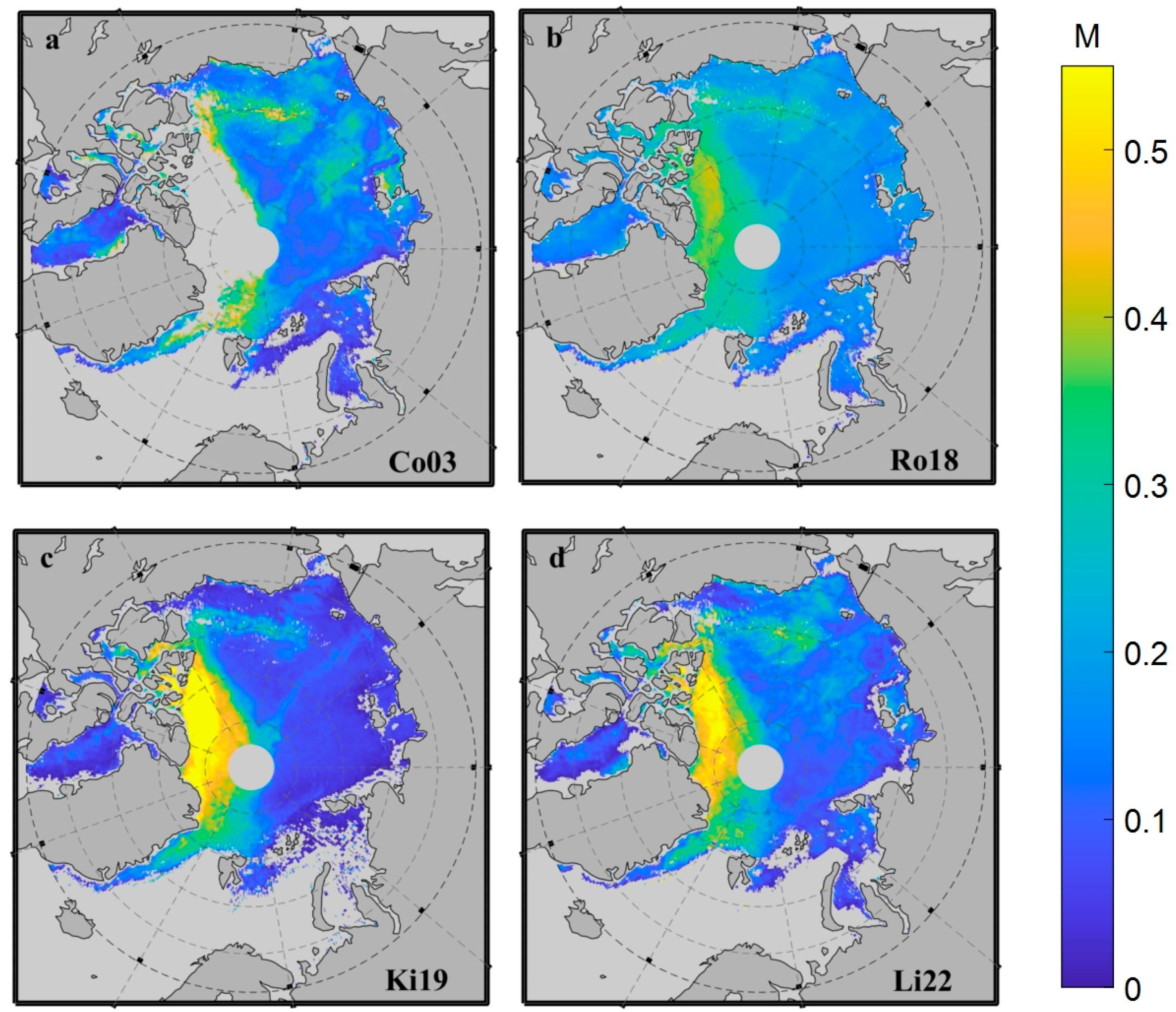
As mentioned in the earlier section, there is a high similarity in the configuration of channels with MWRI, and several snow depth algorithms have been developed using AMSR2. In order to develop the final snow depth inversion algorithm using MWRI TB, this paper aimed to enhance the existing AMSR2 algorithm for its adaptation to MWRI. Therefore, to further investigate these algorithms’ performance, four snow depth inversion algorithms of AMSR2 (Co03, Ro18, Ki19, and Li22) were selected (Figure 3), and their accuracy was evaluated. The daily snow depth products were generated based on the brightness temperature dataset and SIC product of AMSR2 and the accuracy was verified using the OIB-measured dataset.

A brief introduction to each algorithm is provided below.

3.1.1. Co03

Markus and Cavalieri reported the correlation between Antarctic cruise data and brightness temperature, brightness temperature difference, and the SSMI spectral gradient information [15]. It was observed that a higher correlation (−0.77) and a smaller standard deviation (7.8 cm) can be achieved using the spectral gradient ratio from channels 19 V and 37 V. Based on the data fitting, a snow depth inversion algorithm suitable for polar was obtained. Based on this, Comiso et al. further processed AMSR2 data to obtain the new coefficients [16]. The snow depth is calculated by Equation (3).

$$H_s=2.9-782\times \frac{t_{bice}\left(37 \mathrm{V}\right)-t_{bice}\left(19 \mathrm{V}\right)}{t_{bice}\left(37 \mathrm{V}\right)+t_{bice}\left(19 \mathrm{V}\right)}$$

(3)

$$t_{bice}\left(37 \mathrm{V}\right)=\frac{tb\left(37 \mathrm{V}\right)-\left(1-C\right)\times t_w\left(37 \mathrm{V}\right)}{C}$$

(4)

$$t_{bice}\left(19 \mathrm{V}\right)=\frac{tb\left(19 \mathrm{V}\right)-\left(1-C\right)\times t_w\left(19 \mathrm{V}\right)}{C}$$

(5)

where $H_s$ is the snow depth on Arctic sea ice, $tb\left(37 \mathrm{V}\right)$ and $tb\left(19 \mathrm{V}\right)$ represent the brightness temperatures of 37 V and 19 V, respectively, $C$ is the SIC obtained from the ASI algorithm and ranged from 0 to 1, and $t_w\left(37 \mathrm{V}\right)$ and $t_w\left(19 \mathrm{V}\right)$ represent the brightness temperature values of 37 V and 19 V in the open water, i.e., 200.5 K and 176.6 K, respectively.

As the saturation problem and the sensitivity problem, the algorithm is only suitable for dry snow on FYI with a depth of less than 50 cm. However, as this algorithm performs well on FYI, it was also considered in this study.

3.1.2. Ro18

To further explore the relevant situation of the snow depth on MYI, obtain the depth of the snow on the entire Arctic Sea ice, and improve the spatiotemporal variational characteristics of the snow depth, Rostosky et al. computed the frequency gradient ratio between the vertical polarization channels of AMSR2 and performed correlation analysis with the depth of snow on FYI and MYI measured in the OIB dataset [19]. Finally, it was observed that 19 V and 7 V had the highest correlation coefficients (−0.60 and −0.55, respectively). Thus, a new snow depth model for the entire Arctic was proposed.

$$H_{s_{\_FYI}}=19.26-553\times \frac{t_{bice}\left(19 \mathrm{V}\right)-t_{bice}\left(7 \mathrm{V}\right)}{t_{bice}\left(19 \mathrm{V}\right)+t_{bice}\left(7 \mathrm{V}\right)}$$

(6)

$$H_{s_{\_MYI}}=19.34-368\times \frac{t_{bice}\left(19 \mathrm{V}\right)-t_{bice}\left(7 \mathrm{V}\right)}{t_{bice}\left(19 \mathrm{V}\right)+t_{bice}\left(7 \mathrm{V}\right)}$$

(7)

$$t_{bice}\left(7 \mathrm{V}\right)=\frac{tb\left(7 \mathrm{V}\right)-\left(1-C\right)\times t_w\left(7 \mathrm{V}\right)}{C}$$

(8)

where, $H_{s_{\_FYI}}$ and $H_{s_{\_MYI}}$ represent the snow depths on MYI and FYI, respectively, $tb\left(7 \mathrm{V}\right)$ indicates the brightness temperature of 7 V, and $t_w\left(19 \mathrm{V}\right)$ and $t_w\left(7 \mathrm{V}\right)$ indicate the brightness temperature values of 19 V and 7 V in the open water, which are 183.72 K and 161.35 K, respectively [28].

Considering that the sampling duration for OIB is only from March to April (or May) each year, Rostosky et al. further evaluated the inversion results for verification of their performance in autumn and winter. However, due to the possible differences in the nature of snow during different seasons, good results were not obtained in the other seasons. This algorithm was only applicable to MYI in spring, and the algorithm on FYI can be applied for the entire cold season.

3.1.3. Ki19

To address the issue of small-time spans in OIB data, Kilic et al. applied IMB data to explore the snow depth on sea ice [22]. Due to the significant reduction in inversion accuracy of passive microwave remote sensing under high water content, Kilic et al. considered the November 1st to April 1st data in combination with the brightness temperature of AMSR2 in different channels for statistical calculations. They applied a forward regression algorithm to determine the optimal inversion frequencies for snow depth as 37 V, 19 V, and 7 V and thus developed a snow depth model for the entire Arctic.

$$H_s=1.7701+1.75\times tb\left(7 \mathrm{V}\right)-2.80\times tb\left(19 \mathrm{V}\right)+0.41\times tb\left(37 \mathrm{V}\right)$$

(9)

However, the algorithm did not fully account for the impact of open water during construction; it only considered the relevant data from IMB buoys distributed on the surface of sea ice. As a result, the accuracy of the algorithm was relatively poor in areas with low sea ice concentration (developing for areas with 100% SIC), especially in the ice-water transition zone. Therefore, Figure 3c is for presentation only.

3.1.4. Li22

Building upon the work of Rostosky et al., Li et al. made further improvements by fitting IMB data and determined that the gradient ratios of 37 H and 7 H yielded the best results for the FYI region (correlation coefficient of −0.84), while the gradient ratios of 19 V and 10 V were observed for MYI region (correlation coefficient of −0.51) [24]. Based on these two gradient ratios, an improved snow depth inversion algorithm was constructed.

$$H_{s_{FYI}}=11.01-352.17\times \frac{t_{bice}\left(37 \mathrm{H}\right)-t_{bice}\left(7 \mathrm{H}\right)}{t_{bice}\left(37 \mathrm{H}\right)+t_{bice}\left(7 \mathrm{H}\right)}$$

(10)

$$H_{s_{MYI}}=9.30-1002.20\times \frac{t_{bice}\left(19 \mathrm{V}\right)-t_{bice}\left(10 \mathrm{V}\right)}{t_{bice}\left(19 \mathrm{V}\right)+t_{bice}\left(10 \mathrm{V}\right)}$$

(11)

$$t_{bice}\left(37 \mathrm{H}\right)=\frac{tb\left(37 \mathrm{H}\right)-\left(1-C\right)\times t_w\left(37 \mathrm{H}\right)}{C}$$

(12)

$$t_{bice}\left(7 \mathrm{H}\right)=\frac{tb\left(7 \mathrm{H}\right)-\left(1-C\right)\times t_w\left(7 \mathrm{H}\right)}{C}$$

(13)

$$t_{bice}\left(10 \mathrm{V}\right)=\frac{tb\left(10 \mathrm{V}\right)-\left(1-C\right)\times t_w\left(10 \mathrm{V}\right)}{C}$$

(14)

where $tb\left(37 \mathrm{H}\right)$, $tb\left(7 \mathrm{H}\right)$ and $tb\left(10 \mathrm{V}\right)$ represent the brightness temperatures of 37 H, 7 H, and 10 V, and $t_w\left(37 \mathrm{H}\right)$, $t_w\left(7 \mathrm{H}\right)$, and $t_w\left(10 \mathrm{V}\right)$ represent the brightness temperature values of 37 H, 7 H, and 10 V in the open water, which are 145.29 K, 82.13 K, and 157.34 K, respectively [28].

3.2. Improvement in the Snow Depth Inversion Algorithm

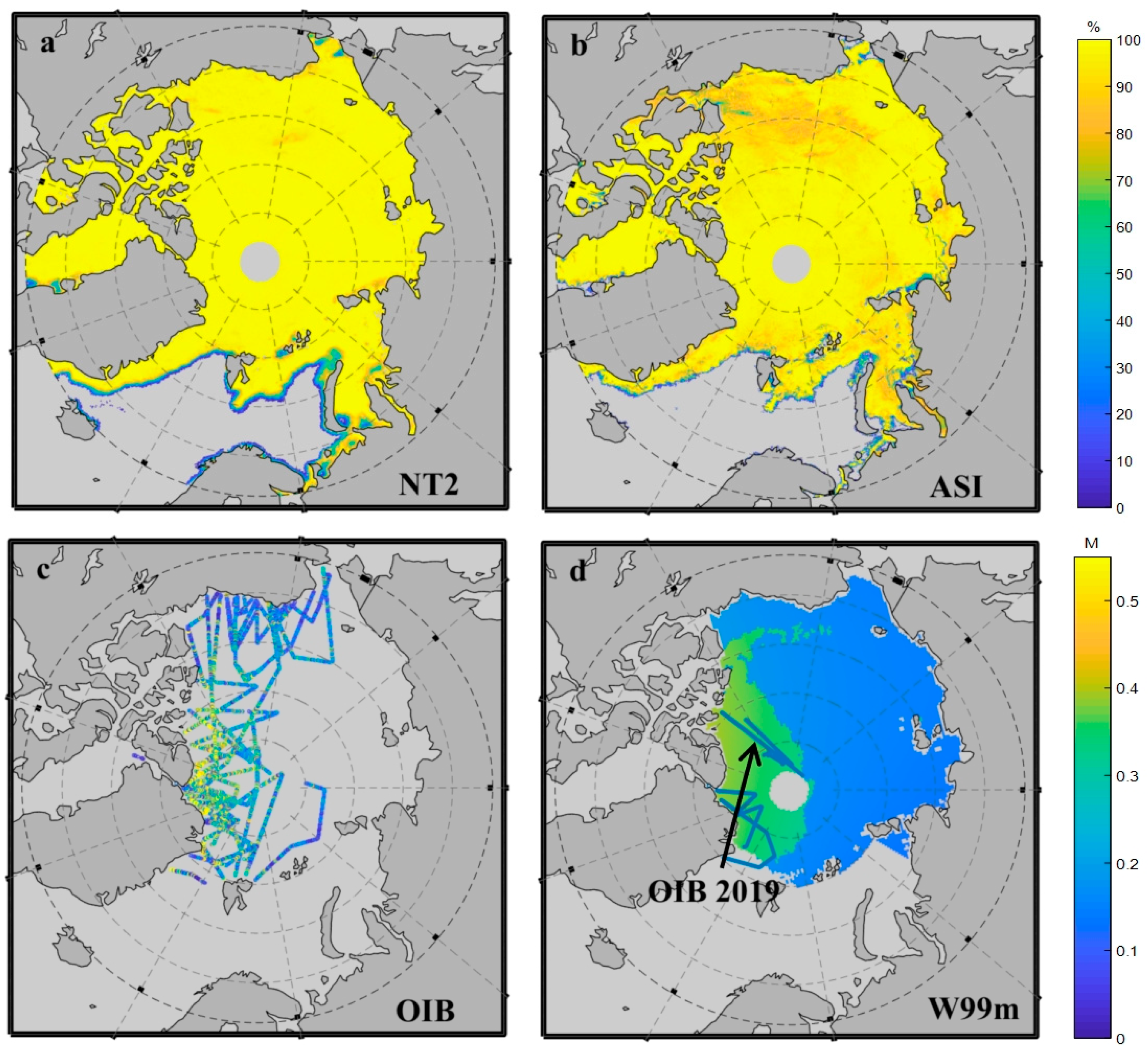
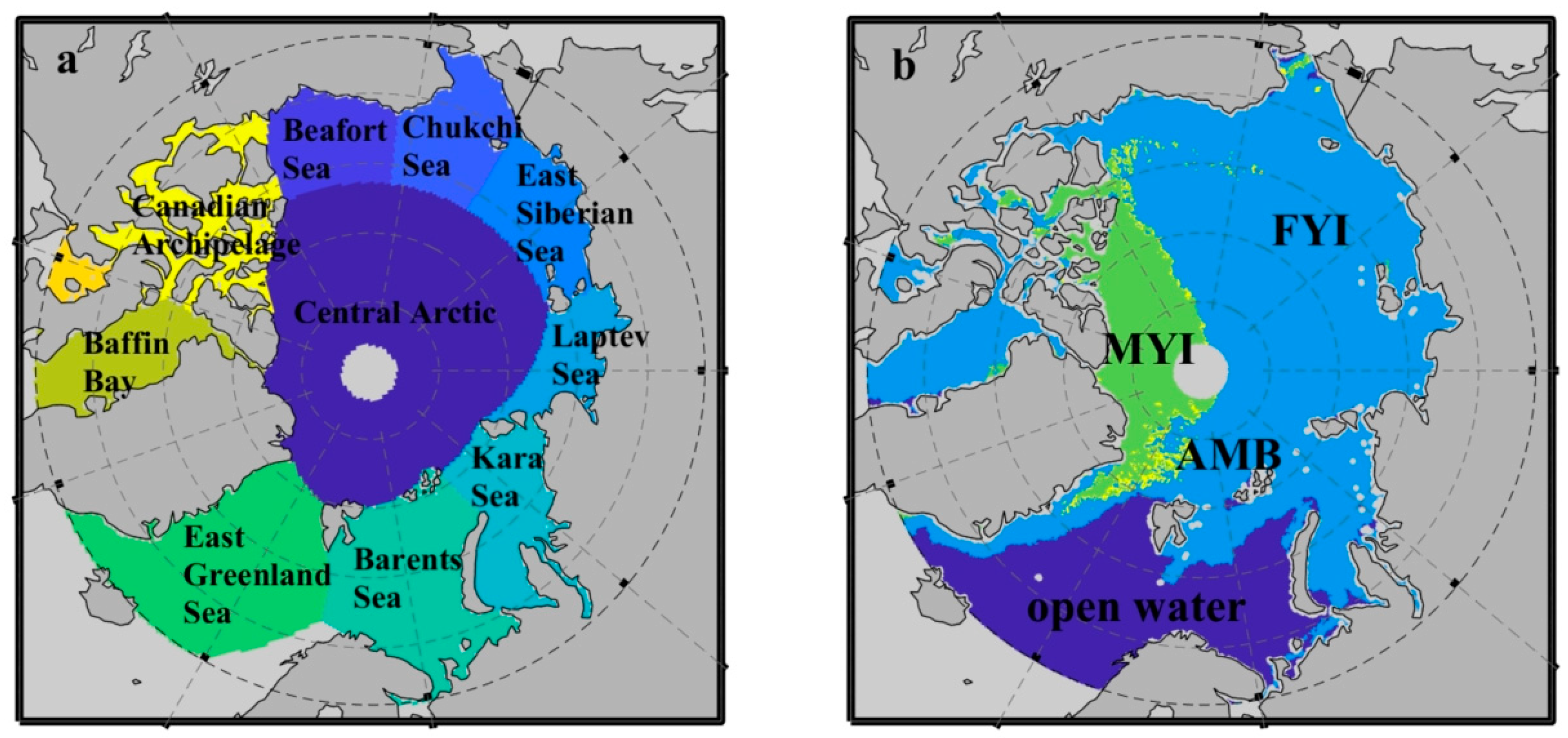
The OIB dataset from 2013 to 2019 was used to compare and validate the inversion results of the four algorithms mentioned above. Also, to avoid large errors, the OIB observation sites were averaged in a grid of 25 km × 25 km, and data with fewer than 100 statistical points in the grid were eliminated [29]. As the Co03 algorithm was unable to effectively retrieve snow depth under MYI, the sea ice type was also considered for data comparison. Apart from processing the entire Arctic, data comparison was conducted on FYI as well as MYI regions. The accuracy of the matched data was evaluated separately. The results are presented in

Table 2. Accuracy evaluations of the Co03, Ro18, Ki19, and Li22 models (using AMSR2 TB) using RMSE (m), bias (m), and correlation coefficient R based on OIB-measured snow depths (from 2013 to 2019) over MYI and FYI (in parentheses are the results for SIC = 100%).

All	Co03	Ro18	Ki19	Li22
R	-	0.61	0.60 (0.59)	0.60
RMSE/m	-	0.08	0.12 (0.12)	0.09
bias/m	-	0.00	0.02 (0.03)	0.01
FYI	Co03	Ro18	Ki19	Li22
R	0.50	0.46	0.39 (0.33)	0.45
RMSE/m	0.08	0.08	0.10 (0.10)	0.09
bias/m	0.02	0.03	−0.05 (−0.06)	−0.03
MYI	Co03	Ro18	Ki19	Li22
R	-	0.40	0.41 (0.35)	0.41
RMSE/m	-	0.09	0.12 (0.12)	0.10
bias/m	-	−0.01	0.04 (0.02)	0.02

.

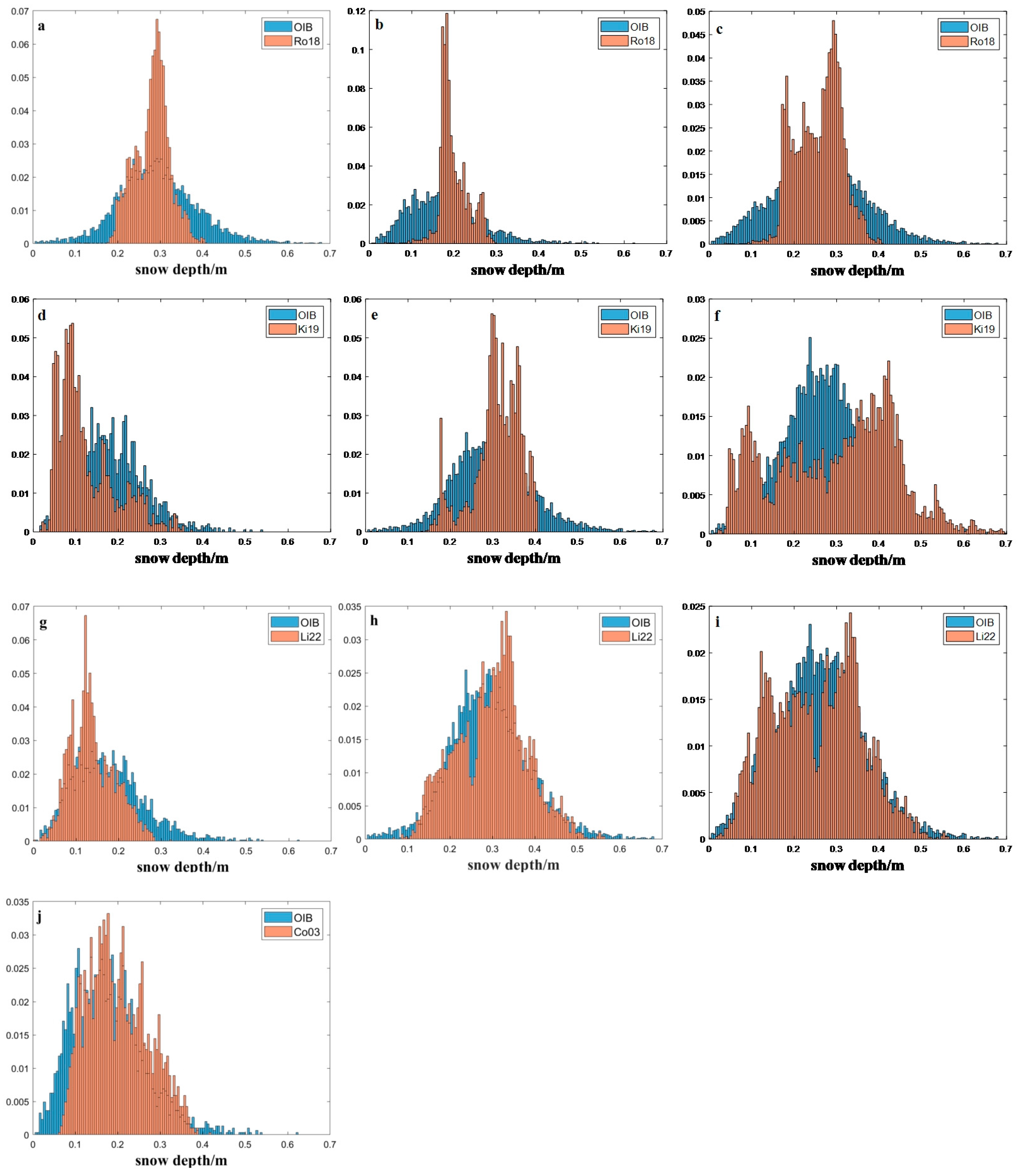
To ensure the feasibility of accuracy evaluation, 1,398,689 points were selected for processing in the 10 months from 2013 to 2019. Based on the accuracy evaluation results (Table 2), the Ro18 algorithm performs better for the entire Arctic as well as different ice types as it is developed from the OIB dataset. In terms of performance, the Ro18 algorithm (RMSE = 0.08 m) was followed by Li22 (RMSE = 0.09 m). The Ki19 algorithm (RMSE = 0.12 m) performed the worst among all the algorithms, possibly because the algorithm failed to consider the influence of the water. The Co03 algorithm (RMSE = 0.08 m) performed well in the FYI region. However, considering the spatial distributions of snow depth, the overall depth range of Ro18 was smaller (0.15–0.35 m), making it nearly impossible to invert the large and small depths. To further investigate the distribution trend of the snow depth ranges of each algorithm, statistical analysis was performed (Figure 4, Ki19 considers SIC = 100% only).

Snow depth was significantly lower than the thickness of sea ice. According to the OIB dataset, excluding extreme weather conditions, the snow depth on the sea ice was mostly between 0 and 0.65 m [18], which is consistent with the blue histogram, and there was a significant difference in the results obtained by different snow depth algorithms with the red shown in Figure 4. From the RMSE, the Ro18 algorithm seems to perform best among all methods; however, from the comparison with the OIB snow depth histogram, the result is inconsistent with the data provided in Table 2. The statistical feature analysis indicated that the performance of the Ro18 algorithm for snow depth in the Arctic was not optimal, with the distribution of the majority of snow depths ranging from 0.1 to 0.4 m. It was difficult to accurately determine the results when the depth was too large or too small. This result is consistent with the results obtained by considering the distribution of snow depth. The Ki19 algorithm exhibited significant overestimation and underestimation. The statistical results for the entire Arctic snow depth demonstrated satisfactory performance of the Li22 algorithm. The snow depth ranged from 0.05 to 0.65 m, and the overall data fitting was good, except for minor overestimation and underestimation. This result is consistent with the results of Li et al. [24]; however, they did not conduct the statistical analysis under different ice types, which was also examined to some extent in this study.

The OIB dataset demonstrated that FYI’s snow depth was shallower than MYI’s. Based on the snow depth results for the entire Arctic, Ro18 could not accurately invert deeper and shallower snow depth under both MYI and FYI regions, whereas Ki19 exhibited significant overestimation under MYI and significant underestimation under FYI. The Li22 and Ki19 algorithms demonstrated similar results, and the overestimation or underestimation was relatively low. Co03 exhibited an overestimation under the FYI region.

Briefly, although several algorithms have been developed using AMSR2, there are still certain differences between the inversion results of different algorithms and the measured data, especially for Ro18 and Ki19. These algorithms exhibit overestimation and underestimation phenomena, which leads to significant differences between the inversion results and the measured data. Therefore, the improvement in these algorithms is critical.

For the analysis of results based on Table 2 and Figure 4, the Li22 and Co03 algorithms were used for the final snow depth inversion. As Co03 did not apply to the MYI region, the Li22 algorithm can be used as the standard algorithm applicable to this region (Equation (11)), and the combination of the two algorithms can be used as the standard algorithm for the FYI region (Equation (15)). In order to ensure smoothness at the junction of different ice types, the method of Rostosky et al. was used in this paper for the fuzzy region, and the mean value of snow on FYI and MYI was used to make the transition (in this paper, the algorithm is referred to as MY).

$$\begin{array}{l}{H}_{s\_FYI}=a\times \left(11.01-352.17\times \frac{t_{bice}\left(37 \mathrm{H}\right)-t_{bice}\left(7 \mathrm{H}\right)}{t_{bice}\left(37 \mathrm{H}\right)+t_{bice}\left(7 \mathrm{H}\right)}\right)\\ \hspace{1em}\hspace{1em}\hspace{1em}\hspace{1em}\hspace{1em}\hspace{1em}+\left(1-a\right)\times \left(2.9-782\times \frac{t_{bice}\left(37 \mathrm{V}\right)-t_{bice}\left(19 \mathrm{V}\right)}{t_{bice}\left(37 \mathrm{V}\right)+t_{bice}\left(19 \mathrm{V}\right)}\right)\end{array}$$

(15)

where $a$ is the value of fusion weight.

The least squares method was used in this study to determine the value of fusion weights. The six years of OIB-measured data from 2013 to 2018 were used as the benchmark, and the AMSR2 inversion results were fitted to minimize the dataset-related errors. The results indicated that the Co03 algorithm had a relatively high weight (a < 0.5), which is consistent with its optimal performance (Table 2).

To further determine the feasibility of this algorithm, a correlation analysis was conducted between data derived from the algorithm and the OIB data (

Table 3. Accuracy evaluations of the Co03, Li22, and MY (using AMSR2 TB) using RMSE (m), bias (m), and R based on OIB-measured snow depths (April 2019, 28,855 points) over FYI.

FYI	Co03	Li22	MY
R	0.47	0.40	0.46
RMSE/m	0.10	0.12	0.09
bias/m	0.01	−0.06	0.01

). As Co03 was not applicable to the MYI region, an accuracy evaluation was conducted for the snow depth in the FYI region. Compared with the other two algorithms, MY exhibited a certain degree of improvement in RMSE (0.09 m) and bias (0.01 m), and the improvement was more significant compared to Li22. The correlation coefficient of MY (0.46) was relatively lower compared to that of Co03 (0.47); this could be due to the poor results of Li22. Considering the correlation coefficients of other algorithms, this result was within the acceptable range.

3.3. Snow Depth Inversion Algorithm from the MWRI

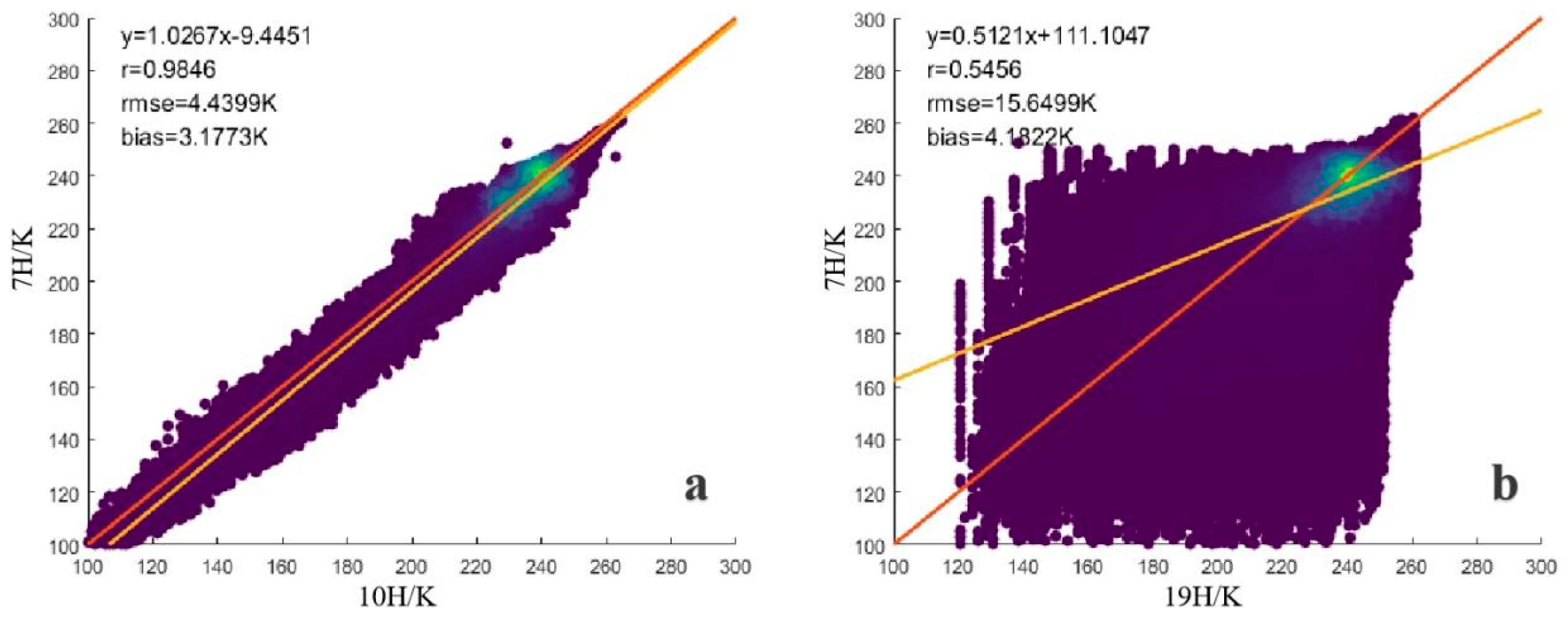
Unlike AMSR2, MWRI does not have the brightness temperature of C-bands. Therefore, the replacement of 7H brightness temperature by other channels has become a key issue in determining the suitability of the algorithm for MWRI. To address this issue, we attempted to use other AMSR2 channels as substitutes. The brightness temperature of 22 GHz and 85 GHz is not available because it is highly sensitive to atmospheric conditions, especially water vapor. Therefore, the correlations between 10 GHz, 19 GHz, and 7 GHz were examined (Figure 5). To minimize the impact of temporal and spatial variability, data from November 2012 to April 2022 obtained from AMSR2 were randomly selected for five days each month to conduct scatter comparisons.

According to the analysis, there is no correlation between the brightness temperature of 19 H and 7 H, and the emission characteristics of 19 H and 7 H are highly random. However, compared with 19 H, the emission characteristics of the Arctic region at 10 H and 7 H are very similar; the correlation coefficient reaches 0.98, the RMSE and Bias are less than 5 K, and the fitting curve almost overlaps with the 1:1 curve. These results are in good agreement with those obtained by Chang et al. based on the MEMLS model (dry snow, radius = 0.5 mm, incidence angle = 50°) [30] and based on the MEMLS model simulated by Li et al. (dry snow, radius = 0.75 mm). As the snow depth changes from 5 to 70 cm, TB (10 H) decreases by about 6 K; in other words, the small error in brightness temperature has little influence on the snow depth retrieval result [18], which makes it possible to use this algorithm for MWRI snow depth inversion, so the 10H post-processing will be directly used to retrieve the snow depth in the subsequent process.

To make the algorithm suitable for MWRI, it is essential to ensure data consistency and standardize the brightness temperature values from different sensors to a common benchmark. In this study, inter-sensor calibration was conducted to align TB measurements from AMSR2 and MWRI. The first step is to find the observations of the same ground object captured by two satellites during the same or similar observation time for calibration. To ensure the accuracy of the results, the strip data and grid data were converted to the polar stereographic projection with a spatial resolution of 25 km. The inter-sensor calibration was conducted for each required channel, using a spatial window of 25 km and a temporal window of 1 day as calibration parameters. Subsequently, linear regression coefficients were computed using matched TB data for each band.

To enhance the accuracy of the calibration coefficients, the data on the 1st, 6th, 11th, 16th, 21st, and 26th days of each month (132 days) was chosen for calculating the calibration coefficients. Using these coefficients, MWRI’s calibrated TBs were then utilized to estimate snow depth. To validate the calibration results, the April 2019 test batches were selected. After calibration, the correlation coefficient for each band is above 0.9.

The MWRI-based snow depth inversion algorithm was generally acceptable after calibration. However, because the SIC provided by the National Satellite Meteorological Center (NSMC) is based on the NT2 algorithm, there is a certain difference between the snow depths obtained using different SICs. Therefore, recalibrating the snow depth products with different SICs is an essential step, and the calibration method was consistent with the brightness temperature dataset calibration. According to the results of the comparison of the products with different SICs by Zhao et al., AMSR2/ASI performs better; therefore, the snow depth acquired based on ASI was used as a benchmark to calibrate it acquired by NT2 [31]. Subsequently, the data were merged to obtain the algorithm for snow depth on Arctic Sea ice suitable for MWRI.

4. Result

4.1. Performance of the New Snow Depth Algorithm and Parallel Comparison

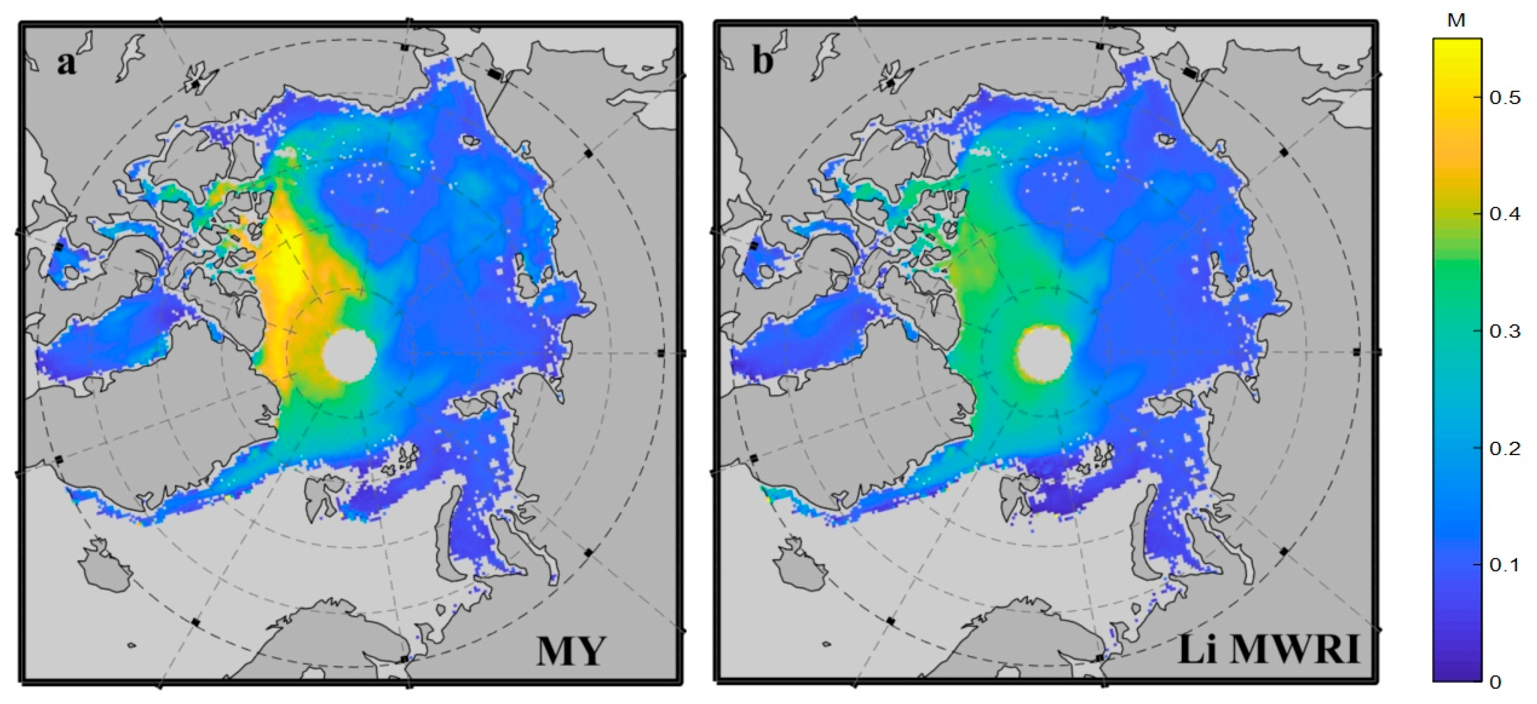
To evaluate the feasibility of the algorithm, it was applied to the brightness temperature dataset of MWRI, and then the snow depth on the Arctic Sea ice was inverted (Figure 6a). Li_MWRI provided the first algorithm of snow depth on the full coverage of the Arctic sea ice from MWRI. A comparison was made between MY and this algorithm to evaluate the correlation. However, because the algorithm is developed and constructed based on FY-3B/MWRI, it is necessary to perform inter-satellite calibration before comparing FY-3D/MWRI and FY-3B/MWRI. In the paper, the overlap period between the two was selected from January to April 2019 (with FY-3B/MWRI data starting and ending from 18 November 2010 to 19 August 2019 and FY-3D/MWRI data starting and ending from 1 January 2019 to present) for calibration, and the snow depth calculation of the algorithm was performed based on the calibrated data. In order to compare their spatial distribution, the monthly average snow depth of Li_MWRI in January 2019 is shown in Figure 6b. It should be noted that in order to measure the monthly average snow depth, all available data for a month were used and averaged. However, this result can only be used for comparison and does not represent the actual average depth, especially during the growing season of sea ice.

Overall, the spatial distribution of the two algorithms was relatively consistent, and the areas with thicker snow depth were mainly concentrated in the north of Greenland and the Canadian archipelago. Most of the area was covered by MYI, while the north of Eurasian had shallower snow. The spatial distribution is consistent with the snow depth products from the University of Bremen (not shown here). However, there was a significant difference in the range of snow depth between these two algorithms. Considering April 2019 as an example, the main depth range obtained by Li_MWRI varied between 0–0.4 m, while the main depth range of the algorithm developed in this study ranged between 0–0.5 m.

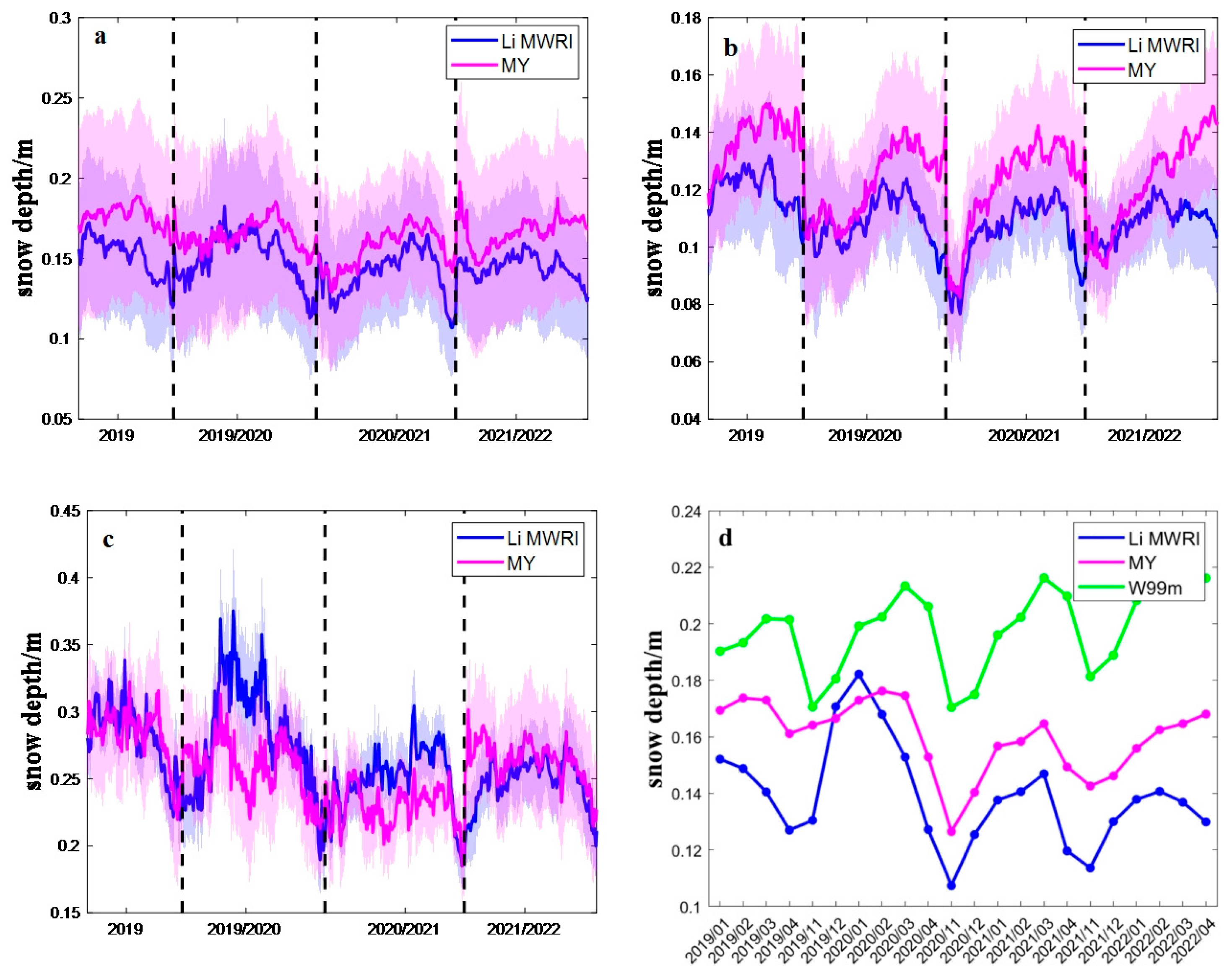
To further evaluate the adaptability of the algorithm in cold seasons, the daily average snow depth from 2019 to 2022 was compared with Li_MWRI (Figure 7a–c) and the monthly average snow depth was compared with W99m (no daily data) and Li_MWRI (Figure 7d). The monthly average snow depth under different ice types is not taken into account here because the product of type is daily products.

In addition to the above-mentioned spatial distribution, the temporal trends of both algorithms were also relatively similar. Overall, from November to April of the following year, data from both algorithms demonstrated a tendency for an initial increase followed by a decrease in snow depths. The maximum snow depth was observed almost every year in March, and the minimum snow depth was observed in November, which is consistent with the results of W99m. Based on the curve results, the snow depth results obtained by the algorithm in this paper and LI_MWRI are consistently smaller than those obtained by the W99m algorithm, and the difference gradually increases over time, aligning with the overestimation suggested by Webster et al. However, on a smaller scale, Li_MWRI did not adhere to this pattern in the spring of 2019 and 2022; the reason remains unclear. On a daily scale, the result obtained by our algorithm was slightly higher than that of Li_MWRI, which may be caused by the snow depth on the FYI being thicker than Li_MWRI.

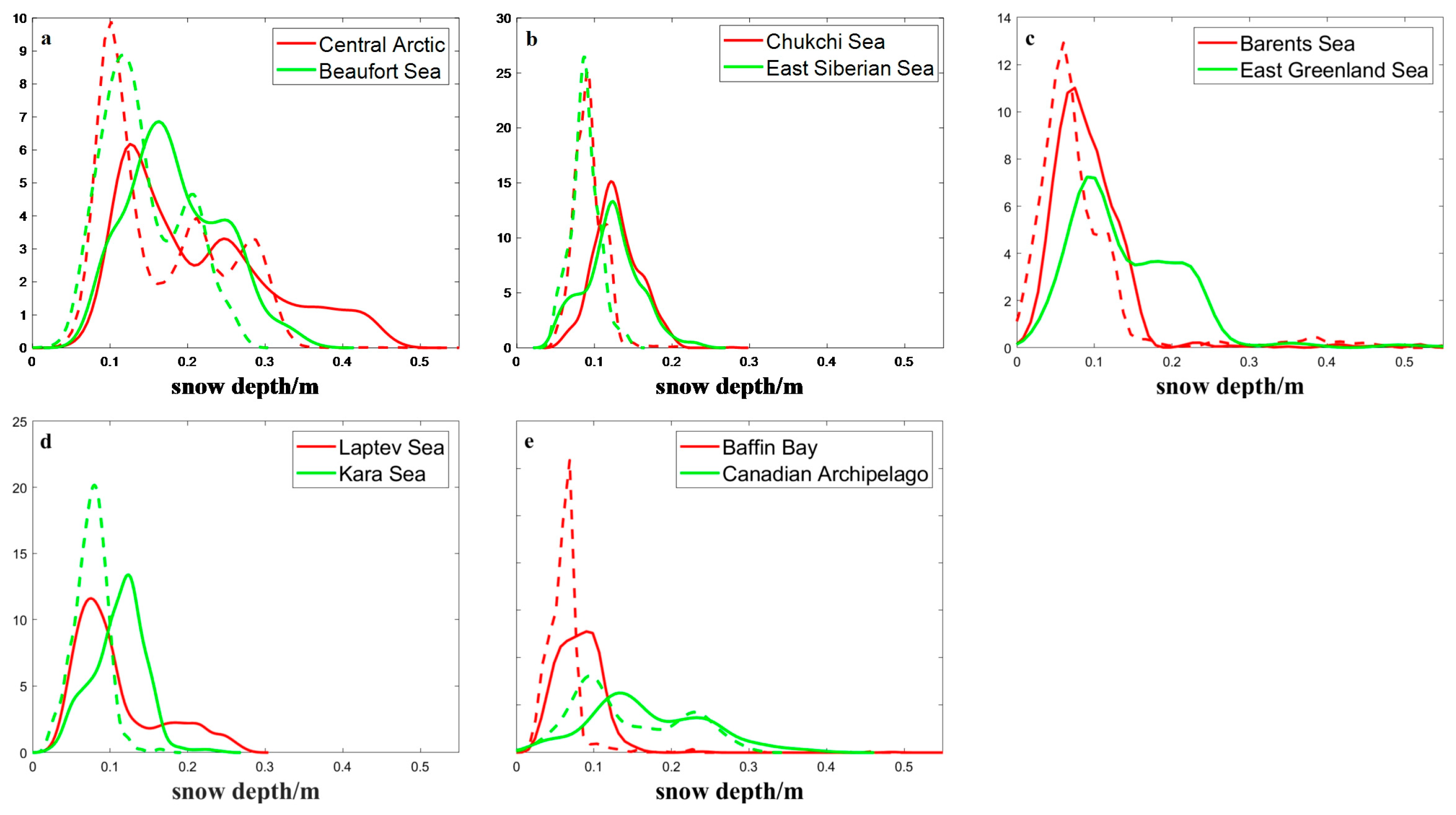
To further evaluate the differences in spatial distribution between the two algorithms, probability density curves were computed for ten sub-regions based on the monthly average snow depth in April 2019 (Figure 8). In addition, the average snow depth in each area was statistically analyzed (

Table 4. Monthly average values (m) of snow depth retrieved by MY and the Li_MWRI algorithm (using MWRI TB) in different sub-regions in April 2019.

Sub-Region	Li_MWRI	MY
Central Arctic	0.17	0.21
Beaufort Sea	0.14	0.18
Chukchi Sea	0.10	0.13
East Siberian Sea	0.09	0.12
Laptev Sea	0.08	0.08
Kara Sea	0.07	0.11
Barents Sea	0.09	0.10
Greenland Sea	0.16	0.16
Baffin Bay	0.06	0.08
Canadian Archipelago	0.14	0.17

).

According to the probability density curve, there is a significant difference in the snow depth distribution between the two in most sea areas: overall, the snow depth values obtained based on the algorithm in this chapter are more extensive compared to Li-MWRI, and their probability values are located in larger intervals, that is, the snow depth obtained by MY algorithm is deeper, the phenomenon demonstrated a decreasing trend from MYI to FYI, particularly in the central Arctic, Beaufort Sea, and Chukchi Sea. The variance between the two outcomes was relatively minor near the Barents Sea and Canadian Archipelago; in the Laptev Sea and Greenland Sea, the probability density curves even overlap, which is also reflected in the mean, especially in areas with larger snow depth (mostly concentrated in the areas where multi-year ice or ambiguous-type ice is located). The numerical values obtained by the MY algorithm are relatively large. The average variation trend of regional snow depth obtained by different algorithms maintains good consistency, with the maximum snow depth in the central sea area and the minimum snow depth in Baffin Bay. However, in the Kara and East Siberian Sea areas, there is a significant difference in the variation trend between the results of MY and the Li-MWRI results. To explore the reasons for this difference, the difference between the two was studied and calculated (not shown here). It was found that the significant differences were mainly concentrated near the New Territories and the Novosibirsk Islands.

4.2. Independent Accuracy Evaluation Using OIB Airborne Measurements

In this section, we conduct an independent evaluation to verify the accuracy of our new product using the OIB-measured airborne snow depth. Because the FY3-D/MWRI brightness temperature is available after January 2019, we selected the OIB measurements in April 2019, which contain 138,244 points for validation. The error statistics are shown in

Table 5. Accuracy evaluations of the Li_MWRI and MY using RMSE (m), bias (m), and R (using MWRI TB) based on OIB-measured snow depths (April 2019) over MYI and FYI.

ALL	MY	Li_MWRI
Corr	0.52	0.42
RMSE/m	0.09	0.10
bias/m	0.01	−0.04
FYI	MY	Li_MWRI
Corr	0.41	0.30
RMSE/m	0.09	0.11
bias/m	−0.01	−0.05
MYI	MY	Li_MWRI
Corr	0.50	0.36
RMSE/m	0.09	0.10
bias/m	0.03	−0.04

, where a comparison with Li-MWRI is also presented.

After experimental data verification in the entire Arctic region, the algorithm in this paper has achieved good improvement compared to the Li-MWRI algorithm, with a 5% decrease in RMSE and a 24% increase in R. Moreover, the results of MY have also improved to a certain extent compared to Li_MWRI on different ice types, and the improvement in snow depth is more significant on FYI (the RMSE of snow depth in FYI region decreased by 2 cm, and the RMSE of snow depth in MYI region decreased by 1 cm). At the same time, in order to ensure that the algorithm has improvements compared to the original algorithm on MWRI, the accuracy of the original algorithm applied on MWRI was also evaluated. As the multi-year ice has not been adjusted, only the snow in FYI was counted here, and the relevant situations under different SIC algorithms were compared: based on NT2 and correction using ASI, the RMSE of the snow depth obtained by Li22 in FYI were 0.11 m and 0.10 m, respectively, the RMSE of Co03 is 0.10 m and 0.09 m, indicating that MY algorithm has improvement compared to the original algorithm and a greater degree of improvement compared to Li22. This conclusion is consistent with the previous section (Table 3). By comparing different SIC algorithms, it can be concluded that the snow depth obtained under correction is slightly better than the NT2 algorithm, further proving that the snow depth obtained based on the ASI algorithm is better.

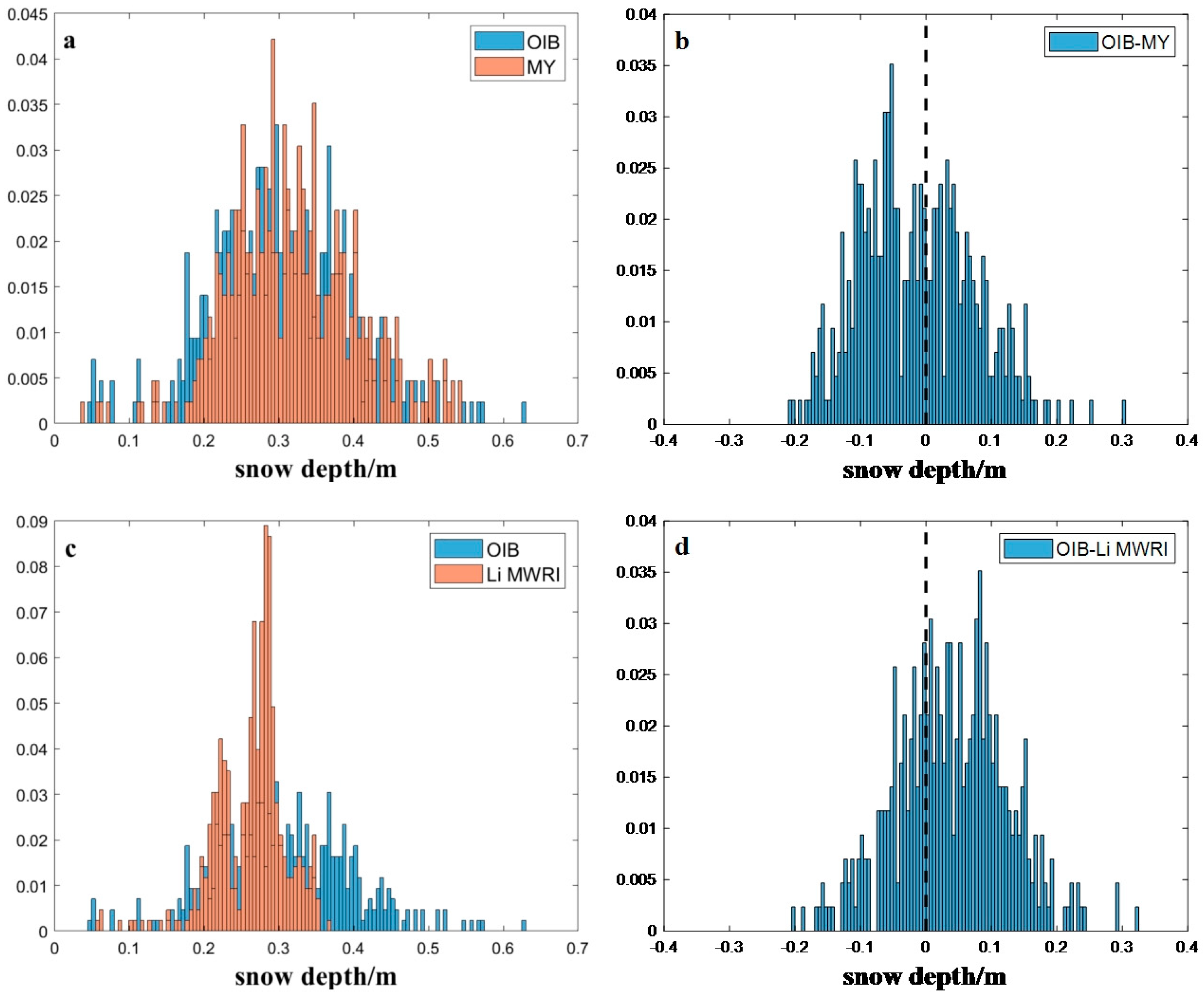
At the same time, to ensure that the algorithm does not suffer from significant overestimation and underestimation, the distribution of numerical values throughout the Arctic was analyzed, and the deviations between derived snow depths and OIB-measured snow depth were estimated (Figure 9).

Similar to the results mentioned in the previous section, the OIB-measured dataset generally ranged from 0 to 0.65 m. This result indirectly indicated that the value of the measured dataset did not consider special terrain, extreme weather, and other special conditions. Except for data at snow depth > 0.55 m, all other depths can be obtained through inversion by MY, and the difference (OIB-MY) at 0 demonstrates a symmetrical phenomenon. The Li_MWRI algorithm exhibited a significant underestimation, and the inversion at the snow depth greater than 0.35 m was not possible. Further, the deviations (OIB-Li_MWRI) also clearly reflected this phenomenon.

5. Discussion

5.1. Influence of SIC on Snow Depth

As one of the crucial factors in snow depth retrieval, the precision of SIC can impact the accuracy of snow depth measurements. In this paper, external products are referenced rather than directly evaluated. The SIC/ASI (the SIC obtained by the ASI algorithm) and SIC/NT2 were used to calculate snow depth. However, the SIC products obtained by the two algorithms also exhibit differences, particularly at the sea ice edge. For instance, on 1 April 2019, the SIC derived from the NT2 algorithm was higher than that obtained by ASI (Figure 2), a finding also supported by Liang’s study [32]. Additionally, a comparative analysis of multiple SIC products by Zhao et al. indicated that AMSR2/ASI data were the preferred product [31]. To minimize data input and ensure the data are primarily from FY-3D and only SIC/NT2 is provided by NCMS, SIC/NT2 is retained, and the data fitting method is employed to reduce errors.

Taking 1 April 2019 as an example, the average snow depth (Co03, Ro18, Ki19, and Li22) of SIC based on the NT2 algorithm is 0.17 m, 0.23 m, 0.22 m, and 0.22 m, respectively. Meanwhile, based on ASI, the snow depth is 0.19 m, 0.24 m, 0.22 m, and 0.23 m. This means that when SIC was involved in the algorithm, the ASI-based snow depth was slightly larger than the NT2-based snow depth, even when different algorithms were used. This phenomenon is more pronounced at the sea ice edge. Zhang et al. also discussed this and found that the snow depths retrieved from the University of Bremen (UB) and NSIDC using the same data source demonstrated that the ASI algorithm-based snow depth was slightly higher than the NT2 algorithm-based snow depth [33]. The RMSE was calculated to assess the performance of various SIC products based on OIB-measured snow depths (

Table 6. Accuracy evaluations of the ASI and NT2 (using AMSR2 TB) using RMSE (m) based on OIB-measured snow depths (April 2019) over MYI and FYI.

ALL	ASI	NT2
Ro18	0.09	0.10
Li22	0.09	0.11
FYI	ASI	NT2
Co03	0.10	0.13
Ro18	0.11	0.12
Li22	0.12	0.13
MYI	ASI	NT2
Ro18	0.09	0.10
Li22	0.11	0.11

). This further supports the conclusion that SIC/ASI performs better.

5.2. Potential Uncertainty of Snow Depth Inversion Algorithm

As an essential aspect of algorithm construction, the accuracy of input data will inevitably influence the accuracy of the obtained results. In order to develop the final snow thickness inversion algorithm, this paper utilized four main data sources, namely OIB, MWRI TB, SIC/NT2, and sea ice type. All of them will lead to uncertainty in snow depth. At present, there is a scarcity of measured data in the Arctic. Data acquisition heavily relies on human subjectivity and accessibility to the environment. Consequently, most of the measured data on snow depth is concentrated in the MYI. At the same time, the spatiotemporal resolution of OIB and MWRI data differs. Although the minimum distance matching method is used to average each point in the grid, there are still some errors, and the verification results are uncertain due to the 5 cm error in the OIB data. In addition, based on the above analysis, the selection of SIC will lead to uncertainty in snow depth. This paper employs different algorithms for MYI and FYI, and misclassification of sea ice type may result in algorithm misuse.

In addition, during the process of constructing algorithms, there are also potential deficiencies. In order to ensure the portability of the snow depth inversion algorithm, this paper compares the correlation between different bands and 7 H and determines the transformation relationship between 10 H and 7 H. However, there are still some discrepancies between them, which will inevitably result in errors in the snow depth inversion. Furthermore, the brightness temperature of open water remains constant in the current snow depth inversion algorithm, which does not reflect the actual situation in the Arctic. Due to its sensitivity, the newly fallen snow cannot be obtained. For the part with SIC < 80%, due to the significant error caused by water, this method is not recommended for use.

6. Conclusions

This study compared four existing algorithms for inverting snow depth, which are applicable for AMSR2 on Arctic Sea ice, and then adapted them to the channels of MWRI, yielding positive results. The enhanced algorithm is based on MWRI and consists primarily of two algorithms (Co03 and Li22). This enhanced algorithm is applicable to the FYI region. The Co03 and Li22 algorithms were combined using a fusion weight and adjusted for the brightness temperatures of 7 H and 10 H, allowing for more precise estimations of snow depth retrievals in the FYI region. In the case of the MYI region, the Li22 algorithm retained the original algorithm. An algorithm for measuring snow depth across the entire Arctic Sea ice was developed after a series of calibrations. This algorithm effectively reduces the overestimation and underestimation of single snow depth inversion models in the FYI region and enhances the accuracy of inversion results using measured data.

The snow depths obtained from this algorithm were compared and evaluated with those from Li_MWRI. It was also compared further with the measured data. The results showed a consistent trend and spatial distribution for both algorithms, with the trend initially increasing and then decreasing between November and April of the following year. Additionally, the snow on MYI was found to be thicker than the snow on FYI. However, there was a significant difference in the range of snow depth between the two algorithms, and MY algorithm’s snow depth was closer to the measured data. The MY algorithm also showed improved accuracy compared to the original algorithm.

However, the algorithm still has a few limitations. For instance, microwave radiation signals are readily absorbed in the presence of liquid water. As a result, this algorithm is only suitable for dry snow. Furthermore, the ASI algorithm (or correction using ASI) was selected as the SIC for snow depth inversion in this study. The performance of other SIC algorithms for snow depth inversion has not been addressed. Further research studies are needed to assess the precision of snow depth measurements obtained using various SIC methods. The differences in algorithms for different types of ice result in variations at the boundaries of ice types, leading to a bimodal histogram. The current algorithm has not resolved this issue, and the use of SIC could be considered for improvement. The algorithm relies on the selection of a sea ice type dataset, so the uncertainty caused by the type needs to be further considered in future processing. Additionally, due to the limited availability of measured datasets at present, obtaining comprehensive data on Arctic snow depth is not currently feasible. Therefore, it is necessary to collect measured data on polar snow depth. Furthermore, with the next-generation FY satellite launch plan in place, 7H can try to adjust the experiment.