Synthetic Data for Sentinel-2 Semantic Segmentation

Abstract

Satellite observations provide critical data for a myriad of applications, but automated information extraction from such vast datasets remains challenging. While artificial intelligence (AI), particularly deep learning methods, offers promising solutions for land cover classification, it often requires massive amounts of accurate, error-free annotations. This paper introduces a novel approach to generate a segmentation task dataset with minimal human intervention, thus significantly reducing annotation time and potential human errors. ‘Samples’ extracted from actual imagery were utilized to construct synthetic composite images, representing 10 segmentation classes. A DeepResUNet was solely trained on this synthesized dataset, eliminating the need for further fine-tuning. Preliminary findings demonstrate impressive generalization abilities on real data across various regions of Quebec. We endeavored to conduct a quantitative assessment without reliance on manually annotated data, and the results appear to be comparable, if not superior, to models trained on genuine datasets.

1. Introduction

Satellite imagery plays a pivotal role in global Earth monitoring due to its comprehensive, objective, and consistent nature. Large-scale phenomena can be captured that might be impossible to observe comprehensively from the ground. Satellite imagery is instrumental in climate change studies. These images can record changes in global temperatures [1,2,3], sea levels, ice cap extents [4], deforestation, and desertification [5]. Post-disaster, satellite images can assess damage and guide recovery efforts [6,7]. In agriculture, satellite imagery helps monitor crop health, irrigation needs, and predict yields, contributing to food security [8,9]. Similarly, in the domain of urban planning, it assists in understanding urban sprawl, managing resources, and planning infrastructure development [10,11]. To make this data actionable, efficient automated processing is needed.

Before the advent of deep learning, various advanced remote sensing methods were employed to analyze satellite imagery. They included spectral indices, unsupervised and supervised classification, and object-based image analysis. Spectral indices, such as the Normalized Difference Vegetation Index (NDVI) and the Soil Adjusted Vegetation Index (SAVI) [12], utilize specific band ratios in multispectral data to highlight certain features, such as vegetation or water bodies. Band ratios can also be used to detect geological features of interest for mining exploration or open-pit surveys [13,14,15,16]. Unsupervised classification methods like K-means or ISODATA (Iterative Self-Organizing Data Analysis Technique) apply clustering algorithms to group pixels with similar spectral properties, requiring minimal human intervention [17,18]. Supervised classification techniques like Maximum Likelihood Classification (MLC) and Support Vector Machines (SVM) involve training a model with pre-labeled samples to classify pixels into specific land cover classes [19]. Object-Based Image Analysis (OBIA) is a technique where the image is segmented into homogenous regions or objects, rather than analyzing individual pixels. Features such as the shape, size, and texture of these objects, as well as their spatial relationships, are used for classification. This approach often yields better results, especially for high-resolution images [20].

These traditional techniques have formed a solid foundation for remote sensing image analysis. However, they typically require manual feature selection and can struggle with complex scenes. Deep learning methods, with their ability to learn features automatically and handle large, diverse datasets, offer a progression in the field of satellite image analysis. Here, semantic segmentation plays a significant role by automating the categorization process of each pixel in an image into distinct classes. Unlike traditional methods, this approach does not just analyze individual pixels but considers their spatial context and interactions, thereby providing a more comprehensive understanding of the image. This allows for high-resolution mapping of diverse features, such as different landforms, bodies of water, vegetation, and urban areas, which can be identified and categorized more accurately [21,22,23]. A key challenge with supervised deep learning techniques is their requirement for substantial volumes of manually annotated data for training. The creation of these training samples is time-consuming and costly, and they are often prone to errors, which may subsequently impair the model’s ability to discern pertinent features within a scene.

Auto-supervised learning methods, including pre-text tasks [24] and contrastive learning [25], offer a partial solution to the challenge of extensive manual data annotation. By leveraging inherent structures and patterns within the data, these techniques can pre-train models without the need for explicit labels. Pre-text tasks, as a category of auto-supervised learning, involve creating artificial tasks where the model must make predictions about some aspect of the input data. This method allows the model to learn useful representations about the underlying structure of the data. For instance, a common pre-text task involves masking some part of the input and asking the model to predict the missing pieces.

Contrastive learning is another form of auto-supervised learning that focuses on learning distinctive features of data by comparing similar and dissimilar examples. The model is trained to identify which data instances are similar and which are not, thus helping to understand the inherent structures within the data. This approach facilitates effective learning of data representations by emphasizing the differences and similarities between data instances. These pre-trained models, whether through pre-text tasks or contrastive learning, can successfully extract higher-level representations from the data and acquire a preliminary understanding of the problem at hand.

However, while auto-supervised learning can establish foundational knowledge, these models cannot perform the required task. A classifier must be trained on labeled data for classification tasks or manually annotated images need to be used for fine-tuning the pre-trained segmentation model. For instance, ref. [25] showed that it could outperform the AlexNet network [26] with 100 times less labeled data on the ImageNet dataset. Also, ref. [27] used contrastive learning for a medical image segmentation task to reduce the need for costly, manually annotated images. In remote sensing, these approaches demonstrated that the need for labeled data could be reduced. Ref. [28] used a combination of contrastive learning and domain transfer to decrease the requirement for extensive data annotation. A semi-supervised contrastive learning method was used by [29] to decrease the need for a large annotated dataset.

Therefore, despite the assistance of auto-supervised pre-training through pre-text tasks and contrastive learning, a significant requirement persists for manually annotated data to fine-tune the model [28,30].

To circumvent the requirement for manual annotation of data, one might explore the availability of pre-existing datasets. Notably, a plethora of datasets designated for segmentation tasks exist, predominantly capturing scenes reflective of daily life from various vantage points [31,32] or they often focus on a vehicle perspective [33]. Within the realm of remote sensing, a substantial number of datasets are likewise accessible. The WHU [34] dataset and the INRIA dataset [35], for instance, encompass tens of thousands of annotated structures for the purpose of building footprint extraction. In the context of land cover analysis, the EuroSAT dataset [36] proves beneficial, albeit it employs patch classification rather than pixel-wise segmentation, a trait shared with the BigEarthNet [37] dataset.

The “Sentinel-2 Water Edges Dataset” is a satellite dataset specifically designed for water edge detection and mapping, leveraging high-resolution images from the European Space Agency’s (ESA) Sentinel-2 mission to monitor changes in water bodies and coastlines [38]. To our knowledge, datasets featuring Sentinel-2 imagery tailored for segmentation tasks are scarce. Although various datasets have been developed utilizing the Segment Anything framework, they, unfortunately, do not accommodate the 10 m spatial resolution nor the pertinent classifications. Furthermore, as delineated in the foundational paper, such datasets are primarily constructed for the objective of pre-training [39].

Consequently, three principal obstacles persist:

-

In practical scenarios, specific classes may be essential for the intended task, yet no dataset comprehensively encompasses these classes.

-

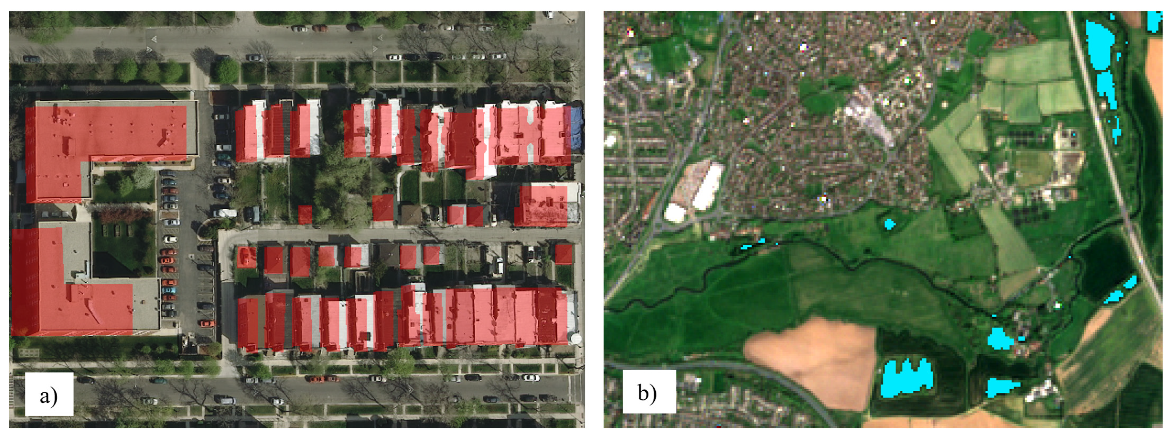
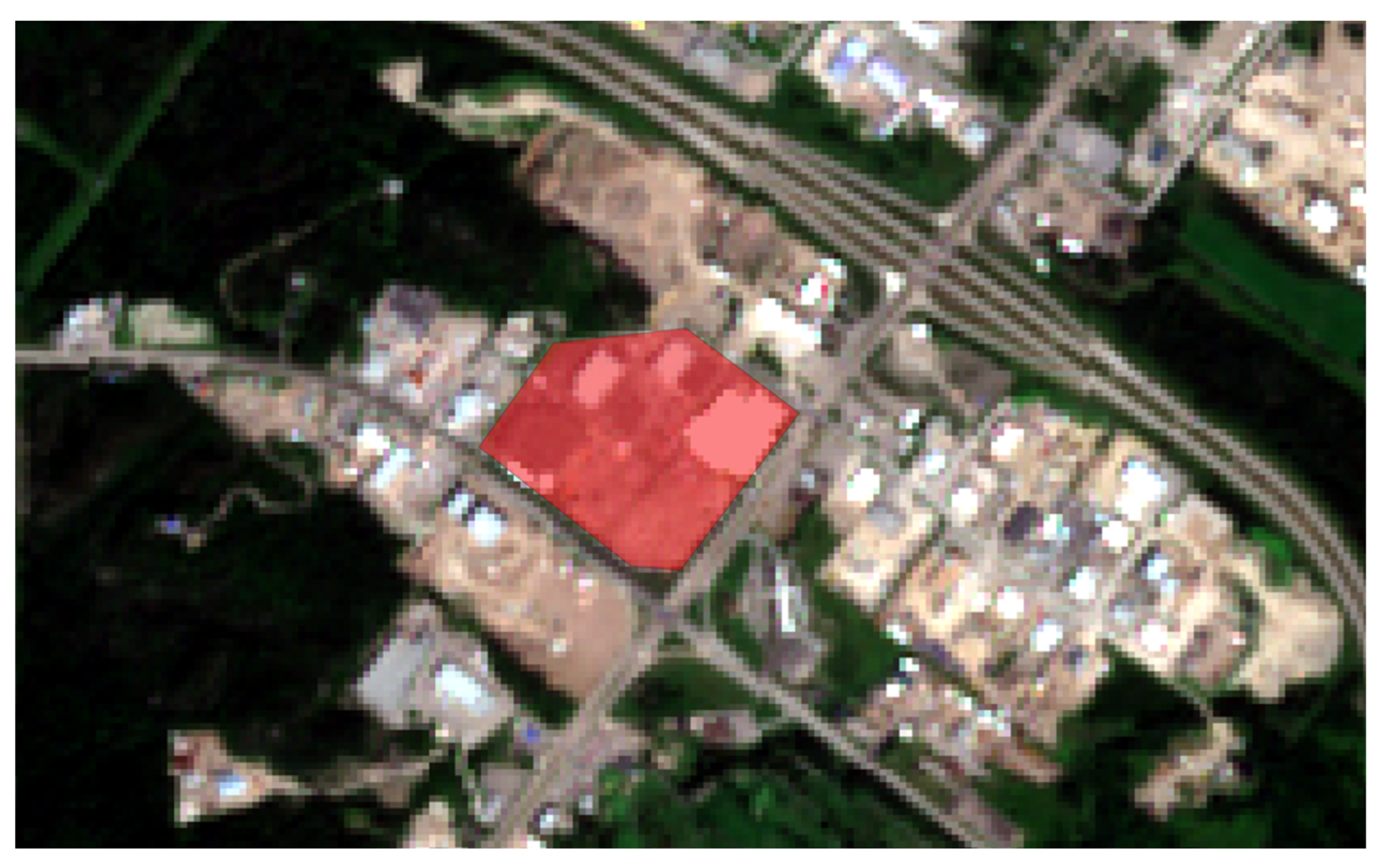
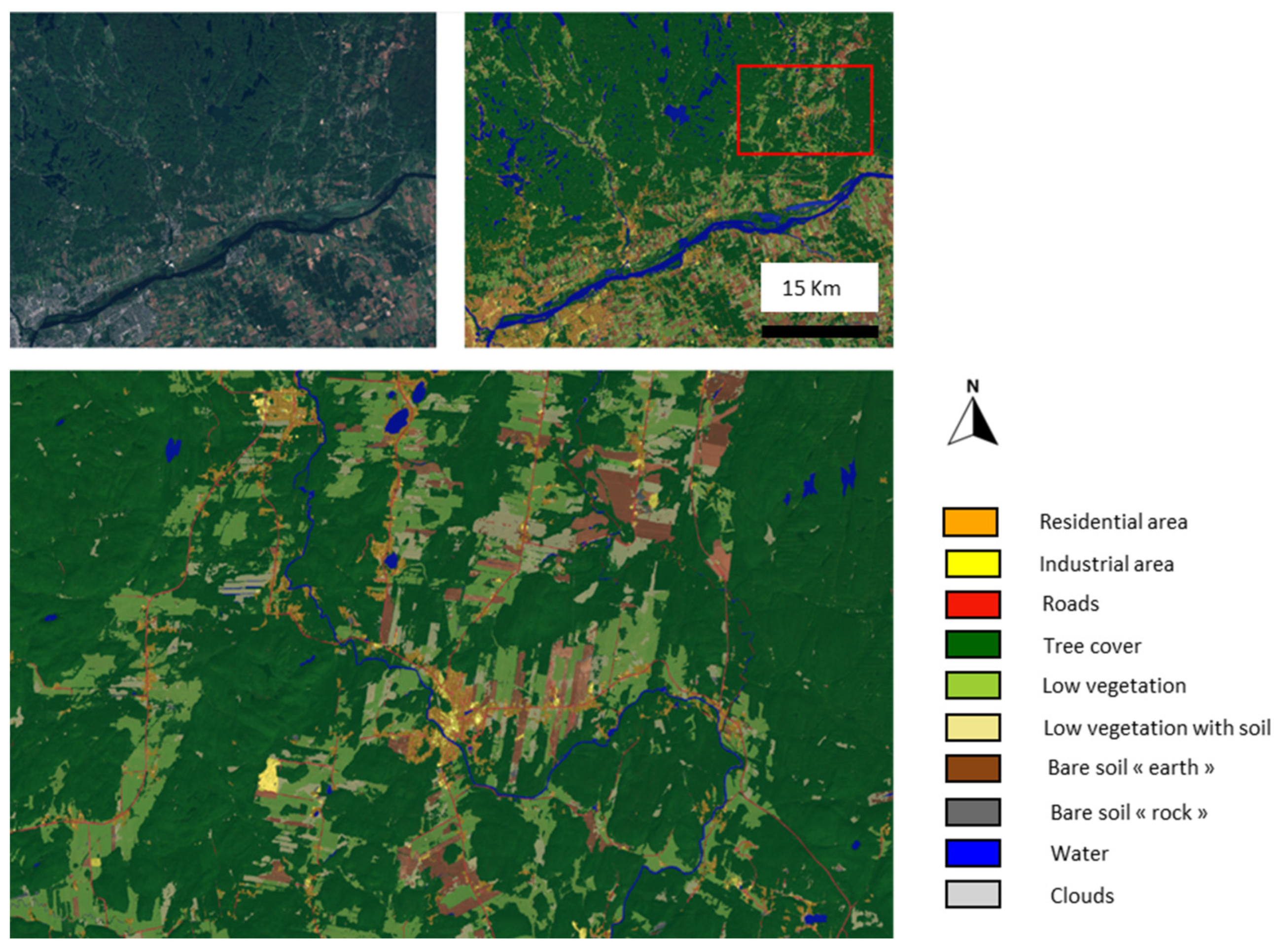
The presence of inaccuracies within these datasets potentially impedes the efficiency of the optimization process throughout the training phase (Figure 1).

-

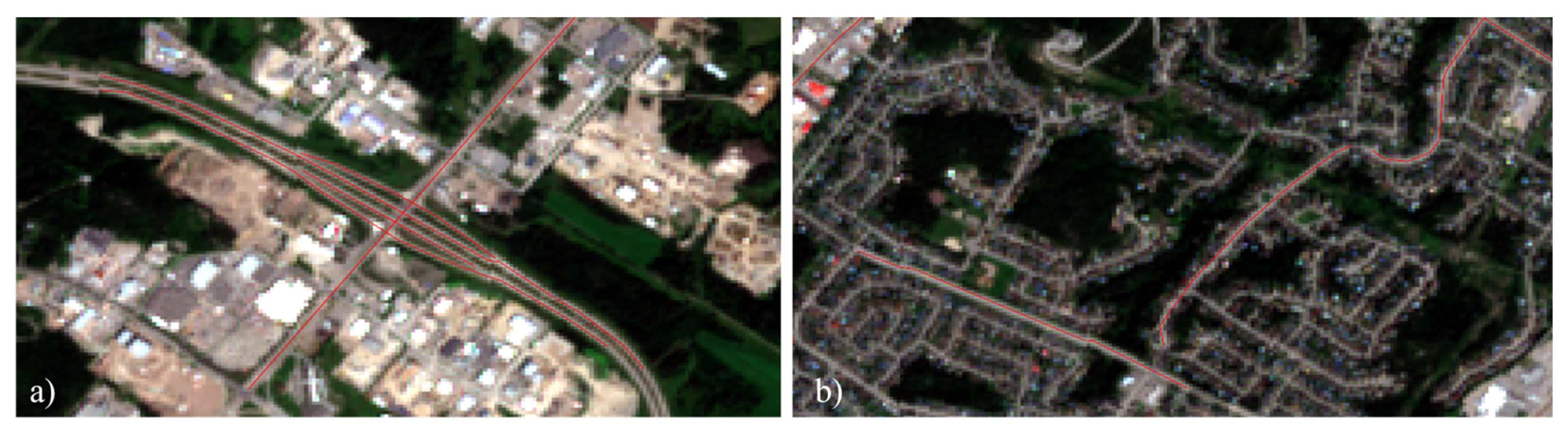
The geographical coverage of these datasets may not align with the target region for segmentation, exemplifying a well-documented issue of generalization.

Therefore, the demand for a bespoke, error-free dataset, accurately reflecting the study area of interest, remains paramount.

Figure 1. There is a discrepancy between the annotation of the buildings and the buildings themselves, likely due to parallax in the INRIA dataset (image “chicago_11”) (a). The water annotation (in turquoise) is missing along the river (SWED dataset image, “24_16”) (b).

Figure 1. There is a discrepancy between the annotation of the buildings and the buildings themselves, likely due to parallax in the INRIA dataset (image “chicago_11”) (a). The water annotation (in turquoise) is missing along the river (SWED dataset image, “24_16”) (b).

Another approach consists of the creation of purely synthetic data. In the domain of autonomous vehicles or drones, simulation is commonly employed to generate copious amounts of error-free data, offering infinite potential variability [40,41,42]. Often, these techniques involve the use of photorealistic Game Engines such as the Unreal Engine. Some synthetic datasets are publicly available but do not concern Sentinel-2 segmentation tasks [42,43,44]. We are not aware of any purely synthetic data used to train models for the segmentation of satellite imagery.

Hence, we present a simpler approach to building a training remote sensing dataset from easy to acquire samples. Despite the simplicity of the simulations, our results demonstrate strong generalization performance on unseen data, effectively reducing the time and cost associated with the manual annotation process. We also compared our results with the ESA’s World Cover [45] and ESRI’s Land Cover [46].

Our main contributions are:

• Introduction of a novel simulation methodology to rapidly create segmentation datasets with minimal human intervention, involving the construction of synthetic scenes from real image samples.
• Training of a model solely on simulated data, which eliminates the need for further fine-tuning on real datasets.
• Demonstration of our model’s impressive generalization capabilities on unseen test data across diverse regions, despite training on limited samples from one area.

Our achievements highlight the potential of simulated training data to reduce the need for extensive manual annotation, while still achieving segmentation quality comparable to that of models trained on manually labeled datasets.

2. Materials and Methods

2.1. Summarized Methodology

To address the need for extensive, error-free training data, we simulated satellite scenes from real samples along with the corresponding semantic maps. Samples were obtained from real Sentinel-2 images available on Google Earth Engine (GEE). We calculated the Intersection over Union (IoU) using pre-segmented polygons and compared our results with two well-known land cover products. We tested various architectures, including DeepLabV3, DeepResUNet, SegFormer, UCTransNet, and Swin-UNet. To enhance the boundary segmentation quality between classes, we utilized a loss weighting map corresponding to class edges. Figure 2 illustrates our general methodology.

2.2. Classes Choice

This study is part of a mapping project for southern Quebec, commissioned by the Ministère des Ressources naturelles et des Forêts du Québec (MRNF). The initial phase of this project seeks to distinguish between natural and artificial terrains. In response to this, we further divided these two primary categories into 10 distinct classes. The natural areas encompass “water”, “forests”, “low vegetation”, “low vegetation–soil mix”, “soil”, “rocky outcrops”, and “clouds”. Conversely, the artificial terrains include “residential areas”, “industrial/commercial areas”, and “roads”. We contend that these 10 classes strike a balanced compromise between classification complexity and utility.

Table 1. Identification cues for the classes and their respective expected confusions.

Classes	Identification	Associated Confusions
Residential Areas	Urbanized areas with a high presence of “single-family” type homes have a particular texture, presenting a mix of buildings and both low and high vegetation.	The strong presence of vegetation might cause confusion with vegetation intermittently interspersed with bare soil. The road network within these zones is very hard to distinguish.
Commercial/and or Industrial Areas	These zones feature large-sized buildings with very little vegetation. One often finds large parking areas or storage yards.	These zones are hard to differentiate from very large residential buildings (boundary between ground cover/use). The road network can “disappear” amidst these zones.
Roads	Roads are comparable to bare soil but have a unique linear structure.	They are very hard to discern in urban areas. It will most likely not be possible to differentiate highways/roads/paths/lanes…
Tree Cover	Does not fit the definition of a forest. Here, the dense vegetative cover is segmented, presenting a distinct texture indicating a high density of trees.	Confusion with forests is rare. Mistakes generally arise from misinterpreted shadows.
Low Vegetation	Represents all low and dense vegetation presenting a smooth appearance reminiscent of grass cover.	Generally, few confusions. This class will contain numerous crops (land use).
Low Vegetation with Soil	Represents all low and not so dense vegetation that partially reveals bare soil. Often crops in early growth or vacant lots.	Generally, few confusions. This class will contain numerous crops (land use).
Bare Soil “earth type”	Surface without vegetation, usually brown in color. The texture can be uniform or present a furrowed appearance.	This class will likely group fields before vegetation growth and also recently cleared lands. The distinction is about “land use.”
Bare Soil “rock type”	Consistent bedrock with a smooth appearance, often in a natural context.	There could be numerous confusions with excavations (construction, mines, earthworks…). Distinguishing among rock/crushed stone/asphalt might be problematic.
Permanent Water Bodies	Often a smooth and dark surface, which might have glints.	It is recognized that water can be easily confused with shadows (very low reflectance). Furthermore, “agitated” water (streams, dam outlets) appears white and becomes very hard to identify as water.
Clouds	Large objects with an extremely high reflectance, often with diffuse boundaries.	Generally, very well segmented. “Transparent” clouds, which let the ground be discerned, are hard to map and deceive the model by significantly altering the radiometry.

provides a detailed overview of these classes along with their associated challenges.

2.3. Sample Collection

2.3.1. Google Earth Engine

Google Earth Engine (GEE) is a robust cloud-based platform facilitating large-scale processing and analysis of geospatial data [33]. GEE boasts a comprehensive archive of satellite imagery and geospatial datasets, with historical data spanning several decades. It amalgamates multiple data sources, such as Landsat, Sentinel-2, and MODIS. The platform provides API support for JavaScript and Python, allowing the development of custom data processing algorithms. Notably, GEE is not exclusive to scientists or GIS experts. Educators, journalists, policymakers, and others have harnessed its capabilities for diverse purposes, positioning it as an essential tool in understanding our evolving planet. For this paper, GEE was utilized to download Sentinel-2 data (https://developers.google.com/earth-engine/datasets/catalog/COPERNICUS_S2, accessed on 5 May 2023). All JavaScript codes related to this paper are accessible at https://github.com/ettelephonne/Projet-MRNF-Occupation-des-Sols/tree/main, accessed on 12 May 2023.

2.3.2. The Sentinel Imagery

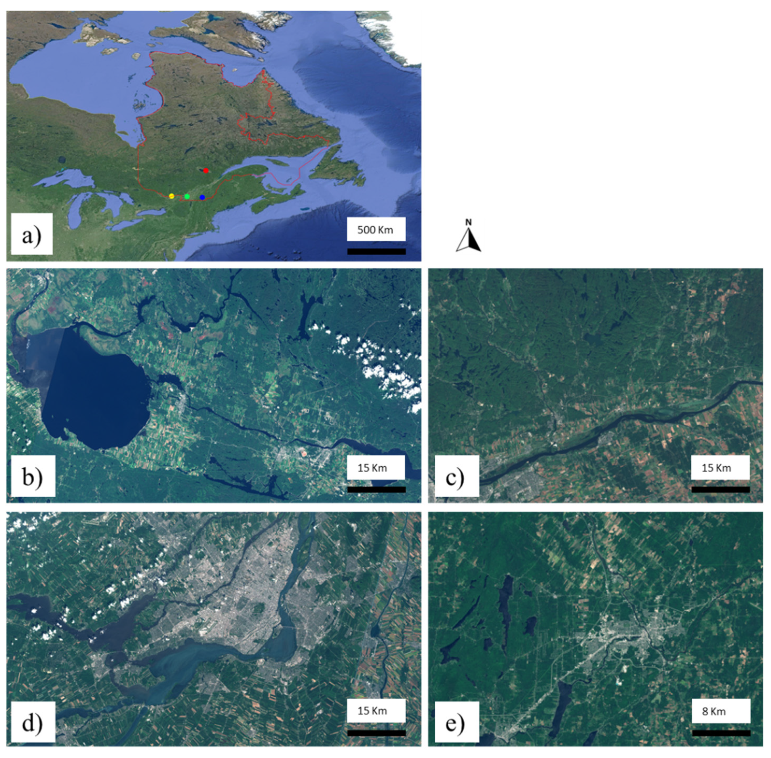
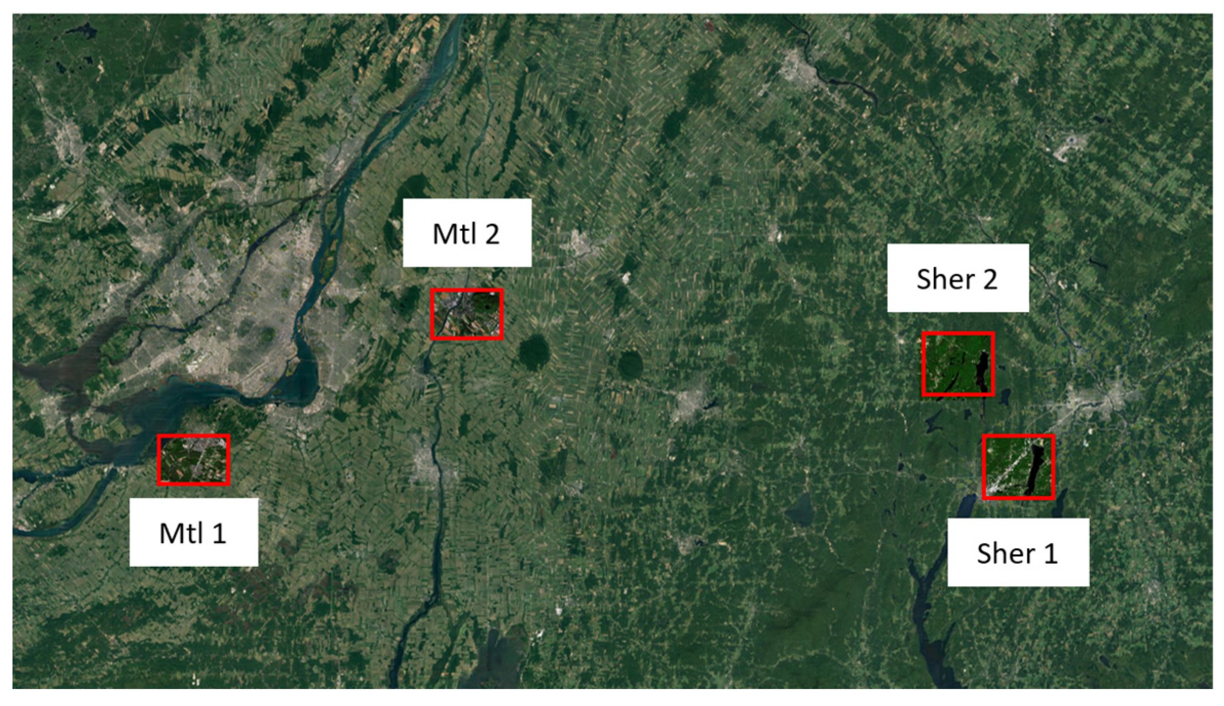
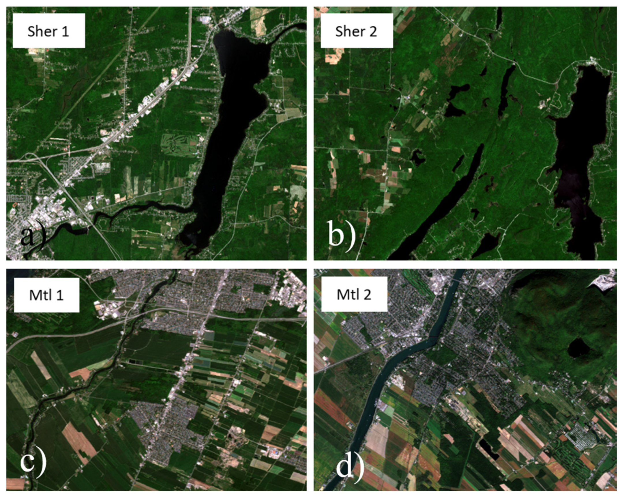
Sentinel-2, a multispectral imaging mission, is a segment of the European Space Agency’s (ESA) expansive Copernicus Program, focused on monitoring Earth’s environment and security. The mission saw the launch of two satellites: Sentinel-2A in 2015 and Sentinel-2B in 2017. Both are equipped with advanced Multispectral Instrument (MSI) sensors that capture high-resolution optical imagery over terrestrial and coastal regions. With its sensors covering 13 spectral bands, Sentinel-2 offers a unique perspective of Earth, producing data pivotal for various environmental and geographical analyses, ranging from monitoring land cover alterations and assessing vegetation health to observing soil and water cover and evaluating the consequences of natural disasters. A hallmark of the Sentinel-2 mission is its rapid revisit and extensive area coverage capabilities, producing global imagery every five days. This feature is invaluable for swift disaster response and tracking rapid environmental shifts. Importantly, the mission’s data are openly accessible, promoting environmental monitoring endeavors worldwide. Within the scope of this study, we exclusively utilized the RGB and NIR bands, both of which offer a spatial resolution of 10 m. This choice aligns with the expectations of the MRNF (Ministère des Ressources Naturelles et des Forêts du Québec) for a land cover map at this specific resolution. Bands featuring lower spatial resolutions, such as those at 20 m and 60 m, were excluded from our analysis.

2.3.3. Study Sites

This research is aligned with a mapping initiative concerning southern Quebec requested by the MRNF. Multiple study sites were selected within this region. Figure 3 showcases the primary areas of interest. These selected regions encompass a range of features corresponding to the classification classes, with each class manifesting in varying proportions. It is important to mention that natural rocky outcrops were notably scarce. To challenge the simulation method delineated in this paper, samples were exclusively collected from the Saguenay region.

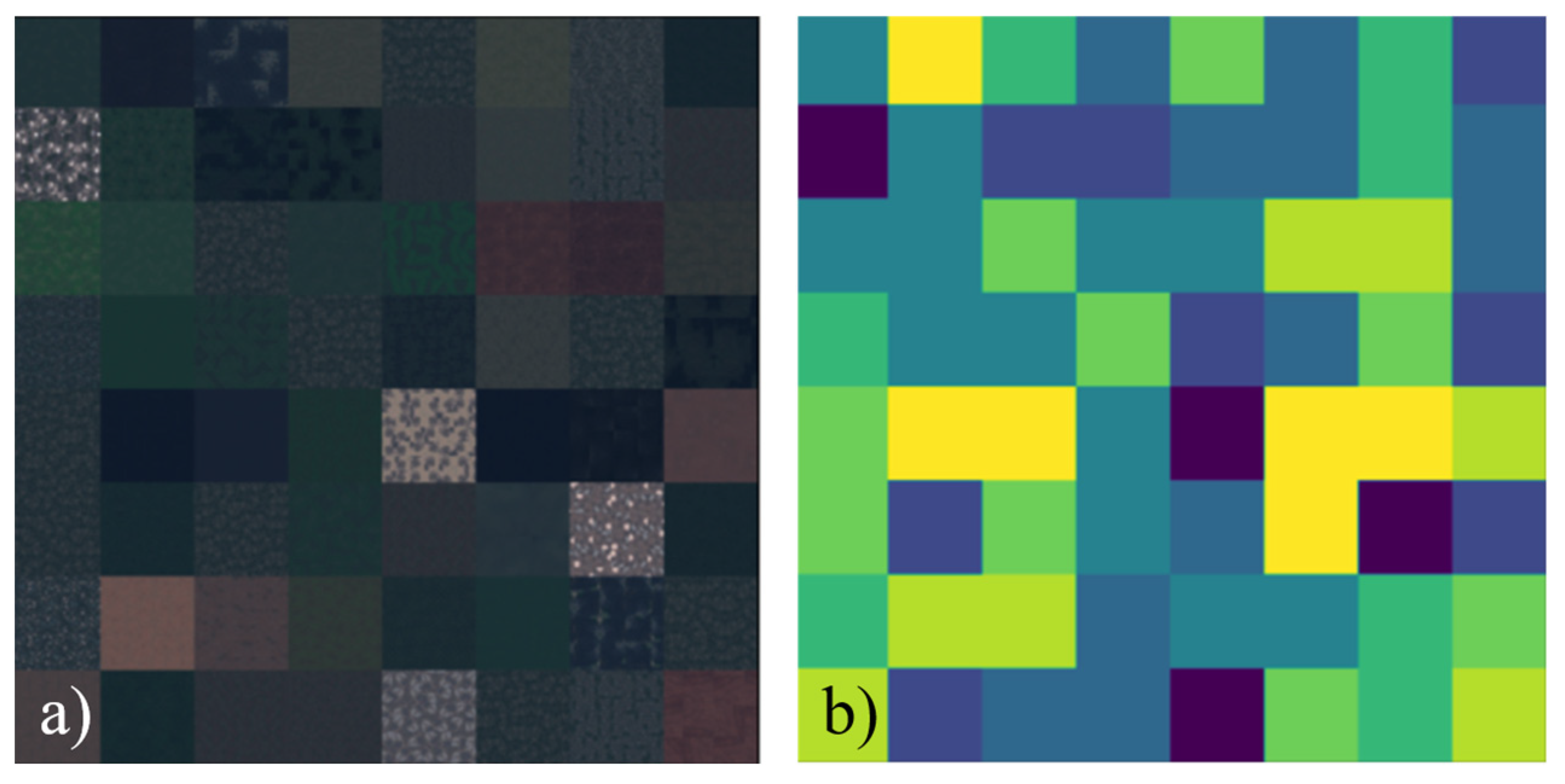
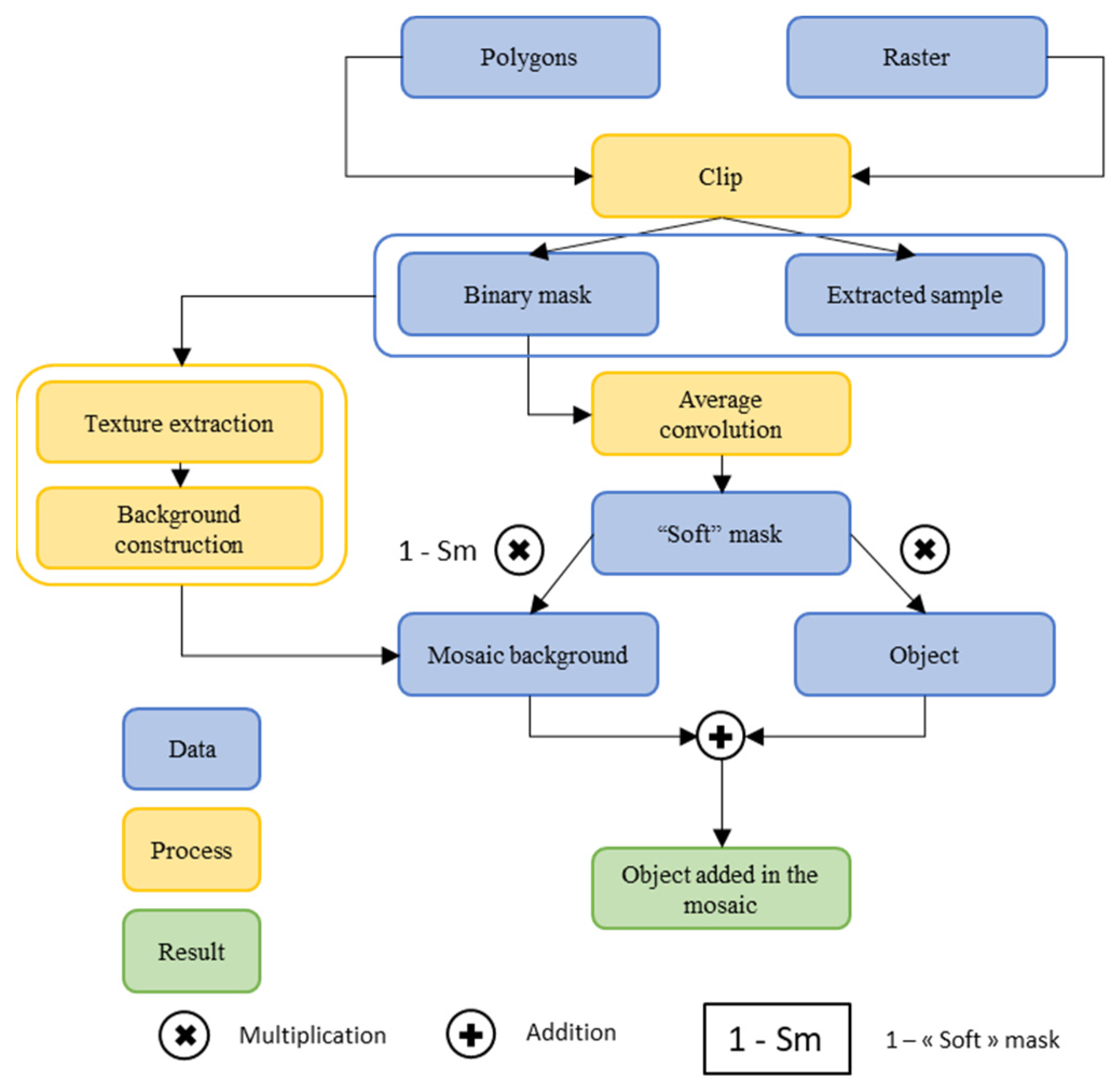
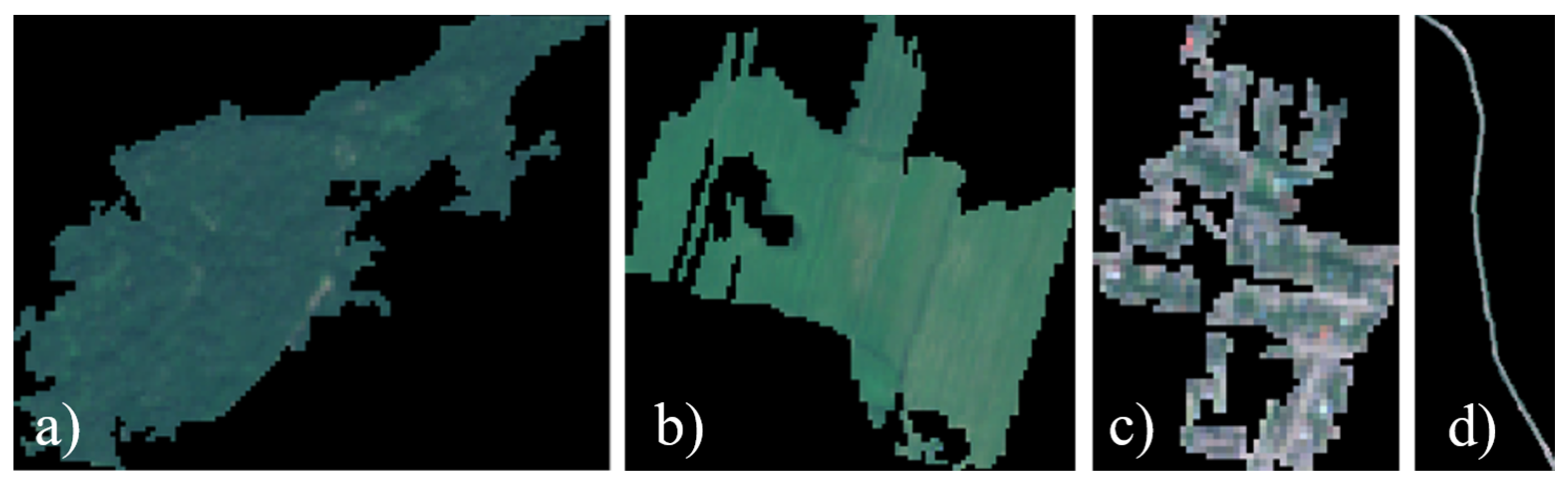
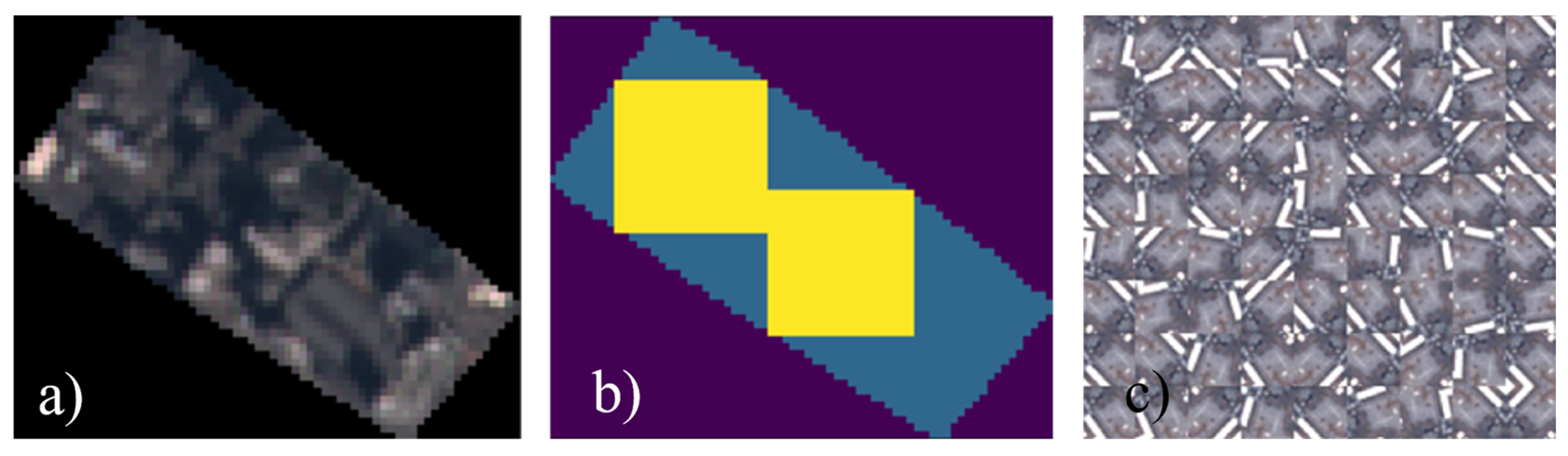
2.4. Scene Simulations

The primary objective of this study was to streamline the labor-intensive process of annotation. Therefore, the sample extraction procedure needed to be efficient and straightforward. We sourced the required data from the Saguenay region. An “object-oriented” segmentation was swiftly executed using the Catalyst (https://catalyst.earth/about/, accessed on 12 June 2023) software, a product of PCI Geomatics, as shown in Figure 4. The selection of this particular software was driven by its availability and the familiarity of our team with its functionality. However, the overarching methodology and the findings of our research do not hinge on the unique capabilities of Catalyst. This initial step facilitated the direct procurement of shapes with realistic and diverse appearances, which is crucial for representing elements such as water, fields, and forests. Opting for polygons simplified the selection process, ensuring the chosen areas were accurate and error-free.

For both residential and industrial categories, there was no need to prioritize precision when delineating boundaries. As demonstrated in Figure 5, which shows a manually selected industrial zone, the accuracy of the boundary lines was not critical. Moreover, consistency in appearance with other elements within the scene was not required. Without a subsequent simulation process, such a basic level of detail in extraction would not suffice for creating a dataset suitable for segmentation tasks. Contrarily, it would have been necessary to annotate all other classes present in the image to ensure the model learns from consistent data, reinforcing the importance of comprehensive data preparation for accurate model training.

Road sampling was derived from a manually created “polyline” vector. The process was straightforward and rapid, as there was no need for meticulous contour management or continuous annotation along the road network, as depicted in Figure 6. Just a 15 m buffer surrounds this vector file, enabling the raster to be intersected with the created polygon.

These polygon-type shape files were then intersected with the images of the Saguenay region to create a sample library (Figure 7). These samples served as the basic material for the creation of simulated data on which the model was trained.

It was interesting to vary the extracted samples to facilitate the generalization of a model to new data. This method is commonly called “data augmentation” in the literature. With this idea of augmentation, textured backgrounds were generated from the samples. As described later, this allowed for the creation of mosaics more quickly. A Python script selected squares within the samples to extract basic textures. These textures then underwent vertical and/or horizontal flips, as well as rotations, and these manipulations were repeated to form a set used later in the simulation (see Figure 8).

Given that the spatial resolution of the RGB-NIR bands of Sentinel-2 is 10 m, it is expected that many objects could be contained within a pixel. Thus, a pixel cannot be considered as “pure” but rather a mixture of its components. The term “mixel” is often used in the scientific literature. Two types of mixtures exist: (1) linear mixing and (2) non-linear mixing. The latter occurs in environments with intertwined materials where a photon interacts with different components. Complex models must be used to simulate the phenomenon of non-linear mixing [47,48]. For linear mixing, also called “surface mixing,” the simulation is much simpler to perform as the mixel is the result of the weighted sum of its different constituents.

The mixing must be performed on pre-existing material. For this purpose, a background mosaic must be created in advance (Figure 9a,b). The mixing for the outlines of the samples that need to be assembled in the simulation is carried out following these steps:

-

Creation of a binary mask that allows for cutting the background.

-

Application of a 3 × 3 “average” type convolution on the binary mask to obtain mixing proportions on the object’s boundaries (Figure 10a), called a “soft” mask hereafter.

-

Cutting the background with softening of the edges (Figure 10b).

-

Softening of the edges for the object to be added (Figure 10c).

-

Sum of the sample and the background mosaic weighted by the filtered mask (Figure 10d).

-

The ground truth is the mask used to “paste” the sample.

The result of these steps is presented in Figure 11 and summarized in the following flowchart (Figure 12). These steps are crucial to ensure that the boundaries between objects closely resemble what one would expect in reality. It is worth noting that manually annotating such a scene would be immensely time-consuming and necessitate multiple correction rounds, yet the outcome might still contain errors.

Figure 9. Illustration of a background (a) with its perfect ground truth mask (b) used to overprint the collected samples. The different colors correspond to different label values.

Figure 9. Illustration of a background (a) with its perfect ground truth mask (b) used to overprint the collected samples. The different colors correspond to different label values.

Figure 10. The binary mask after the average convolution (a). The gradient from yellow to blue corresponds to the mixing ratios. 1 for yellow and 0 for blue. A hole is made in the background (b). Notice the softened border. The exact opposite is applied to the collected sample (c). A softened edge is also added. The result is the incrustation of the collected sample on the background with a linear mixing process on the edge (d).

Figure 10. The binary mask after the average convolution (a). The gradient from yellow to blue corresponds to the mixing ratios. 1 for yellow and 0 for blue. A hole is made in the background (b). Notice the softened border. The exact opposite is applied to the collected sample (c). A softened edge is also added. The result is the incrustation of the collected sample on the background with a linear mixing process on the edge (d).

Figure 11. The simulation result is a patchwork presenting great complexity and variety in the scene (a) with its corresponding ground truth (b). The different colors correspond to different label values.

Figure 11. The simulation result is a patchwork presenting great complexity and variety in the scene (a) with its corresponding ground truth (b). The different colors correspond to different label values.

Figure 12. Flow chart summarizing the simulation process to build a training dataset.

Figure 12. Flow chart summarizing the simulation process to build a training dataset.

In total, 400 images were simulated. This allows for a vast variety of situations since no one is identical to another. All the simulated images were cut into 256 * 256 patches; 85% of them were used as training data and the remaining 15% as validation data. Given that the dataset is entirely simulated, there is no distinction between a validation set and a test set in our context. Additionally, due to the absence of a manually annotated ground truth, we did not utilize any test data in our analysis.

The batch size used, the number of patches the model “sees” before each adjustment of its parameters, was maximized to fit an Nvidia 4080 RTX with 16 GB of memory. Thus, the heavier the architecture, the smaller the batch size. For example, the batch size is 32 for DeepResUNet but 16 for R2-UNet (the larger, the better).

It is important to mention that a “weighted loss map” was calculated for each image/mask pair. Indeed, the original U-Net paper [49] presents interesting improvements by calculating the location of the edges of different classes and adding a weight to these edges. The width of this border is 3 pixels on each side of the class boundary. We chose a weight of three, as higher weights seem not to bring improvement.

3. Results and Discussion

To facilitate a seamless reading experience and avoid excessive toggling between the results and discussion sections, we have opted to intertwine the discussion of results with their presentation. We believe this approach aids in comprehension by allowing readers immediate access to relevant figures as they are discussed.

3.1. Results on Validation Datasets

3.1.1. Architecture Choice

At the beginning of the project, simple simulations made from geometric figures and textures were used. This approach, abandoned later, allowed for an easy comparison of the ability of the DeepLabV3 and DeepResUNet architectures to retain spatial information through the encoding of image features. The first architecture tested was DeepLabV3 with ResNet50 and ResNet101 as “backbones.” As the Figure 13 shows, DeepLabV3 (regardless of its encoder type), is not capable of preserving the image details with sufficient precision. Indeed, semantic segmentation is a compromise between the depth of the architecture, which allows for encoding the maximum amount of information on the broadest possible receptive field, and the conservation of spatial detail. DeepLabV3 can extract information from the image, but the spatial detail is lost. This phenomenon is known in the scientific literature, which is why U-Net type architectures have been developed [50]. The main principle behind a U-Net is to concatenate information from the encoder to the decoder to allow the deconvolution layers to be “guided” by information that would otherwise have been lost.

The SegFormer [51] architecture belongs to the state-of-the-art for segmentation tasks, utilizing both transformers and convolutions. However, our training experiments did not produce results as good as those obtained with DeepResUNet. Here, we assume that (1) even with a pre-trained model, the dataset required by this architecture to achieve good results was too large and (2) numerous parameters can be adjusted within the architecture itself, and this exploration was outside the scope of this work. We have observed the same phenomenon with additional U-Net variants that have also employed transformers, such as UCTransNet [52] and Swin-UNet [53]).

Since DeepResUNet easily achieved the best Intersection over Union (IoU) results on the validation dataset, a challenging metric of segmentation quality, we retained this proven architecture to continue our work.

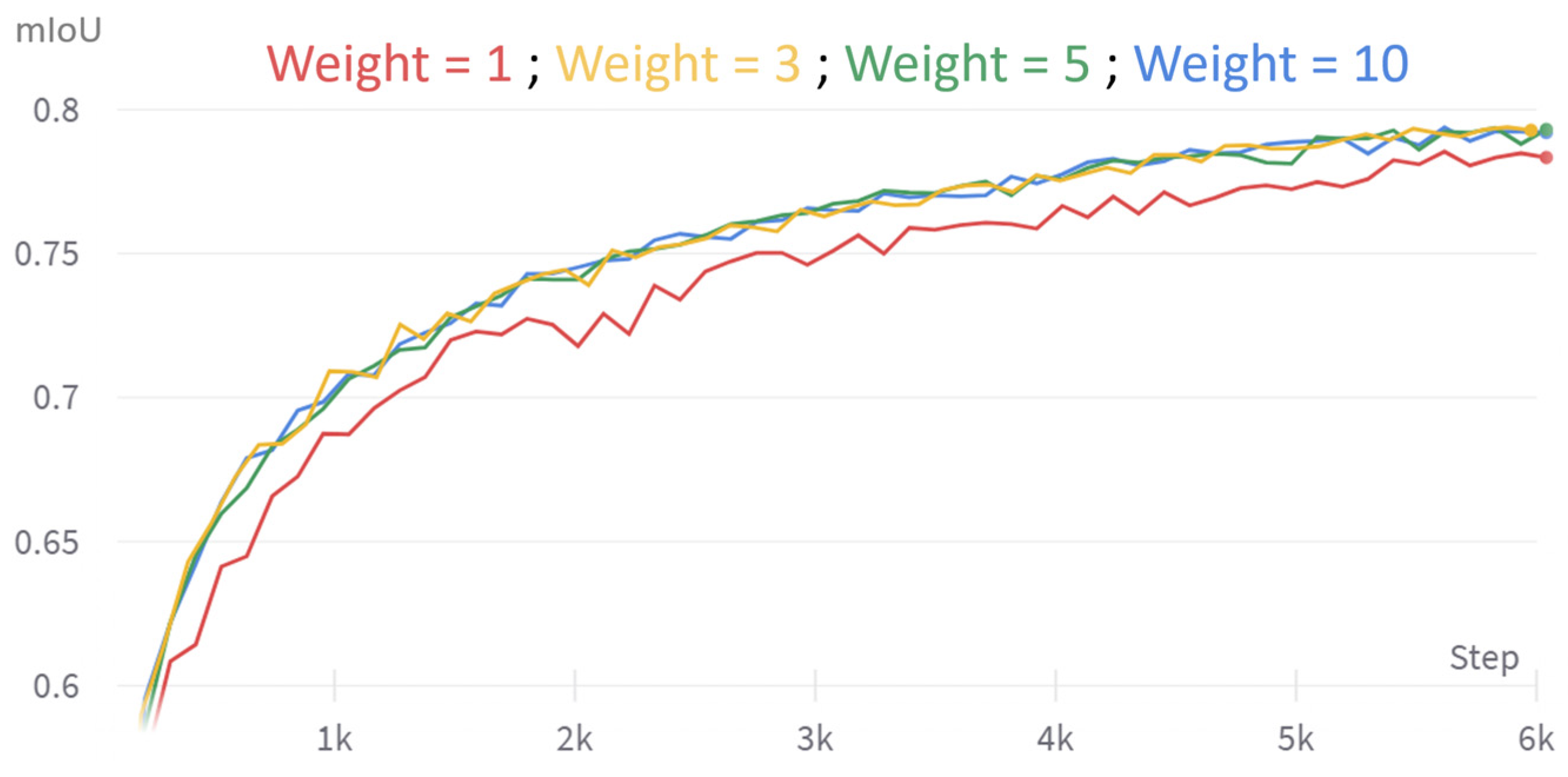
3.1.2. General Training Rules

Validation data are essential in the field of machine learning. Indeed, it is imperative to verify that the rules extracted by the model during the training phase allow it to perform the task correctly on new data it has never encountered. It should be noted that these data were extracted from the same dataset to which the training set belongs. Therefore, validation gives little indication about the model’s ability to generalize to new data but does allow verification that the training is proceeding correctly. For instance, in the case of overfitting, the model will have excellent scores on training data but will fail on validation data. Success on validation data does not, therefore, guarantee good model generalization, but a model that does not work in validation will not work anywhere. The validation patches were extracted from the simulated mosaics up to 15%. The mosaic construction allows multiplying scenarios through repeating basic patterns (the extracted samples). As a result, one may argue that the model has already “seen” the validation data, thereby making this dataset inadequate in representing the learning quality. However, it is important to note that every configuration in the simulated data is distinct. Moreover, here, it is not about proving the performance of a model or learning method on a validation set. This dataset only serves to evaluate various hyperparameter values during the model’s learning while keeping all other factors constant.

We explored how weighting the loss over the edges between classes affected our results. To achieve higher quality segmentations, it is important to focus pixel-level classification at boundaries. In Figure 14, we show an example of inference performed on the edges between industrial areas and other classes. True positives are represented in green, false negatives in orange, and false positives in red.

Hence, we also computed an average IoU based only on the predictions made on the edges. The width of those edges was chosen to be 3 pixels on each side of the boundary. This was conducted to highlight the expected gain of weighting the edges. Indeed, an improvement on these boundaries might not be noticeable in a general averaged IoU simply because the areas in question are too small compared to the total areas.

The curves in Figure 15 displaying the average IoUs on the boundaries highlight a gain of 2 to 3% due to the use of a weight on these same boundaries. It is also observed that increasing the weight beyond 3 has no further impact on the segmentation quality as the results are the same with weights of 5 and 10.

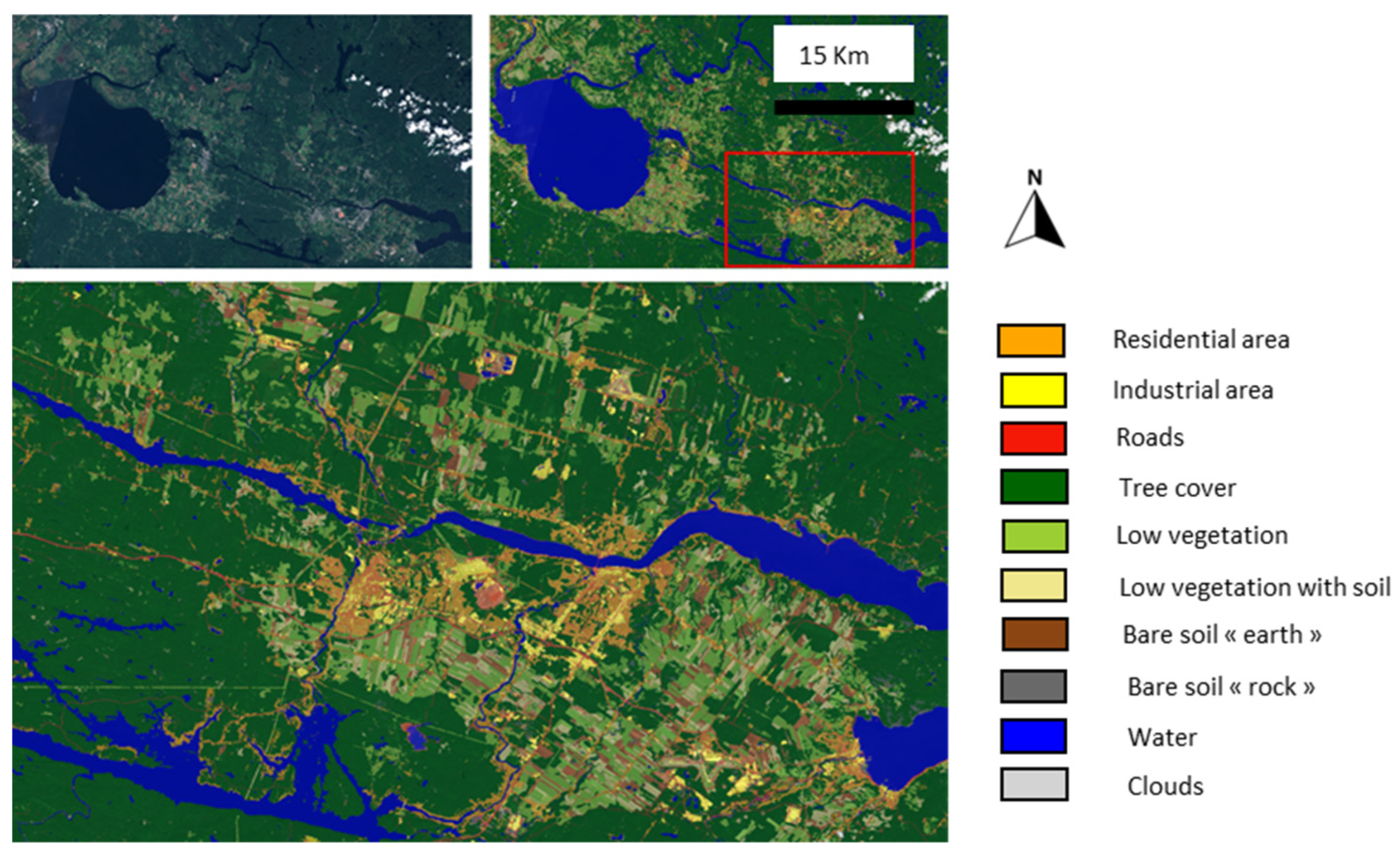
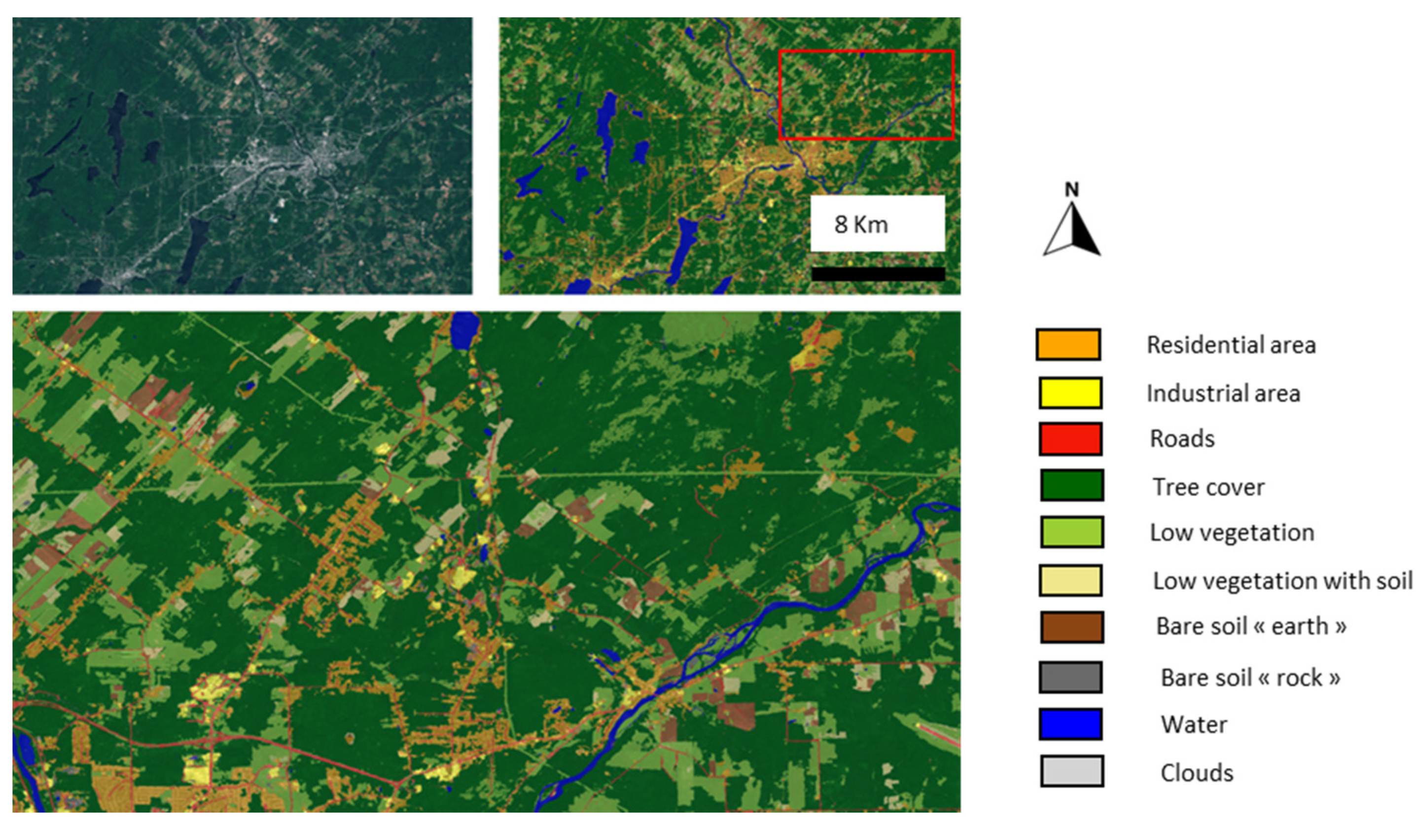
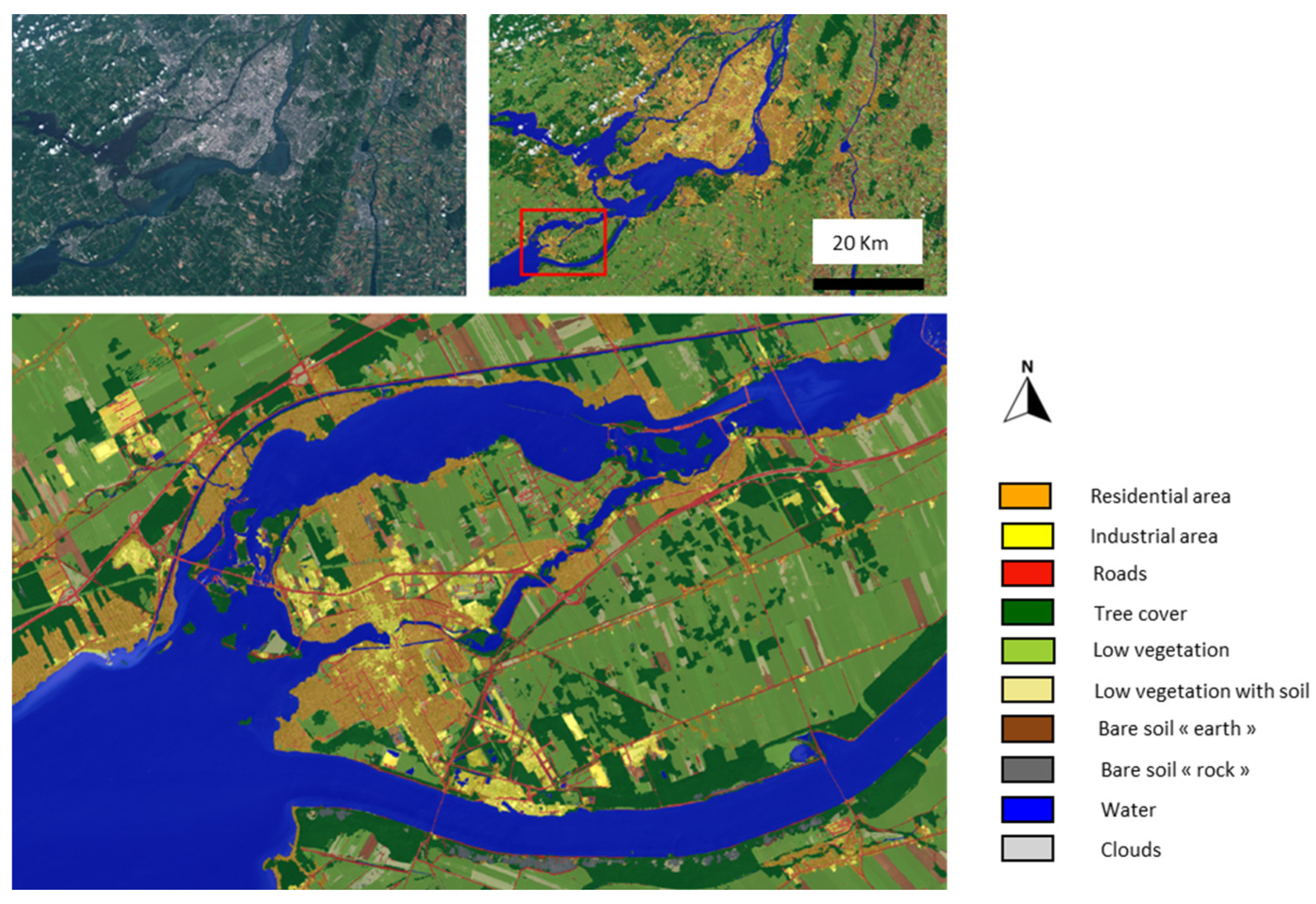
3.2. Results on Test Data

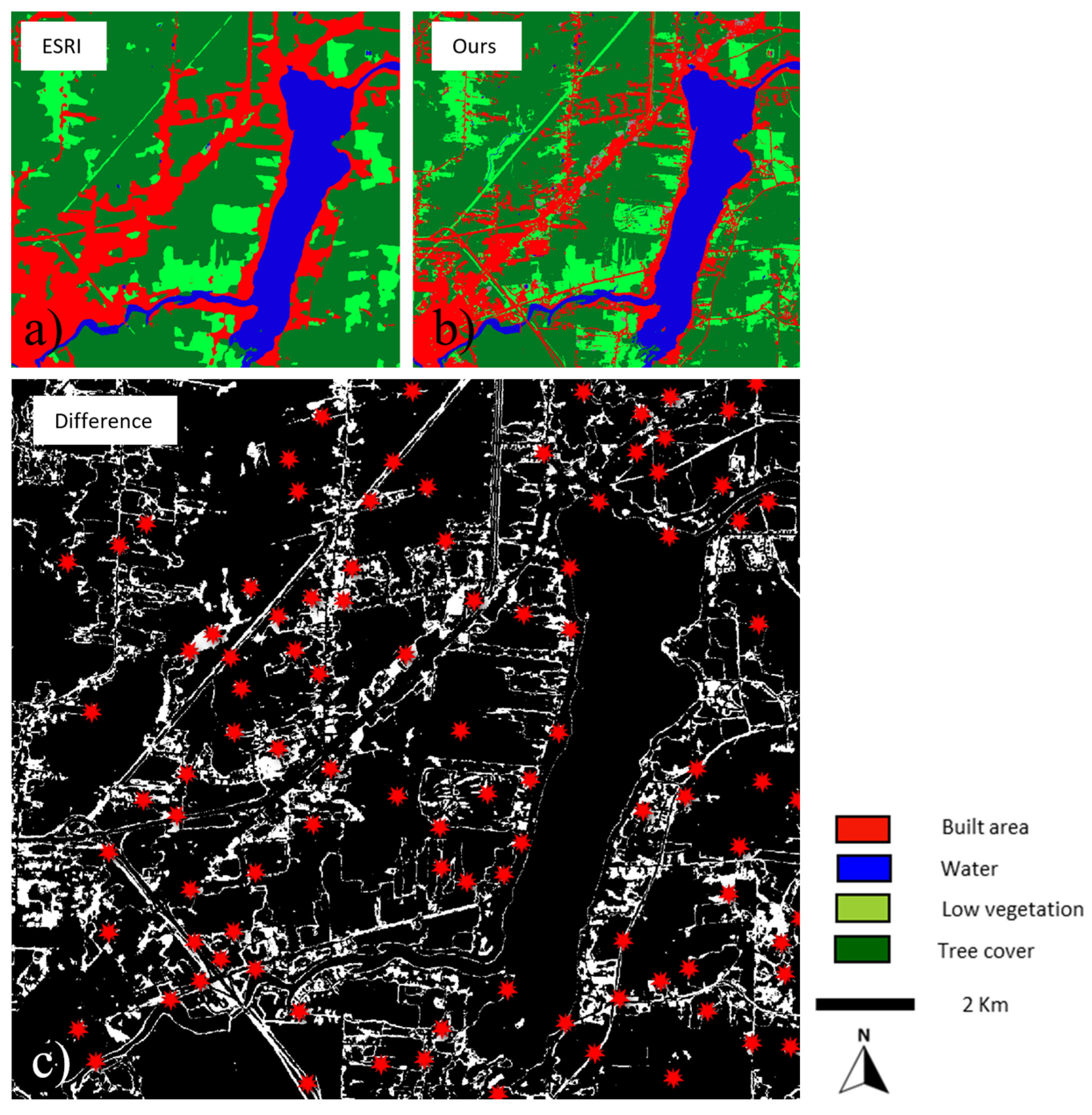
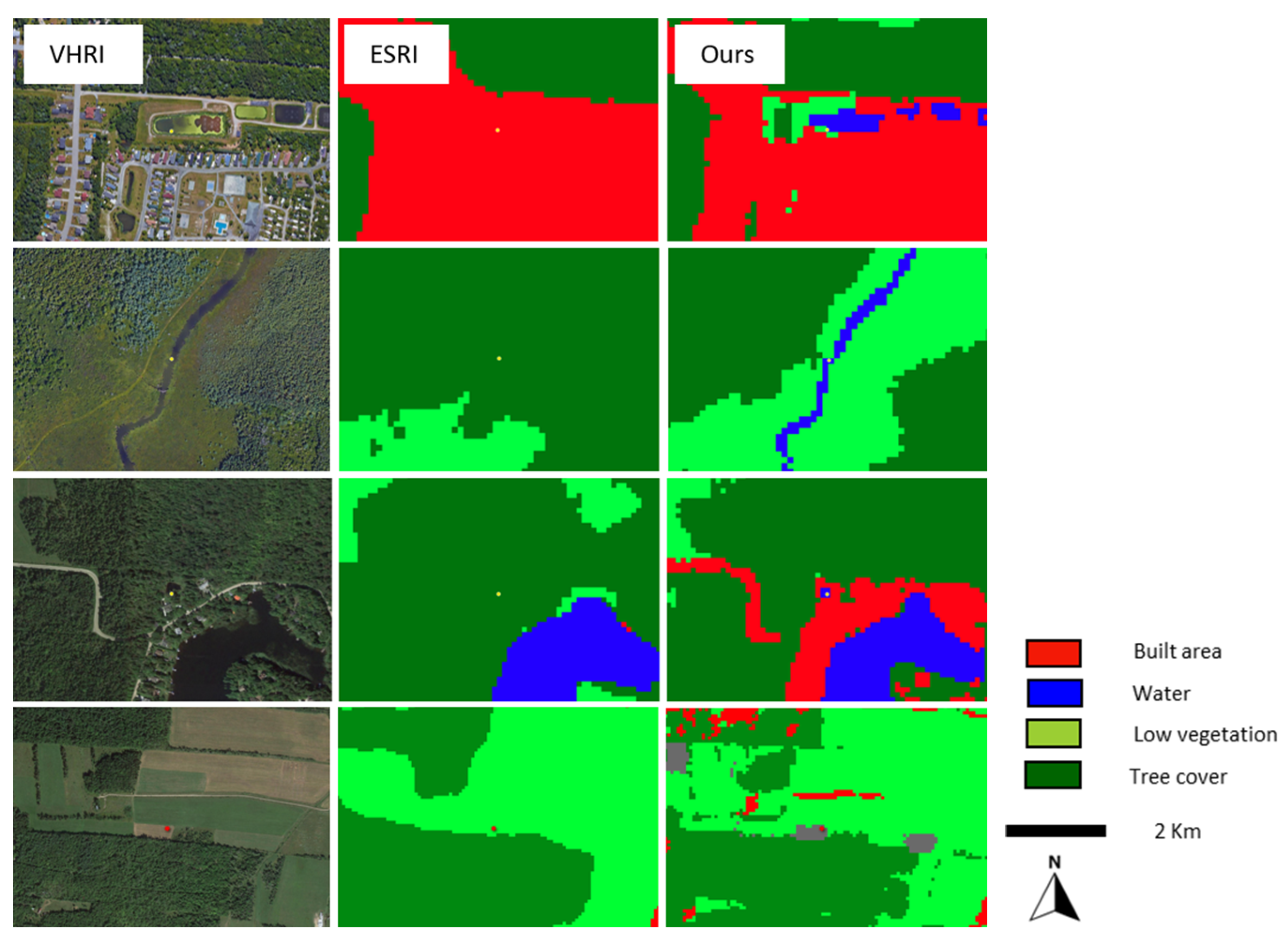
3.2.1. General Overview

After the model was trained on the simulated data, inferences on real images could be made. It is important to note that the model was not adapted or fine-tuned. As a reminder, the data come exclusively from the Saguenay region. The following figures (Figure 16, Figure 17, Figure 18 and Figure 19) aimed to demonstrate the model’s strong ability to generalize from the simulation directly to real data, including regions where no samples were collected.

Qualitatively, the trained model demonstrated impressive generalization capabilities. All segmentation results displayed consistent and coherent patterns (Figure 16, Figure 17, Figure 18 and Figure 19). The consistency of the prediction offers a new perspective on the need to respect the relation between objects. As the simulation loses the correlation between geographical features, a network trained with a synthetic dataset could obviously not learn this prior knowledge. The predictions presented show that this prior knowledge is actually not important. Additionally, the model exhibited robust radiometric performance, seemingly unaffected by atmospheric conditions. This is evident as the model delivered equivalent quality results across geographically distant locations and varied acquisition dates (Figure 20).

However, despite its overall quality, the model exhibited certain errors, especially in regions outside Saguenay (where the samples were collected). These errors can be broadly categorized into three types:

-

Water–Forest Confusion: There was an inconsistent distinction between water and forests. For example, some small lakes were not correctly segmented while others were. This inconsistency lacks an apparent human-observable reason, making it a challenging anomaly to interpret. Different noises on dark waters could be an explanation.

-

Waterways as Roads: Some waterways were mistakenly classified as roads. This could be attributed to radiometric differences, perhaps due to variations in sun elevation and seasonal drying patterns that make some watercourses resemble elongated ground structures.

-

Shadows as Water: Shadows (from clouds, buildings, trees…) in some images were incorrectly classified as water. Given that the elevation in these images is lower compared to the data’s source images, it is plausible that intense shadows could be misinterpreted as water bodies.

It is worth noting that such issues are anticipated during a model’s test phase, even for models trained on manually annotated data. Two key points merit emphasis. (1) The research team was pleasantly surprised by the model’s generalization quality, especially considering the limited sample size used for training. (2) Increasing the spatio-temporal diversity of the samples should address at least partially the aforementioned errors.

3.2.2. General Comparison with Two Other 10 m Products

The simulation method we have introduced stands as a notable advancement in the realm of segmentation. The results are qualitatively good, but an unavoidable question emerges: How does this quality measure up against results obtained using traditional annotation?

This is where our core dilemma lies. The primary drive behind this simulation was to bypass the manual process, known to be costly, lengthy, and challenging. Naturally, for a thorough and holistic evaluation, it would be ideal to juxtapose our test outcomes, generalized across multiple regions, with those of a model trained on conventionally annotated data. Sadly, such a comparison exceeds the scope of this project. Faced with this challenge, we opted to benchmark our results against other segmentations, all also derived from Sentinel-2 satellite imagery. This provides us with a reference point, albeit an indirect one, to gauge the relevance and efficacy of our simulated method. It is crucial to understand, though, that while this comparison offers valuable insights, it does not replace a direct evaluation against manually annotated data. Ultimately, our hope is that future studies might bridge this gap, allowing for a more direct analysis of the efficacy of simulation versus traditional annotation.

The land cover product from the European Space Agency (ESA) discussed in this document was produced in 2020 [36]. It is crucial to emphasize that the land classification performed by our team only used four bands from Sentinel-2 and only from a single acquisition date. The “World Cover” by the ESA required the use of all bands from Sentinel-2 and Sentinel-1 (RADAR imagery), as well as time series of this data and so-called “auxiliary” data, including (but not limited to):

COPDEM: a digital terrain model from the Copernicus project;

OSM: Open Street Map data;

GHSL: Global Human Settlement Layer describing the distribution of human settlements;

GSWE: which provides information about surface water presence.

One can assume that preparing such a dataset was extremely cumbersome and time-consuming. Figure 21 and Figure 22 show views of our results in the region of Montreal. Some classes were merged for fair comparison. We can note the presence of the main road network and the partial presence of the secondary network. Residential urban areas are separated from industrial and/or commercial urban areas. Non-wooded land is divided according to the degree of vegetation: (1) bare, (2) partial cover, and (3) low vegetation cover. These latter classes are grouped under “crops” in ESA’s World Cover. We believe that this rendering is impossible without the use of auxiliary data since it is the use that determines a crop and not its physical cover. We also note that the World Cover provides a poor representation of the degree of urbanization, as the west of Montreal appears to be very underdeveloped due to the significant presence of the “forest” class. Tall vegetation seems to be overrepresented in this classification. However, it is indeed a heavily developed residential area, as our results highlighted.

The ESRI “Living Atlas World Cover” product was obtained through deep learning using a U-Net type architecture [46]. As detailed in the cited paper, the training dataset for this product was manually assembled, encompassing 24,000 Sentinel-2 images, each spanning an area of 25 km². We recognize that the ambitious goal of this project was to classify the entire world, a scope significantly broader than ours. The ESRI team has outlined their annotation methodology: rather than delineating boundaries between classes, they focused on annotating only “pure” classes. Regions in the images that could not be distinctly categorized were labeled as “No Data.” While this approach indeed reduces the time and effort required for dataset preparation, we believe our methodology offers advantages. For instance, the ESRI approach omits the creation of a road network class, which our methodology includes. More critically, by not providing boundaries for training, their dataset lacks the granularity that a boundary-inclusive approach like ours can offer. Moreover, our simulation process has an edge in terms of versatility. It can generate potentially endless variations by randomly arranging the collected samples in the simulated mosaic. This introduces a level of complexity and variability that traditional data annotation might struggle to achieve.

Figure 21 and Figure 22 illustrate the distinctions between our classification and ESRI’s product. For a fair comparison, classes were merged. While ESRI’s overall segmentation appears robust, a discernible “blob” effect can be observed along the peripheries of their predictions. Urbanized areas are slightly overrepresented. Their classification tends to miss smaller roads and only partially captures highways. In contrast, our classification offers greater detail. However, this detailed approach has its challenges: it occasionally misidentifies agricultural paths separating crops as roads.

3.2.3. Quantitative Evaluation

The model discussed in Section 3.2.2 that was used for segmentation was trained exclusively on samples from the Saguenay region, collected in just 3 h. For a more detailed comparison with the ESRI’s Land Cover map, additional samples were gathered from the Sherbrooke and Montreal areas. It is crucial to note that no samples were taken from the test zones depicted in Figure 23 and Figure 24. These four sites are representative of the typical landscapes found in southern Quebec.

Quantitative evaluation metrics, such as Intersection over Union (IoU), precision, recall, etc., inherently demand a ground truth against which predictions can be compared. As mentioned earlier, we did not prepare a ground truth for this study. To address this, we explored two alternative strategies.

The first approach involved leveraging polygons produced by the Object Oriented Analysis (OOA) of Catalyst (https://catalyst.earth/about/, accessed on 12 June 2023). Several polygons were selected for each class across the four test zones, ensuring that no polygon contained multiple classes (Figure 25). This allowed for the computation of IoU values within each polygon. While this methodology offers insights, it comes with certain biases. The selection of polygons was human-guided, not random. This could inadvertently bias the metrics, potentially presenting a rosier picture than is accurate. Larger, more uniform polygons might naturally yield better results, given their inherent simplicity. Conversely, smaller polygons located near class boundaries were frequently disregarded due to high error rates, given they often contained multiple classes. This is particularly true with the classes “industrial/commercial areas” and the “rocky outcrops” where the OOA gives poor results making the comparison difficult (see Figure 25).

Despite these challenges, the IoUs showcased in

Table 2. Mean Intersections over Unions (IoU) for the four test areas. Sher 1: Sherbrooke area 1, Sher 2: Sherbrooke area 2, Mt 1: Montreal area 1, Mtl 2: Montreal area 2.

	Sher 1	Sher 2	Mtl 1	Mtl 2
Forests	0.996	0.998	0.978	0.989
Water	0.999	0.996	0.991	0.983
Low Vegetation	0.950	0.947	0.995	0.967
Low Vegetation/soil	0.928	0.958	0.842	0.879
Soil	0.962	0.965	0.928	0.906
Rocky outcrop	N/A	N/A	N/A	0.020
Roads	0.972	0.924	0.980	0.967
Residential Areas	0.897	0.815	0.926	0.946
Industrial Areas	0.661	N/A	0.756	0.737
Clouds	N/A	N/A	N/A	N/A

can be seen as a reasonably accurate representation of the results. We have made the results accessible (https://ee-dga-couverture.projects.earthengine.app/view/dga-projet-couverture, accessed on 14 September 2023), inviting readers to review and evaluate the segmentation quality themselves.

Following the computation of the IoUs, we sought a quantitative means of contrasting our segmentation against the ESRI’s “Living Atlas” product. We chose the ESRI’s classification for comparison over ESA’s due to its closer alignment with our deep learning segmentation task. It is imperative to underscore that while ESRI’s “Living Atlas” offers global coverage, our focus remains more localized in the south of Quebec. Our primary aim is not to match their extensive scale but to validate the efficacy of our simulation method.

To facilitate a balanced comparison, we merged several classification classes. For instance, our classification comprises three distinct categories (small urban, large urban, and roads), which together equate to the ESRI’s “built area.” Likewise, we combined their “crops” and “range lands” classifications, aligning them with our combined “low vegetation,” “low vegetation/soil,” and “soil” classes. With these merged categories, we then calculated the discrepancies between our predictions and the ESRI output (Figure 26 and Figure 27). Every pixel with a non-zero value indicates a difference in our respective predictions. This disagreement area represents 11.8% of the total. We randomly selected 100 points within these discrepancy zones. For each point, an attribute table column was populated to denote if (1) ESRI’s prediction was accurate, (2) ours was accurate, or (3) neither prediction was accurate (or if the accuracy was ambiguous based on the visual inspection of very high-resolution imagery on Google Earth). In every evaluated zone, our predictions more consistently aligned with the ground truth than ESRI’s. Interested readers can further explore these results at the following address: [https://ee-dga-couverture.projects.earthengine.app/view/dga-projet-couverture, accessed on 14 September 2023].

Upon a more detailed inspection, we suspect that ESRI’s Land Cover might have undergone a post-processing phase, perhaps involving dilation/erosion operations. Their predictions, while often accurate, appear to lack spatial precision. Additionally, no isolated pixels were detected (e.g., a lone water pixel amidst a forest), and the boundary shapes were coarser. Yet, we found no mention of such post-processing in [46], so our observations are speculative. Therefore, this comparative assessment should be approached with caution; ESRI’s global map may not be a direct output from a deep learning model either.

Table 3. Counts of correct classification predictions during visual validation.

	ESRI	Ours	Undetermined
Sherbrooke 1	14	68	18
Sherbrooke 2	12	72	16
Montreal 1	29	58	13
Montreal 2	37	47	16

below encapsulates our comparative findings. It is noteworthy that the Sherbrooke regions consistently outperformed the Montreal areas, a trend also observed in our pre-segmented polygon approach. This led us to note that the Sherbrooke regions had slightly more sample data.

To succinctly encapsulate our endeavors in evaluating the accuracy of our classification without ground truth, it is evident that our product often stands toe-to-toe with, and at times surpasses, other products. While we acknowledge the limitations of our classification not being a global cover, and recognize inherent biases in our quantifications, we emphasize two points to our readers:

-

Our results are accessible online for those who wish to delve deeper.

-

The primary objective of this paper is not to advocate the superiority of our classification, but rather to underline the efficacy and potential of our simulation approach in producing high-quality semantic segmentation.

4. Conclusions

In this study, we have showcased a potential path toward circumventing the tedious and costly manual annotation process to generate error-free remote sensing training sets. Given the persistent demand for expansive training data for model refinement, simulation of such data emerges as an appealing alternative.

Our experimentations were based on Sentinel-2 imagery sourced from Google Earth Engine. By harnessing samples from pre-segmented regions characterized by “pure” classes devoid of inter-class boundaries, we not only expedited the process but also minimized the risk of annotation errors. This research required a mere three hours of sampling to develop a training dataset devoid of errors. The synthesized dataset was constructed by mosaicking the garnered samples, with class boundaries simulated using basic linear mixing—a predominant form of mixing at 10 m spatial resolution. Subsequently, a DeepResUNet model was trained from scratch using conventional methodologies, without resorting to fine-tuning or transfer learning. This model then facilitated a 10-class segmentation spanning extensive territories of Southern Quebec.

To evaluate the quality of our map, we employed a multifaceted approach. We began by computing the Intersection over Union (IoU) metrics, comparing polygons representative of “pure” classes to the predictions from our model. The IoUs spanned between 90% and 100% for widespread classes such as forests and water. Nonetheless, two lesser-represented classes showcased weaker IoU values. Subsequently, we turned to esteemed benchmarks in the field: the ESA and ESRI World Covers. What stood out was that our segmentation, informed entirely by simulated mosaics, consistently matched or even surpassed these gold standards. It is vital to underscore that these benchmarks were derived from models trained on real, manually annotated data. Even so, based on our comparative results, we remain confident that classifications from models trained on such meticulously annotated real data might not have necessarily produced superior outcomes than ours.

In conclusion, our proposed methodology for simulating Sentinel-2 imagery for training dataset development effectively addresses the challenges of manual data annotation. All pertinent codes to replicate or refine our approach are openly accessible at https://github.com/ettelephonne/Projet-MRNF-Occupation-des-Sols/tree/main, accessed on 14 September 2023. Our team is fervently exploring the applicability of this process to very-high-resolution imagery. At such resolutions, selecting pre-segmented polygons remains labor-intensive, as does encompassing the vast variance observed.

References

1. Minnett, P.J.; Alvera-Azcárate, A.; Chin, T.; Corlett, G.; Gentemann, C.; Karagali, I.; Li, X.; Marsouin, A.; Marullo, S.; Maturi, E.; et al. Half a century of satellite remote sensing of sea-surface temperature. Remote Sens. Environ. 2019, 233, 111366. [Google Scholar] [CrossRef]
2. Zhang, X.; Zhou, J.; Liang, S.; Chai, L.; Wang, D.; Liu, J. Estimation of 1-km all-weather remotely sensed land surface temperature based on reconstructed spatial-seamless satellite passive microwave brightness temperature and thermal infrared data. ISPRS J. Photogramm. Remote Sens. 2020, 167, 321–344. [Google Scholar] [CrossRef]
3. Hussain, S.; Karuppannan, S. Land use/land cover changes and their impact on land surface temperature using remote sensing technique in district Khanewal, Punjab Pakistan. Geol. Ecol. Landsc. 2023, 7, 46–58. [Google Scholar] [CrossRef]
4. Kim, J.-M.; Kim, S.-W.; Sohn, B.-J.; Kim, H.-C.; Lee, S.-M.; Kwon, Y.-J.; Shi, H.; Pnyushkov, A.V. Estimation of summer pan-Arctic ice draft from satellite passive microwave observations. Remote Sens. Environ. 2023, 295, 113662. [Google Scholar] [CrossRef]
5. Rivera-Marin, D.; Dash, J.; Ogutu, B. The use of remote sensing for desertification studies: A review. J. Arid Environ. 2022, 206, 104829. [Google Scholar] [CrossRef]
6. Ghaffarian, S.; Kerle, N.; Pasolli, E.; Arsanjani, J.J. Post-Disaster Building Database Updating Using Automated Deep Learning: An Integration of Pre-Disaster OpenStreetMap and Multi-Temporal Satellite Data. Remote Sens. 2019, 11, 2427. [Google Scholar] [CrossRef]
7. Higuchi, A. Toward More Integrated Utilizations of Geostationary Satellite Data for Disaster Management and Risk Mitigation. Remote Sens. 2021, 13, 1553. [Google Scholar] [CrossRef]
8. Segarra, J.; Buchaillot, M.L.; Araus, J.L.; Kefauver, S.C. Remote Sensing for Precision Agriculture: Sentinel-2 Improved Features and Applications. Agronomy 2020, 10, 641. [Google Scholar] [CrossRef]
9. Gao, F.; Zhang, X. Mapping Crop Phenology in Near Real-Time Using Satellite Remote Sensing: Challenges and Opportunities. J. Remote Sens. 2021, 2021, 8379391. [Google Scholar] [CrossRef]
10. Wellmann, T.; Lausch, A.; Andersson, E.; Knapp, S.; Cortinovis, C.; Jache, J.; Scheuer, S.; Kremer, P.; Mascarenhas, A.; Kraemer, R.; et al. Remote sensing in urban planning: Contributions towards ecologically sound policies? Landsc. Urban Plan. 2020, 204, 103921. [Google Scholar] [CrossRef]
11. Bai, H.; Li, Z.; Guo, H.; Chen, H.; Luo, P. Urban Green Space Planning Based on Remote Sensing and Geographic Information Systems. Remote Sens. 2022, 14, 4213. [Google Scholar] [CrossRef]
12. Nagy, A.; Szabó, A.; Adeniyi, O.D.; Tamás, J. Wheat Yield Forecasting for the Tisza River Catchment Using Landsat 8 NDVI and SAVI Time Series and Reported Crop Statistics. Agronomy 2021, 11, 652. [Google Scholar] [CrossRef]
13. Clabaut, É.; Lemelin, M.; Germain, M.; Williamson, M.-C.; Brassard, É. A Deep Learning Approach to the Detection of Gossans in the Canadian Arctic. Remote Sens. 2020, 12, 3123. [Google Scholar] [CrossRef]
14. Siebels, K.; Goita, K.; Germain, M. Estimation of Mineral Abundance from Hyperspectral Data Using a New Supervised Neighbor-Band Ratio Unmixing Approach. IEEE Trans. Geosci. Remote Sens. 2020, 58, 6754–6766. [Google Scholar] [CrossRef]
15. Chirico, R.; Mondillo, N.; Laukamp, C.; Mormone, A.; Di Martire, D.; Novellino, A.; Balassone, G. Mapping hydrothermal and supergene alteration zones associated with carbonate-hosted Zn-Pb deposits by using PRISMA satellite imagery supported by field-based hyperspectral data, mineralogical and geochemical analysis. Ore Geol. Rev. 2023, 152, 105244. [Google Scholar] [CrossRef]
16. Gemusse, U.; Cardoso-Fernandes, J.; Lima, A.; Teodoro, A. Identification of pegmatites zones in Muiane and Naipa (Mozambique) from Sentinel-2 images, using band combinations, band ratios, PCA and supervised classification. Remote Sens. Appl. Soc. Environ. 2023, 32, 101022. [Google Scholar] [CrossRef]
17. Lemenkova, P. Evaluating land cover types from Landsat TM using SAGA GIS for vegetation mapping based on ISODATA and K-means clustering. Acta Agric. Serbica 2021, 26, 159–165. [Google Scholar] [CrossRef]
18. Saikrishna, M.; Sivakumar, V.L. A Detailed Analogy between Estimated Pre-flood area using ISOdata Classification and K-means Classification on Sentinel 2A data in Cuddalore District, Tamil Nadu, India. Int. J. Mech. Eng. 2022, 7, 1007. [Google Scholar]
19. Sheykhmousa, M.; Mahdianpari, M.; Ghanbari, H.; Mohammadimanesh, F.; Ghamisi, P.; Homayouni, S. Support Vector Machine Versus Random Forest for Remote Sensing Image Classification: A Meta-Analysis and Systematic Review. IEEE J. Sel. Top. Appl. Earth Obs. Remote Sens. 2020, 13, 6308–6325. [Google Scholar] [CrossRef]
20. Hossain, M.D.; Chen, D. Segmentation for Object-Based Image Analysis (OBIA): A review of algorithms and challenges from remote sensing perspective. ISPRS J. Photogramm. Remote Sens. 2019, 150, 115–134. [Google Scholar] [CrossRef]
21. Yi, Y.; Zhang, Z.; Zhang, W. Building Segmentation of Aerial Images in Urban Areas with Deep Convolutional Neural Networks. In Advances in Remote Sensing and Geo Informatics Applications; El-Askary, H.M., Lee, S., Heggy, E., Pradhan, B., Eds.; Springer International Publishing: Cham, Switzerland, 2019; pp. 61–64. [Google Scholar] [CrossRef]
22. Li, M.; Wu, P.; Wang, B.; Park, H.; Hui, Y.; Yanlan, W. A Deep Learning Method of Water Body Extraction from High Resolution Remote Sensing Images with Multisensors. IEEE J. Sel. Top. Appl. Earth Obs. Remote Sens. 2021, 14, 3120–3132. [Google Scholar] [CrossRef]
23. Yuan, K.; Zhuang, X.; Schaefer, G.; Feng, J.; Guan, L.; Fang, H. Deep-Learning-Based Multispectral Satellite Image Segmentation for Water Body Detection. IEEE J. Sel. Top. Appl. Earth Obs. Remote Sens. 2021, 14, 7422–7434. [Google Scholar] [CrossRef]
24. Jing, L.; Tian, Y. Self-Supervised Visual Feature Learning with Deep Neural Networks: A Survey. IEEE Trans. Pattern Anal. Mach. Intell. 2020, 43, 4037–4058. [Google Scholar] [CrossRef] [PubMed]
25. Chen, T.; Kornblith, S.; Norouzi, M.; Hinton, G. A Simple Framework for Contrastive Learning of Visual Representations. Int. Conf. Mach. Learn. 2020, 119, 1597–1607. [Google Scholar]
26. Krizhevsky, A.; Sutskever, I.; Hinton, G.E. ImageNet classification with deep convolutional neural networks. Commun. ACM 2017, 60, 84–90. [Google Scholar] [CrossRef]
27. Wu, Y.; Zeng, D.; Wang, Z.; Shi, Y.; Hu, J. Distributed Contrastive Learning for Medical Image Segmentation. Med. Image Anal. 2022, 81, 102564. [Google Scholar] [CrossRef]
28. Li, H.; Li, Y.; Zhang, G.; Liu, R.; Huang, H.; Zhu, Q.; Tao, C. Global and Local Contrastive Self-Supervised Learning for Semantic Segmentation of HR Remote Sensing Images. IEEE Trans. Geosci. Remote Sens. 2022, 60, 1–14. [Google Scholar] [CrossRef]
29. Chen, Y.; Wei, C.; Wang, D.; Ji, C.; Li, B. Semi-Supervised Contrastive Learning for Few-Shot Segmentation of Remote Sensing Images. Remote Sens. 2022, 14, 4254. [Google Scholar] [CrossRef]
30. Ayush, K.; Uzkent, B.; Meng, C.; Tanmay, K.; Burke, M.; Lobell, D.; Ermon, S. Geography-Aware Self-Supervised Learning. In Proceedings of the 2021 IEEE/CVF International Conference on Computer Vision (ICCV), Montreal, QC, Canada, 10–17 October 2021; pp. 10161–10170. [Google Scholar] [CrossRef]
31. Mottaghi, R.; Chen, X.; Liu, X.; Cho, N.-G.; Lee, S.-W.; Fidler, S.; Urtasun, R.; Yuille, A. The Role of Context for Object Detection and Semantic Segmentation in the Wild. In Proceedings of the 2014 IEEE Conference on Computer Vision and Pattern Recognition, Columbus, OH, USA, 23–28 June 2014; pp. 891–898. [Google Scholar] [CrossRef]
32. Zhou, B.; Zhao, H.; Puig, X.; Fidler, S.; Barriuso, A.; Torralba, A. Scene Parsing through ADE20K Dataset. In Proceedings of the 2017 IEEE Conference on Computer Vision and Pattern Recognition (CVPR), Honolulu, HI, USA, 21–26 July 2017; pp. 5122–5130. [Google Scholar] [CrossRef]
33. Cordts, M.; Omran, M.; Ramos, S.; Rehfeld, T.; Enzweiler, M.; Benenson, R.; Franke, U.; Roth, S.; Schiele, B. The Cityscapes Dataset for Semantic Urban Scene Understanding. In Proceedings of the IEEE Conference on Computer Vision and Pattern Recognition, Las Vegas, NV, USA, 26 June–1 July 2016. [Google Scholar]
34. Ji, S.; Wei, S.; Lu, M. Fully Convolutional Networks for Multisource Building Extraction from an Open Aerial and Satellite Imagery Data Set. IEEE Trans. Geosci. Remote Sens. 2019, 57, 574–586. [Google Scholar] [CrossRef]
35. Audebert, N.; Boulch, A.; Saux, B.L.; Lefèvre, S. Distance transform regression for spatially-aware deep semantic segmentation. Comput. Vis. Image Underst. 2019, 189, 102809. [Google Scholar] [CrossRef]
36. Helber, P.; Bischke, B.; Dengel, A.; Borth, D. EuroSAT: A Novel Dataset and Deep Learning Benchmark for Land Use and Land Cover Classification. IEEE J. Sel. Top. Appl. Earth Obs. Remote Sens. 2019, 12, 2217–2226. [Google Scholar] [CrossRef]
37. Sumbul, G.; Charfuelan, M.; Demir, B.; Markl, V. BigEarthNet: A Large-Scale Benchmark Archive for Remote Sensing Image Understanding. In Proceedings of the IGARSS 2019–2019 IEEE International Geoscience and Remote Sensing Symposium, Yokohama, Japan, 28 July–2 August 2019; pp. 5901–5904. [Google Scholar] [CrossRef]
38. Seale, C.; Redfern, T.; Sentinel, P.C. 2021. Available online: https://openmldata.ukho.gov.uk/ (accessed on 17 January 2024).
39. Wang, D.; Zhang, J.; Du, B.; Xu, M.; Liu, L.; Tao, D.; Zhang, L. SAMRS: Scaling-up Remote Sensing Segmentation Dataset with Segment Anything Model. Adv. Neural Inf. Process. Syst. 2024, 36. [Google Scholar] [CrossRef]
40. Hurl, B.; Czarnecki, K.; Waslander, S. Precise Synthetic Image and LiDAR (PreSIL) Dataset for Autonomous Vehicle Perception. In Proceedings of the 2019 IEEE Intelligent Vehicles Symposium (IV), Paris, France, 9–12 June 2019; pp. 2522–2529. [Google Scholar] [CrossRef]
41. Talwar, D.; Guruswamy, S.; Ravipati, N.; Eirinaki, M. Evaluating Validity of Synthetic Data in Perception Tasks for Autonomous Vehicles. In Proceedings of the 2020 IEEE International Conference on Artificial Intelligence Testing (AITest), Oxford, UK, 3–6 August 2020; pp. 73–80. [Google Scholar] [CrossRef]
42. De La Pena, J.; Bergasa, L.M.; Antunes, M.; Arango, F.; Gomez-Huelamo, C.; Lopez-Guillen, E. AD PerDevKit: An Autonomous Driving Perception Development Kit using CARLA simulator and ROS. In Proceedings of the 2022 IEEE 25th International Conference on Intelligent Transportation Systems (ITSC), Macau, China, 8–12 October 2022; pp. 4095–4100. [Google Scholar] [CrossRef]
43. Richter, S.R.; Vineet, V.; Roth, S.; Koltun, V. Playing for Data: Ground Truth from Computer Games. In Proceedings of the Computer Vision–ECCV 2016: 14th European Conference, Amsterdam, The Netherlands, 11–14 October 2016. [Google Scholar]
44. Ros, G.; Sellart, L.; Materzynska, J.; Vazquez, D.; Lopez, A.M. The SYNTHIA Dataset: A Large Collection of Synthetic Images for Semantic Segmentation of Urban Scenes. In Proceedings of the 2016 IEEE Conference on Computer Vision and Pattern Recognition (CVPR), Las Vegas, NV, USA, 27–30 June 2016; pp. 3234–3243. [Google Scholar] [CrossRef]
45. World Cover. Available online: https://esa-worldcover.org/en (accessed on 1 October 2023).
46. Karra, K.; Kontgis, C.; Statman-Weil, Z.; Mazzariello, J.C.; Mathis, M.; Brumby, S.P. Global land use/land cover with Sentinel 2 and deep learning. In Proceedings of the 2021 IEEE International Geoscience and Remote Sensing Symposium IGARSS, Brussels, Belgium, 11–16 July 2021; pp. 4704–4707. [Google Scholar] [CrossRef]
47. Hapke, B. Bidirectional reflectance spectroscopy: 1. Theory. J. Geophys. Res. 1981, 86, 3039–3054. [Google Scholar] [CrossRef]
48. Shkuratov, Y.; Starukhina, L.; Hoffmann, H.; Arnold, G. A Model of Spectral Albedo of Particulate Surfaces: Implications for Optical Properties of the Moon. Icarus 1999, 137, 235–246. [Google Scholar] [CrossRef]
49. Ronneberger, O.; Fischer, P.; Brox, T. U-Net: Convolutional Networks for Biomedical Image Segmentation. In Proceedings of the Medical Image Computing and Computer-Assisted Intervention–MICCAI 2015: 18th International Conference, Munich, Germany, 5–9 October 2015. [Google Scholar]
50. Yi, Y.; Zhang, Z.; Zhang, W.; Zhang, C.; Li, W.; Zhao, T. Semantic Segmentation of Urban Buildings from VHR Remote Sensing Imagery Using a Deep Convolutional Neural Network. Remote Sens. 2019, 11, 1774. [Google Scholar] [CrossRef]
51. Xie, E.; Wang, W.; Yu, Z.; Anandkumar, A.; Alvarez, J.M.; Luo, P. SegFormer: Simple and Efficient Design for Semantic Segmentation with Transformers. Adv. Neural Inf. Process. Syst. 2021, 34, 12077–12090. [Google Scholar]
52. Wang, H.; Cao, P.; Wang, J.; Zaiane, O.R. UCTransNet: Rethinking the Skip Connections in U-Net from a Channel-Wise Perspective with Transformer. AAAI 2022, 36, 2441–2449. [Google Scholar] [CrossRef]
53. Cao, H.; Wang, Y.; Chen, J.; Jiang, D.; Zhang, X.; Tian, Q.; Wang, M. Swin-Unet: Unet-like Pure Transformer for Medical Image Segmentation. In European Conference on Computer Vision; Springer Nature: Cham, Switzerland, 2022; pp. 205–218. [Google Scholar]
Figure 2. Methodological flowchart.
Remotesensing 16 00818 g002
Figure 3. (a) The location of the study sites. The borders of Quebec are marked by the red line. Red: Saguenay (b). Yellow: Gatineau (c). Green: Montreal (d). Blue Sherbrooke (e).
Remotesensing 16 00818 g003
Figure 4. Example of an object-oriented segmentation performed with the software Catalyst. Many polygons present “pure” class samples, easy to select for the simulation process.
Remotesensing 16 00818 g004
Figure 5. Rudimentary, easy selection of a sample in an industrial area. No consistency with other places is required.
Remotesensing 16 00818 g005
Figure 6. As depicted in these two examples (a,b), just a few clicks are required to extract part of the road network.
Remotesensing 16 00818 g006
Figure 7. Examples of intersections between the selected object polygons and the Sentinel-2 images ((a): forest, (b): low vegetation, (c) residential urban, and (d): road).
Remotesensing 16 00818 g007
Figure 8. Original extracted sample and (a) fitting squares (in yellow) inside the image (b). Resulting background texture after data augmentation (c).
Remotesensing 16 00818 g008
Figure 13. Predictions on two simulated images made with DeepLabV3 (a,b). Predictions made on two simulated images with DeepResUNet (c,d). Notice how DeepResUNet can retain fine details.
Remotesensing 16 00818 g013
Figure 14. The simulated image (a). The prediction (b). The prediction focused on the industrial area’s edges (c).
Remotesensing 16 00818 g014
Figure 15. IoUs computed on the classes’ edges for four different weights.
Remotesensing 16 00818 g015
Figure 16. Ten classes of semantic segmentation of the Saguenay region where the samples were collected to build the simulations.
Remotesensing 16 00818 g016
Figure 17. Ten classes of semantic segmentation of the Sherbrooke region. No sample was collected here.
Remotesensing 16 00818 g017
Figure 18. Ten classes of semantic segmentation of the Montreal region. No sample was collected here.
Remotesensing 16 00818 g018
Figure 19. Ten classes of semantic segmentation of the Gatineau region. No sample was collected here.
Remotesensing 16 00818 g019
Figure 20. Montreal study site (a). Despite obvious atmospheric and illumination discrepancies in the image (a,b), no rupture in segmentation can be observed (c).
Remotesensing 16 00818 g020
Figure 21. An example set in the Montreal region (a). No training sample was collected there. Our overall classification is robust and shows many details and the urbanized areas are clearly outlined (b). The ESA’s World Cover classification is robust and shows many details. Some roads are lacking, and urbanized areas are underrepresented (c). The ESRI’s World Cover classification is very robust except for the lack of details, mainly small rivers and roads (d).
Remotesensing 16 00818 g021
Figure 22. An example set in the Montreal region (a). No sample was collected there. Our overall classification is robust and presents many details and the urbanized areas are clearly outlined, even in the forest part of the image (b). The ESA’s World Cover classification is robust and shows many details. Urbanized areas are lacking in the forest part of the image (c). The ESRI’s World Cover classification is very robust. The roads are not classified and urbanized areas in the forest are poorly represented (d).
Remotesensing 16 00818 g022
Figure 23. Localization of the 4 test sites. Mt1: Montreal area 1, Mtl2: Montreal area 2, Sher1: Sherbrooke area 1 and Sher2: Sherbrooke area 2.
Remotesensing 16 00818 g023
Figure 24. A more detailed view of the test areas. Sher1: Sherbrooke area 1 (a), Sher2: Sherbrooke area 2 (b), Mt1: Montreal area 1 (c), Mtl2: Montreal area 2 (d).
Remotesensing 16 00818 g024
Figure 25. Selected polygons in Sherbrooke area 1 (a). In (b) selected industrial areas derived from Catalyst OOA (in yellow) poorly represent the reality on the ground. The red part is the prediction from our model. In (c), one can see that the overall prediction was better than the selected polygons.
Remotesensing 16 00818 g025
Figure 26. Classification for Sherbrooke 1 area produced by ESRI and our method (a,b). The differences between the two predictions are the areas in white (11.8% of the total area). The red stars were randomly sampled for further visual inspection (c).
Remotesensing 16 00818 g026
Figure 27. Left column: very high-resolution imagery (VHRI) from Google Earth. Middle column: ESRI’s classification. Last column: our classification.
Remotesensing 16 00818 g027