Abstract
Three-dimensional reconstruction is a key technology employed to represent virtual reality in the real world, which is valuable in computer vision. Large-scale 3D models have broad application prospects in the fields of smart cities, navigation, virtual tourism, disaster warning, and search-and-rescue missions. Unfortunately, most image-based studies currently prioritize the speed and accuracy of 3D reconstruction in indoor scenes. While there are some studies that address large-scale scenes, there has been a lack of systematic comprehensive efforts to bring together the advancements made in the field of 3D reconstruction in large-scale scenes. Hence, this paper presents a comprehensive overview of a 3D reconstruction technique that utilizes multi-view imagery from large-scale scenes. In this article, a comprehensive summary and analysis of vision-based 3D reconstruction technology for large-scale scenes are presented. The 3D reconstruction algorithms are extensively categorized into traditional and learning-based methods. Furthermore, these methods can be categorized based on whether the sensor actively illuminates objects with light sources, resulting in two categories: active and passive methods. Two active methods, namely, structured light and laser scanning, are briefly introduced. The focus then shifts to structure from motion (SfM), stereo matching, and multi-view stereo (MVS), encompassing both traditional and learning-based approaches. Additionally, a novel approach of neural-radiance-field-based 3D reconstruction is introduced. The workflow and improvements in large-scale scenes are elaborated upon. Subsequently, some well-known datasets and evaluation metrics for various 3D reconstruction tasks are introduced. Lastly, a summary of the challenges encountered in the application of 3D reconstruction technology in large-scale outdoor scenes is provided, along with predictions for future trends in development.
1. Introduction
Three-dimensional reconstruction is a way to represent and process 3D objects by generating a digital model in a computer, which is the basis for visualizing, editing, and researching their properties. It is also a critical technology for generating a virtual world and combining reality with virtuality to express the real world. With the popularity of image-acquisition equipment and the development of computer vision in recent years, obtaining information from 2D images is no longer sufficient to meet the demands of various applications. Obtaining more accurate 3D reconstruction models through massive 2D images has become a research hot spot. At the same time, modern remote sensing technology is continuously improving. Furthermore, the high-resolution images obtained through remote sensing have demonstrated significant utility in areas such as urban planning and management, ground observation, and related fields.
There is significant practical and theoretical research value in applying satellite images obtained in remote sensing scenarios and outdoor scene images obtained in aviation and UAV scenarios to 3D reconstruction technology. This approach offers an efficient means of generating precise large-scale scene models (Figure 1), which are applicable in smart city development, navigation, virtual tourism, disaster monitoring, early warning systems, and various other domains [1]. Additionally, for cultural heritage, 3D reconstruction techniques can be employed to reconstruct the original appearance of cultural heritage sites. By scanning and modeling ancient buildings, urban remains, or archaeological sites, researchers can recreate visual representations of historical periods, facilitating a better understanding and preservation of cultural heritage [2]. Most image-based studies currently prioritize the speed and accuracy of 3D reconstruction in indoor scenes. While there are some studies that address large-scale scenes, there are no systematic research reviews on this topic. Therefore, a comprehensive overview of 3D reconstruction techniques utilizing multi-view imagery from large-scale scenes is presented in this paper. It should be explicitly stated that the 3D reconstruction mentioned in this article solely pertains to generating point clouds of a scene and does not involve subsequent mesh models.
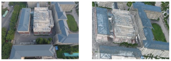
Figure 1.
An example of 3D reconstruction: (left) real image, (right) 3D model: point clouds.
Three-dimensional reconstruction methods are categorically divided into traditional and learning-based types, in which classification is based on the utilization of neural networks. Furthermore, based on their approach to acquiring scene information, they can be further categorized into active and passive reconstruction methods [3]. An active 3D reconstruction method scans a target through a 3D scanning device, followed by calculating the depth information of the object and obtaining point cloud data, which are used to restore the 3D model of the target. The main steps are data registration, point cloud data pre-processing, segmentation, and triangle meshing [4]. At present, widely adopted active methods encompass structured light-based 3D reconstruction [5,6], reconstruction from 3D laser scanning data [7], shadow detection [8,9], time of flight (TOF) [10,11], photometric stereo [12,13,14,15], and Kinect methods [16]. Structured light-based reconstruction methods emit specific light waves through the corresponding equipment and obtain information about the changes in light on the surface of an object. The data are then employed to calculate the 3D information, such as the surface depth of the object, so that a 3D model of the object can be reconstructed. Laser-scanning reconstruction uses the time difference between an emitted and returned laser to calculate the distance from an object’s surface to the scanner in order to reconstruct a 3D model. Passive 3D reconstruction is used to reconstruct a 3D model of an object through images collected using cameras. Since the images do not contain depth information about the object, 3D reconstruction can only be completed by predicting the surface depth of the object through geometric principles (Figure 2).
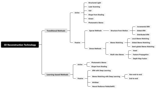
Figure 2.
Classification of 3D reconstruction technology.
Active methods, such as laser scanning, while capable of obtaining the precise depth information of objects, have their limitations. Firstly, their scanning equipment is typically expensive, bulky, and not affordable for the average research facility. Secondly, these scanning devices often rely on emitting and receiving light waves to calculate distances, making them susceptible to uncontrollable factors, such as lighting conditions in the environment. Consequently, they are usually more suitable for the 3D reconstruction of small objects and may not be ideal for large-scale scenes. Therefore, the focus has shifted toward passive methods that are reliant on camera images.
The remainder of this article is organized as follows: Section 2 introduces 3D reconstruction methods based on traditional methods. In Section 3, 3D reconstruction methods based on deep learning are presented. Section 4 provides a list of datasets and evaluation metrics for large-scale scenes. Finally, the challenges and outlook are provided in Section 5, and conclusions are drawn in Section 6.
2. Traditional Methods
In traditional passive reconstruction methods, the initial stage involves detecting and matching feature points in images, followed by associating corresponding points across multiple images for subsequent camera pose estimation and point cloud reconstruction. A typical pipeline of 3D reconstruction is shown in Figure 3. It is worth noting that, in Figure 3, the final step shows a mesh reconstruction. However, this article exclusively focuses on the generation of point clouds, and therefore, mesh reconstruction will not be introduced. This section presents an overview of the advancements in point cloud reconstruction techniques, including structure from motion (SfM) for sparse reconstruction, stereo matching, and multi-view stereo (MVS) for dense reconstruction.
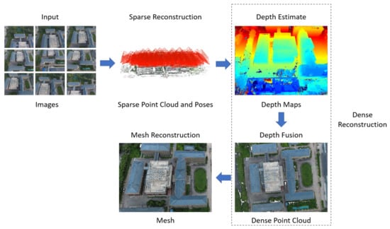
Figure 3.
A typical pipeline of 3D reconstruction. Step 1: Input multi-view images. Step 2: Use SfM to compute camera poses and reconstruct sparse point clouds. Step 3: Estimate depth using MVS. Step 4: Obtain a dense point cloud via depth fusion. Finally, obtain the mesh through mesh reconstruction.
2.1. Sparse Reconstruction: SfM
Structure from motion (SfM) is a technique that automatically recovers camera parameters and a 3D scene’s structure from multiple images or video sequences. SfM uses cameras’ motion trajectories to estimate camera parameters. By capturing images from different viewpoints, the camera’s position information and motion trajectory are computed. Subsequently, a 3D point cloud is generated in the spatial coordinate system. Existing SfM methods can be categorized into incremental, distributed, and global approaches according to the different methods for estimating the initial values of unknown parameters.
2.1.1. Incremental SfM
Incremental SfM [17], which involves selecting image pairs and reconstructing sparse point clouds, is currently the most widely used method. Photo Tourism, which was proposed by Snavley et al. [18], is the earliest incremental SfM system. It first selects a pair of images to compute the camera poses and reconstruct a partial scene. Then, it gradually adds new images and adjusts the previously computed camera poses and a scene model to obtain camera poses and scene information (Figure 4). Recently, a significant number of incremental SfM methods have been introduced, such as [19], EC-SfM [20], and AdaSfM [21].
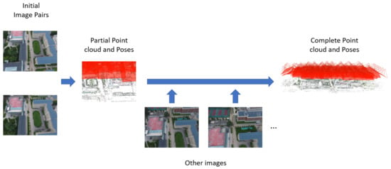
Figure 4.
An overview of incremental SfM. First, an initial image pair is selected to compute the camera poses and reconstruct a partial scene; then, gradually new images are gradually added to compute the complete point cloud.
In 2012, Moulon et al. [22] proposed Adaptive SfM (ASFM), an adaptive threshold estimation method that eliminates the need for manually setting hyperparameters. Due to the presence of noise and drift in pose and 3D point estimation, it is necessary to optimize the camera poses using the bundle adjustment (BA) algorithm after incorporating a certain number of new image pairs. In 2013, Wu et al. introduced VisualSFM [23], which improved the matching speed through a preemptive feature matching strategy and accelerated sparse reconstruction using a local–global bundle-adjustment technique. When the number of cameras increases, optimization is performed only on local images, and when the overall model reaches a certain scale, optimization is applied to all images, thus improving the reconstruction speed. In 2016, Schönberger et al. [24] integrated the classical SfM methods and made individual improvements to several key steps, such as geometric rectification, view selection, triangulation, and bundle adjustment, which were consolidated into COLMAP.
When reconstructing large-scale scenes using incremental SfM, errors accumulate as the number of images increases, leading to scene drift and time-consuming and repetitive bundle adjustments. Therefore, the initial incremental SfM approach is not ideal for large-scale outdoor scene reconstruction. In 2017, Zhu et al. [25] proposed a camera-clustering algorithm that divided the original SfM problem into sub-SfM problems for multiple clusters. For each cluster, a local incremental SfM algorithm was applied to obtain local camera poses, which were then incorporated into a global motion-averaging framework. Finally, the corresponding partial reconstructions were merged to improve the accuracy of large-scale incremental SfM, particularly in camera registration. In 2018, Qu et al. [26] proposed a fast outdoor-scene-reconstruction algorithm for drone images. They first used principal component analysis to select key drone images and create an image queue. Incremental SfM was then applied to compute the queue images, and new key images were selected and added to the queue. This enabled the use of incremental SfM for large-scale outdoor scene reconstruction. In 2019, Duan et al. [27] combined the graph optimization theory with incremental SfM. When constructing the graph optimization model, they used the sum of the squared reprojection errors as the cost function for optimization, aiming to reduce errors. Liu et al. [28] proposed a linear incremental SfM system for the large-scale 3D reconstruction of oblique photography scenes. They addressed the presence of many pure rotational image pairs in oblique photography data using bundle adjustment and outlier filtering to develop a new strategy for selecting initial image pairs. They also reduced cumulative errors by combining local bundle adjustment, local outlier filtering, and local re-triangulation methods. Additionally, the conjugate gradient method was employed to achieve a reconstruction speed that was close to linear speed. In 2020, Cui et al. [29] introduced a new SfM system. This system used track selection and camera prioritization to improve the robustness and efficiency of incremental SfM and make the datasets of large-scale scenes useful in SfM.
The main drawbacks of incremental SfM are as follows:
- Sensitivity to the selection of initial image pairs, which limits the quality of reconstruction to the initial pairs chosen.
- The accumulation of errors as new images are added, resulting in the scene-drift phenomenon.
- Incremental SfM is an iterative process where each image undergoes bundle adjustment optimization, leading to a significant number of redundant computations and lower reconstruction efficiency.
2.1.2. Global SfM
Global SfM encompasses the estimation of global camera rotations, positions, and point cloud generation. In contrast to incremental SfM, which processes images one by one, global SfM takes all of the images as input and performs bundle adjustment optimization only once, significantly improving the reconstruction speed. It evenly distributes errors and avoids error accumulation, resulting in higher reconstruction accuracy. It was first proposed by Sturm et al. [30]. In 2011, Crandall et al. [31] introduced a global approach based on Markov random fields. Hartley et al. [32] proposed the Weiszfeld algorithm based on the L1 norm to estimate camera rotations in the global SfM pipeline, achieving fast and robust results. In 2014, Wilson et al. [33] presented a 1D SfM method, which mapped the translation problem to a one-dimensional space, removed outliers, and then estimated global positions using non-convex optimization equations to reduce scene graph mismatches and improve the accuracy of position estimation. In 2015, Sweeney et al. [34] utilized the cycle-consistent optimization of a scene graph’s fundamental matrix to enhance the accuracy of camera pose estimation for image pairs. Cui et al. [35] proposed a novel global SfM method that optimized the solution process with auxiliary information, enabling it to handle various types of data.
However, global SfM may not yield satisfactory results for large-scale scenes due to the varying inter-camera correlations. In 2018, Zhu et al. [36] introduced a distributed framework for global SfM based on nested decomposition. They segmented the initial camera distribution map and iteratively optimized multiple segmented maps to improve local motion averages. Then, they optimized the connections between the sub-distribution maps to enhance global motion averaging, thereby improving global SfM reconstruction in large-scale scenes. In 2022, Pang [37] proposed a segmented SfM algorithm based on global SfM for the UAV-based reconstruction of outdoor scenes. The algorithm grouped UAV images based on latitude and longitude, extracted and matched features while removing mismatches, performed global SfM for each image group to obtain camera poses and sparse point clouds, merged point clouds, optimized scene spatial points and camera poses according to the grouping order, and finally performed global SfM on the merged data to obtain the point cloud of the entire large scene. Yu et al. [38] presented a robust global SfM algorithm for UAV-based 3D reconstruction. They combined rotation averaging from Lie algebra, the L1 norm, and least-squares principles to propose the L1-IRLS algorithm for computing the rotation parameters of UAV images, and they also incorporated GPS data into bundle adjustment to obtain high-precision point cloud data.
The main advantages of global SfM are as follows:
- Global SfM aims to optimize the camera poses and 3D scene structure simultaneously, ensuring that the entire reconstruction is globally consistent. This results in more accurate and reliable reconstructions.
- Global SfM typically employs optimization techniques such as global bundle adjustment, allowing it to provide high-precision estimates of camera parameters and 3D point clouds.
- Global SfM is typically suitable for large-scale scenes.
The main disadvantages of global SfM are as follows:
- Global SfM methods are computationally intensive and may require significant amounts of time and computational resources, especially for large datasets with many images and 3D points.
- The global camera position estimation results are unstable.
- Global SfM can be sensitive to outliers in the data. If there are incorrect correspondences or noisy measurements, they can have a significant impact on the global optimization process.
2.1.3. Distributed SfM
Although incremental SfM has advantages in robustness and accuracy, its efficiency is not high enough. Additionally, with the accumulation of errors, the scene structure is likely to exhibit drift in large-scale scene reconstruction. Global SfM is more efficient than the incremental approach; however, it is sensitive to outliers. In 2017, Cui et al. [39] proposed a distributed SfM method that combined incremental and global approaches. It used the incremental SfM method to compute camera positions for each additional image, and the camera rotation matrices were computed using the global SfM method. Finally, a local bundle adjustment algorithm was applied to optimize the camera’s center positions and scene 3D coordinates, thereby improving the reconstruction speed while ensuring robustness. In 2021, Wang et al. [40] introduced a hybrid global SfM method for estimating global rotations and translations at the same time. Distributed SfM combines the advantages of both methods to some extent.
2.2. Dense Reconstruction: Stereo Matching and MVS
2.2.1. Stereo Matching
Derived from the human binocular vision system [41], binocular vision imitates the principles of human vision to obtain a vast amount of three-dimensional data. It captures left and right images from different perspectives using two identical cameras at the same location. By utilizing the disparity formed from the two images, the depth of each pixel can be obtained. The process can be divided into four main steps: camera calibration, image rectification, stereo matching, and 3D reconstruction calculation [42]. Stereo matching, in particular, is the foundational and crucial step in binocular vision reconstruction.
Stereo matching aims to find corresponding pixels between two images captured using left and right cameras, calculates the corresponding disparity values, and then uses the principles of triangle similarity to obtain the depth information between objects and the cameras. However, challenges in improving the matching accuracy arise due to factors such as uneven illumination, occlusion, blurring, and noise [43]. The matching process mainly consists of four steps: matching cost calculation, matching cost aggregation, disparity calculation, and disparity refinement [44] (Figure 5). Additionally, to enhance accuracy, constraints such as the epipolar, uniqueness, disparity–continuity, ordering–consistency, and similarity constraints are employed to simplify the search process [45]. Based on these constraint methods, stereo matching algorithms can be classified into global, local, and semi-global matching methods (SGMs) [46].

Figure 5.
Workflow of stereo matching. First, the noise is reduced through image filtering, images are normalized, and image features are extracted. Then, the cost is computed, such as through the absolute differences in pixels between the images in an image pair. Finally, the disparity maps are computed, and the disparity map is refined.
Local Matching Method
Local matching methods in stereo vision rely on local constraints, such as windows, features, and phases, to perform matching, and they primarily utilize grayscale information from images. These methods determine disparities by establishing correspondences between the grayscale values of a given pixel and a small neighborhood of pixels. Currently, fixed-window [47], adaptive-window [48], and multi-window [49] algorithms are the main focus of research in window-based matching. While local matching algorithms can rapidly generate disparity maps, their accuracy is limited, particularly in regions with low texture and discontinuous disparities. In 2006, Yoon et al. [50] introduced the adaptive support weight (ASW) approach, which assigns different support weights to each pixel based on color differences and pixel distances. This technique improves matching accuracy in low-texture regions. In 2008, Wang et al. [51] proposed cooperative competition between regions to minimize the matching costs through collaborative optimization. In 2011, Liu et al. [52] introduced a new similarity measurement function to replace the traditional sum of absolute differences (SAD) function. They also employed different window sizes for matching in various regions and developed a new matching algorithm based on SIFT features and Harris corner points, improving both matching accuracy and speed. In 2014, Zhong et al. [53] introduced smoothness constraints and performed image segmentation using color images. They used a large window to match initial seed points and then expanded them using a small window to obtain a disparity map, effectively reducing matching errors in discontinuous disparity regions. In 2016, Hamzah et al. [45] addressed the limitations of single cost metrics by combining the absolute difference (AD), gradient matching (GM), and census transform (CN) into an iterative guided filter (GF) that enhanced edge information in images. Additionally, they introduced graph-cut algorithms to enhance robustness in low-texture regions and discontinuous disparity regions.
Local matching methods are efficient and flexible, yet they lack a holistic understanding of the scene, which makes them prone to local optima.
Global Matching Method
Global stereo matching algorithms primarily utilize the complete pixel information in images and the disparity information of neighboring pixels to perform matching. They employ constraint conditions to create an energy function that integrates all of the pixels in the image, aiming to obtain as much global information as possible. Global stereo matching algorithms can optimize the energy function through methods such as dynamic programming, belief propagation, and graph cuts [54].
Dynamic programming matching algorithms have been established under the constraint of epipolar lines. Optimal point searching and matching along each epipolar line are performed using dynamic programming with the aim of minimizing the global energy function and obtaining a disparity map. However, since only the pixels along the horizontal epipolar lines are scanned, the resulting disparity map often exhibits noticeable striping artifacts [54]. In 2006, Sung et al. [55] proposed a multi-path dynamic programming matching algorithm, which introduced a new energy function that considered the correlation between epipolar lines and utilized edge information in the images to address the discontinuity caused by occlusion, resulting in more accurate disparity estimation at boundary positions and reducing striping artifacts. In 2009, Li et al. [56] utilized the scale-invariant feature transform (SIFT) to extract feature points from images and performed feature point matching using a nearest-neighbor search, effectively alleviating striping artifacts. In 2012, Hu et al. [57] proposed a single-directional four-connected tree search algorithm and improved the dynamic programming algorithm for disparity estimation in boundary regions, enhancing both the accuracy and the efficiency of disparity estimation in boundary areas.
Stereo matching algorithms based on confidence propagation are commonly formulated as Markov random fields. In these algorithms, each pixel acts as a network node containing two types of information: data information, which stores the disparity value, and message information, which represents the node’s information to be propagated. Confidence propagation occurs among four neighboring pixels, enabling messages to propagate effectively in low-texture regions and ensuring accurate disparity estimation [58]. This approach achieves high matching accuracy by individually matching pixels throughout the entire image. However, it is characterized by a low matching efficiency and a long computation time. To address this issue, Zhou et al. [59] proposed a parallel algorithm in 2011. This algorithm divides the image into distinct regions for parallel matching, and the results from each region are subsequently combined to enhance the overall matching efficiency.
In stereo matching, the estimation of a disparity map can be formulated as minimizing a global energy function. Graph-cut-based matching algorithms construct a network graph of an image, where the problem of minimizing the energy function is equivalent to finding the minimum cut of the graph. By identifying the optimal image segmentation set, the algorithm achieves a globally optimal disparity map [60]. However, graph-cut algorithms often suffer from inaccurate initial matching in low-texture regions and require the computation of template parameters for all segmentation regions, leading to poor matching results in low-texture and occluded areas, as well as long computation times. In 2007, Bleyer et al. [61] proposed an improved approach that aggregated initial disparity segments into a set of disparity layers. By minimizing a global cost function, the algorithm selected the optimal disparity layer, resulting in improved matching performance in large textureless regions. Lempitsky et al. [62] achieved significant improvements in speed by parallelizing the computation of optimal segmentation and subsequently fusing the results. In 2014, He et al. [63] addressed the issues of blurry boundaries and prone-to-error matching in low-texture regions. They employed a mean-shift algorithm for image segmentation, performed singular value decomposition to fit disparity planes, and applied clustering and merging to neighboring segmented regions, leading to enhanced matching efficiency and accuracy in low-texture and occluded areas.
Global matching methods incorporate the advantages of local matching methods and adopt the cost aggregation approach used in local optimal dense matching methods. They introduce regularization constraints to obtain more robust matching results, but they consume more computational time and memory resources. Additionally, compared to local matching methods, global matching methods more readily incorporate additional prior information as constraints, such as the prevalent planar structural information in urban scenes, thus further enhancing the refinement of reconstruction results.
Semi-Global Matching Method
Semi-global matching (SGM) [64] also adopts the concept of energy function minimization. However, unlike global matching methods, SGM transforms the optimization problem of two-dimensional images into one-dimensional optimization along multiple paths (i.e., scanline optimization). It aggregates costs along paths from multiple directions and uses the Winner Takes All (WTA) algorithm to calculate disparities, achieving a good balance between matching accuracy and computational cost. The census transform proposed by Zabih [65] is widely used in matching cost computation. This method has a simple structure but is heavily reliant on the central pixel of the local window and is sensitive to noise. In 2012, Hermann et al. [66] introduced a hierarchical iterative semi-global stereo matching algorithm, resulting in a significant improvement in speed. Rothermel et al. [67] proposed a method for adjusting the disparity search range based on an image pyramid matching strategy called tSGM. They utilized the previous disparity to derive the dynamic disparity search range for each current pixel. This further reduced memory consumption while enhancing computational accuracy. In 2016, Tao [68] proposed a multi-measure semi-global matching method, building upon previous research. This method improved and expanded aspects such as the choice of penalty coefficients, similarity measures, and disparity range adjustments in classic semi-global matching algorithms. Compared to the method in [67], it offered enhancements in terms of reconstruction completeness and accuracy. In 2017, Li et al. [69] used mutual information combined with grayscale and gradient information as the matching cost function to calculate the cost values. They employed multiple adaptive path aggregations to optimize the initial cost values. Finally, they applied methods such as a left–right consistency check to complete the optimization. Additionally, they further refined the matching results using peak filters. In 2018, Chai et al. [70] introduced a semi-global matching method based on a minimum spanning tree. This approach calculated the cost values between pixels along four planned paths and aggregated the costs in both the leaf node and root node directions. The algorithm resulted in fewer mismatched points near the image edges and provided a more accurate disparity map. In 2020, Wang et al. [71] used SURF to detect potential matching points in remote sensing stereo image pairs. This was performed to modify the path weights in different aggregation directions, improving the matching accuracy in areas with weak texture and discontinuous disparities. However, the SURF step introduced additional computational burdens. Shrivastava et al. [72] extended the traditional semi-global matching (SGM) pipeline architecture by processing multiple pixels in parallel with relaxed dependency constraints, which improved the algorithm’s efficiency. However, it led to significant accuracy losses. In 2021, Huang et al. [73] introduced weights during the census transform phase, enabling the accurate selection of reference pixel values for the central point. They also used a multi-scale aggregation strategy with guided filtering as the cost aggregation kernel, resulting in improved matching accuracy. However, this significantly increased the algorithm’s complexity, making it less suitable for parallel implementation. Zhao et al. [74] replaced the central pixel with the surrounding pixels of the census window during the transformation process, making it more robust and achieving good disparity results. In 2022, Lu et al. [75] employed a strategy involving downsampling and disparity skipping. They also introduced horizontal path weighting during aggregation. However, this approach introduced a new path weight parameter, increasing the computational complexity of cost aggregation.
The current semi-global stereo matching algorithms have made significant advancements in both accuracy and efficiency. However, they have not achieved a well-balanced trade-off between accuracy and efficiency.
2.2.2. Multi-View Stereo
When using SfM for scene reconstruction, the sparsity of feature matching points often leads to a sparse point cloud and unsatisfactory reconstruction results. To overcome this limitation, multi-view stereo (MVS) techniques are employed to enhance the reconstruction. MVS leverages the camera pose parameters from SfM in a scene to capture richer information. Moreover, the image rectification and stereo matching mentioned in Section 2.2 are used in MVS. The primary goal is to identify the most effective method of matching corresponding points across different images, thereby improving the density of the scene and enhancing the quality of the reconstruction (Figure 6). MVS can be implemented through three main methods: voxel-based reconstruction, feature propagation, and depth map fusion [76].
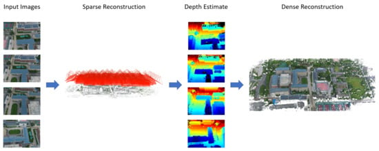
Figure 6.
Dense reconstruction based on MVS.
The voxel-based algorithm defines a spatial range—typically a cube—that encapsulates the entire scene to be reconstructed. This cube is then subdivided into smaller cubes, which are known as voxels. By assigning occupancy values to the voxels based on scene characteristics, such as filling voxels in occupied regions and leaving others unfilled in unoccupied regions, a 3D model of the object can be obtained [77]. However, this algorithm has limitations. Firstly, it requires an initial determination of a fixed spatial range, which limits its ability to reconstruct objects beyond that range. Secondly, the algorithm’s complexity restricts the number of subdivisions, resulting in relatively lower object resolution.
The feature propagation method involves generating surface slices and an initial point cloud based on initial feature points. These feature points are projected onto images and propagated to the surrounding areas. Finally, surface slices are used to cover the scene surface for 3D reconstruction. Each surface slice can be visualized as a rectangle with information such as its center and surface normal vector. By estimating surface slices and ensuring the complete coverage of the scene, an accurate and dense point cloud structure can be obtained [78]. In 2010, Furukawa proposed a popular feature-propagation-based MVS algorithm called PMVS [79].
The depth map fusion method is the most commonly used and effective approach in multi-view stereo vision. It typically involves four steps: reference image selection, depth map estimation, depth map refinement, and depth map fusion [80]. Estimating depth maps is a critical step in multi-view stereo reconstruction, where an appropriate depth value is assigned to each pixel in the image. This estimation is achieved by maximizing the photometric consistency between an image and a corresponding window in the reference image centered at that pixel (Figure 7). Common metrics for photometric consistency include the mean absolute difference (MAD), the sum of squared differences (SSD), the sum of absolute differences (SAD), and normalized cross-correlation (NCC) [52].

Figure 7.
Flowchart of depth estimation. The cost volume of selecting a candidate set is generated using certain criteria, such as variance. All cost volumes are aggregated, and the depth is estimated using the cost volume. Finally, depth maps are obtained after optimization.
3. Learning-Based Methods
Traditional 3D reconstruction methods have been widely applied in various industries and in daily life. While traditional 3D reconstruction methods still dominate the research field, an increasing number of researchers are starting to focus on using deep learning to explore 3D reconstruction, or in other words, the intersection and fusion of the two approaches. With the development of deep learning, convolutional neural networks (CNNs) have been extensively used in computer vision. CNNs have significant advantages in image processing, as they can directly take images as inputs, avoiding the complex processes of feature extraction and data reconstruction in traditional image processing algorithms. Although deep-learning-based 3D reconstruction methods have been developed relatively recently, they have progressed rapidly. Deep learning has made significant advancements in the research of 3D reconstruction. What roles can deep learning play in 3D reconstruction? Initially, deep learning can provide new insights into the optimization of the performance of traditional reconstruction methods, such as Code SLAM [81]. This approach employs deep learning methods to extract multiple basis functions from a single image, using neural networks to represent the depth of a scene. These representations can greatly simplify the optimization problems present in traditional geometric methods. Secondly, the fusion of deep-learning-based reconstruction algorithms with traditional 3D reconstruction algorithms leverages the complementary strengths of both approaches. Furthermore, deep learning can be used to mimic human vision and directly reconstruct 3D models. Since humans can perform 3D reconstruction based on their brains rather than strict geometric calculations, it is theoretically feasible to use deep learning methods directly. It is essential to note that, in some research, certain methods aim to perform 3D reconstruction directly from a single image. In theory, a single image lacks the 3D information of an object and is, thus, unable to recover depth information. However, humans can make reasonable estimates of an object’s distance based on experience, which adds some plausibility to such methods.
This section will introduce the applications of deep learning in traditional methods such as structure from motion, stereo matching, and multi-view stereo vision, as well as in the novel approach of neural-radiance-field-based 3D reconstruction.
3.1. SfM with Deep Learning
The combination of deep learning and SfM enables the efficient estimation of camera poses and scene depth due to the high accuracy and efficiency of feature extraction and matching in CNNs [82]. In 2017, Zhou et al. [83] achieved good results by utilizing unsupervised photometric error minimization. They employed two jointly trained CNNs to predict depth maps and camera motion. Ummenhofer et al. [84] utilized optical flow features to estimate scene depth and camera motion, improving the generalization capabilities in unfamiliar scenes. In 2018, Wang et al. [85] incorporated a multi-view geometry constraint between depth and motion. They used a CNN to estimate the scene depth and a differentiable module to compute camera motion. In 2019, Tang et al. [86] proposed a deep learning framework called BA-Net (Bundle Adjustment Network). The core of the network was a differentiable bundle adjustment layer that predicted both the scene depth and camera motion based on CNN features. It emphasized the incorporation of multi-view geometric constraints, enabling the reconstruction of an arbitrary number of images.
3.2. Stereo Matching with Deep Learning
In 2015, LeCun et al. [87] introduced the use of convolutional neural networks (CNNs) for extracting image features in cost computation. Furthermore, they presented cost aggregation with a cross-cost consistency check. This approach eliminated erroneous matching areas, marking the emergence of deep learning as a significant technique in stereo matching.
3.2.1. Non-End-to-End Methods
The image networks used for stereo matching can be categorized into three main types: pyramid networks [88], Siamese networks [89], and generative adversarial networks (GANs) [90].
In 2018, Chang et al. [91] incorporated a pyramid pooling module during the feature extraction stage. They utilized multi-scale analysis and a 3D-CNN structure to effectively address issues such as vanishing and exploding gradients, achieving favorable outcomes even under challenging conditions, such as weak textures, occlusion, and non-uniform illumination. There are also some other related works, such as CREStereo [92], ACVNet [93], and NIG [94].
Siamese networks, pioneered by Bromley et al. [89], consist of two weight-sharing CNNs that take the left and right images as inputs. Feature vectors are extracted from these images, and the L1 distance between the feature vectors is measured to estimate the similarity between the images (Figure 8). MC-CNN [87] is a classic example of a network based on Siamese networks. Zagoruyko et al. [95] enhanced the original Siamese network by incorporating the ReLU function and smaller convolutional kernels, thereby deepening the convolutional layers and improving the matching accuracy. In 2018, Khamis [96] utilized a Siamese network to extract features from left and right images. They first computed a disparity map using low-resolution cost convolution and then introduced a hierarchical refinement network to capture high-frequency details. The guidance of a color input facilitated the generation of high-quality boundaries.
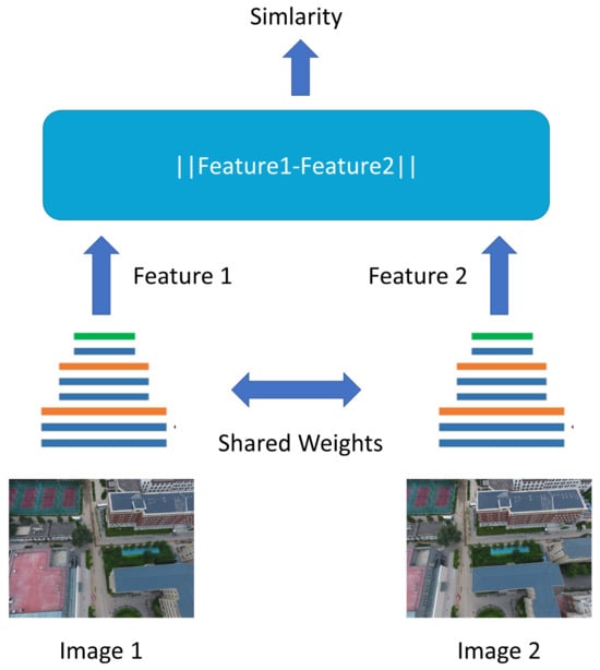
Figure 8.
Architecture of Siamese networks. Two CNNs with shared weights are used to extract image features.
Generative adversarial networks (GANs), which were proposed by Luo et al. [90], consist of a generator model and a discriminator model. The generator model learns the features of input data and generates images similar to the input images, while the discriminator model continuously distinguishes between the generated images and the original images until a Nash equilibrium is reached (Figure 9). In 2018, Pilzer et al. [97] presented a GAN framework based on binocular vision. It comprised two generator sub-networks and one discriminator network. The two generator networks were used in adversarial learning to train the reconstruction of disparity maps. Through mutual constraints and supervision, they generated disparity maps from two different viewpoints, which were then fused to produce the final data. Experiments demonstrated that this unsupervised model achieved good results under non-uniform lighting conditions. Lore et al. [98] proposed a deep convolutional generative model that obtained multiple depth maps from neighboring frames, further enhancing the quality of depth maps in occluded areas. In 2019, Matias et al. [99] used a generative model to handle occluded areas and achieved satisfactory disparity results.
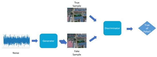
Figure 9.
Architecture of a GAN: generator: generates fake samples using noise and image features; discriminator: distinguishes true samples and fake samples generated by the generator.
3.2.2. End-to-End Methods
The deep-learning-based non-end-to-end stereo matching methods mentioned in Section 3.2.1 essentially do not deviate from the framework of traditional methods. In general, they still require the addition of hand-designed regularization functions or post-disparity processing steps. This means that non-end-to-end stereo matching methods have the drawbacks of high computational complexity and low time efficiency, and they have not resolved the issues present in traditional stereo matching methods, such as limited receptive fields and a lack of image contextual information. In 2016, Mayer et al. [100] successfully introduced an end-to-end network structure into the stereo matching task for the first time and achieved good results. The design of more efficient end-to-end stereo matching networks has gradually become a research trend in stereo matching.
Current end-to-end stereo matching networks take left and right views as inputs. After feature extraction using convolutional modules with shared weights, they construct a cost volume using either correlation or concatenation operations. Finally, different convolution operations are applied based on the dimensions of the cost volume to regress the disparity map. End-to-end stereo matching networks can be categorized into two approaches: those based on 3D cost volumes and those based on 4D cost volumes according to the dimensions of the cost volume. In this article, the focus is on 4D cost volumes.
In contrast to architectures inspired by traditional neural network models, end-to-end stereo matching network architectures based on 4D cost volumes are specifically designed for the stereo matching task. In this architecture, the network no longer performs dimension reduction on the features, allowing the cost volume to retain more image geometry and contextual information. In 2017, Kendall et al. [101] proposed a novel deep disparity learning network named GCNet, which creatively introduced a 4D cost volume and, for the first time, utilized 3D convolutions in the regularization module to integrate contextual information from the 4D cost volume. This pioneering approach established a 3D network structure that was specifically designed for stereo matching (Figure 10). It first used weight-sharing 2D convolutional layers to separately extract high-dimensional features from the left and right images. At this stage, downsampling was performed to reduce the original resolution by half, which helped reduce the memory requirements. Then, the left feature map and the corresponding channel of the right feature map were combined pixel-wise along the disparity dimension to create a 4D cost volume. After that, it utilized an encoding–decoding module consisting of multi-scale 3D convolutions and deconvolutions to regularize the cost volume, resulting in a cost volume tensor. Finally, the cost volume was regressed with a differentiable Soft ArgMax to obtain the disparity map. GC-Net was considered state of the art due to its 4D (height, width, disparity, and feature channels) volume. In 2018, Chang et al. [91] proposed the pyramid stereo matching network (PSMNet). It was primarily composed of a spatial pyramid pooling (SPP) module and a stack of hourglass-shaped 3D CNN modules. The pyramid pooling module was responsible for extracting multi-scale features to make full use of global contextual information, while the stacked hourglass 3D encoder–decoder structure regularized the 4D cost volume to provide disparity predictions. However, due to the inherent information loss in the pooling operations at different scales within the SPP module, PSMNet exhibited lower matching accuracy in image regions that contained a significant amount of fine detail information, such as object edges.

Figure 10.
Architecture of GC-Net [101]. Step 1: Weight-sharing 2D convolution is used to extract image features and downsample. Step 2: The 4D cost volume is created by combining left and right images’ feature maps. Step 3: The cost volume is regularized through multi-scale 3D convolution and 3D deconvolution. Step 4: The cost volume is regressed with a differentiable Soft ArgMax, and a disparity map is obtained.
Although end-to-end networks based on 4D cost volumes achieve good matching results, the computational complexity of the 3D convolutional structure itself results in high costs in terms of both storage resources and computation time. In 2019, Wang et al. [102] introduced a three-stage disparity estimation network called AnyNet, which used a coarse-to-fine strategy. Firstly, the network constructed a low-resolution 4D cost volume using low-resolution feature maps as input. Then, it searched within a smaller disparity range using 3D convolutions to obtain a low-resolution disparity map. Finally, it upsampled the low-resolution disparity map to obtain a high-resolution disparity map. This method was progressive, allowing for stopping at any time to obtain a coarser disparity map, thereby trading matching speed for accuracy. Zhang et al. [103] proposed GA-Net, which replaced many 3D convolutional layers in the regularization module with semi-global aggregation (SGA) layers and local guided aggregation (LGA) layers. SGA is a differentiable approximation of cost aggregation methods used in SGM, and the penalty coefficient is learned by the network instead of being determined by prior knowledge. This provides better adaptability and flexibility for different regions of an image. The LGA layer is appended at the end of the network to aggregate local costs with the aim of refining disparity near thin structures and object edges.
3.3. MVS with Deep Learning
In 2018, Yao et al. pioneered the combination of convolutional neural networks and MVS, resulting in the development of MVSNet [104]. They extracted image features using a CNN, utilized a differentiable homography matrix to construct a cost volume, and regularized the cost volume using 3D U-Net, enabling multi-view depth estimation (Figure 11). Building upon this work, Yao et al. [105] introduced RMVSNet (recurrent MVSNet) in 2019. By replacing the 3D CNN convolution in MVSNet with gated units, they achieved reduced memory consumption. Chen et al. [106] proposed PointMVSNet, which employed graph convolutional networks to refine the point cloud generated by MVSNet. Luo et al. [107] introduced P-MVSNet (Patchwise MVSNet), which significantly improved the accuracy and completeness of depth maps and reconstructed a point cloud through the application of the Patchwise approach. Xue et al. [108] proposed MVSCRF (MVS Conditional Random Field), which incorporated a conditional random field (CRF) module to enforce smoothness constraints on the depth map. This approach resulted in enhanced depth estimation. Yi et al. [109] presented PVA-MVSNet (Pixel View Adaptive MVSNet), which generated depth estimation with higher confidence by adaptively aggregating views at both the pixel and voxel levels. Yu et al. [110] introduced Fast-MVSNet, which utilized sparse cost volume and Gauss–Newton layers to enhance the runtime speed of MVSNet. In 2020, Gu et al. [111] introduced Cascade MVSNet, a redesigned model that encoded features from different scales using an image feature pyramid in a cascading manner. This approach not only saved memory resources but also improved MVS speed and accuracy. Yang et al. [112] proposed CVP-MVSNet (Cost–Volume Pyramid MVSNet), which employed a pyramid-like cost–volume structure to adjust the depth map at different scales, from coarse to fine. Cheng et al. [113] developed a network that automatically adjusted the depth interval to avoid dense sampling and achieved high-precision depth estimation. Yan et al. [114] introduced D2HC-RMVSNet (Dense Hybrid RMVSNet), a high-density hybrid recursive multi-view stereo network that incorporated dynamic consistency checks, yielding excellent results while significantly reducing memory consumption. Liu et al. [115] proposed RED-Net. It introduced a recurrent encoder–decoder (RED) architecture for sequential regularization of cost volume, achieving higher efficiency and accuracy while maintaining resolution, which was beneficial for large-scale reconstruction. In 2022, a significant number of works based on some helpful modules in computer vision, such as attention and transformers, were introduced [116,117,118,119,120]. In 2023, Zhang et al. [121] proposed DSC-MVSNet, which used separable convolution based on depth and attention modules to regularize the cost volume. Zhang et al. [122] proposed vis-MVSNet, which estimated matching uncertainty and integrated pixel-level occlusion information within the network to enhance depth estimation accuracy in scenes with severe occlusions. There were also more studies on MVSNet (Figure 12), such as MS-REDNet [123], AACVP-MVSNet [124], Sat-MVSF [125], RA-MVSNet [126], M3VSNet [127], and Epp-MVSNet [128].
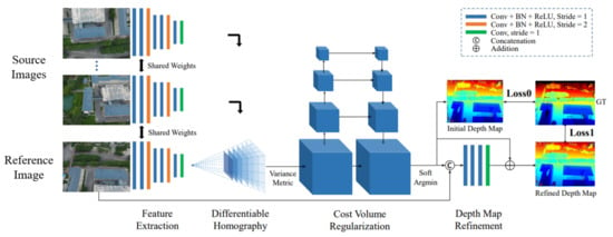
Figure 11.
Overview of MVSNet [104]. Image features are extracted by multiple CNNs that share weights. Then, a differentiable homography matrix and variance metric are utilized to generate the cost volume, and a 3D U-Net is used to regularize the cost volume. Finally, depth maps are estimated and refined with the regularized probability volume and a reference image.

Figure 12.
Chronological overview of MVSNet methods [104,105,106,107,108,109,110,111,112,113,114,115,116,117,118,119,120,121,122,123,124,125,126,127,128].
3.4. Neural Radiance Fields
In 2020, a groundbreaking scene-rendering technique called Neural Radiance Fields (NeRF) was introduced by Ben et al. [129]. NeRF is an end-to-end learning framework that leverages the spatial coordinates of objects and camera poses as input, and a multi-layer perceptron (MLP) network is utilized to simulate a neural field. This neural field represents a scalar property, such as opacity, of the object in a specific direction. By tracing rays through the scene and integrating colors based on the rays and opacity, NeRF generates high-quality images or videos from novel viewpoints (Figure 13). Building upon NeRF, Zhang et al. [130] proposed NeRF++, which addresses the potential shape–illumination ambiguity. It acknowledges that, while the geometric representation of space in an NeRF model trained on a scene’s dataset could be incorrect, it can still render accurate results on the training samples. However, for unseen views, incorrect shapes may result in imperfect generalization. NeRF++ tackles this challenge and resolves the parameterization issue when applying NeRF to unbounded 360° scenes. This enhancement allows for better capturing of objects in large-scale, unbounded 3D scenes. Although NeRF itself does not possess inherent 3D object reconstruction capabilities, modifications and variants that incorporate geometric constraints have been developed. These NeRF-based methods enable the end-to-end reconstruction of 3D models of objects or scenes by integrating geometric constraints into the learning framework. There have been a significant number of studies on NeRF in recent years (Figure 14), such as DeRF [131], depth-supervised NeRF [132], Mip-NeRF [133], Mip-NeRF 360 [134], Ha-NeRF [135], DynIBaR [136], MRVM-NeRF [137], MVSNeRF [138], PointNeRF [139], and ManhattanNeRF [140].

Figure 13.
A pipeline of NeRF. The 5D information, including the 3D position of the pixel of the target scene and the view direction observing the scene, is input into an MLP. Then, the color and density information about the pixel are output. Finally, the volume is rendered using loss functions.

Figure 14.
Chronological overview of NeRF methods [129,130,131,132,133,134,135,136,137,138,139,140,141,142,143,144,145,146,147,148,149,150,151,152,153,154,155,156,157,158,159].
When facing large-scale outdoor scenes, the main challenges that need to be addressed are as follows:
- Accurate six-DoF camera pose estimation;
- Normalization of lighting conditions to avoid overexposed scenes;
- Handling open outdoor scenes and dynamic objects;
- Striking a balance between accuracy and computational efficiency.
To obtain more accurate camera poses, in 2021, Lin et al. [141] proposed I-NeRF, which inverted the training of NeRF by using a pre-trained model to learn precise camera poses. Lin et al. [142] introduced BA-NeRF, which could optimize pixel-level loss even with noisy camera poses by computing the difference between the projected results of rotated camera poses and the given camera pose. They also incorporated an annealing mechanism in the position-encoding module, gradually introducing high-frequency components during the training process, resulting in accurate and stable reconstruction results.
To address the issue of lighting, in 2021, Ricardo et al. [143] introduced two new encoding layers: appearance embedding, which modeled the static appearance of the scene, and transient embedding, which modeled transient factors and uncertainties, such as occlusions. In 2022, by learning these embeddings, they achieved a control mechanism for adjusting a scene’s lighting. Darius et al. [144] proposed the ADOP (approximate differentiable one-pixel point) rendering method, which incorporated a camera-processing pipeline to rasterize a point cloud, and they fed it into a CNN for convolution, resulting in high-dynamic-range images. They then utilized traditional differentiable image processing techniques, such as lighting compensation, and trained the network to learn the corresponding weights, achieving fine-grained modeling. Ben et al. [145] discovered the issue of inconsistent noise between RGB-processed images and the original data. They proposed training NeRF on the original images before RGB processing and obtaining RGB images using image processing methods. This approach resulted in more consistent and uniform lighting. This approach leveraged the implicit alignment capabilities of NeRF and utilized the consensus relationships between multiple shots to complement each other’s information. Rudnev et al. [146] introduced the NeRF-OSR method, which learned an implicit neural scene representation by decomposing the scene into spatial occupancy, illumination, shadow, and diffuse reflectance. This method supported the meaningful editing of scene lighting and camera viewpoints simultaneously and in conjunction with semantics.
When modeling open scenes and dynamic objects and when modeling outdoor scenes with NeRF, neglecting the far scene can result in background errors, while modeling it can lead to a reduced resolution in the foreground due to scale issues. NeRF++, which was created by Zhang et al. [130], addressed this problem by proposing a simplified inverse sphere-parameterization method for free viewpoint synthesis. The scene space was divided into two volumes: an inner unit sphere, representing the foreground and all cameras, and an outer volume, represented by an inverted sphere that covered the complementary portion of the inner volume. The inner volume contained the foreground and all cameras, while the outer volume represented the remaining environment, and both parts were rendered using separate NeRF models. In 2021, Julian et al. [147] introduced the neural scene graph (NSG) method for dynamic rigid objects. It treated the background as the root node and the moving objects as the foreground (neighbor nodes). The relationships between poses and scaling factors were used to create edges in the associated graph, and intersections between rays and the 3D bounding boxes of the objects were verified along the edges. If there was an intersection, the rays were bent, and modeling was performed separately for the inside and outside of the detection box to achieve consistent foreground–background images. Paul et al. [148] proposed TransNeRF based on transfer learning, where they first used a generative adversarial network (GAN) called GLO [149] to learn and model dynamic objects based on NeRF-W [143]. Then, a pre-trained NeRF++ was used as the MLP module in the network (Figure 15). In 2022, Abhijit et al. [150] introduced Panoptic NeRF, which decomposed dynamic 3D scenes into a series of foreground and background elements, representing each foreground element with a separate NeRF model.
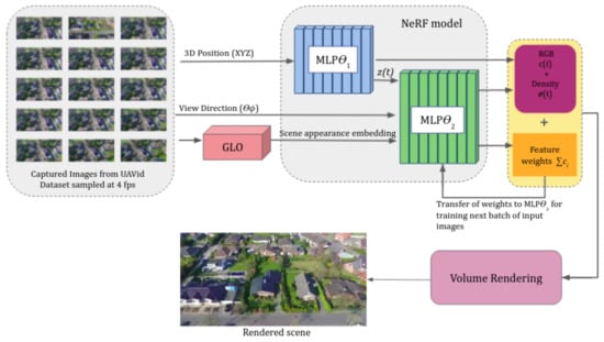
Figure 15.
Architecture of TransNeRF [148]. The 3D position is input into a color MLP to obtain color information and into the GLO module to generate a scene appearance embedding. The color information, view direction, and appearance embedding go through another density MLP to obtain the density information. Both of the MLPs come from an NeRF++ model, and the feature weights of the density MLP guide the training of the next batch of input images.
In terms of large-scale scenes, Haithem et al. [151] proposed Mega-NeRF for drone scenes, which employed a top-down 2D grid approach to divide the scene into multiple grids. The training data were then reorganized into each grid based on the intersections between camera rays and the scene, enabling individual NeRF models to be trained for each grid. They also introduced a new guided sampling method that sampled points only near the object’s surface, improving the rendering speed. In addition, improvements were made to NeRF++ by dividing the scene into foreground and background regions using ellipsoids. Taking advantage of the camera height measurements, rays were terminated near the ground to further refine the sampling range. Derksen et al. [152] introduced S-NeRF, which was the first application of Neural Radiance Fields to the reconstruction of 3D models from multi-view satellite images. It directly modeled direct sunlight and a local light field and learned the diffuse light, such as sky light, as a function of the sun’s position. This approach leveraged non-correlated effects in satellite images to generate realistic images under occlusion and changing lighting conditions. In 2022, Xu et al. [153] proposed BungeeNeRF, which used progressive learning to gradually refine the fitting of large-scale city-level 3D models, starting from the distant view and progressively capturing different levels of detail. Rematas et al. [154] introduced Urban Radiance Fields (URFs), which incorporated information from LiDAR point clouds to guide NeRF in reconstructing street-level scenes. Matthew et al. [155] proposed BlockNeRF, which divided large scenes based on prior map information. They created circular blocks centered around the projected points of the map’s blocks and trained a separate NeRF model for each block. By combining the outputs of multiple NeRF models, they obtained optimal results. Mari et al. [156] extended the work of S-NeRF by introducing a rational polynomial camera model to improve the robustness of the network to changing shadows and transient objects in satellite cameras. Huang et al. [157] took a traditional approach by assuming existing surface hypotheses for buildings. They introduced a new energy term to encourage roof preference and two additional hard constraints, explicitly obtaining the correct object topology and detail recovery based on LiDAR point clouds. In 2023, Zhang et al. [158] proposed GP-NeRF, which introduced a hybrid feature based on 3D hash grid features and multi-resolution plane features. They extracted the grid features and plane features separately and then combined them as inputs into NeRF for density prediction. The plane features were also separately input into the color-prediction MLP network, improving the reconstruction speed and accuracy of NeRF in large-scale outdoor scenes. Xu et al. [159] proposed Grid-NeRF, which combined feature grids and introduced a dual-branch structure with a grid branch and a NeRF branch trained in two stages. They captured scene information using a feature plane pyramid and input it into the shallow MLP network (grid branch) for the feature grid learning. The learned feature grid guided the NeRF branch to sample object surfaces, and the feature plane was bilinearly interpolated to predict the grid features of the sampled points. These features, along with positional encoding, were then input into the NeRF branch for rendering.
4. Datasets and Evaluation Metrics
According to the different types of target tasks, the datasets for 3D reconstruction can be also divided into different categories (Table 1). The datasets mentioned in this section are commonly used in corresponding tasks, which mainly include large-scale scenes. These datasets comprise high-resolution satellite images, low-altitude images captured by UAVs, and street-view images captured with handheld cameras in urban environments. They provide rich urban scenes, encompassing diverse architectural structures and land cover types, which are crucial for this research on large-scale 3D reconstruction. Additionally, the evaluation metrics depend on the reconstruction methods, which will be introduced in detail in this section.

Table 1.
Brief introduction to the datasets for the 3D reconstruction of large-scale or outdoor scenes.
4.1. Structure from Motion
4.1.1. Datasets
The BigSfM project contains a large number of SfM datasets that are mainly used for the reconstruction of large-scale outdoor scenes. It was proposed by Cornell University. These datasets are usually collected on the Internet, including multiple sets of city landmark images downloaded from Flickr and Google (Figure 16), such as Quad 6K [160], Dubrovnik6K [161], Rome16K [161], and the older NotreDame [18].
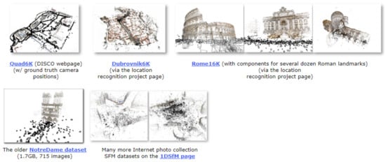
Figure 16.
Some famous and common datasets of the BigSfM project.
Quad6K: This dataset contains 6514 images of Cornell University’s Arts Quad; the geographic information from about 5000 images was recorded with the GPS receiver of the user’s own iPhone 3G, and the geographic information from 348 images was measured and recorded using high-precision GPS equipment.
Dubrovnik6K: This dataset contains 6844 images of landmarks in the city of Dubrovnik, and it consists of SIFT features, SfM models, and query images corresponding to SIFT features.
Rome 16K: This dataset contains 16,179 images of landmarks in Roman cities, and it consists of SIFT features, SfM models, and query images corresponding to SIFT features.
The older NotreDame: This dataset contains 715 images of Notre Dame.
4.1.2. Evaluation Metrics
SfM restores the sparse 3D structure in the case of unknown camera poses, and it is difficult for it to obtain the ground truth of a reconstruction, so indirect evaluation metrics are generally used to reflect the reconstruction quality. Therefore, the evaluation metrics of SfM are the number of registered images (Registered), the number of sparse point clouds (Points), the average length of the trajectory (Track), and the point cloud reprojection error (Reprojection Error).
- Registered: The more registered images there are, the more information is used in SfM reconstruction, which indirectly indicates the accurate reconstruction of the points because the reconstruction registration depends on the accuracy of the intermediate process points.
- Points: The more points there are in the sparse point cloud, the higher the degree of matching between the poses of the camera and the 2D points because the accuracy of triangulation depends on both of the above.
- Track: The number of 2D points corresponding to each 3D point. The longer the trajectory of the point, the more information is used, which indirectly means that the accuracy is high.
- Reprojection Error: The average distance error between the position of each 3D point projected to each frame with the poses and the position of the actual detected 2D point. The smaller the reprojection error, the higher the accuracy of the overall structure.
4.2. Stereo Matching
4.2.1. Datasets
WHU-Stereo [162]: This dataset is based on images of GF-7 and airborne LiDAR point clouds (Figure 17), including buildings and vegetation scenes in six cities in China: Shaoguan, Kunming, Yingde, Qichun, Wuhan, and Hengyang. There are 1757 image pairs with dense disparities.
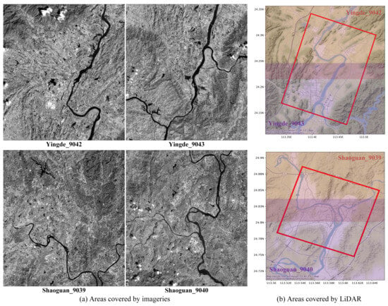
Figure 17.
Examples from the WHU-Stereo dataset. Areas covered by GF-7 satellite images of the cities of Yingde and Shaoguan (a) and approximate LiDAR data (b).
US3D [163]: This dataset contains two urban scenes from Jacksonville, Florida and Omaha, Nebraska. A total of 4292 image pairs with dense disparities were constructed from 26 panchromatic, visible-light, and near-infrared images of Jacksonville and 43 images of Omaha, and they were collected using WorldView-3 (Figure 18). However, since many of the image pairs were captured from the same area and taken at different times, there may be seasonal differences in the appearance of land cover.
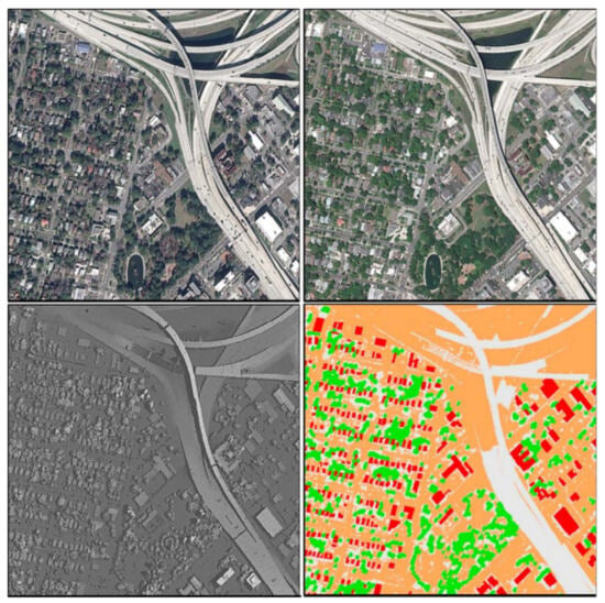
Figure 18.
Examples from the US3D dataset. Epipolar rectified images (top) with ground truth left disparities and semantic labels (bottom).
Satstereo [164]: Most of this dataset uses WorldView-3 images, and a small portion comes from WorldView-2. In addition to the dense disparity, it also builds masks and provides metadata for each image, but as with US3D, there are differences in the seasonal appearance of land cover due to the different acquisition times.
4.2.2. Evaluation Metrics
The main evaluation criteria for stereo matching algorithms are the disparity map’s accuracy and the time complexity. The evaluation metrics for the disparity map’s accuracy include the false matching rate, the mean absolute error (MAE), and the root mean square error (RMSE) [44].
- The false matching rate iswhere and are the respective pixel values of the generated disparity map and the real disparity map. is the evaluation threshold that one sets, and when the difference is greater than , the pixel is marked as a mismatched pixel. N is the total number of pixels in the disparity map.
- MAE:
- RMSE:
4.3. Multi-View Stereo
4.3.1. Datasets
ETH3D [165]: This dataset includes images captured with high-definition cameras and the ground truth of dense point clouds obtained with industrial laser scanners; it includes buildings, natural landscapes, indoor scenes, and industrial scenes (Figure 19). The data of the two modalities are aligned through an optimization algorithm.
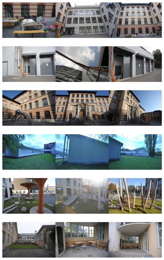
Figure 19.
Examples from the ETH3D dataset. Some high-resolution images of buildings and outdoor scenes.
Tanks and Temples [166]: This dataset involved the use of a high-definition camera to shoot videos of real scenes (Figure 20). The number of images in each scene is about 400, and the camera poses are unknown. The ground truth of the dense point cloud was obtained using an industrial laser scanner.
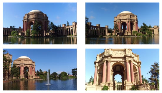
Figure 20.
Examples from Tanks and Temples dataset. Some high-resolution images of the palace scene.
Sensefly [167]: This is an outdoor scene dataset released by Sensefly, a light fixed-wing UAV company, and it includes schools, parks, cities, and other scenes, with RGB, multi-spectral, point cloud, and other data types (Figure 21).
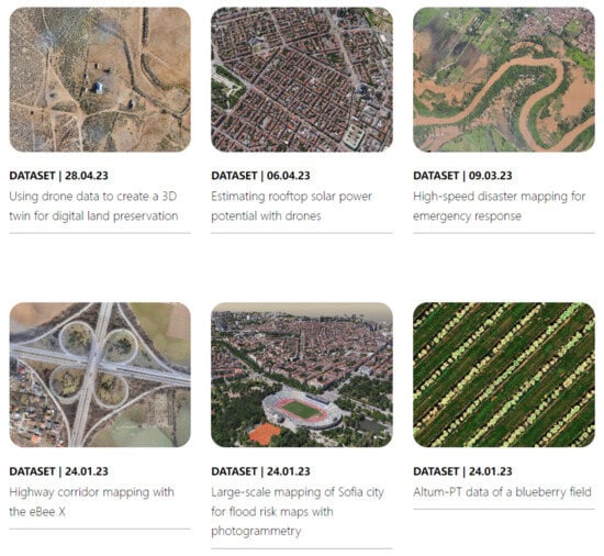
Figure 21.
Some typical examples from the dataset created by Sensefly, including cities, highways, blueberry fields, and other scenes.
BlendedMVS [168]: This dataset is a large-scale MVS dataset for generalized multi-view stereo networks. The dataset has a total of 17,000 MVS training samples, including 113 scenes, with buildings, sculptures, small objects, and so on. Additionally, there are 29 large scenes, 52 small scenes, and 32 scenes of sculptures (Figure 22).
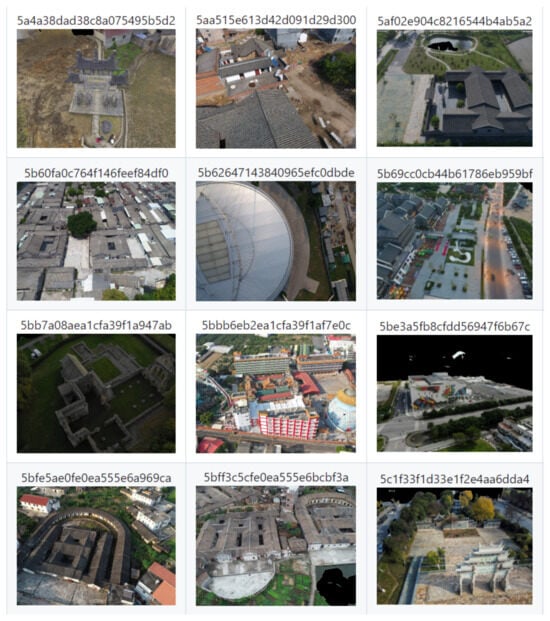
Figure 22.
Examples from the BlendedMVS dataset. High-resolution images of 12 large scenes from a total of 113 scenes.
4.3.2. Evaluation Metrics
The purpose of multi-view stereo vision is to estimate a dense 3D structure under the premise of knowing the camera poses. If the camera poses are unknown, it is necessary to estimate the camera poses first with SfM. The evaluation of the dense structures is generally based on a point cloud obtained using LiDAR or depth cameras. Some of the corresponding camera poses are directly acquired using a robotic arm during collection, such as in DTU [171], and some are estimated based on the collected depth, such as in ETH3D or Tanks and Temples. The evaluation metrics are the accuracy and completeness, as well as the F1-score, which balances the two. Additionally, some evaluation and visualization results for typical MVSNet models are shown in Table 2, Figure 23 and Figure 24.
- Accuracy: For each estimated 3D point, a true 3D point is found within a certain threshold, and the final matching ratio is the accuracy. It should be noted that, since the ground truth of the point cloud itself is incomplete, it is necessary to estimate the unobservable part of the ground truth first and ignore it when estimating the accuracy.
- Completeness: The nearest estimated 3D point is found within a certain threshold for each true 3D point, and the final matching ratio is the completeness.
- F1-Score (F1-Score): There is a trade-off between the metrics of accuracy and completeness because points can be filled in the entire space to achieve 100% completeness, or only very few absolutely accurate points can be reserved to obtain a very high accuracy index. Therefore, the final evaluation metrics need to integrate both of the above. Assuming that the accuracy is p and the completeness is r, the F1-score is their harmonic mean, i.e., .

Table 2.
F1 results of different MVSNet models on the Tanks and Temples benchmark.
Table 2.
F1 results of different MVSNet models on the Tanks and Temples benchmark.
| Methods | Mean | Family | Francis | Horse | Lighthouse | M60 | Panther | Playground | Train |
|---|---|---|---|---|---|---|---|---|---|
| MVSNet [104] | 43.48 | 55.99 | 28.55 | 25.07 | 50.79 | 53.96 | 50.86 | 47.9 | 34.69 |
| RMVSNet [105] | 48.4 | 69.96 | 46.65 | 32.59 | 42.95 | 51.88 | 48.8 | 52 | 42.38 |
| PointMVSNet [106] | 48.27 | 61.79 | 41.15 | 34.2 | 50.79 | 51.97 | 50.85 | 52.38 | 43.06 |
| P-MVSNet [107] | 55.62 | 70.04 | 44.64 | 40.22 | 65.2 | 55.08 | 55.17 | 60.37 | 54.29 |
| MVSCRF [108] | 45.73 | 59.83 | 30.6 | 29.93 | 51.15 | 50.61 | 51.45 | 52.6 | 39.68 |
| PVA-MVSNet [109] | 54.46 | 69.36 | 46.8 | 46.01 | 55.74 | 57.23 | 54.75 | 56.7 | 49.06 |
| Fast-MVSNet [110] | 47.39 | 65.18 | 39.59 | 34.98 | 47.81 | 49.16 | 46.2 | 53.27 | 42.91 |
| CasMVSNet [111] | 56.84 | 76.37 | 58.45 | 46.26 | 55.81 | 56.11 | 54.06 | 57.18 | 49.51 |
| CVP-MVSNet [112] | 54.03 | 76.5 | 47.74 | 36.34 | 55.12 | 57.28 | 54.28 | 57.43 | 47.54 |
| DSC-MVSNet [121] | 53.48 | 68.06 | 47.43 | 41.6 | 54.96 | 56.73 | 53.86 | 53.46 | 51.71 |
| vis-MVSNet [122] | 60.03 | 77.4 | 60.23 | 47.07 | 63.44 | 62.21 | 57.28 | 60.54 | 52.07 |
| AACVP-MVSNet [124] | 58.39 | 78.71 | 57.85 | 50.34 | 52.76 | 59.73 | 54.81 | 57.98 | 54.94 |
Bold values means the best values compared to all list values of each column.

Figure 23.
Visualization of the error in point cloud models from the Tanks and Temples dataset reconstructed with DSC-MVSNet methods.
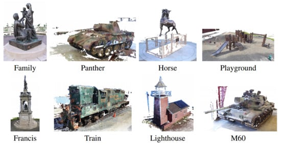
Figure 24.
Results of point clouds from vis-MVSNet [122] on the intermediate set of Tanks and Temples.
4.4. Neural Radiance Fields
4.4.1. Datasets
Mill 19 [151]: This dataset comprises photos of scenes near abandoned industrial parks that were taken directly using UAVs, with a resolution of 4608 × 3456. It contains two main scenes: Mill 19-Building and Mill 19-Rubble (Figure 25). Mill 19-Building consists of 1940 grid photos of an area of 500 × 250 square meters around an industrial building, and Mill 19-Rubble contains 1678 photos of all nearby ruins.
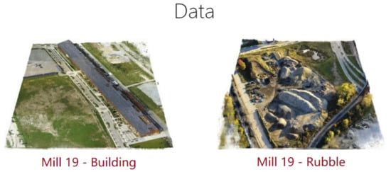
Figure 25.
Examples from the Mill 19 dataset. Ground-truth images of two different scenes called “building” and “rubble” captured by a drone.
4.4.2. Evaluation Metrics
The evaluation metrics for NeRF refer to the image generation task in computer vision, and they include the artificially designed and relatively simple SSIM and PSNR, as well as the LPIPS, which compares the features extracted using a deep learning network. Additionally, some evaluation and visualization results from typical NeRF models are shown in Table 3 and Table 4 and Figure 26, Figure 27 and Figure 28.

Table 3.
Results of different NeRF models on a synthetic NeRF benchmark dataset [129].

Table 4.
Results of different NeRF models on the Mill19 [151] and Quad6K [160] benchmarks.

Figure 26.
Results of Point-NeRF [122] on the Tanks and Temples dataset.
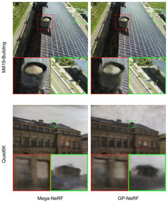
Figure 27.
Visualization results of Mega-NeRF [151] and GP-NeRF [158] on the Mill19 and Quad6K datasets.
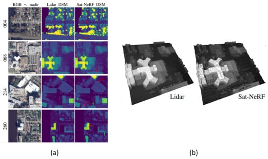
Figure 28.
DSM results of Sat-NeRF [156] on their own dataset: (a) 2D visualization; (b) 3D visualization of scene 608.
SSIM (structure similarity index measure) [172]: This measure quantifies the structural similarity between two images, imitating the human visual system’s perception of structural similarity. It is designed to be sensitive to changes in an image’s local structure. The measure assesses image attributes based on brightness, contrast, and structure. The brightness is estimated using the mean, the contrast is measured using the variance, and the structural similarity is judged using the covariance. The value of the SSIM ranges from 0 to 1. The larger the value, the more similar the two images are. If the value of SSIM is 1, the two images are exactly the same. The formulas are as follows:
- Illumination:
- Contrast:
- Structural Score:
- SSIM:where , , , , respectively, represent the mean and standard deviation of images x and y; is the covariance of images x and y; , , and are constants to prevent division by 0; , , and represent the weights of different features when calculating the similarity.
PSNR (peak signal-to-noise ratio) [148]: The PSNR, which measures the maximum image signal and background noise, is used to evaluate image quality. The larger the value, the less image distortion there is. Generally speaking, a PSNR higher than 40 dB indicates that the image quality is almost as good as that of the original image, a value between 30 and 40 dB usually indicates that the distortion loss of the image quality is within an acceptable range, a value between 20 and 30 dB indicates that the image quality is relatively poor, and a value lower than 20 dB indicates serious image distortion. Given a grayscale image I and a noise image K of size m x n, the MSE (mean square error) is as follows:
where is the maximum pixel value of the image.
LPIPS (learned perceptual image patch similarity): This metric was proposed by Zhang et al. [173] and is also called “perceptual loss”; it is a measurement of the distinction between two images. A generator employs a method capable of reconstructing authentic images from fabricated ones. This is achieved by learning the inverse mapping from generated images to the ground truth. Additionally, it emphasizes the perceptual similarity between these images. The LPIPS fits the situation of human perception better than traditional methods do. A low value of the LPIPS represents high similarity between two images. The specific metric calculates the feature difference between a real sample and a generated sample in a model. This difference is calculated in each channel, and it is the weighted average of all channels. Given the ground-truth image reference block and the noisy image distortion block, the formula for the measure of perceptual similarity is as follows:
where is the weight vector of layer l, ⊙ indicates element-by-element multiplication, and is the image feature.
4.5. Comprehensive Datasets
GL3D (Geometric Learning with 3D Reconstruction [168,169]): This is a large-scale dataset created for 3D reconstruction and geometry-related problems with a total of 125,623 high-resolution images. Most of the images were captured by UAVs at multiple scales and angles, with a large geometric overlap, covering 543 scenes, such as cities, rural areas, and scenic spots (Figure 29). Each scene’s datapoint contains a complete image sequence, geometric labels, and reconstruction results. Besides large scenes, GL3D also includes the reconstruction of small objects to enrich data diversity. For the SfM task, GL3D provides image and camera parameters after de-distortion; for the MVS task, GL3D provides rendering fusion maps and depth maps for different viewpoints based on the Blended MVS dataset.
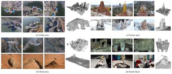
Figure 29.
Examples from the GL3D dataset. Original images of different scenes, including large scenes, small objects, and 3D models of the scenes.
UrbanScene3D [170]: This is a large-scale outdoor dataset for the perception and reconstruction of urban scenes, with a total of more than 128,000 high-resolution images, including 10 virtual scenes and six real scenes (Figure 30). The area is 136 square kilometers, including three large-scale urban scenes covering an area of more than 24 square kilometers and two complete real scenes covering an area of more than one square kilometer. In order to evaluate the reconstruction accuracy and completeness of the reconstructed models of real scenes, UrbanScene3D used LiDAR scanners with GPS positioning equipment to scan entire buildings in the scenes to obtain high-precision scene-scanning point clouds.

Figure 30.
A glance of UrbanScene 3D dataset, with 10 virtual scenes (top) and 6 real scenes (bottom).
5. Results and Discussion
With the advancement of deep learning techniques, passive image-based 3D reconstruction tasks have made significant progress from static indoor scenes to large-scale outdoor environments. However, several challenges still exist.
- Reconstructing areas with texture repetition or weak textures, such as lakes and walls, often leads to reconstruction failures and holes in the reconstructed models. The accuracy of the reconstruction of fine details of objects is still insufficient.
- The construction of datasets for large-scale outdoor scenes is crucial for the development of 3D reconstruction techniques. Currently, there is a scarcity of dedicated datasets for large-scale outdoor scenes, especially city-level real-world scenes.
- The current methods for the 3D reconstruction of large-scale scenes are time-intensive and unable to facilitate real-time reconstruction. Despite the implementation of strategies such as scene partitioning during training and the utilization of computing clusters to expedite the process, these methods still fall short of achieving the efficiency levels required for real-time industrial applications.
- Outdoor scenes contain large numbers of dynamic objects that can significantly impact processes such as image feature matching and camera pose estimation, leading to a decrease in the accuracy of the reconstructed models.
Given the aforementioned challenges and the current state of key technologies in image-based 3D reconstruction, there are several important areas that warrant attention.
- Addressing the issue of regions with weak textures: Previous studies have focused on incorporating semantic information in indoor scenes to recognize and constrain weak-texture areas, thereby improving reconstruction accuracy. However, in the context of the reconstruction of large-scale outdoor scenes, it is crucial to integrate semantic information not only for areas with weak textures but also for common objects in outdoor scenes, such as buildings and dynamic objects. This integration of semantic information represents a significant research direction.
- Building large-scale real-world datasets: Constructing comprehensive datasets for city scenes using data from satellites, aerial planes, drones, and other sources is of paramount importance. Additionally, there is a need for more robust evaluation algorithms for 3D reconstruction. The current metrics, which are largely borrowed from the 2D image domain, may not fully capture the complexities of 3D reconstruction. Future research should focus on developing evaluation algorithms that combine global and local aspects, as well as visual and geometric accuracy, to provide a more comprehensive assessment of 3D reconstruction results.
- Real-time reconstruction: Image-based 3D reconstruction is computationally intensive, making real-time reconstruction a significant challenge. Recent studies have explored methods such as federated learning, where individual drones train using their own data, to improve efficiency. Therefore, integrating techniques such as federated learning and scene partitioning to train lightweight network models using large-scale scene data will be a crucial and challenging research area for achieving the real-time 3D reconstruction of outdoor scenes. This research has significant implications for applications in areas such as smart cities and search-and-rescue missions.
- Fusion of images with other sensors: Another valuable direction is the exploration of efficient fusion techniques that combine images with other sensor data, such as LiDAR data, to address challenges related to some large and complex scenes, including unconventional architecture, vegetation, and occlusions, during the reconstruction of outdoor scenes. By effectively integrating multiple sensor modalities, the accuracy of reconstruction can effectively be improved. This can provide significant enhancements for the planarity of irregular structures and contribute to the restoration of ground points in scenes with dense vegetation.
6. Conclusions
Three-dimensional reconstruction is a fundamental task in the field of computer vision, and its application in outdoor scene reconstruction holds significant importance in real-world scenarios. This study specifically addresses passive methods that are suitable for large-scale outdoor scene reconstruction. A concise overview of both traditional and deep-learning-based approaches to motion recovery, stereo matching, multi-view stereo vision, and Neural Radiance Fields is presented. The development and advancements in each approach are discussed in detail. Furthermore, an introduction to datasets specifically designed for various reconstruction tasks is provided, along with the evaluation metrics commonly employed for assessing the quality of reconstructed scenes. Additionally, in this paper, we discuss the challenges in reconstructing areas with weak or repetitive textures, the scarcity of dedicated datasets for large-scale outdoor scenes, and the need for advanced real-time reconstruction techniques, as well as sensor fusion methods. These challenges, as outlined in Section 5, highlight the crucial areas for future research and development in the field of 3D reconstruction.
Author Contributions
Conceptualization, H.L. and J.Z.; methodology, H.L.; writing—original draft preparation, H.L.; writing—review and editing, J.Z. and X.L.; supervision, J.L.; project administration, L.Z.; funding acquisition, X.L. All authors have read and agreed to the published version of the manuscript.
Funding
This work was supported by the Youth Innovation Promotion Association, CAS (2020132), Science and Disruptive Technology Program, AIRCAS (E3Z207010F) and Rapid Construction and Enhanced Presentation Technology for Three-dimensional Battlefield Environment, AIRCAS (E3M3070106).
Data Availability Statement
No new data were created or analyzed in this study. Data sharing is not applicable to this article.
Conflicts of Interest
The authors declare no conflicts of interest.
References
- Yu, H.; Feng, S.; Cui, L. Research on multi-scale 3D modeling method for urban digital twin. Appl. Electron. Tech. 2022, 48, 78–80+85. [Google Scholar] [CrossRef]
- Martinez Espejo Zaragoza, I.; Caroti, G.; Piemonte, A. The use of image and laser scanner survey archives for cultural heritage 3D modelling and change analysis. ACTA IMEKO 2021, 10, 114–121. [Google Scholar] [CrossRef]
- Liu, Z.; Dai, Z.; Tian, S. Review of non-contact three-dimensional reconstruction techniques. Sci. Technol. Eng. 2022, 22, 9897–9908. [Google Scholar]
- Tachella, J.; Altmann, Y.; Mellado, N.; McCarthy, A.; Tobin, R.; Buller, G.S.; Tourneret, J.Y.; McLaughlin, S. Real-time 3D reconstruction from single-photon lidar data using plug-and-play point cloud denoisers. Nat. Commun. 2019, 10, 4984. [Google Scholar] [CrossRef] [PubMed]
- Wang, J.; Liang, Y. Generation and detection of structured light: A review. Front. Phys. 2021, 9, 688284. [Google Scholar] [CrossRef]
- Liu, B.; Yang, F.; Huang, Y.; Zhang, Y.; Wu, G. Single-Shot Three-Dimensional Reconstruction Using Grid Pattern-Based Structured-Light Vision Method. Appl. Sci. 2022, 12, 10602. [Google Scholar] [CrossRef]
- Wang, C.; Wen, C.; Dai, Y.; Yu, S.; Liu, M. Urban 3D modeling with mobile laser scanning: A review. Virtual Real. Intell. Hardw. 2020, 2, 175–212. [Google Scholar] [CrossRef]
- Rüfenacht, D.; Fredembach, C.; Süsstrunk, S. Automatic and accurate shadow detection using near-infrared information. IEEE Trans. Pattern Anal. Mach. Intell. 2013, 36, 1672–1678. [Google Scholar] [CrossRef] [PubMed]
- Panchal, M.H.; Gamit, N.C. A comprehensive survey on shadow detection techniques. In Proceedings of the 2016 International Conference on Wireless Communications, Signal Processing and Networking (WiSPNET), Chennai, India, 23–25 March 2016; pp. 2249–2253. [Google Scholar]
- Tychola, K.A.; Tsimperidis, I.; Papakostas, G.A. On 3D reconstruction using RGB-D cameras. Digital 2022, 2, 401–421. [Google Scholar] [CrossRef]
- Wadhwa, P.; Thielemans, K.; Efthimiou, N.; Wangerin, K.; Keat, N.; Emond, E.; Deller, T.; Bertolli, O.; Deidda, D.; Delso, G.; et al. PET image reconstruction using physical and mathematical modelling for time of flight PET-MR scanners in the STIR library. Methods 2021, 185, 110–119. [Google Scholar] [CrossRef]
- Woodham, R.J. Photometric method for determining surface orientation from multiple images. Opt. Eng. 1980, 19, 139–144. [Google Scholar] [CrossRef]
- Ju, Y.; Shi, B.; Chen, Y.; Zhou, H.; Dong, J.; Lam, K.M. GR-PSN: Learning to Estimate Surface Normal and Reconstruct Photometric Stereo Images. IEEE Trans. Vis. Comput. Graph. 2023. online ahead of print. [Google Scholar] [CrossRef] [PubMed]
- Yang, Y.; Liu, J.; Ni, Y.; Li, C.; Wang, Z. Accurate normal measurement of non-Lambertian complex surface based on photometric stereo. IEEE Trans. Instrum. Meas. 2023, 72, 5032511. [Google Scholar] [CrossRef]
- Ikehata, S. Scalable, Detailed and Mask-Free Universal Photometric Stereo. In Proceedings of the IEEE/CVF Conference on Computer Vision and Pattern Recognition, Vancouver, BC, Canada, 18–22 June 2023; pp. 13198–13207. [Google Scholar]
- Zheng, T.X.; Huang, S.; Li, Y.F.; Feng, M.C. Key techniques for vision based 3D reconstruction: A review. Acta Autom. Sin. 2020, 46, 631–652. [Google Scholar]
- Jiang, S.; Jiang, C.; Jiang, W. Efficient structure from motion for large-scale UAV images: A review and a comparison of SfM tools. ISPRS J. Photogramm. Remote Sens. 2020, 167, 230–251. [Google Scholar] [CrossRef]
- Snavely, N.; Seitz, S.M.; Szeliski, R. Photo tourism: Exploring photo collections in 3D. ACM ACM Trans. Graph. 2006, 25, 835–846. [Google Scholar] [CrossRef]
- Liang, Y.; Yang, Y.; Fan, X.; Cui, T. Efficient and Accurate Hierarchical SfM Based on Adaptive Track Selection for Large-Scale Oblique Images. Remote Sens. 2023, 15, 1374. [Google Scholar] [CrossRef]
- Ye, Z.; Bao, C.; Zhou, X.; Liu, H.; Bao, H.; Zhang, G. EC-SfM: Efficient Covisibility-based Structure-from-Motion for Both Sequential and Unordered Images. IEEE Trans. Circuits Syst. Video Technol. 2023, 34, 110–123. [Google Scholar] [CrossRef]
- Chen, Y.; Yu, Z.; Song, S.; Yu, T.; Li, J.; Lee, G.H. AdaSfM: From Coarse Global to Fine Incremental Adaptive Structure from Motion. arXiv 2023, arXiv:2301.12135. [Google Scholar]
- Moulon, P.; Monasse, P.; Marlet, R. Adaptive structure from motion with a contrario model estimation. In Proceedings of the Computer Vision–ACCV 2012: 11th Asian Conference on Computer Vision, Daejeon, Republic of Korea, 5–9 November 2012; Revised Selected Papers, Part IV 11. Springer: Berlin/Heidelberg, Germany, 2013; pp. 257–270. [Google Scholar]
- Wu, C. Towards linear-time incremental structure from motion. In Proceedings of the 2013 International Conference on 3D Vision-3DV, Seattle, WA, USA, 29 June–1 July 2013; pp. 127–134. [Google Scholar]
- Schonberger, J.L.; Frahm, J.M. Structure-from-motion revisited. In Proceedings of the IEEE Conference on Computer Vision and Pattern Recognition, Las Vegas, NV, USA, 27–30 June 2016; pp. 4104–4113. [Google Scholar]
- Zhu, S.; Shen, T.; Zhou, L.; Zhang, R.; Fang, T.; Quan, L. Accurate, Scalable and Parallel Structure from Motion. Ph.D. Thesis, Hong Kong University of Science and Technology, Hong Kong, China, 2017. [Google Scholar]
- Qu, Y.; Huang, J.; Zhang, X. Rapid 3D reconstruction for image sequence acquired from UAV camera. Sensors 2018, 18, 225. [Google Scholar] [CrossRef]
- Duan, J. Incremental monocular SFM 3D reconstruction method based on graph optimization. Jiangsu Sci. Technol. Inf. 2019, 36, 37–40. [Google Scholar]
- Liu, B.; Liu, X.; Zhang, H. Linear incremental 3D sparse reconstruction system design. Electron. Opt. Control 2019, 26, 100–104+109. [Google Scholar]
- Cui, H.; Shen, S.; Gao, W.; Liu, H.; Wang, Z. Efficient and robust large-scale structure-from-motion via track selection and camera prioritization. ISPRS J. Photogramm. Remote Sens. 2019, 156, 202–214. [Google Scholar] [CrossRef]
- Sturm, P.; Triggs, B. A factorization based algorithm for multi-image projective structure and motion. In Proceedings of the Computer Vision—ECCV’96: 4th European Conference on Computer Vision, Cambridge, UK, 15–18 April 1996; Proceedings Volume II 4. Springer: London, UK, 1996; pp. 709–720. [Google Scholar]
- Crandall, D.; Owens, A.; Snavely, N.; Huttenlocher, D. Discrete-continuous optimization for large-scale structure from motion. In Proceedings of the CVPR 2011, Colorado Springs, CO, USA, 20–25 June 2011; pp. 3001–3008. [Google Scholar]
- Hartley, R.; Aftab, K.; Trumpf, J. L1 rotation averaging using the Weiszfeld algorithm. In Proceedings of the CVPR 2011, Colorado Springs, CO, USA, 20–25 June 2011; pp. 3041–3048. [Google Scholar]
- Wilson, K.; Snavely, N. Robust global translations with 1dsfm. In Proceedings of the Computer Vision–ECCV 2014: 13th European Conference, Zurich, Switzerland, 6–12 September 2014; Proceedings, Part III 13. Springer: Cham, Switzerland, 2014; pp. 61–75. [Google Scholar]
- Sweeney, C.; Sattler, T.; Hollerer, T.; Turk, M.; Pollefeys, M. Optimizing the viewing graph for structure-from-motion. In Proceedings of the IEEE International Conference on Computer Vision, Santiago, Chile, 7–13 December 2015; pp. 801–809. [Google Scholar]
- Cui, H.; Shen, S.; Gao, W.; Hu, Z. Efficient large-scale structure from motion by fusing auxiliary imaging information. IEEE Trans. Image Process. 2015, 24, 3561–3573. [Google Scholar] [PubMed]
- Zhu, S.; Zhang, R.; Zhou, L.; Shen, T.; Fang, T.; Tan, P.; Quan, L. Very large-scale global sfm by distributed motion averaging. In Proceedings of the IEEE Conference on Computer Vision and Pattern Recognition, Salt Lake City, UT, USA, 18–23 June 2018; pp. 4568–4577. [Google Scholar]
- Pang, Q. Research on Fast 3D Reconstruction Technology of Field Scene Based on UAV Image. Ph.D. Thesis, Hong Kong University of Science and Technology, Hong Kong, China, 2022. [Google Scholar]
- Yu, G.; Liu, X.; Shi, C.; Wang, Z. A robust 3D reconstruction method of UAV images. Bull. Surv. Mapp. 2022, 76–81. [Google Scholar]
- Cui, H.; Gao, X.; Shen, S.; Hu, Z. HSfM: Hybrid structure-from-motion. In Proceedings of the IEEE Conference on Computer Vision and Pattern Recognition, Honolulu, HI, USA, 21–26 July 2017; pp. 1212–1221. [Google Scholar]
- Wang, X.; Xiao, T.; Kasten, Y. A hybrid global structure from motion method for synchronously estimating global rotations and global translations. ISPRS J. Photogramm. Remote Sens. 2021, 174, 35–55. [Google Scholar] [CrossRef]
- Li, D.; Xu, L.; Tang, X.S.; Sun, S.; Cai, X.; Zhang, P. 3D imaging of greenhouse plants with an inexpensive binocular stereo vision system. Remote Sens. 2017, 9, 508. [Google Scholar] [CrossRef]
- Zhang, W.; Liu, B.; Li, H. Characteristic point extracts and the match algorithm based on the binocular vision in three dimensional reconstruction. Remote Sens. 2008, 9, 508. [Google Scholar]
- Nguyen, P.H.; Ahn, C.W. Stereo matching methods for imperfectly rectified stereo images. Symmetry 2019, 11, 570. [Google Scholar]
- Scharstein, D.; Szeliski, R. A taxonomy and evaluation of dense two-frame stereo correspondence algorithms. Int. J. Comput. Vis. 2002, 47, 7–42. [Google Scholar] [CrossRef]
- Hamzah, R.A.; Ibrahim, H.; Hassan, A.H.A. Stereo matching algorithm based on per pixel difference adjustment, iterative guided filter and graph segmentation. J. Vis. Commun. Image Represent. 2017, 42, 145–160. [Google Scholar] [CrossRef]
- Hamzah, R.A.; Ibrahim, H. Literature survey on stereo vision disparity map algorithms. J. Sens. 2016, 2016, 8742920. [Google Scholar] [CrossRef]
- Zheng, G.W.; Jiang, X.H. A fast stereo matching algorithm based on fixed-window. Appl. Mech. Mater. 2013, 411, 1305–1313. [Google Scholar] [CrossRef]
- Yang, C.; Li, Y.; Zhong, W.; Chen, S. Real-time hardware stereo matching using guided image filter. In Proceedings of the 26th Edition on Great Lakes Symposium on VLSI, Boston, MA, USA, 18–20 May 2016; pp. 105–108. [Google Scholar]
- Hirschmüller, H.; Innocent, P.R.; Garibaldi, J. Real-time correlation-based stereo vision with reduced border errors. Int. J. Comput. Vis. 2002, 47, 229–246. [Google Scholar] [CrossRef]
- Yoon, K.J.; Kweon, I.S. Adaptive support-weight approach for correspondence search. IEEE Trans. Pattern Anal. Mach. Intell. 2006, 28, 650–656. [Google Scholar] [CrossRef]
- Wang, Z.F.; Zheng, Z.G. A region based stereo matching algorithm using cooperative optimization. In Proceedings of the 2008 IEEE Conference on Computer Vision and Pattern Recognition, Anchorage, AK, USA, 24–26 June 2008; pp. 1–8. [Google Scholar]
- Liu, X. Research on Stereo Matching Algorithm Based on Binocular Stereo vision. Ph.D. Thesis, Central South University, Changsha, China, 2011. [Google Scholar]
- Zhong, D.; Yao, J.; Guo, T. Stereo Matching Algorithm Based on Image Segmentation. Video Eng. 2014, 38, 5–7+12. [Google Scholar]
- Brown, M.Z.; Burschka, D.; Hager, G.D. Advances in computational stereo. IEEE Trans. Pattern Anal. Mach. Intell. 2003, 25, 993–1008. [Google Scholar] [CrossRef]
- Sung, M.C.; Lee, S.H.; Cho, N.I. Stereo Matching Using Multi-directional Dynamic Programming. In Proceedings of the 2006 International Symposium on Intelligent Signal Processing and Communications, Yonago, Japan, 12–15 December 2006; pp. 697–700. [Google Scholar]
- Li, K.; Wang, S.; Yuan, M.; Chen, N. Scale invariant control points based stereo matching for dynamic programming. In Proceedings of the 2009 9th International Conference on Electronic Measurement & Instruments, Beijing, China, 16–19 August 2009; pp. 3–769. [Google Scholar]
- Hu, T.; Qi, B.; Wu, T.; Xu, X.; He, H. Stereo matching using weighted dynamic programming on a single-direction four-connected tree. Comput. Vis. Image Underst. 2012, 116, 908–921. [Google Scholar] [CrossRef]
- Sun, J.; Zheng, N.N.; Shum, H.Y. Stereo matching using belief propagation. IEEE Trans. Pattern Anal. Mach. Intell. 2003, 25, 787–800. [Google Scholar]
- Zhou, Z.; Fan, J.; Zhao, J.; Liu, X. Parallel stereo matching algorithm base on belief propagation. Opt. Precis. Eng. 2011, 19, 2774–2781. [Google Scholar] [CrossRef]
- Hong, L.; Chen, G. Segment-based stereo matching using graph cuts. In Proceedings of the 2004 IEEE Computer Society Conference on Computer Vision and Pattern Recognition, 2004. CVPR 2004, Washington, DC, USA, 19 July 2004; Volume 1, p. I. [Google Scholar]
- Bleyer, M.; Gelautz, M. Graph-cut-based stereo matching using image segmentation with symmetrical treatment of occlusions. Signal Process. Image Commun. 2007, 22, 127–143. [Google Scholar] [CrossRef]
- Lempitsky, V.; Rother, C.; Blake, A. Logcut-efficient graph cut optimization for markov random fields. In Proceedings of the 2007 IEEE 11th International Conference on Computer Vision, Rio De Janeiro, Brazil, 14–21 October 2007; pp. 1–8. [Google Scholar]
- He, X.; Zhang, G.; Dong, J. Improved stereo matching algorithm based on image segmentation. Microelectron. Comput. 2014, 31, 61–66. [Google Scholar]
- Hirschmuller, H. Stereo processing by semiglobal matching and mutual information. IEEE Trans. Pattern Anal. Mach. Intell. 2007, 30, 328–341. [Google Scholar] [CrossRef] [PubMed]
- Zabih, R.; Woodfill, J. Non-parametric local transforms for computing visual correspondence. In Proceedings of the Computer Vision—ECCV’94: Third European Conference on Computer Vision, Stockholm, Sweden, 2–6 May 1994; Proceedings, Volume II 3. Springer: Berlin/Heidelberg, Germany, 1994; pp. 151–158. [Google Scholar]
- Hermann, S.; Klette, R. Iterative semi-global matching for robust driver assistance systems. In Proceedings of the Asian Conference on Computer Vision, Daejeon, Republic of Korea, 5–9 November 2012; Springer: Berlin/Heidelberg, Germany, 2012; pp. 465–478. [Google Scholar]
- Rothermel, M.; Wenzel, K.; Fritsch, D.; Haala, N. SURE: Photogrammetric surface reconstruction from imagery. In Proceedings of the Proceedings LC3D Workshop, Berlin, Germany, 4–5 December 2012; Volume 8. [Google Scholar]
- Jie, P. 3D Surface Reconstruction and Optimization Based on Geometric and Radiometric Integral Imaging Model. Ph.D. Thesis, Wuhan University, Wuhan, China, 2016. [Google Scholar]
- Li, Y.; Li, Z.; Yang, C.; Zhong, W.; Chen, S. High throughput hardware architecture for accurate semi-global matching. Integration 2019, 65, 417–427. [Google Scholar] [CrossRef]
- Chai, Y.; Yang, F. Semi-global stereo matching algorithm based on minimum spanning tree. In Proceedings of the 2018 2nd IEEE Advanced Information Management, Communicates, Electronic and Automation Control Conference (IMCEC), Xi’an, China, 25–27 May 2018; pp. 2181–2185. [Google Scholar]
- Wang, Y.; Qin, A.; Hao, Q.; Dang, J. Semi-global stereo matching of remote sensing images combined with speeded up robust features. Acta Opt. Sin. 2020, 40, 1628003. [Google Scholar] [CrossRef]
- Shrivastava, S.; Choudhury, Z.; Khandelwal, S.; Purini, S. FPGA accelerator for stereo vision using semi-global matching through dependency relaxation. In Proceedings of the 2020 30th International Conference on Field-Programmable Logic and Applications (FPL), Gothenburg, Sweden, 31 August–4 September 2020; pp. 304–309. [Google Scholar]
- Huang, B.; Hu, L.; Zhang, Y. Improved census stereo matching algorithm based on adaptive weight. Comput. Eng. 2021, 47, 189–196. [Google Scholar]
- Zhao, C.; Li, W.; Zhang, Q. Variant center-symmetric census transform for real-time stereo vision architecture on chip. J. Real-Time Image Process. 2021, 18, 2073–2083. [Google Scholar] [CrossRef]
- Lu, Z.; Wang, J.; Li, Z.; Chen, S.; Wu, F. A resource-efficient pipelined architecture for real-time semi-global stereo matching. IEEE Trans. Circuits Syst. Video Technol. 2021, 32, 660–673. [Google Scholar] [CrossRef]
- Kar, A.; Häne, C.; Malik, J. Learning a multi-view stereo machine. Adv. Neural Inf. Process. Syst. 2017, 30. [Google Scholar]
- Kutulakos, K.N.; Seitz, S.M. A theory of shape by space carving. Int. J. Comput. Vis. 2000, 38, 199–218. [Google Scholar] [CrossRef]
- Lhuillier, M.; Quan, L. A quasi-dense approach to surface reconstruction from uncalibrated images. IEEE Trans. Pattern Anal. Mach. Intell. 2005, 27, 418–433. [Google Scholar] [CrossRef]
- Furukawa, Y.; Ponce, J. Accurate, dense, and robust multiview stereopsis. IEEE Trans. Pattern Anal. Mach. Intell. 2009, 32, 1362–1376. [Google Scholar] [CrossRef]
- Shen, S. Accurate multiple view 3d reconstruction using patch-based stereo for large-scale scenes. IEEE Trans. Image Process. 2013, 22, 1901–1914. [Google Scholar] [CrossRef]
- Bloesch, M.; Czarnowski, J.; Clark, R.; Leutenegger, S.; Davison, A.J. Codeslam—Learning a compact, optimisable representation for dense visual slam. In Proceedings of the IEEE Conference on Computer Vision and Pattern Recognition, Salt Lake City, UT, USA, 18–23 June 2018; pp. 2560–2568. [Google Scholar]
- Xue, Y.; Shi, P.; Jia, F.; Huang, H. 3D reconstruction and automatic leakage defect quantification of metro tunnel based on SfM-Deep learning method. Undergr. Space 2022, 7, 311–323. [Google Scholar] [CrossRef]
- Zhou, T.; Brown, M.; Snavely, N.; Lowe, D.G. Unsupervised learning of depth and ego-motion from video. In Proceedings of the IEEE Conference on Computer Vision and Pattern Recognition, Honolulu, HI, USA, 21–26 July 2017; pp. 1851–1858. [Google Scholar]
- Ummenhofer, B.; Zhou, H.; Uhrig, J.; Mayer, N.; Ilg, E.; Dosovitskiy, A.; Brox, T. Demon: Depth and motion network for learning monocular stereo. In Proceedings of the IEEE Conference on Computer Vision and Pattern Recognition, Honolulu, HI, USA, 21–26 July 2017; pp. 5038–5047. [Google Scholar]
- Wang, C.; Buenaposada, J.M.; Zhu, R.; Lucey, S. Learning depth from monocular videos using direct methods. In Proceedings of the IEEE Conference on Computer Vision and Pattern Recognition, Salt Lake City, UT, USA, 18–23 June 2018; pp. 2022–2030. [Google Scholar]
- Tang, C.; Tan, P. Ba-net: Dense bundle adjustment network. arXiv 2018, arXiv:1806.04807. [Google Scholar]
- Zbontar, J.; LeCun, Y. Computing the stereo matching cost with a convolutional neural network. In Proceedings of the IEEE Conference on Computer Vision and Pattern Recognition, Boston, MA, USA, 7–12 June 2015; pp. 1592–1599. [Google Scholar]
- He, K.; Zhang, X.; Ren, S.; Sun, J. Spatial pyramid pooling in deep convolutional networks for visual recognition. IEEE Trans. Pattern Anal. Mach. Intell. 2015, 37, 1904–1916. [Google Scholar] [CrossRef]
- Bromley, J.; Guyon, I.; LeCun, Y.; Säckinger, E.; Shah, R. Signature verification using a “siamese” time delay neural network. Adv. Neural Inf. Process. Syst. 1993, 6, 737–744. [Google Scholar] [CrossRef]
- Luo, J.; Xu, Y.; Tang, C.; Lv, J. Learning inverse mapping by autoencoder based generative adversarial nets. In Proceedings of the Neural Information Processing: 24th International Conference, ICONIP 2017, Guangzhou, China, 14–18 November 2017; Proceedings, Part II 24. Springer: Beijing, China, 2017; pp. 207–216. [Google Scholar]
- Chang, J.R.; Chen, Y.S. Pyramid stereo matching network. In Proceedings of the IEEE Conference on Computer Vision and Pattern Recognition, Salt Lake City, UT, USA, 18–23 June 2018; pp. 5410–5418. [Google Scholar]
- Li, J.; Wang, P.; Xiong, P.; Cai, T.; Yan, Z.; Yang, L.; Liu, J.; Fan, H.; Liu, S. Practical Stereo Matching via Cascaded Recurrent Network With Adaptive Correlation. In Proceedings of the IEEE/CVF Conference on Computer Vision and Pattern Recognition (CVPR), New Orleans, LA, USA, 18–24 June 2022; pp. 16263–16272. [Google Scholar]
- Xu, G.; Cheng, J.; Guo, P.; Yang, X. Attention Concatenation Volume for Accurate and Efficient Stereo Matching. In Proceedings of the IEEE/CVF Conference on Computer Vision and Pattern Recognition (CVPR), New Orleans, LA, USA, 18–24 June 2022; pp. 12981–12990. [Google Scholar]
- Wang, C.; Wang, X.; Zhang, J.; Zhang, L.; Bai, X.; Ning, X.; Zhou, J.; Hancock, E. Uncertainty estimation for stereo matching based on evidential deep learning. Pattern Recognit. 2022, 124, 108498. [Google Scholar] [CrossRef]
- Zagoruyko, S.; Komodakis, N. Learning to compare image patches via convolutional neural networks. In Proceedings of the IEEE Conference on Computer Vision and Pattern Recognition, Boston, MA, USA, 7–12 June 2015; pp. 4353–4361. [Google Scholar]
- Khamis, S.; Fanello, S.; Rhemann, C.; Kowdle, A.; Valentin, J.; Izadi, S. Stereonet: Guided hierarchical refinement for real-time edge-aware depth prediction. In Proceedings of the European Conference on Computer Vision (ECCV), Munich, Germany, 8–14 September 2018; pp. 573–590. [Google Scholar]
- Pilzer, A.; Xu, D.; Puscas, M.; Ricci, E.; Sebe, N. Unsupervised adversarial depth estimation using cycled generative networks. In Proceedings of the 2018 International Conference on 3D Vision (3DV), Verona, Italy, 5–8 September 2018; pp. 587–595. [Google Scholar]
- Gwn Lore, K.; Reddy, K.; Giering, M.; Bernal, E.A. Generative adversarial networks for depth map estimation from RGB video. In Proceedings of the IEEE Conference on Computer Vision and Pattern Recognition Workshops, Salt Lake City, UT, USA, 18–22 June 2018; pp. 1177–1185. [Google Scholar]
- Matias, L.P.; Sons, M.; Souza, J.R.; Wolf, D.F.; Stiller, C. Veigan: Vectorial inpainting generative adversarial network for depth maps object removal. In Proceedings of the 2019 IEEE Intelligent Vehicles Symposium (IV), Paris, France, 9–12 June 2019; pp. 310–316. [Google Scholar]
- Mayer, N.; Ilg, E.; Hausser, P.; Fischer, P.; Cremers, D.; Dosovitskiy, A.; Brox, T. A large dataset to train convolutional networks for disparity, optical flow, and scene flow estimation. In Proceedings of the IEEE Conference on Computer Vision and Pattern Recognition, Las Vegas, NV, USA, 27–30 June 2016; pp. 4040–4048. [Google Scholar]
- Kendall, A.; Martirosyan, H.; Dasgupta, S.; Henry, P.; Kennedy, R.; Bachrach, A.; Bry, A. End-to-end learning of geometry and context for deep stereo regression. In Proceedings of the IEEE International Conference on Computer Vision, Venice, Italy, 22–29 October 2017; pp. 66–75. [Google Scholar]
- Wang, Y.; Lai, Z.; Huang, G.; Wang, B.H.; Van Der Maaten, L.; Campbell, M.; Weinberger, K.Q. Anytime stereo image depth estimation on mobile devices. In Proceedings of the 2019 International Conference on Robotics and Automation (ICRA), Montreal, QC, Canada, 20–24 May 2019; pp. 5893–5900. [Google Scholar]
- Zhang, F.; Prisacariu, V.; Yang, R.; Torr, P.H. Ga-net: Guided aggregation net for end-to-end stereo matching. In Proceedings of the IEEE/CVF Conference on Computer Vision and Pattern Recognition, Long Beach, CA, USA, 15–20 June 2019; pp. 185–194. [Google Scholar]
- Yao, Y.; Luo, Z.; Li, S.; Fang, T.; Quan, L. Mvsnet: Depth inference for unstructured multi-view stereo. In Proceedings of the European Conference on Computer Vision (ECCV), Munich, Germany, 8–14 September 2018; pp. 767–783. [Google Scholar]
- Yao, Y.; Luo, Z.; Li, S.; Shen, T.; Fang, T.; Quan, L. Recurrent mvsnet for high-resolution multi-view stereo depth inference. In Proceedings of the IEEE/CVF Conference on Computer Vision and Pattern Recognition, Long Beach, CA, USA, 15–20 June 2019; pp. 5525–5534. [Google Scholar]
- Chen, R.; Han, S.; Xu, J.; Su, H. Point-based multi-view stereo network. In Proceedings of the IEEE/CVF International Conference on Computer Vision, Seoul, Republic of Korea, 27 October–2 November 2019; pp. 1538–1547. [Google Scholar]
- Luo, K.; Guan, T.; Ju, L.; Huang, H.; Luo, Y. P-mvsnet: Learning patch-wise matching confidence aggregation for multi-view stereo. In Proceedings of the IEEE/CVF International Conference on Computer Vision, Seoul, Republic of Korea, 27 October–2 November 2019; pp. 10452–10461. [Google Scholar]
- Xue, Y.; Chen, J.; Wan, W.; Huang, Y.; Yu, C.; Li, T.; Bao, J. Mvscrf: Learning multi-view stereo with conditional random fields. In Proceedings of the IEEE/CVF International Conference on Computer Vision, Seoul, Republic of Korea, 27 October–2 November 2019; pp. 4312–4321. [Google Scholar]
- Yi, H.; Wei, Z.; Ding, M.; Zhang, R.; Chen, Y.; Wang, G.; Tai, Y.W. Pyramid multi-view stereo net with self-adaptive view aggregation. In Proceedings of the Computer Vision–ECCV 2020: 16th European Conference, Glasgow, UK, 23–28 August 2020; Proceedings, Part IX 16. Springer: Berlin/Heidelberg, Germany, 2020; pp. 766–782. [Google Scholar]
- Yu, Z.; Gao, S. Fast-mvsnet: Sparse-to-dense multi-view stereo with learned propagation and gauss-newton refinement. In Proceedings of the IEEE/CVF Conference on Computer Vision and Pattern Recognition, Seattle, WA, USA, 13–19 June 2020; pp. 1949–1958. [Google Scholar]
- Gu, X.; Fan, Z.; Zhu, S.; Dai, Z.; Tan, F.; Tan, P. Cascade cost volume for high-resolution multi-view stereo and stereo matching. In Proceedings of the IEEE/CVF Conference on Computer Vision and Pattern Recognition, Seattle, WA, USA, 13–19 June 2020; pp. 2495–2504. [Google Scholar]
- Yang, J.; Mao, W.; Alvarez, J.M.; Liu, M. Cost volume pyramid based depth inference for multi-view stereo. In Proceedings of the IEEE/CVF Conference on Computer Vision and Pattern Recognition, Seattle, WA, USA, 13–19 June 2020; pp. 4877–4886. [Google Scholar]
- Cheng, S.; Xu, Z.; Zhu, S.; Li, Z.; Li, L.E.; Ramamoorthi, R.; Su, H. Deep stereo using adaptive thin volume representation with uncertainty awareness. In Proceedings of the IEEE/CVF Conference on Computer Vision and Pattern Recognition, Seattle, WA, USA, 13–19 June 2020; pp. 2524–2534. [Google Scholar]
- Yan, J.; Wei, Z.; Yi, H.; Ding, M.; Zhang, R.; Chen, Y.; Wang, G.; Tai, Y.W. Dense hybrid recurrent multi-view stereo net with dynamic consistency checking. In Proceedings of the European Conference on Computer Vision, Glasgow, UK, 23–28 August 2020; pp. 674–689. [Google Scholar]
- Liu, J.; Ji, S. A novel recurrent encoder-decoder structure for large-scale multi-view stereo reconstruction from an open aerial dataset. In Proceedings of the IEEE/CVF Conference on Computer Vision and Pattern Recognition, Seattle, WA, USA, 13–19 June 2020; pp. 6050–6059. [Google Scholar]
- Wang, L.; Gong, Y.; Ma, X.; Wang, Q.; Zhou, K.; Chen, L. Is-mvsnet: Importance sampling-based mvsnet. In Proceedings of the European Conference on Computer Vision, Tel Aviv, Israel, 23–27 October 2022; pp. 668–683. [Google Scholar]
- Chang, D.; Božič, A.; Zhang, T.; Yan, Q.; Chen, Y.; Süsstrunk, S.; Nießner, M. RC-MVSNet: Unsupervised multi-view stereo with neural rendering. In Proceedings of the European Conference on Computer Vision, Tel Aviv, Israel, 23–27 October 2022; pp. 665–680. [Google Scholar]
- Liao, J.; Ding, Y.; Shavit, Y.; Huang, D.; Ren, S.; Guo, J.; Feng, W.; Zhang, K. Wt-mvsnet: Window-based transformers for multi-view stereo. Adv. Neural Inf. Process. Syst. 2022, 35, 8564–8576. [Google Scholar]
- Li, Y.; Zhao, Z.; Fan, J.; Li, W. ADR-MVSNet: A cascade network for 3D point cloud reconstruction with pixel occlusion. Pattern Recognit. 2022, 125, 108516. [Google Scholar] [CrossRef]
- Weilharter, R.; Fraundorfer, F. ATLAS-MVSNet: Attention Layers for Feature Extraction and Cost Volume Regularization in Multi-View Stereo. In Proceedings of the 2022 26th International Conference on Pattern Recognition (ICPR), Montreal, QC, Canada, 21–25 August 2022; pp. 3557–3563. [Google Scholar]
- Zhang, S.; Wei, Z.; Xu, W.; Zhang, L.; Wang, Y.; Zhou, X.; Liu, J. DSC-MVSNet: Attention aware cost volume regularization based on depthwise separable convolution for multi-view stereo. Complex Intell. Syst. 2023, 9, 6953–6969. [Google Scholar] [CrossRef]
- Zhang, J.; Li, S.; Luo, Z.; Fang, T.; Yao, Y. Vis-mvsnet: Visibility-aware multi-view stereo network. Int. J. Comput. Vis. 2023, 131, 199–214. [Google Scholar] [CrossRef]
- Yu, D.; Ji, S.; Liu, J.; Wei, S. Automatic 3D building reconstruction from multi-view aerial images with deep learning. ISPRS J. Photogramm. Remote Sens. 2021, 171, 155–170. [Google Scholar] [CrossRef]
- Yu, A.; Guo, W.; Liu, B.; Chen, X.; Wang, X.; Cao, X.; Jiang, B. Attention aware cost volume pyramid based multi-view stereo network for 3d reconstruction. ISPRS J. Photogramm. Remote Sens. 2021, 175, 448–460. [Google Scholar] [CrossRef]
- Gao, J.; Liu, J.; Ji, S. A general deep learning based framework for 3D reconstruction from multi-view stereo satellite images. ISPRS J. Photogramm. Remote Sens. 2023, 195, 446–461. [Google Scholar] [CrossRef]
- Zhang, Y.; Zhu, J.; Lin, L. Multi-View Stereo Representation Revist: Region-Aware MVSNet. In Proceedings of the IEEE/CVF Conference on Computer Vision and Pattern Recognition, Vancouver, BC, Canada, 18–22 June 2023; pp. 17376–17385. [Google Scholar]
- Huang, B.; Yi, H.; Huang, C.; He, Y.; Liu, J.; Liu, X. M3VSNet: Unsupervised multi-metric multi-view stereo network. In Proceedings of the 2021 IEEE International Conference on Image Processing (ICIP), Virtual, 19–22 September 2021; pp. 3163–3167. [Google Scholar]
- Ma, X.; Gong, Y.; Wang, Q.; Huang, J.; Chen, L.; Yu, F. Epp-mvsnet: Epipolar-assembling based depth prediction for multi-view stereo. In Proceedings of the IEEE/CVF International Conference on Computer Vision, Virtual, 11–17 October 2021; pp. 5732–5740. [Google Scholar]
- Mildenhall, B.; Srinivasan, P.P.; Tancik, M.; Barron, J.T.; Ramamoorthi, R.; Ng, R. Nerf: Representing scenes as neural radiance fields for view synthesis. Commun. ACM 2021, 65, 99–106. [Google Scholar] [CrossRef]
- Zhang, K.; Riegler, G.; Snavely, N.; Koltun, V. Nerf++: Analyzing and improving neural radiance fields. arXiv 2020, arXiv:2010.07492. [Google Scholar]
- Rebain, D.; Jiang, W.; Yazdani, S.; Li, K.; Yi, K.M.; Tagliasacchi, A. DeRF: Decomposed Radiance Fields. arXiv 2020, arXiv:2011.12490. [Google Scholar]
- Deng, K.; Liu, A.; Zhu, J.Y.; Ramanan, D. Depth-supervised nerf: Fewer views and faster training for free. In Proceedings of the IEEE/CVF Conference on Computer Vision and Pattern Recognition, New Orleans, LA, USA, 18–24 June 2022; pp. 12882–12891. [Google Scholar]
- Barron, J.T.; Mildenhall, B.; Tancik, M.; Hedman, P.; Martin-Brualla, R.; Srinivasan, P.P. Mip-NeRF: A Multiscale Representation for Anti-Aliasing Neural Radiance Fields. arXiv 2013, arXiv:2103.13415. [Google Scholar]
- Barron, J.T.; Mildenhall, B.; Verbin, D.; Srinivasan, P.P.; Hedman, P. Mip-NeRF 360: Unbounded Anti-Aliased Neural Radiance Fields. In Proceedings of the 2022 IEEE/CVF Conference on Computer Vision and Pattern Recognition (CVPR), New Orleans, LA, USA, 18–24 June 2022. [Google Scholar]
- Chen, X.; Zhang, Q.; Li, X.; Chen, Y.; Ying, F.; Wang, X.; Wang, J. Hallucinated Neural Radiance Fields in the Wild. arXiv 2021, arXiv:2111.15246. [Google Scholar]
- Li, Z.; Wang, Q.; Cole, F.; Tucker, R.; Snavely, N. Dynibar: Neural dynamic image-based rendering. In Proceedings of the IEEE/CVF Conference on Computer Vision and Pattern Recognition, Vancouver, BC, Canada, 18–22 June 2023; pp. 4273–4284. [Google Scholar]
- Yang, G.; Wei, G.; Zhang, Z.; Lu, Y.; Liu, D. MRVM-NeRF: Mask-Based Pretraining for Neural Radiance Fields. arXiv 2023, arXiv:2304.04962. [Google Scholar]
- Chen, A.; Xu, Z.; Zhao, F.; Zhang, X.; Xiang, F.; Yu, J.; Su, H. Mvsnerf: Fast generalizable radiance field reconstruction from multi-view stereo. In Proceedings of the IEEE/CVF International Conference on Computer Vision, Virtual, 11–17 October 2021; pp. 14124–14133. [Google Scholar]
- Xu, Q.; Xu, Z.; Philip, J.; Bi, S.; Shu, Z.; Sunkavalli, K.; Neumann, U. Point-nerf: Point-based neural radiance fields. In Proceedings of the IEEE/CVF Conference on Computer Vision and Pattern Recognition, New Orleans, LA, USA, 18–24 June 2022; pp. 5438–5448. [Google Scholar]
- Guo, H.; Peng, S.; Lin, H.; Wang, Q.; Zhang, G.; Bao, H.; Zhou, X. Neural 3d scene reconstruction with the manhattan-world assumption. In Proceedings of the IEEE/CVF Conference on Computer Vision and Pattern Recognition, New Orleans, LA, USA, 18–24 June 2022; pp. 5511–5520. [Google Scholar]
- Yen-Chen, L.; Florence, P.; Barron, J.T.; Rodriguez, A.; Isola, P.; Lin, T.Y. inerf: Inverting neural radiance fields for pose estimation. In Proceedings of the 2021 IEEE/RSJ International Conference on Intelligent Robots and Systems (IROS), Prague, Czech Republic, 27 September–1 October 2021; pp. 1323–1330. [Google Scholar]
- Lin, C.H.; Ma, W.C.; Torralba, A.; Lucey, S. Barf: Bundle-adjusting neural radiance fields. In Proceedings of the IEEE/CVF International Conference on Computer Vision, Virtual, 11–17 October 2021; pp. 5741–5751. [Google Scholar]
- Martin-Brualla, R.; Radwan, N.; Sajjadi, M.S.; Barron, J.T.; Dosovitskiy, A.; Duckworth, D. Nerf in the wild: Neural radiance fields for unconstrained photo collections. In Proceedings of the IEEE/CVF Conference on Computer Vision and Pattern Recognition, Nashville, TN, USA, 20–25 June 2021; pp. 7210–7219. [Google Scholar]
- Rückert, D.; Franke, L.; Stamminger, M. Adop: Approximate differentiable one-pixel point rendering. ACM Trans. Graph. (ToG) 2022, 41, 1–14. [Google Scholar] [CrossRef]
- Mildenhall, B.; Hedman, P.; Martin-Brualla, R.; Srinivasan, P.P.; Barron, J.T. Nerf in the dark: High dynamic range view synthesis from noisy raw images. In Proceedings of the IEEE/CVF Conference on Computer Vision and Pattern Recognition, New Orleans, LA, USA, 18–24 June 2022; pp. 16190–16199. [Google Scholar]
- Rudnev, V.; Elgharib, M.; Smith, W.; Liu, L.; Golyanik, V.; Theobalt, C. Nerf for outdoor scene relighting. In Proceedings of the European Conference on Computer Vision, Tel Aviv, Israel, 23–27 October 2022; pp. 615–631. [Google Scholar]
- Ost, J.; Mannan, F.; Thuerey, N.; Knodt, J.; Heide, F. Neural scene graphs for dynamic scenes. In Proceedings of the IEEE/CVF Conference on Computer Vision and Pattern Recognition, Nashville, TN, USA, 20–25 June 2021; pp. 2856–2865. [Google Scholar]
- Paul, N. TransNeRF-Improving Neural Radiance Fields Using Transfer Learning for Efficient Scene Reconstruction. Master’s Thesis, University of Twente, Enschede, The Netherlands, 2021. [Google Scholar]
- Rybkin, O.; Zhu, C.; Nagabandi, A.; Daniilidis, K.; Mordatch, I.; Levine, S. Model-based reinforcement learning via latent-space collocation. In Proceedings of the International Conference on Machine Learning, Virtual, 18–24 July 2021; pp. 9190–9201. [Google Scholar]
- Kundu, A.; Genova, K.; Yin, X.; Fathi, A.; Pantofaru, C.; Guibas, L.J.; Tagliasacchi, A.; Dellaert, F.; Funkhouser, T. Panoptic neural fields: A semantic object-aware neural scene representation. In Proceedings of the IEEE/CVF Conference on Computer Vision and Pattern Recognition, New Orleans, LA, USA, 18–24 June 2022; pp. 12871–12881. [Google Scholar]
- Turki, H.; Ramanan, D.; Satyanarayanan, M. Mega-nerf: Scalable construction of large-scale nerfs for virtual fly-throughs. In Proceedings of the IEEE/CVF Conference on Computer Vision and Pattern Recognition, New Orleans, LA, USA, 18–24 June 2022; pp. 12922–12931. [Google Scholar]
- Derksen, D.; Izzo, D. Shadow neural radiance fields for multi-view satellite photogrammetry. In Proceedings of the IEEE/CVF Conference on Computer Vision and Pattern Recognition, Nashville, TN, USA, 20–25 June 2021; pp. 1152–1161. [Google Scholar]
- Xiangli, Y.; Xu, L.; Pan, X.; Zhao, N.; Rao, A.; Theobalt, C.; Dai, B.; Lin, D. Bungeenerf: Progressive neural radiance field for extreme multi-scale scene rendering. In Proceedings of the European Conference on Computer Vision, Tel Aviv, Israel, 23–27 October 2022; pp. 106–122. [Google Scholar]
- Rematas, K.; Liu, A.; Srinivasan, P.P.; Barron, J.T.; Tagliasacchi, A.; Funkhouser, T.; Ferrari, V. Urban radiance fields. In Proceedings of the IEEE/CVF Conference on Computer Vision and Pattern Recognition, New Orleans, LA, USA, 18–24 June 2022; pp. 12932–12942. [Google Scholar]
- Tancik, M.; Casser, V.; Yan, X.; Pradhan, S.; Mildenhall, B.; Srinivasan, P.P.; Barron, J.T.; Kretzschmar, H. Block-nerf: Scalable large scene neural view synthesis. In Proceedings of the IEEE/CVF Conference on Computer Vision and Pattern Recognition, New Orleans, LA, USA, 18–24 June 2022; pp. 8248–8258. [Google Scholar]
- Marí, R.; Facciolo, G.; Ehret, T. Sat-nerf: Learning multi-view satellite photogrammetry with transient objects and shadow modeling using rpc cameras. In Proceedings of the IEEE/CVF Conference on Computer Vision and Pattern Recognition, New Orleans, LA, USA, 18–24 June 2022; pp. 1311–1321. [Google Scholar]
- Huang, J.; Stoter, J.; Peters, R.; Nan, L. City3D: Large-scale urban reconstruction from airborne point clouds. arXiv 2022, arXiv-2201. [Google Scholar]
- Zhang, Y.; Chen, G.; Cui, S. Efficient Large-scale Scene Representation with a Hybrid of High-resolution Grid and Plane Features. arXiv 2023, arXiv:2303.03003. [Google Scholar]
- Xu, L.; Xiangli, Y.; Peng, S.; Pan, X.; Zhao, N.; Theobalt, C.; Dai, B.; Lin, D. Grid-guided Neural Radiance Fields for Large Urban Scenes. In Proceedings of the IEEE/CVF Conference on Computer Vision and Pattern Recognition, Vancouver, BC, Canada, 18–22 June 2023; pp. 8296–8306. [Google Scholar]
- Crandall, D.J.; Owens, A.; Snavely, N.; Huttenlocher, D.P. SfM with MRFs: Discrete-continuous optimization for large-scale structure from motion. IEEE Trans. Pattern Anal. Mach. Intell. 2012, 35, 2841–2853. [Google Scholar] [CrossRef] [PubMed]
- Li, Y.; Snavely, N.; Huttenlocher, D.P. Location recognition using prioritized feature matching. In Proceedings of the Computer Vision–ECCV 2010: 11th European Conference on Computer Vision, Heraklion, Crete, Greece, 5–11 September 2010; Proceedings, Part II 11. Springer: Berlin/Heidelberg, Germany, 2010; pp. 791–804. [Google Scholar]
- Li, S.; He, S.; Jiang, S.; Jiang, W.; Zhang, L. WHU-Stereo: A Challenging Benchmark for Stereo Matching of High-Resolution Satellite Images. IEEE Trans. Geosci. Remote Sens. 2023, 61, 1–14. [Google Scholar] [CrossRef]
- Bosch, M.; Foster, K.; Christie, G.; Wang, S.; Hager, G.D.; Brown, M. Semantic stereo for incidental satellite images. In Proceedings of the 2019 IEEE Winter Conference on Applications of Computer Vision (WACV), Waikoloa Village, HI, USA, 7–11 January 2019; pp. 1524–1532. [Google Scholar]
- Patil, S.; Comandur, B.; Prakash, T.; Kak, A.C. A new stereo benchmarking dataset for satellite images. arXiv 2019, arXiv:1907.04404. [Google Scholar]
- Schops, T.; Schonberger, J.L.; Galliani, S.; Sattler, T.; Schindler, K.; Pollefeys, M.; Geiger, A. A multi-view stereo benchmark with high-resolution images and multi-camera videos. In Proceedings of the IEEE Conference on Computer Vision and Pattern Recognition, Honolulu, HI, USA, 21–26 July 2017; pp. 3260–3269. [Google Scholar]
- Knapitsch, A.; Park, J.; Zhou, Q.Y.; Koltun, V. Tanks and temples: Benchmarking large-scale scene reconstruction. ACM Trans. Graph. (ToG) 2017, 36, 1–13. [Google Scholar] [CrossRef]
- Sensefly. Public Dataset. 2023. Available online: https://www.sensefly.com/education/datasets (accessed on 25 July 2023).
- Yao, Y.; Luo, Z.; Li, S.; Zhang, J.; Ren, Y.; Zhou, L.; Fang, T.; Quan, L. Blendedmvs: A large-scale dataset for generalized multi-view stereo networks. In Proceedings of the IEEE/CVF conference on computer vision and pattern recognition, Seattle, WA, USA, 13–19 June 2020; pp. 1790–1799. [Google Scholar]
- Luo, Z.; Shen, T.; Zhou, L.; Zhu, S.; Zhang, R.; Yao, Y.; Fang, T.; Quan, L. Geodesc: Learning local descriptors by integrating geometry constraints. In Proceedings of the European Conference on Computer Vision (ECCV), Munich, Germany, 8–14 September 2018; pp. 168–183. [Google Scholar]
- Lin, L.; Liu, Y.; Hu, Y.; Yan, X.; Xie, K.; Huang, H. Capturing, reconstructing, and simulating: The urbanscene3d dataset. In Proceedings of the European Conference on Computer Vision, Tel Aviv, Israel, 23–27 October 2022; pp. 93–109. [Google Scholar]
- Aanæs, H.; Jensen, R.R.; Vogiatzis, G.; Tola, E.; Dahl, A.B. Large-scale data for multiple-view stereopsis. Int. J. Comput. Vis. 2016, 120, 153–168. [Google Scholar] [CrossRef]
- Wang, Z.; Bovik, A.C.; Sheikh, H.R.; Simoncelli, E.P. Image quality assessment: From error visibility to structural similarity. IEEE Trans. Image Process. 2004, 13, 600–612. [Google Scholar] [CrossRef]
- Zhang, R.; Isola, P.; Efros, A.A.; Shechtman, E.; Wang, O. The unreasonable effectiveness of deep features as a perceptual metric. In Proceedings of the IEEE conference on Computer Vision and Pattern Recognition, Salt Lake City, UT, USA, 18–23 June 2018; pp. 586–595. [Google Scholar]
Disclaimer/Publisher’s Note: The statements, opinions and data contained in all publications are solely those of the individual author(s) and contributor(s) and not of MDPI and/or the editor(s). MDPI and/or the editor(s) disclaim responsibility for any injury to people or property resulting from any ideas, methods, instructions or products referred to in the content. |
© 2024 by the authors. Licensee MDPI, Basel, Switzerland. This article is an open access article distributed under the terms and conditions of the Creative Commons Attribution (CC BY) license (https://creativecommons.org/licenses/by/4.0/).