Abstract
Food demand is expected to rise significantly by 2050 due to the increase in population; additionally, receding water levels, climate change, and a decrease in the amount of available arable land will threaten food production. To address these challenges and increase food security, input cost reductions and yield optimization can be accomplished using yield precision maps created by machine learning models; however, without considering the spatial structure of the data, the precision map’s accuracy evaluation assessment risks being over-optimistic, which may encourage poor decision making that can lead to negative economic impacts (e.g., lowered crop yields). In fact, most machine learning research involving spatial data, including the unmanned aerial vehicle (UAV) imagery-based yield prediction literature, ignore spatial structure and likely obtain over-optimistic results. The present work is a UAV imagery-based corn yield prediction study that analyzed the effects of image spatial and spectral resolution, image acquisition date, and model evaluation scheme on model performance. We used various spatial generalization evaluation methods, including spatial cross-validation (CV), to (a) identify over-optimistic models that overfit to the spatial structure found inside datasets and (b) estimate true model generalization performance. We compared and ranked the prediction power of 55 vegetation indices (VIs) and five spectral bands over a growing season. We gathered yield data and UAV-based multispectral (MS) and red-green-blue (RGB) imagery from a Canadian smart farm and trained random forest (RF) and linear regression (LR) models using 10-fold CV and spatial CV approaches. We found that imagery from the middle of the growing season produced the best results. RF and LR generally performed best with high and low spatial resolution data, respectively. MS imagery led to generally better performance than RGB imagery. Some of the best-performing VIs were simple ratio index(near-infrared and red-edge), normalized difference red-edge index, and normalized green index. We found that 10-fold CV coupled with spatial CV could be used to identify over-optimistic yield prediction models. When using high spatial resolution MS imagery, RF and LR obtained 0.81 and 0.56 correlation coefficient (CC), respectively, when using 10-fold CV, and obtained 0.39 and 0.41, respectively, when using a k-means-based spatial CV approach. Furthermore, when using only location features, RF and LR obtained an average CC of 1.00 and 0.49, respectively. This suggested that LR had better spatial generalizability than RF, and that RF was likely being over-optimistic and was overfitting to the spatial structure of the data.
1. Introduction
Food demand is expected to rise significantly by 2050 due to an increase in population [1]; additionally, receding water levels, climate change, and a decrease in the amount of available arable land will threaten food production [2]. With access to predictions from a smart farming system (SFS), such as a crop yield prediction system, for example, a farmer could gain insight about the state of the field and could use this information to take corrective action [3] or to plan [4]. Smart farming is a management concept focused on providing the agricultural industry with the infrastructure to leverage Internet of things (IoT) technology, including big data, the cloud, and applied artificial intelligence [5].
A yield prediction system could make early-season yield forecasting, and this would help stakeholders (e.g., farmers, commercial suppliers, governments, and international organizations [6]) by enabling efficient crop management, food security evaluation, food trade planning, and policy design improvements [7].
Furthermore, yield forecasting can increase crop yields and increase environmental sustainability [8]. Early yield predictions can also help crop breeders focus on the more important crop varieties in crop hybrid selection studies [9]. However, high spatial resolution yield datasets are required to train machine learning (ML) models to generate fine-grained yield precision maps.
Fields are heterogeneous by nature [1] despite most farming practices treating the fields as homogeneous. Yield precision maps can be created by deploying an ML model that was trained using local farming data. Sending a tractor into the field frequently can damage the crop. Imagery of a farm can be obtained using remote sensing via satellites, unmanned aerial vehicles (UAVs), aircrafts, or hand-held/tractor-mounted imaging equipment [10] in a non-destructive manner [3]. To obtain imagery using remote sensing, a red-green-blue (RGB) (or visible-light), multispectral (MS), or hyperspectral (HS) camera can be used, where RGB and HS cameras tend to be the most inexpensive and most expensive options, respectively, [11]. Using satellite imagery to enable yield prediction is a common approach [4,12,13,14] and comes with the advantages that (a) there are many free publicly available satellite imagery datasets [15], (b) satellite imagery tends to have high spectral resolution [11], and (c) additional input data or specialized in-field sensing equipment are not required by the farmer [12]; however, satellite-based remote sensing suffers from low spatial and temporal resolutions [16,17,18] (16 days on average for revisits [19]) and is vulnerable to weather [16,18,19]. Performing remote sensing using UAVs is favourable due to the higher spatial and temporal resolutions [20] and the ability to estimate plant height using Structure from Motion (SfM) processing [21]. Plant height data can improve yield prediction models, especially when combined with HS imagery [22]. However, UAV-based approaches that use MS/HS cameras have high monetary costs and high complexity [16], although cost reductions in sensors and UAVs have made UAV-based remote sensing for precision agriculture (PA) more economically feasible [23]. By only using imagery acquired from a UAV for crop analysis, a farmer could avoid deploying many costly sensors in a field [12] and investing in costly yield monitoring equipment [24]. Used frequently in agriculture studies are vegetation indices (VIs). VIs are derived from the reflectance values of the raw imagery by using mathematical operations such as linear combinations or ratios and can be used to represent the state or condition of target vegetation [16]. A common yield prediction approach involves feeding VI features to ML models [25]. Texture indices (TIs), introduced by Haralick et al. [26], can be used to describe local spatial dependence and heterogeneity of an image’s pixels [27]. TIs have been found to improve yield prediction model performance when combined with VIs [27,28] and topographic features [28]; although, compared to VIs, TIs have been used less frequently in the literature [29].
To build a yield prediction system, yield data must first be obtained. During a harvest, a yield monitor will periodically (typically at 1 Hz [30]) record its position (typically accurate to within 1 to 3 m [31]) and the measured yield. Cleaning yield datasets is important before using them for analysis, since they tend to be noisy [30]. Our previous work [32] describes and identifies common yield cleaning steps applied in the literature. Mapping a yield dataset to a grid, the interpolation step, is commonly conducted after cleaning [14,33,34], and is usually performed using kriging and local variograms [35,36], which can be conducted using the Vesper software version 1.6 [14,37]. This step is important, because before performing spatiotemporal analysis on yield and other agriculture datasets, their attributes must be mapped to a common spatial grid, since their attributes are tied to locations and the datasets may have differing spatial resolutions [38]. Once the cleaning and interpolation pre-processing steps have been completed, yield prediction models can be trained. Yield prediction scale can be conducted at global-level [39], region-level/county-level [13,30], field-level/plot-level [7,39], or pixel-level/within-field-level [12,30]. The two most commonly used models for predicting yield are mechanistic crop growth models (MCGMs) (otherwise known as a process-based models or crop simulation models [6]) and data-driven models (e.g., ML) [39]. MCGMs take as input weather, soil, and crop phenology data [12] and simulate the physiological process of crops given input management practices and environmental conditions. They tend to have high complexity, long run times, and complex calibration [6]. Examples of MCGMs include Agricultural Production Systems sIMulator (APSIM) [4], Decision Support System for Agrotechnology Transfer (DSSAT) [4], and Hybrid-Maize [13]. Data-driven models are simpler than MCGMs because they use statistical patterns found in the training data to model the relationship of the input factors affecting yield [39]. Data-driven models also can be used to estimate yield at pixel-level scale [6]. Furthermore, both types of models can be combined using a model-inversion approach [12].
Imagery and phenotyping data tend to be spatially autocorrelated when gathered from a single field [40]. Doing regression or statistical operations on spatially autocorrelated data will lead to overfitting and underestimating prediction errors [41], since datasets that have spatial autocorrelation (SA) violate the data independence assumption made by some ML methodologies [42]. Over-optimistic performance results might be obtained if the datasets are not spatially partitioned [43], and this could lead to incorrect conclusions. An example of such an ML methodology is k-fold cross-validation (KF-CV), which uses random sampling to create the folds [40,43,44]; that is, the chosen sampling technique has an impact on model performance [45,46] and can lead to overfitting if a poor spatial sampling strategy is applied [47]. Instead of applying random sampling, sampling from a specific location can be conducted to create a training dataset, but this may lead to the intra-class imbalance problem, because samples of a class will mostly be similar to each other, leading to poor performance when test samples of that class from different locations are incorrectly classified. This is one of the limitations of spatial cross-validation (CV) [42,48]. After splitting a dataset into training and test sets (used for the final model’s generalizability evaluation), a validation set may also be used for model selection. Model selection occurs when hyperparameters are being tuned and/or the optimal features are being selected, and this is typically conducted by training an ML model using training data and validating the performance using the validation dataset [49], p. 406.Hyperparameter tuning methodologies [43] and feature selection strategies [40] should also take the spatial structure into account. In fact, even though standard/random KF-CV is over-optimistic [44,50], most ML studies in the literature that use earth observation spatial data only apply KF-CV to evaluate their ML models [50], including our previous work [32]. We found that this trend is also observable in the UAV imagery-based yield prediction literature; only one paper (Baghdasaryan et al. [6]) out of the 28 papers related to the present work (see Section 4) clearly performed spatial CV to evaluate model spatial generalizability. Since yield data and imagery from a field will likely be spatially autocorrelated [40], it means the models evaluated in most of these works will likely (a) be over-optimistic [44,50], (b) overfit, and (c) underestimate prediction errors [41]. An over-optimistic model could lead an analyst to draw incorrect conclusions, which could lead to poor economic decisions or other damages. Nevertheless, KF-CV can be appropriate if the model being evaluated is not expected to generalize to new spatial (or temporal, the data’s underlying structures) regions to make new causal inferences. On the other hand, in problems where new unseen spatial regions are expected to be presented to the model (for example, in the context of yield prediction, when a new farmer joins an SFS and uploads field data from an unseen farm) and the ability to perform extrapolation is desired from the model, spatial CV can be used to evaluate the extrapolation performance. Unfortunately, even if spatial CV is designed to avoid underestimating the generalizability error of a model [44], geological trends or environmental gradients may be lost when splitting the training and testing data into spatially disjointed folds [42,46], making the performance evaluation of model extrapolation pessimistic [42] and over-pessimistic if the goal of the learning task is not to extrapolate to new unseen regions [44]. Nevertheless, there are still yield prediction works, which are related to the present work to a lesser degree (those that do not use UAV or aircraft imagery, and do not exclusively use a data-driven model), that did consider (a) the spatial structures of the data and/or evaluated the spatial generalizability of their models [4,7,9,25,51,52,53,54,55,56], and (b) the temporal structures of the data and/or evaluated the temporal generalizability of their models [4,7,14,25,53,55,56,57].
The objectives of the present work are to: (a) bridge the knowledge gap between the UAV imagery-based yield prediction literature and spatial data analysis to reveal and avoid over-optimistic model performance; (b) determine the best time during the growing season (or the best phenological growth stage) to capture imagery to optimize yield prediction results and minimize the number of UAV flight missions; (c) determine the best-performing VIs; (d) determine whether an inexpensive RGB camera can be used instead of a costly MS camera; (e) determine whether the VI calculation step can be skipped in the prediction process by comparing the prediction performance of raw-bands vs. VIs; and (f) determine whether satellite imagery can be used instead of UAV-based imagery to achieve comparable performance at a reduced price. We compared the effectiveness of cameras by examining the difference in yield prediction model performance between: (1) near-infrared (NIR)+RGB band VIs, (2) RGB band VIs, and (3) red-edge-based VIs.
The present work is an extension of a conference paper [32] and improves on the paper by: (a) using imagery from both the RGB and MS camera instead of only using MS camera imagery; (b) considering a larger dataset in the experiments; and (c) evaluating the spatial generalizability of the models by using spatial CV.
The present work is organized as follows:
Section 2 describes the test farm involved in this study and the methodology applied to perform yield prediction using UAV imagery and yield data; Section 3 presents a discussion and analysis of the results; Section 4 discusses the related work and provides a qualitative comparison of various works to the present work; and Section 5 concludes this work and presents future research avenues.
2. Materials and Methods
2.1. Study Site
Corn was grown in the 2021 growing season at a smart farm named Area X.O located in Ottawa, Ontario, Canada (N, W). There were 6 fields (Fields 1, 2, 3, 4, 9, and 11) involved in this study. The size of the fields were 3.38 ac (where 1 ac ≈ 0.405 ha), 4.67 ac, 3.55 ac, 2.07 ac, 1.43 ac, and 48.08 ac, respectively. Figure 1 illustrates a map of the study site.
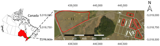
Figure 1.
A map of the test site (Ottawa, ON, Canada). The map illustrates the field numbers and field boundaries and includes a distance scale and coordinate grid that uses the coordinate reference system WGS 84/UTM zone 18N.
2.2. Field Data
2.2.1. Weather
We gathered daily weather data from a local weather station named OTTAWA INTL A that was located near the study site. The dataset was publicly available and was obtained from the Government of Canada’s Weather website, https://climate.weather.gc.ca/historical_data/search_historic_data_e.html, accessed on 23 January 2024. Daily average air temperature and daily total precipitation over the 2021 growing season can be observed in Figures S1 and S2, respectively.
2.2.2. Management
Planting was conducted using a white 6606 planter that had 6 rows (15 ft) 30 inches apart (where 1 ft ≈ 0.3048 m and 1 inch ≈ 2.54 cm). The crops were rainfed. Table 1 presents the tilling techniques, seeding rates, herbicide rates, and fertilizer rates applied to each field, and Table 2 presents the dates of these field activities. The management information presented in this section was obtained from the Trimble platform.

Table 1.
Tillage technique, seeding rates, herbicide application rates, and fertilizer application rates for each field, where CT = conventional tilling (or broadcast), IST = innovative strip-tilling (or fertile stripping), LP = lime pellets, kS/ac = 1000 seeds per acre, 1 lbs ≈ 0.454 kg, 1 gal ≈ 3.785 L, 1 ha ≈ 2.471 ac, and the 7-32-23 notation indicates (7% nitrogen, 32% phosphorus, and 23% potassium) fertilizer.
Table 2.
Field management activity dates.
2.2.3. Imagery
UAV imagery was captured by InDro Robotics from 26 May 2021 to 1 October 2021. The company created orthomosaics using the PIX4Dmapper software version 4.6.4, performed geometric calibration, and performed radiometric calibration. Initially, an Autel EVO 2 drone was used and on 22 June we upgraded to a dual-payload DJI M210 drone. Table 3 provides image acquisition and flight details. The MS camera supported the red (668 nm ± 5 nm), green (560 nm ± 10 nm), blue (475 nm ± 10 nm), NIR (840 nm ± 20 nm), and red-edge (717 nm ± 5 nm) bands [58]. Images were acquired daily from 26 to 31 May and weekly from 8 June to 1 October 2021, generally between 11 a.m. and 3 p.m. The image resolution was between 12.0 and 33.2 megapixels (MP) for the RGB imagery and 1.2 MP for the MS imagery. The image spatial resolution was between 0.7 and 1.3 cm for the RGB imagery and between 2.8 and 3.9 cm for the MS imagery. A Pessl CropVIEW® camera was installed in Field 11 and captured two daily RGB images throughout the season, which were accessible via the Field Climate platform.
Table 3.
UAV image acquisition details over the growing season.
2.2.4. Yield
Shelled corn was harvested on 5 and 6 November 2021, using a John Deere S660 combine equipped with a yield monitor and GPS equipment. Yield readings were sampled at 1 Hz. The harvester had an 8-row combined harvest width of 20 ft that automatically adjusted its width to avoid harvesting previously harvested crop rows. The average moisture content was 22.7%, and the average yield among other descriptive statistics for the raw yield, cleaned yield, and interpolated yield datasets can be found in Tables S1, S2, and S3, respectively, for each field. The harvester’s yield data were calibrated to compensate for the yield sensor lag time delay. Figure S3 provides an example of yield precision map and its corresponding variogram, illustrating that SA exists for a range of approx. 40 m.
2.3. Corn Growth Stage
For the purposes of analyzing the effects of growth stage on crop yield model performance, we assume that all the crops from each field are in the same growth stage, since we only have one CropVIEW camera. Growth stage estimation is important, because it allows the findings of the present work to be compared to other related works that present results in terms of growth stage. Corn growth stages can be split into vegetative (V) and reproductive (R) stages. For example, corn at the V8 vegetative stage has 8 collars, and R1 is the silking reproductive stage [59,60].
2.3.1. Growing Degree Days
In the present work, we estimate the growth stage of the corn by examining the images from the in-field CropVIEW camera, counting the number of plant collars on each plant and using the accumulated growing degree days (GDDs) method [61] (otherwise known as Growing Degree Units (GDUs) [6]). GDDs can be used to estimate crop growth by modelling the number of days that have ideal/sufficient temperature for crop growth [6]. GDD can be calculated as follows [60] in Equation (1):
where is the maximum daily temperature in , is the minimum daily temperature in , and ( = F in this study [6]) is the base temperature for the corresponding crop (corn). Any maximum daily temperature above F is set to 86 (the optimum temperature for corn [62]) and any minimum daily temperature below F is set to 50 in the GDD calculation [62,63,64]. The GDD is accumulated over the season to estimate the growth stage, where a new collar appears approx. every 82 GDD from VE to V10 and every 50 GDD from V11 to Vn [61]. The reproductive development after silking (R1) can also similarly be predicted via GDD accumulation. For stages after R1, we use the accumulated GDD provided in Monsanto [65].
2.3.2. Estimation
By analyzing the CropVIEW imagery, the VE stage started day of year (DoY) 145 (25 May 2021) when the crop emerged. Similar to Oglesby et al. [66], from V1 to V13 we roughly counted the number of collars on each plant from the CropVIEW images. We estimated the VT stage when most of the plants had visible tassels forming in the CropVIEW images. R1 was determined when observable silks were found in the CropVIEW images [66]. From R2 to R6, we used the accumulated GDD suggestions from Monsanto [65], which are approx. 1660, 1859 (interpolated via the days after silking), 1925, 2320, and 2700 accumulated GDD for stages R2, R3, R4, R5, and R6, respectively. This should be a reasonable estimate given that the accumulated GDD for the VT stage Monsanto [65] suggested was 1135, whereas, in the present work, the corn reached the VT stage at DoY 201 with 1195 accumulated GDD (both are relatively similar). Furthermore, Monsanto [65] states that during the R3 stage, the corn ears become brown and dry. We confirmed via the CropVIEW imagery that the ears achieved a peak dry brown colour on DoY 230 with accumulated GDD 1739. This is relatively close to the interpolated 1859 suggested by Monsanto [65], providing further evidence that the growth stage estimates performed in the present work were reasonable. The present work’s growth stage estimates are listed in Table 4.
Table 4.
Estimated corn growth stage [59,60] for 2021 growing season using accumulated GDD [63,65] and in-field crop camera, where DoY = day of year, AGDD = accumulated growing degree days, and GS = growth stage.
2.4. Feature Extraction
Since the yield and imagery datasets did not share the same spatial and temporal resolution, data fusion was required to perform feature extraction.
2.4.1. Yield
We applied most of the yield cleaning steps mentioned in our previous work [32] by implementing the steps in Java version 18.0.1 (the project is open-source and can be found on GitHub https://github.com/patkilleen/geospatial, accessed on 23 January 2024). We did not remove samples from headlands due to small size of the fields. For harvester speed and yield inlier removal, and for turn removal, we applied the forward-backward pass method proposed by Lyle et al. [31]. Note that in our previous work [32] and in the present work, there was a parameter configuration error in the cleaning process, and as a result, the forward-backward pass method was effectively not applied correctly, meaning the yield datasets used in the experiments may have a few more outliers. We used the Vesper software version 1.6 to perform yield semivariogram and interpolation using the block kriging method with a block size 10 m × 10 m, an interpolation grid of 2.5 m × 2.5 m, and a local variogram with 30 lags, 50% lag tolerance, and a maximum distance of 55 m. We removed readings with high kriging variance. We used the R programming language version 4.1.3 sf and sp libraries to remove readings from Field 11 that were inside no-yield areas (e.g., below a power tower). The mean yield (in bu/ac) for each field after cleaning and interpolation is as follows: Field 1 = 107.81, Field 2 = 144.18, Field 3 = 118.18, Field 4 = 77.46, Field 9 = 111.31, and Field 11 = 154.67.
2.4.2. Imagery and Vegetation Indices
In total, 55 VIs were chosen and 5 bands (RGB, NIR, and red-edge) were included as features in the prediction models. A few VIs were defined by the present work using standard VI operations (a ratio or difference, for example) to add additional RGB and red-edge VIs. All the VIs used in this study are listed in the following tables found in Appendix A: NIR+RGB band (NIR-based) VIs in Table A1, RGB band VIs in Table A2, and red-edge-based VIs in Table A3. The RGB imagery had digital pixel values between 0 and 255, so we normalized the values between 0 and 1 and kept both versions because some RGB VIs (e.g., ExG) expect band values between 0 and 1 whereas others (e.g., CIVE) expect band values between 0 and 255.
We used the QGIS software version 3.22.6 to crop the orthomosaics into smaller orthomosaics for each respective field and reduced the resolution of some of the images for computational complexity reasons. We used the R programming language version 4.1.3 raster library to compute VI rasters from the cropped orthomosaics.
2.4.3. Data Fusion
We performed data fusion using the Java program we implemented and applied a mean, maximum, and minimum filter over the imagery data using a circular neighbourhood with a 4.5 m radius around a yield cell’s center, x. We denote this neighbourhood around x as for notation simplicity, where elements in are pixel values (raw-band reflectance or VI). A radius of 4.5 m was chosen to compensate for the fact that the orthomosaics’ extent may be offset by approx. 2 m due to GPS accuracy limitations. Two types of datasets resulted from the fusion, namely a high spatial resolution (HRe) dataset and a low spatial resolution (LRe) dataset. HRe datasets represent the availability of high spatial resolution imagery. Its variables are interpolated yield, mean, max, and min. It captures more fine-grained imagery details by additionally including the maximum and minimum aggregates. LRe datasets represent lower spatial resolution imagery (e.g., satellite imagery). Its variables are interpolated yield and mean. It fails to capture the heterogeneity of fine-grained image details due to the coarse-grained nature of only using the mean aggregation.
2.5. Yield Prediction Experiments
We used the output of the data fusion step to train and evaluate the mono-temporal ML models using various forms of CV. The evaluation metrics used are explained in Section 2.5.1. The models used were random forest (RF) and linear regression (LR). RF and LR models were chosen since RF [14] and LR [67] have commonly been shown to perform well for yield prediction, and they were implemented using Weka version 3.8.5.
There were four types of CV experiments that we ran, namely two standard KF-CV-based experiments (discussed in Section 2.5.3 and Section 2.5.4, respectively) and two spatial CV experiments (discussed in Section 2.5.5), where 10 iterations of each type of CV experiment were performed.
2.5.1. Evaluation Metrics
The three evaluation metrics used to evaluate the ML models in the present work are the root mean squared error (RMSE), the coefficient of determination (), and Pearson’s correlation coefficient (CC), and are defined in Equations (2), (3), and (4), respectively, where is the actual value of sample i, is the predicted value for sample i, n is the number of samples, and and are the mean of the actual and predicted value, respectively.
Root Mean Squared Error
The RMSE describes how much model predictions can be expected to be off by on average, where smaller values indicate better performance. Furthermore, RMSE shares the same units as the target variable [49], pp. 443–444. The values of RMSE lie in the range [68].
Coefficient of Determination
is a measure that compares the model predictions to a baseline model that only predicts the average of the test set [49], pp. 443–447, and it explains how much the target variable can be explained by the predictor variables in terms of variance [49], pp. 443–447 and [68]. values can lie in the range, where larger values mean better performance, is the square of multiple correlation coefficients (CCs), = 0 means the target variable and model predictions are independent, and means the fitted regression line/hyperplane is worse than always predicting the average of the target variable [68].
Correlation Coefficient
The CC (sometimes referred to as R) ranges from −1 to +1 [69], p. 45. It measures the linear association between the target variable and model predictions. The square of the CC can be treated as [70], pp. 432–433, since any negative value can be treated as = 0 by replacing the model with a baseline model that simply predicts the average of the target variable [68].
2.5.2. Model Hyperparameters
Every experiment used the following hyperparameter configuration (Weka’s default):
- RF: bag size = 100%; number of trees = 100; number of attributes/features = 2 for HRe and 1 for LRe; leaf minimum number of instances = 1; minimum variance for a split = 0.001 (i.e., ); unlimited tree depth; number of decimal places = 2; and random number generation seed = 1.
- LR: the M5 attribute/feature selection method was chosen; ridge parameter = ; and number of decimal places = 4.
2.5.3. Location-Only Standard K-Fold Cross-Validation
To explore the extent of the effects SA may have on the yield prediction experiments in the present work, as suggested by Ploton et al. [71], 10-fold CV experiments were conducted using only location features to train field-level models (each model only involved data from a single field) to predict yield for each of the fields.
2.5.4. Standard K-Fold Cross-Validation
In this type of experiment, field-level models were evaluated using 10-fold CV, where folds were created via random sampling, ignoring any spatial structure in the data. Models were trained and evaluated for each of the 6 fields, imagery acquisition dates, VI/raw-band, and both the HRe and LRe dataset types (e.g., for some DoY, datasets would be used to train and evaluate the RF and LR models). We will refer to this type of experiment as a KF-CV experiment.
2.5.5. Spatial Cross-Validation
We apply two types of spatial CV to address the spatial structure in the datasets by strategically creating the folds to reduce SA between the training and testing data.
Leave-One-Field-Out Cross-Validation
In this type of spatial CV experiment, farm-level models were trained and evaluated, and the datasets used were the same as the KF-CV experiments (detailed in Section 2.5.4), but the folds were defined differently by sampling 500 samples from each individual field’s dataset to define a fold. Meaning, instead of 10 folds, 6 folds were created (or 5 folds when a field’s imagery was missing for a day). This sampling scheme was designed to avoid having larger fields’ data be assigned more weight during model training. In this type of experiment, days with imagery available only from a single field were ignored. This type of experiment had two versions, namely leave-one-field-out CV (LOFO-CV) and reverse LOFO-CV (rev-LOFO-CV). LOFO-CV involved training the model using every field but one and testing the model using the remaining field, whereas rev-LOFO-CV involved training the model using only a single field and testing the model using the remaining fields.
K-Means-Based Cross-Validation
This type of experiment, which we refer to as the spatial-k-fold CV (SpKF-CV) experiment, is similar to the LOFO-CV experiments, but here the experiments were field-level and instead of defining a fold as an entire field’s dataset, the folds were defined as samples from clusters resulting from applying the k-means clustering algorithm on location data to create 10 spatially disjoint folds inside a single field. Since the number of samples per cluster varied slightly, the fold sizes were defined using the size of the smallest cluster to make every fold equally sized. This type of experiment had two versions, namely SpKF-CV and reverse SpKF-CV (rev-SpKF-CV). SpKF-CV involved training models using 9 folds and testing the models using the remaining fold, whereas rev-SpKF-CV trained the models with one fold and tested the models using the remaining 9 folds.
3. Results
Figure 2 and Figure 3 illustrate the results of an analysis that involved examining average CC performance of RF and LR over the entire growing season to compare the difference between the evaluation method, RGB and MS imagery, and the image acquisition dates. Two VIs were chosen: ExR (an RGB VI that represents RGB imagery) and (an MS VI that represents MS imagery). These VIs were chosen, since we found was one of the better-performing MS VIs and ExR was one of the better-performing RGB VIs in the present work. The results for each DoY were averaged over both types of datasets (HRe and LRe). Focusing less on the effects of image acquisition date, Figure 4 illustrates the effects that image spatial resolution (HRe vs. LRe) and ML model (RF vs. LR) have on yield prediction performance results for a single image acquisition date (DoY 193). Figure 4 also enables the comparison of RGB imagery vs. MS imagery. ExR was chosen as the VI to represent the RGB imagery, since it was one of the better-performing RGB VIs and it did well for DoY 193. Similarly, was one of the better-performing MS VIs, so it was chosen in this analysis. DoY 193 was chosen, since ExR and did similarly well on that day, which enables analysis of the effects of evaluation method, ML model, and imagery spatial resolution on performance. Figure 5 shows the results of performing yield prediction using KF-CV and using only location data as features.
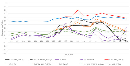
Figure 2.
Random Forest average yield prediction CC performance for 2021 growing season comparing MS imagery () to RGB imagery (ExR), for both LRe and HRe datasets, where KF-CV = k-fold CV, LOFO-CV = leave-one-field-out CV, rev-LOFO-CV = leave-all-but-one-field-out CV, SpKF-CV = spatial k-fold CV, and rev-SpKF-CV = reverse spatial k-fold CV.
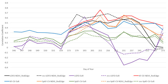
Figure 3.
Linear Regression average yield prediction CC performance for 2021 growing season comparing MS imagery () to RGB imagery (ExR), for both LRe and HRe datasets, where KF-CV = k-fold CV, LOFO-CV = leave-one-field-out CV, rev-LOFO-CV = leave-all-but-one-field-out CV, SpKF-CV = spatial k-fold CV, and rev-SpKF-CV = reverse spatial k-fold CV.
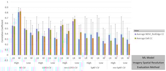
Figure 4.
Evaluation method average yield prediction performance for DoY 193, for MS VI and RGB VI ExR, where the error bars represent 1 standard deviation, KF-CV = k-fold CV, LOFO-CV = leave-one-field-out CV, rev-LOFO-CV = leave-all-but-one-field-out CV, SpKF-CV = spatial k-fold CV, rev-SpKF-CV = reverse spatial k-fold CV, high = HRe dataset, low = LRe dataset, LR = linear regression, and RF = random forest.
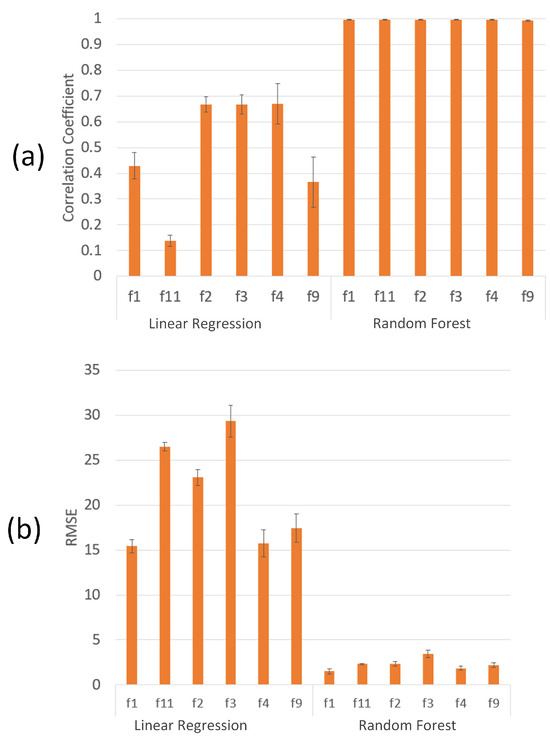
Figure 5.
Location-only features experimental results: 10 iterations of 10-fold CV average yield prediction performance, where the error bars represent 1 standard deviation and fi = Field i. Chart (a) plots CC; chart (b) plots RMSE.
It is worth noting that although we compared the performance results of LOFO-CV and rev-LOFO-CV experiments to the results of the SpKF-CV, rev-SpKF-CV, and KF-CV experiments, strictly speaking, it may not be necessarily correct to compare these results. The SpKF-CV, rev-SpKF-CV, and KF-CV experiments differed in their sampling scheme, but virtually they shared the same input datasets, whereas the LOFO-CV and rev-LOFO-CV experiments’ input datasets were mostly different from those of SpKF-CV, rev-SpKF-CV, and KF-CV. Nevertheless, we compared their results to gather insights on the effects of the sampling scheme on model performance.
3.1. Imagery Type Analysis
3.1.1. Vegetation Index Ranking
In this analysis the VIs were ranked by average performance for each field over different stages in the growing season, ignoring the scale of performance differences between VIs.
In our previous work [32], the CC was used for ranking. In the present work, we chose the measure because (a) it is more adequate for ranking (larger values represent strictly better performance), and (b) large outliers in the RMSE results existed, likely caused by VI divisions by nearly 0, which skewed the RMSE average results. Furthermore, we chose the LOFO-CV and rev-LOFO-CV experiments to avoid having an over-optimistic performance affect rankings. The LR model was chosen since it was the better-performing model for these experiments. Table 5 illustrates the top five best-ranked VIs for each of the defined stages of the growing season, namely, the early, middle (mid), late, and entire season. These seasons were defined as follows: early = {DoY = 173, DoY = 179}, mid = {DoY = 193, DoY = 201, DoY = 211, DoY = 216, DoY = 223, DoY = 231}, late = {DoY = 237, DoY = 245, DoY = 252, DoY = 257, DoY = 273}, and entire = {early ∪ mid ∪ late}. In terms of growth stages, by observing Table 4, early season includes stages V7 and V8 (V10 is not included, for example, since early season includes up to DoY 179 and does not include DoY 186), mid season includes stages from V11 to R3, and late season includes stages R4 and R5. A source of bias is that the mid season contains more growth stages than the early and late seasons.
Table 5.
Five best-performing VIs on average over the growing season by LR model and LOFO-CV and rev-LOFO-CV evaluation methods, where VIs listed in cyan-, orange-, and black-coloured font are NIR-based, red-edge-based, and RGB-based VIs, respectively, LOFO-CV = leave-one-field-out CV, reverse LOFO-CV = leave-all-but-one-field-out CV, HRe = high spatial resolution dataset, LRe = low spatial resolution dataset, and the VIs are defined in Table A1, Table A2 and Table A3 in Appendix A.
The RGB VIs included in this analysis were only from imagery gathered by the RGB camera and the MS VIs were from the MS camera. Note that the early season only included two acquisition dates because no MS imagery was gathered before that.
By analyzing Table 5 we can see that
- In general, MS imagery leads to better performance than RGB imagery. We can see two RGB VIs that were among the top five best-ranked VIs: in early season for LOFO-CV-LRe and IKAW4 in the late season for rev-LOFO-CV-HRe.
- For rev-LOFO-CV, we can see that red-edge-based VIs do better from middle to late season.
- NIR-based VIs do especially well earlier in the season, which makes sense, since the NIR reflectance decreases around the middle of the growing season [18]. NDVI is also among the top-ranked VIs in early season.
- Another noteworthy VI is the , which is relatively high ranking for the LOFO-CV experiments using HRe data.
- We can also see that the red-edge raw-band is frequently among the top five highest-ranked VIs, suggesting we could save computational costs and skip the VI calculation step by using the red-edge band directly.
- Over the entire growing season, the three VIs among the top five best ranking performance for each of HRe, LRe, LOFO-CV, and rev-LOFO-CV, are , , and NG.
Among the five worst-performing VIs for HRe, LRe, LOFO-CV, and rev-LOFO-CV, which can be found in Table 6, the following observations can be made:
Table 6.
Five worst-performing VIs on average over the growing season by LR model and LOFO-CV and rev-LOFO-CV evaluation methods, where VIs listed in cyan-, orange-, and black-coloured font are NIR-based, red-edge-based, and RGB-based VIs, respectively, LOFO-CV = leave-one-field-out CV, reverse LOFO-CV = leave-all-but-one-field-out CV, HRe = high spatial resolution dataset, LRe = low spatial resolution dataset, and the VIs are defined in Table A1, Table A2 and Table A3 in Appendix A.
- Approximately 70% of these VIs included the blue band in their definition, whereas the top five best-ranked VIs rarely included the blue band in their definition. In fact, the middle of the season had no blue-based VIs that were ranked among the top five. Interestingly, was ranked among the top five best VIs for LOFO-CV-HRe, suggesting the blue band still has prediction power when combined with other MS bands.
- Approximately 30% of the raw-bands, all of which were RGB, were among the worst-performing VIs.
- Nearly all the worst-performing VIs (95%) were RGB-based. There were no NIR-based VIs in the early and middle seasons among the five worst VIs. Only in late season for rev-LOFO-LRe were there two NIR-based VIs among the worst VIs. On the other hand, for red-edge-based VIs, there were no red-edge-based VIs among the worst during late season. Only in the early and middle seasons for LOFO-CV-HRe was there a red-edge-based VI among the five worst.
3.1.2. MS Imagery vs. RGB Imagery
We can see in Figure 6 that in the over-optimistic case when using KF-CV, on average MS consistently outperforms RGB imagery for both LR and RF and for both HRe and LRe datasets.
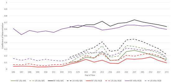
Figure 6.
KF-CV average coefficient of determination () over the growing season for all fields and VIs, where RF = random forest, LR = linear regression, 10F-CV = 10-fold CV, MS = multispectral imagery, RGB = red-green-blue imagery, LRe = low spatial resolution dataset, and HRe = high spatial resolution dataset.
We can see in Figure 2 and Figure 3 that for DoY 193, LR-rev-LOFO-ExR (an over-pessimistic evaluation method) does better than (an over-optimistic evaluation method), suggesting RGB imagery can outperform MS imagery. Keep in mind that the performance trends in Figure 2 and Figure 3 are averaged out over both the HRe and LRe dataset types, meaning performance trends such as the excellent results of RF-KF-CV-HRe are masked in this chart. Furthermore, rev-LOFO-ExR also outperforms every othen RGB camera could be used to obtain reasonable results in early-to-mid season, instead of using an expensive MS camera. For almost every other DoY other than 193, the experimental results consistently did better than the ExR. For LR, even the four more pessimistic spatial CV techniques for (rev-LOFO-CV, LOFO-CV, rev-SpKF-CV, and SpKF-CV) outperformed the over-optimistic KF-CV-ExR on multiple occasions during the middle of the season. This was not observable for RF performance, although RF overfitting to the spatial structures of the data may explain these trends. Nevertheless, this suggests MS imagery is generally better for yield prediction than RGB imagery, which is consistent with the findings in other literature [29].
We can see in Figure 4 that in general, led to more standard deviation in the CC performance compared to ExR, except for the SpKF-CV approach. We can also see that for the LOFO-CV experiments (and most other types of experiments), outperforms ExR in average CC performance, whereas for the rev-LOFO-CV experiments, the opposite is the case, ExR outperforms . The rev-LOFO-CV experiments were designed to be more pessimistic than LOFO-CV and act as a baseline to evaluate the true generalizability of a model that is attempting to perform extrapolation from one field’s imagery to a new field’s unseen imagery. In other words, this type of experiment simulates the situation where a cold-start SFS is being deployed, and only data from one farm are available. These results suggest that ExR generalizes better than in a cold-start situation where limited field imagery is available (for DoY 193). This begs the question: for MS imagery, is there a VI that has better average performance for rev-LOFO-CV experiments than ? If such a VI exists, it would suggest that such a VI is better at generalizing when limited field data are available than , meaning the choice of VI could be made based on the amount of data available.
Source of bias: Note that for DoY 193, there was an issue with the NIR band for Field 11, so no MS imagery for Field 11 was considered, whereas there was RGB imagery for Field 11. In addition, the SpKF-CV results using Field 11 data had better performance than the two smallest fields (Fields 4 and 9). This suggests that the LOFO and rev-LOFO results for DoY 193 might have a bias that favours RGB imagery results due to MS imagery missing for Field 11 that same day. Furthermore, some days only had imagery from one field (DoY 211 for both RGB imagery and MS imagery and 231 for MS imagery), so the LOFO-CV and rev-LOFO-CV evaluation methods could not be applied, meaning the data had to be interpolated in Figure 2 and Figure 3 for plot-line continuity. Similar line continuity interpolation for DoY 252 was performed for MS imagery plotted in Figure 6. Furthermore, for DoY 252, we only had RGB imagery available, so the MS performance trends were also interpolated for that day. In particular, if we observe Figure 2 and Figure 3, for DoY 211 and 231 there are spikes in performance, which may be attributed to only having imagery from a single field (Field 3 for DoY 211 and Field 11 for DoY 231 for the MS imagery). This could also be attributed to a previously discussed observation that red-edge-based VIs perform better during the middle to late season in general.
Takeaway: MS imagery, especially imagery containing the red-edge band, obtains the best yield prediction results and should be favoured over RGB imagery if it is available. One could save computational costs and skip the VI calculation step by using the red-edge band directly. The , , and NG VIs were found to be among the VIs with the best yield prediction power for the entire season.
3.2. Effects of Spatial Autocorrelation on Performance
The effects of SA on yield prediction ML model performance are examined in this section by analyzing the results of the location-only feature CV experiments. We can see in Figure 5 that the RF model learns each field’s spatial patterns well, performing virtually perfectly, whereas LR does more poorly and has trouble doing well on every field.
RF obtained 0.996 CC and 2.281 RMSE, on average, and LR obtained 0.490 CC and 21.260 RMSE, on average. Furthermore, Figure 6 compares the results of KF-CV experiments for LR vs. RF, HRe vs. LRe, and MS imagery (the average overall NIR-based and red-edge-based VIs) vs. RGB imagery (the average overall RGB-based VIs from the RGB camera); we can see that the yield prediction performance results obtained from RF when using HRe datasets were quite good even early in the season when images mostly contained soil with little vegetation. Intuitively, good yield prediction performance should be difficult in this situation. Another explanation could be that RF is sensitive to the number of features in the dataset (which we discuss briefly in Section 3.4) and does better with an increased number of features, although, Figure 4 does not support this as the only explanation, since only when HRe and KF-CV are combined does RF do quite well. In all the other spatial CV cases with HRe, RF does not do as well. These observations suggest that the results of applying KF-CV to RF with HRe (RF-KF-CV-HRe) are over-optimistic and are due to RF overfitting to the spatial structure found in HRe datasets instead of learning the reflectance trends in relation to yield.
Takeaway: These results illustrate that one has to be careful with how one designs ML experiments and sampling schemes using crop imagery and yield data, since assuming independence between the training and testing datasets should be avoided when a spatial dependence structure exists; otherwise over-optimistic results may be obtained and this could lead to misinformed decision making by stakeholders.
3.3. ML Model Comparison
We analyze the differences in performance between RF and LR in this section. We can see in Figure 4 and Figure 6 that RF overfits to the spatial structure when RF-KF-CV-HRe is used, since in no other spatial CV method did RF outperform RF-KF-CV-HRe.
The observations we made about RF may be explained by using the location-only feature experiment findings discussed in Section 3.2; that is, RF can make use of the underlying spatial structure in the data to make yield predictions using the HRe dataset type instead of learning reflectance trends, since the HRe dataset by design contains more spatial structure information than LRe. When using LRe datasets, RF appears to overfit less to the spatial structure, since (a) RF’s performance is lower than LR’s for the entire season (shown in Figure 6), and (b) in both the RF-rev-LOFO-CV-LRe and RF-rev-LOFO-CV-HRe experiments ExR did better than RF-KF-CV-LRe (shown in Figure 4).
In general, LR appears to be better at generalizing, which is consistent with claims made by Zhang et al. [67], since (a) over the entire season for KF-CV experiments, the difference in performance of LR for the LRe and HRe datasets is not visibly significant (shown in Figure 6), although it is worth pointing out that HRe generally does lead to slightly better performance over LRe, and (b) the over-optimistic KF-CV results are similar to the over-pessimistic spatial CV results. In fact, LR did generally better than the over-optimistic KF-CV when using LOFO-CV and rev-LOFO-CV, providing further evidence that LR generalizes better than RF when the dataset has a spatial structure (shown in Figure 4).
Furthermore, we can see in Figure 4 that in general, RF tends to have less standard deviation than LR when using ExR (except in the case of rev-LOFO-CV), suggesting that RF produces more consistent prediction results than LR for RGB imagery for DoY 193.
Moreover, by observing Table 7, we found that for rev-LOFO-CV, LRe datasets, and MS imagery, LR does much better than RF, especially at the start of the season. As the season progresses, the performance difference between RF and LR generally decreases. For RGB imagery, the performance difference between LR and RF is larger than MS imagery at the end of the season.
Table 7.
Average performance of LR and RF over the entire season for the LRe datasets and rev-LOFO-CV evaluation method, and for MS imagery (NIR-based and red-edge-based VIs) and RGB imagery, where RGB = red-green-blue, MS = multispectral, RF = random forest, LR = linear regression, and DoY = day of year.
Takeaway: LR has better generalizability than RF when used on yield data with spatial structure, suggesting that complex models may also overfit to spatial structure in datasets if the spatial dependence is not addressed via spatial CV. LR also generally does better than RF with LRe datasets, suggesting LR should be chosen over RF when only satellite imagery is available.
3.4. High vs. Low Spatial Resolution Imagery Analysis
We examine the performance differences between the HRe vs. LRe datasets in this section by examining the performance of the various evaluation methods for DoY 193 (one of the acquisition dates that lead to the best performance for RGB imagery), and and ExR. We can see in Figure 4 that changes in the imagery’s spatial resolution have the most impact on RF. RF does better with HRe than with LRe (especially for KF-CV), suggesting that the good performance of RF-KF-CV-HRe may not exclusively be the result of overfitting to spatial structure; RF may also be taking advantage of the higher resolution imagery and the additional features. LR appears to do slightly better on average with LRe data, except in the case of KF-CV. In particular, the configuration that achieved the best results for DoY 193 using LR involved the LRe data for the rev-LOFO-CV method, suggesting cheaper satellite imagery could be used instead of more expensive UAV imagery.
Takeaway: High spatial resolution imagery obtained from expensive UAV missions is not necessarily required to obtain reasonable results. The less expensive approach of using RGB or MS imagery obtained from a satellite instead of a UAV can be applied to obtain reasonable results if a proper VI is chosen and the image acquisition is well-timed.
3.5. Evaluation Method Comparison
In this section, the performance difference between standard KF-CV and the spatial CV evaluation methods is examined. We can see in Figure 4 that RF generally overfits, whereas LR is better at generalizing. In fact, for two of the pessimistic evaluation techniques, LOFO-CV and rev-LOFO-CV, LR does comparably well compared to the over-optimistic KF-CV method. This is particularly the case for LRe datasets, where both LOFO-CV and rev-LOFO-CV outperform KF-CV. However, the higher LR-LOFO-CV and LR-rev-LOFO-CV performance compared to LR-KF-CV could be attributed to the increased number of training samples per fold compared to the fold size of KF-CV for the smaller fields, since in all cases, both versions of the LR-SpKF-CV did worse than LR-KF-CV, and in these experiments the dataset sizes were similar. This begs the question: to what extent does fold size affect performance?
3.5.1. LOFO-CV vs. rev-LOFO-CV
- We can see that for the RGB VI (ExR) for LOFO-CV and rev-LOFO-CV in Figure 2 and Figure 3, earlier in the season there is no large distinction between both evaluation methods other than the peak performance achieved for DoY 193 by rev-LOFO-CV, although, LOFO-CV does generally better than rev-LOFO-CV later in the season. An observable difference between LR and RF is that negative CC performance is achieved by LR-LOFO-CV later in the season, whereas RF has positive CC performance.
- For both the and ExR, the peak performance achieved is by rev-LOFO-CV.
- There is also some bias that could be introduced in the two types of LOFO-CV experiments, since imagery missions were occasionally conducted 1 to 3 days apart (delayed) from the other fields for some weeks, especially at the end of the season. In fact, LOFO-CV and rev-LOFO-CV do most poorly at the end of the season for both ExR and , which may be attributed to these delays in field imagery acquisition missions.
- There are also days when one field was missing, meaning the two LOFO CV methods (rev-LOFO-CV and LOFO-CV) may have a bias in the results involving experiments with missing fields due to the reduced number of folds.
3.5.2. LOFO-CV vs. SpKF-CV
When observing the LOFO-CV and SpKF-CV (the k-means-based spatial CV) methods for ExR, we can see that earlier in the season there is no large difference between the two; that is, LOFO-CV, rev-LOFO-CV, SpKF-CV, and rev-SpKF-CV are relatively similar in early season (although SpKF-CV does do slightly better). For both ExR and , in the middle of the season, LOFO-CV and rev-LOFO-CV generally do slightly better than SpKF-CV and rev-SpKF-CV, and late in the season, LOFO-CV and rev-LOFO-CV do generally worse than the SpKF-CV and rev-SpKF-CV approaches (especially for ExR), further suggesting these delays in field imagery acquisition missions negatively impacted the LOFO-CV and rev-LOFO-CV performance. Since LOFO-CV is a farm-level evaluation method and the SpKF-CV is a field-level evaluation method, another possible reason for LOFO-CV doing better than SpKF-CV earlier in the season and doing more poorly than SpKF-CV later in the season is that the early-to-middle and middle-to-late season, for ExR and , respectively, hold spectral information patterns that are strongly tied to potential yield and are present in each of the fields’ imagery, whereas later in the season these yield-reflectance relationships weaken and become field-dependent (e.g., depending on the management practices applied to the field) and have trouble being used by models to be generalized to each field. Note that the comparison between LOFO-CV and SpKF-CV is not necessarily fair because the fold sizes are not the same. SpKF-CV is more pessimistic because of the smaller fold sizes.
The two types of SpKF-CV methods have more standard deviation than LOFO-CV and rev-LOFO-CV, probably due to the smaller training dataset size.
3.5.3. SpKF-CV vs. rev-SpKF-CV
From Figure 2 and Figure 3, we can see that, for ExR and , SpKF-CV generally does better than rev-SpKF-CV for the entire season, except for DoY 211 (and DoY 257 for LR) for . This suggests increasing the amount of available training data from a field will increase model performance.
Table 8 presents the combined average performance results of LR and RF for the two types of SpKF-CV experiments for each field. We can see that generally, Field 11 imagery led to better performance. This might be because the spatially wide clusters in Field 11 were wide enough to capture the underlying imagery yield trends, whereas the smaller fields did not have wide enough clusters to do the same. For SpKF-CV experiments, imagery of Fields 2 and 4 had the worst performance, which may be due to a lack of yield spatial variability (clusters of low yield areas were mostly found in a single sub-region of the fields instead of multiple sub-regions). For rev-SpKF-CV experiments, Field 9 imagery had the worst performance, probably because Field 9 was the smallest field.
Table 8.
Combined average LR and RF performance of each field over the entire season for SpKF-CV and rev-SpKF-CV, HRe and LRe, and for MS imagery (NIR-based and red-edge-based VIs) and RGB imagery, where SpKF-CV = spatial k-fold CV, rev-SpKF-CV = reverse spatial k-fold CV, LRe = low spatial resolution dataset, HRe = high spatial resolution dataset, RGB = red-green-blue, and MS = multispectral.
Takeaway: Results suggest that LOFO-CV and rev-LOFO-CV have the advantage of evaluating the extrapolation ability of a model when sampling regions (different fields) are relatively similar, but when the sampling regions start to differ (field imagery that do not share the same acquisition date) these two methods become overly pessimistic and the SpKF-CV should be favoured since the imagery from a single field was typically always taken on the same day (in rare circumstance a field mission may have been split into two consecutive days due to drone battery issues). However, the SpKF-CV struggles due to having lower training dataset sizes compared to LOFO-CV, especially for the smaller fields, and as a result, is also over-pessimistic. Therefore, the SpKF-CV may be appropriate when field sizes are sufficiently large, whereas LOFO-CV would be more appropriate when imagery from multiple smaller fields is available. Using KF-CV alone as an evaluation method is not sufficient to fairly assess the generalizability and extrapolation ability of a model; spatial CV and location-only feature CV evaluation methods should also be used. One should keep in mind that there is bias in the assessment of the extrapolation ability of the models used in the present work using any of the spatial CV methods since the fields are all from the same farm and share the same weather conditions.
3.6. Imagery Acquisition Date Analysis
We can see in Figure 2 and Figure 3 that the middle of the season is generally the best time to capture imagery for maximizing yield prediction performance results, whereas early season led to poor performance and late season had generally lower performance.
Takeaway: The middle of the season is the best time to acquire imagery to maximize yield prediction results.
3.7. Data Processing Time Analysis
An execution time analysis of the image processing and ML models tested in the present work was performed and is explained in this section to illustrate the feasibility of deploying the applied methodology to a live setting. Table 9 presents the average execution times for the image pre-processing steps. Table 10 shows the average execution times to create all the ML input datasets for a single DoY. Table 11 shows the average execution times of the ML experiments.
Table 9.
Average (sampled over three random acquisition dates) image processing steps execution time, where VI = vegetation index, RGB = red-green-blue imagery, MS = multispectral imagery, smaller fields = Fields 1 to 9, min = minute, and h = hours.
Table 10.
Average (sampled over three random acquisition dates) execution time to split and create all datasets for all VIs and fields, where KF-CV = k-fold CV, LOFO-CV = leave-one-field-out CV, rev-LOFO-CV = leave-all-but-one-field-out CV, SpKF-CV = spatial k-fold CV, rev-SpKF-CV = reverse spatial k-fold CV, RGB = red-green-blue imagery, MS = multispectral imagery, and min = minute.
Table 11.
Average (sampled over three random acquisition dates and five random VIs) execution times for ML experiments, where KF-CV = k-fold CV, LOFO-CV = leave-one-field-out CV, rev-LOFO-CV = leave-all-but-one-field-out CV, SpKF-CV = spatial k-fold CV, rev-SpKF-CV = reverse spatial k-fold CV, location-only = only location features used, LRe = low spatial resolution dataset, HRe = high spatial resolution dataset, LR = linear regression, RF = random forest, s = second, and m = minute.
3.7.1. Imagery Acquisition
During an image capture mission, the UAV captured MS images (five images, one for each band) and RGB images (a single image) approx. every 1 s and 2 s, respectively. On average, 114.14 Mbps of raw imagery was created during a mission. The average UAV flight duration was 474.6 s (7.9 min) for the smaller fields and 1855.5 s (30.9 min) for Field 11.
3.7.2. Imagery and Yield Pre-Processing
From the imagery stored on the UAV’s SD card, InDro Robotics generated orthomosaics using PIX4D on a machine with the following specifications: 64-bit Windows 10 machine, 64 GB of RAM, a 24-core AMD Ryzen Threadripper 3960X CPU @ 3.8 GHz, and an NVIDIA GeForce RTX 3080 Ti GPU. For a single UAV mission:
- For RGB imagery, six orthomosaics were typically created (one for each field). Sometimes, Field 11 was split into two orthomosaics for a single UAV mission (this was conducted for five missions from August onward), so the orthomosaic with the most imagery and the least amount of noise was chosen for further processing for that DoY. On average, it took 2.4 and 3.1 h to generate orthomosaics for the smaller fields and Field 11, respectively.
- For MS imagery, twelve () orthomosaics were typically created, one for each band and one for NDVI, and two sets of six orthomosaics (one set for Field 11 and another set for the smaller fields) were generated. On average (ignoring a 74.2 h outlier), it took 6.8 and 4.8 h to generate the six single-band orthomosaics for the smaller fields and Field 11, respectively.
The orthomosaic creation process also included 3D surface model creation and a PIX4D output report. After being delivered via an external hard disk drive (HDD) at the end of the 2021 growing season, the orthomosaics were then processed using a machine with the following specifications: a 64-bit Windows 10 desktop, 32 GB of RAM, an 8-core Intel Core i7 CPU @ 3.50 GHz, and a 1 TB solid-state drive (SSD). For the execution time analysis discussed next in this section, three DoYs were randomly sampled for MS imagery and another three DoYs were randomly sampled for RGB imagery; the execution times were approximated by taking the average execution time over those samples. Table 9 shows these results, where the smaller field execution time is the average over the smaller fields. The cropping of the orthomosaics was conducted using QGIS, where fields were cropped into multiple overlapping tiles to avoid reading entire orthomosaics into memory (this was especially problematic with Field 11). Fields 1, 2, 3, 4, 9, and 11 were horizontally partitioned into 5, 6, 4, 6, 5, and 21 tiles, respectively. Some RGB orthomosaics were too big for further processing, so their spatial resolution was lowered to 1.149 cm. The cropped orthomosaic tiles were then processed by the R programming language version 4.1.3 to create VI rasters for each tile. The Rcpp package version 1.0.9 was used to enable the use of C++ to calculate VI rasters in a memory-efficient manner.
The data fusion of the imagery and yield was conducted using Java version 18.0.1, where the cropped orthomosaic tiles were progressively read to fuse each yield sample to its corresponding pixel neighbourhood, where pixels outside field boundaries were ignored. Once fused, the resulting dataset contained every feature and had to be split into smaller HRe and LRe single-VI feature datasets for each fold and for each iteration of the CV experiments using a combination of Java and R programming languages. The average total execution time for all VIs for each evaluation method type (averaged over both HRe and LRe) of this final dataset-splitting step before feeding the datasets to the ML models can be found in Table 10. For the location-only CV, there was no dataset splitting required: we just used the interpolated yield dataset and fed it to Weka.
Takeaway: For orthomosaic generation, on average, orthomosaics with the largest area (greatest number of input images to be stitched together) took the longest execution time. For VI creation and data fusion, Field 11 took the longest execution time compared to the smaller fields. For splitting the datasets, the HRe datasets generally took longer than LRe, probably because HRe had two additional features. The MS imagery took longer than the RGB imagery when splitting the data. This may be explained by the fact that the MS imagery was generally less noisy than the RGB imagery, meaning more samples were found in the MS datasets. The dataset splitting involving clustering took the longest, which was likely due to the added computational complexity of the clustering step.
3.7.3. Machine Learning
For the execution time analysis discussed in this section, three DoYs were randomly sampled for MS imagery and another three DoYs were randomly sampled for RGB imagery, and the execution times were approximated by taking the average execution time over those samples. In this analysis, the models were trained and evaluated using a desktop machine with the following specifications: a 64-bit Windows 10 desktop, 48 GB of RAM, and a 12-core Intel Core i7-12700 CPU @ 2.10 GHz.
The average ML experiment execution time, over a sample of five VIs, is shown in Table 11, where an experiment in this case consists of all 10 iterations and folds.
Takeaway: Field 11 datasets took longer than smaller field datasets. LR was much faster than RF. rev-LOFO-CV and rev-SpKF-CV were faster than LOFO-CV and SpKF-CV, respectively, probably because training took longer than testing and there were less training data in the reverse CV methods. The LOFO-CV and rev-LOFO-CV methods were among the fastest methods probably because they had fewer folds than the other methods.
4. Discussion
In this part of the section, we compare our results to the results of similar yield prediction studies. Sapkota et al. [72] found that using UAV-based imagery led to better corn yield prediction results than using satellite-based imagery, which is similar to our findings that suggest that higher spatial resolution imagery may lead to better model performance. In similar corn yield prediction studies that used KF-CV, Guo et al. [29], Baio et al. [73], and Ramos et al. [74] also found that RF was the best-performing model. There are some studies where RF was not found to be the best model: Fan et al. [75] found that ridge regression outperformed the RF model, where multi-temporal VI features and multiple VIs were fed as input to their ML models, and Guo et al. [76] found support vector machine (SVM) to be one of the better-performing models for corn yield prediction. Our hypothesis discussed in Section 3.4 that RF may have obtained better performance in the RF-KF-CV-HRe experiments due to the additional number of features is supported by the results of two studies [77,78], which find that additional imagery features lead to better model performance. Herrmann et al. [78] found that VI-based models performed generally worse than partial least squares regression models that included all MS imagery bands. Kumar et al. [77] found that typically one to two VI features (those most correlated with yield) led to the best performance and that adding more VIs as features generally did not improve yield prediction model performance.
We proceed to discuss the works that found similar VI performance results as those discussed in the present work. Sunoj et al. [30] also found that MS-based VIs performed better than RGB-based VIs for corn yield prediction. Our findings showed that OSAVI and SAVI are among the best-performing VIs in early season. This is consistent with other studies that found that OSAVI does well earlier in the season [79]. This performance trend aligns with the fact that SAVI and OSAVI [80] were designed to reduce the unwanted influence of soil-background reflectance (which is more prevalent in early season) on VIs [79] such as and NDVI [81], although there are studies that found that OSAVI does not perform well in early growth stages [9]. Furthermore, the good NDVI performance (in early season) we observed is consistent with the literature: many studies [9,30,74,82] have found NDVI to be among the most important VI for yield prediction. The good performance we found with is also consistent with other yield prediction literature that found to be among their top-performing VIs for corn yield prediction [9,27,74,77]. Barzin et al. [79] found the to best perform during the V6-7 stages of corn growth. Our findings that the red-edge imagery tends to lead to good model performance are consistent with other studies. Herrmann et al. [78] found that the bands and VIs in the red-edge spectral region led to the best yield prediction model performance. Kumar et al. [77] also found the red-edge band to enable good corn yield prediction model performance. Furthermore, our observation that red-edge-based VIs do better from middle to late season aligns with claims made in the literature [20,83]. was found to be the best-performing VI in Canata et al. [14] for sugarcane yield prediction, and was among the best-performing VIs in other corn yield prediction studies [27,74,78]; Barzin et al. [79] found the to best perform during the V6-7 stages of corn growth.
We will now discuss the effects of image acquisition date on model performance. Bose et al. [56] found that imagery from the middle of the growing season led to better yield prediction results for winter wheat. Yang et al. [27] found that middle-season imagery (in particular, during the milking growth stage) produced the best corn yield prediction results. Sunoj et al. [30] found the R4 growth stage (which would be considered late season in the present work) to be the best time to acquire imagery to maximize performance, although a reliable performance was still obtained for most of the mid season, especially when using imagery acquired after the R1 growth stage. Guo et al. [29] found that mid-season imagery, especially after the tasselling stage (VT), was the acquisition period that led to the best corn yield model prediction performance. Fan et al. [75] found the best performance to be during the VT stage. Oglesby et al. [66] found the VT and R1 growth stages to produce the best results, although there are some studies that found that imagery from late season produced the best results [67]. Poor early season performance was also found in other corn yield prediction studies [29,75,76,84]. Saravia et al. [85] found that imagery from the reproductive growth stage (mid season) had the most correlation with yield. Sunoj et al. [30] also found that at the very end of the season (R5) yield prediction performance was considerably lower. The trend that the middle and sometimes late season imagery leads to better model prediction performance compared to early season imagery may be explained by the fact that although corn can be stressed by drought in both early and reproductive growth stages, stress in the reproductive stages of corn can reduce yield, whereas early-stage stress may have less of an impact on yield [78].
In the remainder of this section, we summarize the methodology of the literature related to the present work. What follows is a summary of works that perform corn grain yield prediction using UAV-based and/or airborne-based imagery using exclusively data-drivenmodels. A detailed comparison of these approaches can be found in Table A4 and Table A5 in Appendix A (Section 4.1 explains the tables in detail).
Uno et al. [86] compare the prediction performance of artificial neural networks (ANN) and stepwise multiple linear regression (stepwise MLR) models to baseline VI-based models. They found that the ANN and stepwise MLR model performances were superior to those of the VI-based approaches.
The following yield prediction works studied the optimal time to acquire imagery and the optimal VIs (or TIs) to use as features to maximize yield prediction model performance: Sunoj et al. [30] found that NDVI and EVI2 are the best VIs during the R3 and R4 growth stages, producing the most accurate results. Barzin et al. [79] used ML models that include multi-VI features and found that (a) the Simplified Canopy Chlorophyll Content Index (SCCCI), where SCCCI = /NDVI, was one of the best VIs for predicting yield at various growth stages; (b) the V10 and VT growth stages were the best growth stages for model performance. Saravia et al. [85] compared model performance when using multi-VI feature datasets vs. single-VI feature datasets. They found a high correlation between multiple VIs and yield during the reproductive growth stage of corn. Oglesby et al. [66] found that the period between VT and R1 was the best time to acquire imagery and that the SCCCI VI was generally the best-performing VI for those growth stages. Ramos et al. [74] found that the RF model was the better-performing model and that the NDVI, , and were the top-ranked VIs for yield prediction performance. Zhang et al. [67] found that imagery (specifically, using the ExG VI) from crops closer to maturity led to better yield prediction model performance. Yang et al. [27] found that the use of multi-temporal features led to better performance compared to using only mono-temporal features. They found the R3 growth stage to be the best stage for the mono-temporal models, whereas combining imagery from VT, R1, R3, and R4 for the multi-temporal models produced the best results. and were found to be the best VIs for the R3 stage. Guo et al. [29] searched for optimal indices using stepwise regression models and fed the optimal indices to more complex ML models. They found that the RF model performed the best for yield prediction, and that the ML models generally performed better than the stepwise regression model. Chatterjee et al. [87] used temporally accumulated VIs as features fed into ML models and found that normalized difference type VIs produced the best model performance and that the flowering growth stage was the best time to acquire imagery.
Some yield prediction works explored the prediction power of different types and combinations of features. Serele et al. [28] varied the types of features fed into a model, namely (a) only VIs, (b) only TIs, (c) both VIs and TIs, and (d) VIs, TIs, and topography features. They found ANN models generally performed better than the baseline MLR models. Fathipoor et al. [88] found that plant height was the most important feature for yield prediction, and when combined with VI features, slight model performance improvements could be achieved. Dilmurat et al. [22] found that combining VIs with LiDAR-based texture features improved yield prediction performance compared to using VIs and LiDAR texture features alone, although alone these features still produced reasonable results. Garcia et al. [82] fed VIs, and imagery-derived canopy cover and plant density features, into an ANN model and found that plant density and NDVI were the most important features for yield prediction. Baio et al. [73] varied the following features input into various ML models: (a) irrigation management, (b) irrigation management and imagery, and (c) irrigation management, imagery, and temperature. They found the RF model to be the best for yield prediction, particularly for the (b) and (c) feature sets. Sapkota et al. [72] found that a UAV-based RGB VI, GRVI (which is referred to as VIg in the present work), led to better yield prediction performance than a satellite-based MS VI named NDVI.
Deep learning models were also used in the yield prediction literature. Baghdasaryan et al. [6] compared ML models with hand-crafted features (e.g., VIs) to deep learning models with automated feature extraction. They found that the deep learning models outperformed the ML models. Yang et al. [89] compared the prediction performance of (a) 2D CNN (model spatial patterns), (b) a 1D CNN (model spectral patterns), and (c) a 2-stream CNN (1D spectral CNN + 2D spatial CNN). They found the 2-stream CNN performed best. Kumar et al. [77] found that the SVM and k-nearest neighbours (KNN) models were the best-performing models, whereas their DNN model generally performed worse due to the limited number of samples. Danilevicz et al. [9] combined multiple data sources into a learning task by using a multimodal deep learning model. They found that NDVI and are the most important VIs for model performance.
There are works that, in addition to yield prediction, also predicted other crop characteristics. Khanal et al. [90] assessed the impact of field traffic-induced soil compaction on yield by analyzing the yield precision maps generated by various ML models. Adak et al. [91] performed a flowering time prediction study using various regression models, various VIs, and imagery-derived plant height. They found that ridge regression was the better-performing model for yield prediction. Khanal et al. [24] performed a soil property prediction study and evaluated multiple ML models using imagery, topography, and soil features. They found the RF model was the best model for yield prediction. Vong et al. [92] varied corn seed planting depth to analyze corn emergence spatial variability. The best performance was achieved using multi-temporal and multi-VI features. Herrmann et al. [78] attempted to identify the crop’s growth stage using imagery. They found that (a) imagery from the R2 stage produced the best prediction results, (b) partial least square regression (PLSR) models led to a generally better performance compared to VI-based models, and (c) red-edge-based VIs had the best performance. Guo et al. [76] perform a chlorophyll contents estimation study and propose a new VI called modified red blue VI (MRBVI). They found that MRBVI relatively outperforms the other VIs and that the SVM model was the best model for yield prediction. Fan et al. [75] performed a flowering time prediction study and found (a) multi-temporal imagery features led to better model performance than mono-temporal imagery features, (b) ridge regression was the better-performing model, and (c) VT was the growth stage that produced the best yield prediction results.
4.1. Comparison of Approaches
To enable the comparison of the works detailed in Section 4 to the present work, a list of criteria is presented in the next part of this section and is used in Table A4 and Table A5 in Appendix A. The requirements/criteria are listed as follows, where each table’s column represents a requirement and the column is explained along with any abbreviations used.
- Requirement 1. The prediction models used to predict yield.
- Abbreviations: LR = linear regression; MLR = multiple LR; GBDT = gradient-boosting decision trees; LASSO = Least Absolute Shrinkage and Selection Operator regression; RR = ridge regression; ENR = elastic net regression; PLSR = partial least square regression; DRF = distributed RF; ERT = extremely randomized trees; GBM = gradient-boosting machine; GLM = generalized linear model; KNN = k-nearest neighbours; CU = cubist; SR = stepwise regression; SMLR = stepwise multiple linear regression; CNN = convolutional neural network; SGB = stochastic gradient boosting; ELM = extreme learning machine; 0-R = ZeroR; DT = decision tree; LME = linear mixed effects; LGBMR = LightGBM regression; RF = random forest; SVM = support vector machine; VI-based = basic regression or correlation models applied to VIs; ANN = artificial neural network (with one hidden layer); and DNN = deep neural network (any ANN with more than one hidden layer)
- Requirement 2. The sensing platforms used to acquire the imagery.
- Abbreviations: SAT = satellite; AIR = airborne/aircraft; UAV = unmanned aerial vehicle; and HAN = hand-held/tractor-mounted
- Requirement 3. The type of imagery used.
- Requirement 4. Imagery spatial resolution.
- Requirement 5. Imagery temporal resolution (number of acquisitions per season).
- Requirement 6. The list of the different types of features included in the models.
- Abbreviations: IMG = imagery; TOP = topography; SOI = soil; MNG = management; GEN = genotype information; WEA = weather; LOC = location; LAI = leaf area index; and BIO = biomass
- Requirement 7. Indicates whether imagery-based plant height was used in the yield prediction model.
- Requirement 8. Number of extracted VIs.
- Requirement 9. Number of extracted TIs.
- Requirement 10. Number of available spectral bands.
- Requirement 11. The yield-sampling technique used to obtain the yield dataset.
- Abbreviations: HA = harvester; YM = yield monitor; and MA = manual
- Requirement 12. Number of raw yield samples.
- Requirement 13. Total study site size (in hectares).
- Requirement 14. Number of growing seasons in the study.
- Requirement 15. Growing season period.
- Requirement 16. The spatial resolution of the predictions made by the yield prediction models (the size of the area a prediction covers).
- Requirement 17. The temporal resolution of the predictions made by the yield prediction models (how frequent were predictions made), where:
- ‘multi’ indicates predictions are made every image acquisition;
- ‘annually’ indicates predictions are made once per season/year;
- ‘once’ indicates predictions are made only once.
- Requirement 18. The prediction scale of the study, where we refer to a study’s scale as
- pixel-level if the study makes model predictions using multiple input samples from a management unit (a small plot or a field);
- field-level if the study makes model predictions using only a single input sample from a management unit.
- Requirement 19. Model evaluation methods applied.
- Requirement 20. Hyperparameter tuning methods applied.
- Requirement 21. Indicates whether temporal structure/features was/were fed to (or used in) the models. Examples of such features include (a) two imagery features derived each from two different dates, and (b) a single feature of accumulated (or averaged) imagery pixels for some location over the growth season.
- Requirement 22. Indicates whether spatial structure/features was/were fed to (or used in) the models. Examples of such features include (a) raw 2D imagery, or (b) statistical aggregations (such as maximum reflectance or a TI) over a spatial region.
- Requirement 23. Indicates whether the spatial generalizability of the models was evaluated/considered.
- Requirement 24. Indicates whether the temporal generalizability of the models was evaluated/considered.
5. Conclusions
In the present work we performed a yield prediction study using UAV-based RGB and MS imagery and using yield data obtained from a Canadian smart farm. Most UAV imagery-based yield prediction studies only apply KF-CV for model evaluation, which tends to lead to over-optimistic results. We applied various spatial generalizability evaluation techniques to showcase that over-optimistic yield prediction model performance results may be obtained and that the underestimation of errors can be avoided if a proper spatial data analysis methodology is applied. We cleaned and interpolated yield data, computed VIs from the imagery, and fused the yield and imagery (55 VIs + 5 raw-bands) data together to produce two types of datasets: LRe and HRe. LRe datasets only had mean pixel values, whereas HRe datasets had the mean, maximum, and minimum pixel values around a yield point. The fused data were used as input to train and evaluate RF and LR regression models using 10 iterations of standard 10-fold CV and spatial CV methods. In addition, a dataset with only location features was used to train and evaluate the two models via standard 10-fold CV. This was performed to have a baseline for spatial analysis and to examine the effects of SA on model yield prediction performance. We found that the middle of the season is the best time to acquire imagery. MS imagery provides better results than RGB imagery, especially when the red-edge band is available. We found that the best-performing VIs were , , and NG. In fact, the red-edge band’s raw reflectance alone was able to produce reasonable prediction results compared to the other VIs, so computational resources could be saved by skipping the VI calculation step and using the red-edge raw-band instead of a VI. Although MS imagery generally does better than RGB imagery, if the image acquisition date is well timed (e.g., DoY 193) and a good RGB VI choice is made (e.g., ExR), the RGB imagery’s yield prediction performance can compete with an MS camera. In terms of the difference between UAV imagery and satellite imagery (simulated by comparing high spatial resolution performance to low spatial resolution performance), the choice of the imagery’s spatial resolution most impacted RF, who did best with high spatial resolution imagery, whereas LR was less impacted by the spatial resolution of the imagery and did best with low spatial resolution imagery. This suggests that the choice of the model could be made based on the spatial resolution of the available imagery and input costs could be reduced by favouring satellite imagery and choosing LR, since LR had better generalizability than RF. The effects of spatial structure (for example, SA) on performance depended on the model chosen; that is, RF did not generalize well and was overfitting to the spatial structure in the location-only and high spatial resolution imagery datasets, whereas LR generalized better in the presence of spatial structure in the data. The spatial generalizability experiments performed in the present work are important because they revealed that over-optimistic model performance may be obtained if an analyst is not careful when performing ML on yield and UAV imagery data. Improper management or economic decisions may be made when one relies on an over-optimistic model, and these decisions could lead to economic loss or other damages (e.g., reduced crop yield). Therefore, identifying over-optimistic models using spatial CV and estimating their true extrapolation performance should be considered when predicting yield using UAV imagery. We hope these findings can help guide the yield prediction community towards careful model evaluation when working with spatially autocorrelated agriculture data. A use case of the present work involves deploying models, trained on imagery and yield data for each week from previous growing seasons, to an SFS such that a farmer could (a) view weekly yield prediction maps by feeding the system weekly crop imagery, (b) address the low yield areas, and (c) examine the precision maps generated in the upcoming weeks to confirm that the issue causing low yield has been addressed by actions conducted in step (b).
Future work involves:
- Reproducing the present work’s results using (a) 2023 UAV imagery from Area X.O, and (b) actual satellite imagery instead of simulated satellite imagery.
- Including an additional benchmark ZeroR model that simply outputs the average of the training data’s yields to give more insight into how poor models are performing.
- Evaluating additional ML models, especially spatially aware models such as generalized least squares [40].
- Evaluating and examining the effects on performance of applying various spatial sampling schemes (systematic random, simple random, and clustered random [46]) before applying CV.
- Performing hyperparameter tuning.
- Combining features from multiple DoYs in datasets to add a temporal dimension to the study.
- Performing a temporal generalizability analysis.
- Investigating the effects of number of features on RF performance.
- Expanding on the VI ranking analysis by splitting the mid season in two.
- Exploring multi-band/VI feature models for yield prediction.
Supplementary Materials
The following supporting information can be downloaded at: https://www.mdpi.com/article/10.3390/rs16040683/s1, supplementary information can be found along the present work in the Supplementary Material document, which contains the following information: Figure S1: daily average air temperature for the 2021 growing season; Figure S2: daily total precipitation for the 2021 growing season; Figure S3: SA illustrative example, where chart (a) is a precision map of the interpolated yield for Field 1, and chart (b) is the corresponding variogram using a maximum distance of 55 m and lag tolerance of 50%; Table S1: descriptive statistics for the raw yield (in bu/ac) for each field, where Std. Dev. = standard deviation, Max = maximum, Min = minimum, Q1 = quartile 1, Q3 = quartile 3, IQR = interquartile range, and n = number of samples; Table S2: descriptive statistics for the cleaned yield (in bu/ac) for each field, where Std. Dev. = standard deviation, Max = maximum, Min = minimum, Q1 = quartile 1, Q3 = quartile 3, IQR = interquartile range, and n = number of samples; and Table S3: descriptive statistics for the interpolated yield (in bu/ac) for each field, where Std. Dev. = standard deviation, Max = maximum, Min = minimum, Q1 = quartile 1, Q3 = quartile 3, IQR = interquartile range, and n = number of samples.
Author Contributions
Conceptualization, P.K.; methodology, P.K. and P.B.; software, P.K.; validation, P.K.; formal analysis, P.K.; investigation, P.K.; data curation, P.K.; writing—original draft preparation, P.K.; writing—review and editing, P.K. and P.B.; visualization, P.K.; supervision, I.K. and T.Y.; funding acquisition, I.K. and T.Y. All authors have read and agreed to the published version of the manuscript.
Funding
This research was funded by Ontario Research Funds grant number ORF-RE10-045. We further acknowledge support from Invest Ottawa and GPS Ontario. Area X.O generously provided us with in-kind support and testing infrastructure. The funders had no role in the design of this study; in the collection, analyses, or interpretation of data; in the writing of the manuscript; or in the decision to publish the results.
Data Availability Statement
The yield data presented in this study are openly available on Github https://github.com/patkilleen/geospatial/tree/master/yield-data, accessed on 23 January 2024. The other data presented in this study are available upon request from the corresponding author due to privacy restrictions, where a non-disclosure agreement will need to be signed before data can be shared. The weather dataset is publicly available and can be obtained from the Government of Canada’s Weather website https://climate.weather.gc.ca/historical_data/search_historic_data_e.html, accessed on 23 January 2024.
Acknowledgments
We thank Invest Ottawa-Area X.O and GPS Ontario. Without their help, our yield prediction research performed at Area X.O would not have been possible.
Conflicts of Interest
The authors declare no conflicts of interest.
Appendix A
Table A1.
Vegetation indices involving only NIR and RGB bands involved in this study, where = the reflectance of the band i.
Table A1.
Vegetation indices involving only NIR and RGB bands involved in this study, where = the reflectance of the band i.
| Vegetation Index | Description | Equation | Reference |
|---|---|---|---|
| NIR-red difference vegetation index | [93] | ||
| NIR-green difference vegetation index | [93] | ||
| NDVI | normalized difference vegetation index | [16,94] | |
| blue normalized difference vegetation index | [94] | ||
| green normalized difference | |||
| vegetation index | [94] | ||
| RDVI | renormalized difference vegetation index | [16] | |
| WDRVI | wide range vegetation index | , where | [13,95] |
| SAVI | soil-adjusted vegetation index | , where | [81] |
| MSAVI | improved SAVI | [96,97] | |
| OSAVI | optimized soil-adjusted vegetation index | , where | [80] |
| NIR-red simple ratio index | [98] | ||
| NIR-green simple ratio index | [95] | ||
| MSR | modified simple ratio index | [96,98] | |
| GCI or GCVI | green chlorophyll (vegetation) index | [12,99] | |
| NG | normalized green index | [18] | |
| MCARI2 | improved MCARI | [96] | |
| MTVI2 | modified triangular vegetation index (TVI) 2 (improved TVI) | [96] |
Table A2.
Vegetation indices involving only RGB bands involved in this study, where = the reflectance of the band i between 0 and 1, and R, G, and B are the digital pixel values of the red, green, and blue bands, respectively, ranging between 0 and 255.
Table A2.
Vegetation indices involving only RGB bands involved in this study, where = the reflectance of the band i between 0 and 1, and R, G, and B are the digital pixel values of the red, green, and blue bands, respectively, ranging between 0 and 255.
| Vegetation Index | Description | Equation | Reference |
|---|---|---|---|
| r | red chromatic coordinate | [18,100] | |
| g | green chromatic coordinate | [18,100] | |
| b | blue chromatic coordinate | [18,100] | |
| MSR with NIR band replaced by green | present work | ||
| green-red simple ratio index | [93,100] | ||
| red-green simple ratio index | [101] | ||
| green-blue simple ratio index | [100] | ||
| red-blue simple ratio index | [100] | ||
| green-red difference vegetation index | [93] | ||
| normalized red-green difference vegetation index | [102] | ||
| normalized green-blue difference vegetation index | [102] | ||
| VIg | vegetation index green or green-red vegetation index | [18,93,100,101] | |
| TVIg | Tucker index | [93] | |
| NGRDI | normalized green-red difference index | [101] | |
| IKAW1 | Kawashima index 1 | [100,103] | |
| IKAW2 | Kawashima index 2 | [103] | |
| IKAW3 | Kawashima index 3 | [103] | |
| IKAW4 | Kawashima index 4 | [103] | |
| IKAW5 | Kawashima index 5 | [103] | |
| CIVE | color index of vegetation extraction, where band reflectance values range from 0 to 255 | [100,104] | |
| CIVEn | color index of vegetation extraction, where the normalized bands are used | [18] | |
| ExR | excess red vegetation index | [100,101] | |
| ExG | excess green vegetation index | [18,100] | |
| ExB | excess blue vegetation index | [100,101] | |
| ExGR | excess green minus excess red | ExG − ExR | [101] |
| principal component analysis index | 0.994 · + 0.961 · + 0.914 · | [100,101] | |
| GLI | green leaf index | [100,101,105] | |
| VARI | visible atmospherically resistant index | [100,101,106] |
Table A3.
Vegetation indices involving the red-edge band involved in this study, where = is the reflectance of the band i.
Table A3.
Vegetation indices involving the red-edge band involved in this study, where = is the reflectance of the band i.
| Vegetation Index | Description | Equation | Reference |
|---|---|---|---|
| red-edge-red simple ratio index | present work | ||
| red-edge-red difference vegetation index | present work | ||
| NIR-red-edge simple ratio index | present work | ||
| NIR-red-edge difference vegetation index | present work | ||
| or NDRE | NDVI with red band replaced by red-edge | [99] | |
| MSR with red band replaced by red-edge | [99] | ||
| TCARI | transformed chlorophyll absorption in reflectance index | [16] | |
| MCARI | modified chlorophyll absorption ratio index | [96,97] | |
| TCI | triangular chlorophyll index | [97] |
Table A4.
Part 1: comparison of the UAV- (or airborne)-based imagery yield prediction works summarized in Section 4 using the criteria/requirement defined in Section 4.1, where y = yes, n = no, U = unclear, and ∼ indicates an approximate value.
Table A4.
Part 1: comparison of the UAV- (or airborne)-based imagery yield prediction works summarized in Section 4 using the criteria/requirement defined in Section 4.1, where y = yes, n = no, U = unclear, and ∼ indicates an approximate value.
| Requirement | |||||||||||||
|---|---|---|---|---|---|---|---|---|---|---|---|---|---|
| Reference | 1 | 2 | 3 | 4 | 5 | 6 | 7 | 8 | 9 | 10 | 11 | 12 | 13 |
| [77] | LR, KNN, RF, SVM, DNN | UAV | RGB, MS | ∼3 cm | 2 | IMG | n | 26 | 0 | 7 | HA | 64 | ∼0.68 |
| [91] | LR, LASSO, RR, ENR, PLSR | UAV | RGB | U | 12 | IMG | y | 15 | 0 | 3 | HA | U | U |
| [79] | RF, MLR, GBDT | UAV | MS | U | 5 | IMG | n | 26 | 0 | 5 | HA, MA | 32 | 0.8 |
| [85] | LR, MLR | UAV | MS | 2.1 cm | 5 | IMG | y | 10 | 0 | 4 | MA | 48 | ∼0.16 |
| [22] | GBM, DNN, DRF, ERT, GLM | UAV | HS, LiDAR | 3 cm, 900 pts/ | 1 | IMG | y | U | U | 269 | MA | 369 | U |
| [66] | LR | UAV, HAN | MS | U | 4 to 5 | IMG | n | 3 | 0 | 10 | HA | U | U |
| [74] | RF, LR, KNN, SVM, ANN, 0-R | UAV | MS | <5 m × 0.45 m | 1 | IMG | n | 33 | 0 | 4 | U | 88 | ∼0.02 |
| [27] | RF | UAV | MS | 5.45 cm | 9 | IMG | n | 12 | 8 | 5 | MA | 57 | ∼0.56 |
| [78] | PLSR, VI-based | UAV | MS | <1 m | 7 | IMG | n | 14 | 0 | 11 | MA | 151 | ∼0.19 |
| [29] | ANN, RF, SVM, SR | UAV | RGB, MS | 1 cm, 5 cm | 11, 6 | IMG | y | 35 | 4 | 8 | MA | 20 | U |
| [87] | RF, LR, RR, LASSO, ENR | UAV | RGB | U | 25 | IMG | y | 12 | 0 | 3 | HA | U | U |
| [75] | RR, RF, SVM | UAV | HS | 2.45 cm | 11 | IMG | n | 81 | 0 | 274 | MA | 1429 | ∼1.2 |
| [76] | ANN, RF, SVM, ELM | UAV | RGB | 1.8 cm | 11 | IMG | n | 8 | 0 | 3 | U | 20 | ∼0.16 |
| [72] | LR, MLR | UAV, SAT | RGB, MS | SAT: 10 m, UAV: 0.5 cm | 4 | IMG, BIO, LAI | y | 2 | 0 | 7 | U | 5 | U |
| [28] | ANN, MLR | AIR | MS | 1.5 m | 1 | IMG, TOP | n | 4 | 4 | U | YM | 673 | 30 |
| [86] | ANN, SMLR, VI-based | AIR | HS | 2 m | 3 | IMG | n | 4 | 0 | 71 | MA | 192 | ∼92.2 |
| [24] | SR, RF, ANN, SVM, SGB, CU | AIR | MS, LiDAR | 30 cm, 76 cm | 1 | IMG, TOP, SOI | n | 6 | 0 | 4 | YM | U | 17.5 |
| [6] | CNN, LASSO, RF, LGBMR | AIR | MS | 10 cm | 13 | IMG, LOC, WEA, MNG | n | 5 | 0 | 4 | YM | U | U |
| [90] | LR, RF, SVM, SGB, ANN, CU | AIR, UAV | RGB, MS, LiDAR | ≤35 cm, 12 cm, 76 cm | biweekly and 3 | IMG, TOP | n | 6 | 0 | 7 | YM, MA | U | 76.9 |
| [32] | RF, LR | UAV | RGB, MS | <4 cm | 20, 13 | IMG | n | 33 | 0 | 5 | YM | 18,106 | ∼25.9 |
| [89] | CNN | UAV | HS | ∼4 cm | 5 | IMG | n | 0 | 0 | 240 | U | 172 | ∼0.48 |
| [30] | LME | UAV | RGB, MS | ≤5 cm | 12 | IMG | n | 6 | 0 | 6 | YM | 54–288 | 1.1 |
| [88] | PLSR | UAV | RGB | ≤1.01 cm | 2 | IMG | y | 6 | 0 | 3 | MA | 59 | ∼0.06 |
| [82] | ANN | UAV | RGB, MS | ≤2.15 cm | 2 | IMG | n | 6 | 0 | 7 | MA | 80 | ∼0.24 |
| [92] | RF | UAV | MS | 2.1 cm | 3 | IMG, MNG | n | 15 | 0 | 5 | YM | U | 2.6 |
| [67] | LR | UAV | RGB | 5 cm | 3 | IMG | n | 1 | 0 | 3 | YM | 14,705 | 36 |
| [9] | DNN, CNN, DNN+CNN, RF, XGBoost | UAV | MS | 7.4 cm | 1 | IMG, MNG, GEN | n | 8 | 0 | 5 | HA | ∼4500 | ∼1.6 |
| [73] | ANN, M5P and REPTree DT, RF, SVM, MLR | UAV | RGB, MS, thermal | U, 10 cm, U | 3 | IMG, MNG | n | U | 0 | 7 | MA | 72 | ∼0.24 |
| present work | RF, LR | UAV | RGB, MS | <4 cm | 20, 13 | IMG, LOC | n | 55 | 0 | 8 | YM | 18,106 | ∼25.9 |
Table A5.
Part 2: comparison of the UAV (or airborne)-based imagery yield prediction works summarized in Section 4 using the criteria/requirement defined in Section 4.1, where y = yes, n = no, U = unclear, and ∼ indicates an approximate value.
Table A5.
Part 2: comparison of the UAV (or airborne)-based imagery yield prediction works summarized in Section 4 using the criteria/requirement defined in Section 4.1, where y = yes, n = no, U = unclear, and ∼ indicates an approximate value.
| Requirement | |||||||||||
|---|---|---|---|---|---|---|---|---|---|---|---|
| Reference | 14 | 15 | 16 | 17 | 18 | 19 | 20 | 21 | 22 | 23 | 24 |
| [77] | 1 | 2021 | 12.5 m × 8.5 m | multi | field-level | 5F-CV | grid search + 5F-CV | n | n | n | n |
| [91] | 1 | 2019 | ∼10.64 | once | field-level | holdout method, 10F-CV | grid search | y | n | n | n |
| [79] | 3 | 2017 to 2019 | ∼11.64 m ×38 m | multi | field-level | holdout method | U | n | n | n | n |
| [85] | 1 | 2021 | 32.8 | multi | field-level | U | U | n | n | n | n |
| [22] | 1 | 2020 | U | once | field-level | holdout method | random grid search | n | partial | n | n |
| [66] | 2 | 2020 to 2021 | U | multi | field-level | basic linear regression | None | n | U | n | n |
| [74] | 2 | 2017 to 2019 | 5 m × 0.45 m | once | field-level | 10F-CV | None | n | n | n | n |
| [27] | 1 | 2020 | (5 m × 10 m) and (5 m × 6 m) | multi and annually | field-level | leave-one-out CV | U | y | partial | n | n |
| [78] | 1 | 2015 | ∼12 | multi | field-level | holdout method | None | n | n | n | n |
| [29] | 1 | 2019 | U | multi | field-level | 10F-CV | grid search | n | partial | n | n |
| [87] | 1 | 2019 | ∼170.24 | multi and annually | field-level | 10F-CV | U | y | partial | n | n |
| [75] | 1 | 2020 | ∼1.38 m × 6.1 m | multi and annually | field-level | 4F-CV | grid search | y | n | n | n |
| [76] | 1 | 2019 | 10 m × 8 m | multi and annually | field-level | leave-one-out CV | U | y | n | n | n |
| [72] | 1 | 2021 | field-level | multi | field-level | holdout method | None | n | n | n | n |
| [28] | 1 | 1998 | 9 m | once | pixel-level | holdout method | U | n | partial | n | n |
| [86] | 1 | 2000 | 1 m | annually | pixel-level | 10F-CV | holdout method + Although the Clementine Data Mining System tuning | n | n | n | n |
| [24] | 1 | 2013 | U | once | pixel-level | holdout method | grid search + 10F-CV | n | n | n | n |
| [6] | 2 | 2020 to 2021 | 51.2 m, 20 cm | once | pixel-level | holdout method (stratified+spatial) | U and inspired by Imagenet | y | y | y | y |
| [90] | 3 | 2016 to 2018 | 6.32 m × 2 m | once | pixel-level | holdout method + 10F-CV | U | y | n | n | n |
| [32] | 1 | 2021 | 2.5 m | multi | pixel-level | 10F-CV | None | n | partial | n | n |
| [89] | 1 | 2015 | ∼3 m | U | pixel-level | U | U | n | y | n | n |
| [30] | 1 | 2019 | 1 m | multi and annually | pixel-level | leave-one-out CV | None | y | n | n | n |
| [88] | 1 | 2018 | 1 m × 1.25 m | once | pixel-level | leave-one-out CV | None | n | n | n | n |
| [82] | 1 | 2018 | 4.8 m × 25 m | multi | pixel-level | holdout method | holdout method + U | n | partial | n | n |
| [92] | 1 | 2020 | ∼3 m | multi and annually | pixel-level | holdout method | None | y | partial | n | n |
| [67] | 1 | 2016 | 4.6 m | multi | pixel-level | holdout method | None | n | n | n | n |
| [9] | 3 | 2017 to 2019 | ∼2.96 m | once | pixel-level | holdout method + 5F-CV (stratified) | Optuna framework, CNN inspired by ResNet18 | n | y | U | n |
| [73] | 2 | 2020 to 2021 | 4.05 | multi | pixel-level | 10F-CV (stratified) | None | n | n | n | n |
| present work | 1 | 2021 | 2.5 m | multi | pixel-level | 10F-CV, spatial CV | None | n | partial | y | n |
References
- Saiz-Rubio, V.; Rovira-Más, F. From smart farming towards agriculture 5.0: A review on crop data management. Agronomy 2020, 10, 207. [Google Scholar] [CrossRef]
- Vasisht, D.; Kapetanovic, Z.; Won, J.; Jin, X.; Diego, S.; Chandra, R.; Kapoor, A.; Sinha, S.N.; Sudarshan, M.; Stratman, S. Farmbeats: An iot platform for data-driven agriculture. In Proceedings of the 14th {USENIX} Symposium on Networked Systems Design and Implementation ({NSDI} 17), Boston, MA, USA, 25–27 February 2017; pp. 515–529. [Google Scholar]
- Quan, X.; Doluschitz, R. Unmanned aerial vehicle (UAV) technical applications, standard workflow, and future developments in maize production–water stress detection, weed mapping, nutritional status monitoring and yield prediction. Landtechnik 2021, 76, 36–51. [Google Scholar]
- Filippi, P.; Jones, E.J.; Wimalathunge, N.S.; Somarathna, P.D.; Pozza, L.E.; Ugbaje, S.U.; Jephcott, T.G.; Paterson, S.E.; Whelan, B.M.; Bishop, T.F. An approach to forecast grain crop yield using multi-layered, multi-farm data sets and machine learning. Precis. Agric. 2019, 20, 1015–1029. [Google Scholar] [CrossRef]
- Elijah, O.; Rahman, T.A.; Orikumhi, I.; Leow, C.Y.; Hindia, M.N. An overview of Internet of Things (IoT) and data analytics in agriculture: Benefits and challenges. IEEE Internet Things J. 2018, 5, 3758–3773. [Google Scholar] [CrossRef]
- Baghdasaryan, L.; Melikbekyan, R.; Dolmajain, A.; Hobbs, J. Deep density estimation based on multi-spectral remote sensing data for in-field crop yield forecasting. In Proceedings of the IEEE/CVF Conference on Computer Vision and Pattern Recognition, New Orleans, LA, USA, 18–24 June 2022; pp. 2014–2023. [Google Scholar]
- Yang, Q.; Shi, L.; Han, J.; Zha, Y.; Zhu, P. Deep convolutional neural networks for rice grain yield estimation at the ripening stage using UAV-based remotely sensed images. Field Crop. Res. 2019, 235, 142–153. [Google Scholar] [CrossRef]
- Kharel, T.P.; Maresma, A.; Czymmek, K.J.; Oware, E.K.; Ketterings, Q.M. Combining spatial and temporal corn silage yield variability for management zone development. Agron. J. 2019, 111, 2703–2711. [Google Scholar] [CrossRef]
- Danilevicz, M.F.; Bayer, P.E.; Boussaid, F.; Bennamoun, M.; Edwards, D. Maize yield prediction at an early developmental stage using multispectral images and genotype data for preliminary hybrid selection. Remote Sens. 2021, 13, 3976. [Google Scholar] [CrossRef]
- Cheng, T.; Zhu, Y.; Li, D.; Yao, X.; Zhou, K. Hyperspectral Remote Sensing of Leaf Nitrogen Concentration in Cereal Crops. In Hyperspectral Indices and Image Classifications for Agriculture and Vegetation: Hyperspectral Remote Sensing of Vegetation, 2nd ed.; Thenkabail, P.S., Lyon, J.G., Huete, A., Eds.; CRC Press: Boca Raton, FL, USA, 2018; Volume 2, Chapter 6. [Google Scholar]
- Ortenberg, F. Hyperspectral Sensor Characteristics: Airborne, Spaceborne, Hand-Held, and Truck-Mounted; Integration of Hyperspectral Data with LiDAR. In Fundamentals, Sensor Systems, Spectral Libraries, and Data Mining for Vegetation: Hyperspectral Remote Sensing of Vegetation, 2nd ed.; Thenkabail, P.S., Lyon, J.G., Huete, A., Eds.; CRC Press: Boca Raton, FL, USA, 2018; Volume 1, Chapter 2. [Google Scholar]
- Jeffries, G.R.; Griffin, T.S.; Fleisher, D.H.; Naumova, E.N.; Koch, M.; Wardlow, B.D. Mapping sub-field maize yields in Nebraska, USA by combining remote sensing imagery, crop simulation models, and machine learning. Precis. Agric. 2019, 21, 678–694. [Google Scholar] [CrossRef]
- Sibley, A.M.; Grassini, P.; Thomas, N.E.; Cassman, K.G.; Lobell, D.B. Testing remote sensing approaches for assessing yield variability among maize fields. Agron. J. 2014, 106, 24–32. [Google Scholar] [CrossRef]
- Canata, T.F.; Wei, M.C.F.; Maldaner, L.F.; Molin, J.P. Sugarcane Yield Mapping Using High-Resolution Imagery Data and Machine Learning Technique. Remote Sens. 2021, 13, 232. [Google Scholar] [CrossRef]
- Kharel, T.P.; Ashworth, A.J.; Owens, P.R.; Buser, M. Spatially and temporally disparate data in systems agriculture: Issues and prospective solutions. Agron. J. 2020, 112, 4498–4510. [Google Scholar] [CrossRef]
- Zhang, L.; Zhang, H.; Niu, Y.; Han, W. Mapping maize water stress based on UAV multispectral remote sensing. Remote Sens. 2019, 11, 605. [Google Scholar] [CrossRef]
- Deng, L.; Mao, Z.; Li, X.; Hu, Z.; Duan, F.; Yan, Y. UAV-based multispectral remote sensing for precision agriculture: A comparison between different cameras. Isprs J. Photogramm. Remote Sens. 2018, 146, 124–136. [Google Scholar] [CrossRef]
- Marcial-Pablo, M.d.J.; Gonzalez-Sanchez, A.; Jimenez-Jimenez, S.I.; Ontiveros-Capurata, R.E.; Ojeda-Bustamante, W. Estimation of vegetation fraction using RGB and multispectral images from UAV. Int. J. Remote Sens. 2019, 40, 420–438. [Google Scholar] [CrossRef]
- Xue, J.; Su, B. Significant remote sensing vegetation indices: A review of developments and applications. J. Sens. 2017, 2017, 1353691. [Google Scholar] [CrossRef]
- Kulbacki, M.; Segen, J.; Knieć, W.; Klempous, R.; Kluwak, K.; Nikodem, J.; Kulbacka, J.; Serester, A. Survey of drones for agriculture automation from planting to harvest. In Proceedings of the 2018 IEEE 22nd International Conference on Intelligent Engineering Systems (INES), Las Palmas de Gran Canaria, Spain, 21–23 June 2018; pp. 000353–000358. [Google Scholar]
- Zhou, X.; Kono, Y.; Win, A.; Matsui, T.; Tanaka, T.S. Predicting within-field variability in grain yield and protein content of winter wheat using UAV-based multispectral imagery and machine learning approaches. Plant Prod. Sci. 2021, 24, 137–151. [Google Scholar] [CrossRef]
- Dilmurat, K.; Sagan, V.; Moose, S. AI-driven maize yield forecasting using unmanned aerial vehicle-based hyperspectral and LiDAR data fusion. Isprs Ann. Photogramm. Remote Sens. Spat. Inf. Sci. 2022, 3, 193–199. [Google Scholar] [CrossRef]
- Maresma, A.; Chamberlain, L.; Tagarakis, A.; Kharel, T.; Godwin, G.; Czymmek, K.J.; Shields, E.; Ketterings, Q.M. Accuracy of NDVI-derived corn yield predictions is impacted by time of sensing. Comput. Electron. Agric. 2020, 169, 105236. [Google Scholar] [CrossRef]
- Khanal, S.; Fulton, J.; Klopfenstein, A.; Douridas, N.; Shearer, S. Integration of high resolution remotely sensed data and machine learning techniques for spatial prediction of soil properties and corn yield. Comput. Electron. Agric. 2018, 153, 213–225. [Google Scholar] [CrossRef]
- Qiao, M.; He, X.; Cheng, X.; Li, P.; Luo, H.; Zhang, L.; Tian, Z. Crop yield prediction from multi-spectral, multi-temporal remotely sensed imagery using recurrent 3D convolutional neural networks. Int. J. Appl. Earth Obs. Geoinf. 2021, 102, 102436. [Google Scholar] [CrossRef]
- Haralick, R.M.; Shanmugam, K.; Dinstein, I.H. Textural features for image classification. IEEE Trans. Syst. Man Cybern. 1973, SMC-3, 610–621. [Google Scholar] [CrossRef]
- Yang, B.; Zhu, W.; Rezaei, E.E.; Li, J.; Sun, Z.; Zhang, J. The Optimal Phenological Phase of Maize for Yield Prediction with High-Frequency UAV Remote Sensing. Remote Sens. 2022, 14, 1559. [Google Scholar] [CrossRef]
- Serele, C.Z.; Gwyn, Q.H.J.; Boisvert, J.B.; Pattey, E.; McLaughlin, N.; Daoust, G. Corn yield prediction with artificial neural network trained using airborne remote sensing and topographic data. In Proceedings of the IGARSS 2000. IEEE 2000 International Geoscience and Remote Sensing Symposium. Taking the Pulse of the Planet: The Role of Remote Sensing in Managing the Environment. Proceedings (Cat. No. 00CH37120). IEEE, Honolulu, HI, USA, 24–28 July 2000; Volume 1, pp. 384–386. [Google Scholar]
- Guo, Y.; Zhang, X.; Chen, S.; Wang, H.; Jayavelu, S.; Cammarano, D.; Fu, Y. Integrated UAV-Based Multi-Source Data for Predicting Maize Grain Yield Using Machine Learning Approaches. Remote Sens. 2022, 14, 6290. [Google Scholar] [CrossRef]
- Sunoj, S.; Cho, J.; Guinness, J.; van Aardt, J.; Czymmek, K.J.; Ketterings, Q.M. Corn grain yield prediction and mapping from Unmanned Aerial System (UAS) multispectral imagery. Remote Sens. 2021, 13, 3948. [Google Scholar] [CrossRef]
- Lyle, G.; Bryan, B.A.; Ostendorf, B. Post-processing methods to eliminate erroneous grain yield measurements: Review and directions for future development. Precis. Agric. 2014, 15, 377–402. [Google Scholar] [CrossRef]
- Killeen, P.; Kiringa, I.; Yeap, T. Corn Grain Yield Prediction Using UAV-based High Spatiotemporal Resolution Multispectral Imagery. In Proceedings of the 2022 IEEE International Conference on Data Mining Workshops (ICDMW), Orlando, FL, USA, 28 November–1 December 2022; pp. 1054–1062. [Google Scholar]
- Semivariogram and Covariance Functions. Available online: https://pro.arcgis.com/en/pro-app/latest/help/analysis/geostatistical-analyst/semivariogram-and-covariance-functions.htm (accessed on 10 September 2021).
- Chu Su, P. Statistical Geocomputing: Spatial Outlier Detection in Precision Agriculture. Master’s Thesis, University of Waterloo, Waterloo, ON, Canada, 2011. [Google Scholar]
- Whelan, B.; McBratney, A.; Viscarra Rossel, R. Spatial prediction for precision agriculture. In Proceedings of the Third International Conference on Precision Agriculture, Minnesota, MN, USA, 23–26 June 1996; Wiley Online Library: Hoboken, NJ, USA, 1996; pp. 331–342. [Google Scholar]
- Whelan, B.; McBratney, A.; Minasny, B. Vesper 1.5–spatial prediction software for precision agriculture. In Proceedings of the Precision Agriculture, Proc. 6th Int. Conf. on Precision Agriculture, ASA/CSSA/SSSA, Madison, WI, USA, 16–19 July 2000; Citeseer: Forest Grove, OR, USA, 2002; Volume 179. [Google Scholar]
- Vallentin, C.; Dobers, E.S.; Itzerott, S.; Kleinschmit, B.; Spengler, D. Delineation of management zones with spatial data fusion and belief theory. Precis. Agric. 2020, 21, 802–830. [Google Scholar] [CrossRef]
- Griffin, T.W. The Spatial Analysis of Yield Data. In Geostatistical Applications for Precision Agriculture; Margareth, O.A., Ed.; Springer Science & Business Media: Dordrecht, Netherlands, 2010; Chapter 4. [Google Scholar]
- Jeong, J.H.; Resop, J.P.; Mueller, N.D.; Fleisher, D.H.; Yun, K.; Butler, E.E.; Timlin, D.J.; Shim, K.M.; Gerber, J.S.; Reddy, V.R.; et al. Random forests for global and regional crop yield predictions. PLoS ONE 2016, 11, e0156571. [Google Scholar] [CrossRef]
- Hawinkel, S.; De Meyer, S.; Maere, S. Spatial regression models for field trials: A comparative study and new ideas. Front. Plant Sci. 2022, 13, 858711. [Google Scholar] [CrossRef]
- Ruß, G.; Brenning, A. Data mining in precision agriculture: Management of spatial information. In Proceedings of the International Conference on Information Processing and Management of Uncertainty in Knowledge-Based Systems, Dortmund, Germany, 28 June–2 July 2010; Springer: Berlin/Heidelberg, Germany, 2010; pp. 350–359. [Google Scholar]
- Salazar, J.J.; Garland, L.; Ochoa, J.; Pyrcz, M.J. Fair train-test split in machine learning: Mitigating spatial autocorrelation for improved prediction accuracy. J. Pet. Sci. Eng. 2022, 209, 109885. [Google Scholar] [CrossRef]
- Schratz, P.; Muenchow, J.; Iturritxa, E.; Richter, J.; Brenning, A. Hyperparameter tuning and performance assessment of statistical and machine-learning algorithms using spatial data. Ecol. Model. 2019, 406, 109–120. [Google Scholar] [CrossRef]
- Roberts, D.R.; Bahn, V.; Ciuti, S.; Boyce, M.S.; Elith, J.; Guillera-Arroita, G.; Hauenstein, S.; Lahoz-Monfort, J.J.; Schröder, B.; Thuiller, W.; et al. Cross-validation strategies for data with temporal, spatial, hierarchical, or phylogenetic structure. Ecography 2017, 40, 913–929. [Google Scholar] [CrossRef]
- Ramezan, C.A.; Warner, T.A.; Maxwell, A.E. Evaluation of sampling and cross-validation tuning strategies for regional-scale machine learning classification. Remote Sens. 2019, 11, 185. [Google Scholar] [CrossRef]
- Wadoux, A.M.C.; Heuvelink, G.B.; De Bruin, S.; Brus, D.J. Spatial cross-validation is not the right way to evaluate map accuracy. Ecol. Model. 2021, 457, 109692. [Google Scholar] [CrossRef]
- Meyer, H.; Reudenbach, C.; Hengl, T.; Katurji, M.; Nauss, T. Improving performance of spatio-temporal machine learning models using forward feature selection and target-oriented validation. Environ. Model. Softw. 2018, 101, 1–9. [Google Scholar] [CrossRef]
- Nikparvar, B.; Thill, J.C. Machine learning of spatial data. Isprs Int. J. Geo-Inf. 2021, 10, 600. [Google Scholar] [CrossRef]
- Kelleher, J.D.; Mac Namee, B.; D’Arcy, A. Fundamentals of Machine Learning for Predictive Analytics; The MIT Press: Cambridge, MA, USA, 2015. [Google Scholar]
- Beigaitė, R.; Mechenich, M.; Žliobaitė, I. Spatial Cross-Validation for Globally Distributed Data. In Proceedings of the International Conference on Discovery Science, Montpellier, France, 10–12 October 2022; Springer: Cham, Germany, 2022; pp. 127–140. [Google Scholar]
- Barbosa, A.; Trevisan, R.; Hovakimyan, N.; Martin, N.F. Modeling yield response to crop management using convolutional neural networks. Comput. Electron. Agric. 2020, 170, 105197. [Google Scholar] [CrossRef]
- Barbosa, A.; Marinho, T.; Martin, N.; Hovakimyan, N. Multi-Stream CNN for Spatial Resource Allocation: A Crop Management Application. In Proceedings of the IEEE/CVF Conference on Computer Vision and Pattern Recognition (CVPR) Workshops, Seattle, WA, USA, 13–19 June 2020. [Google Scholar]
- Davis, I.C.; Wilkinson, G.G. Crop yield prediction using multipolarization radar and multitemporal visible/infrared imagery. In Proceedings of the Remote Sensing for Agriculture, Ecosystems, and Hydrology Viii, Stockholm, Sweden, 11–13 September 2006; Volume 6359, pp. 134–145. [Google Scholar]
- Maimaitijiang, M.; Sagan, V.; Sidike, P.; Hartling, S.; Esposito, F.; Fritschi, F.B. Soybean yield prediction from UAV using multimodal data fusion and deep learning. Remote Sens. Environ. 2020, 237, 111599. [Google Scholar] [CrossRef]
- You, J.; Li, X.; Low, M.; Lobell, D.; Ermon, S. Deep gaussian process for crop yield prediction based on remote sensing data. In Proceedings of the AAAI Conference on Artificial Intelligence, San Francisco, CA, USA, 4–9 February 2017; Volume 31. [Google Scholar]
- Bose, P.; Kasabov, N.K.; Bruzzone, L.; Hartono, R.N. Spiking neural networks for crop yield estimation based on spatiotemporal analysis of image time series. IEEE Trans. Geosci. Remote Sens. 2016, 54, 6563–6573. [Google Scholar] [CrossRef]
- Nevavuori, P.; Narra, N.; Linna, P.; Lipping, T. Crop yield prediction using multitemporal UAV data and spatio-temporal deep learning models. Remote Sens. 2020, 12, 4000. [Google Scholar] [CrossRef]
- MicaSense RedEdge-M Multispectral Camera User Manual. Available online: https://www.geotechenv.com/Manuals/Leptron_Manuals/RedEdge-M_User_Manual.pdf (accessed on 3 October 2022).
- Lee, C. Corn Growth and Development. Available online: https://graincrops.ca.uky.edu/files/corngrowthstages_2011.pdf (accessed on 23 January 2024).
- Determining Corn Growth Stages. Available online: https://www.dekalbasgrowdeltapine.com/en-us/agronomy/corn-growth-stages-and-gdu-requirements.html (accessed on 15 October 2020).
- Predict Leaf Stage Development in Corn Using Thermal Time. Available online: https://www.agry.purdue.edu/ext/corn/news/timeless/VStagePrediction.html (accessed on 5 May 2023).
- Gilmore, E., Jr.; Rogers, J. Heat units as a method of measuring maturity in corn 1. Agron. J. 1958, 50, 611–615. [Google Scholar] [CrossRef]
- Heat Unit Concepts Related to Corn Development. Available online: https://www.agry.purdue.edu/ext/corn/news/timeless/heatunits.html (accessed on 4 December 2023).
- Abendroth, L.J.; Elmore, R.W.; Boyer, M.J.; Marlay, S.K. Understanding corn development: A key for successful crop management. In Proceedings of the Integrated Crop Management Conference, Ames, IA, USA, 1–2 December 2010. [Google Scholar]
- Monsanto Company. Corn Growth Stages and GDU Requirements. In Agronomic Spotlight; Monsanto Company: St. Louis, MO, USA, 2015. [Google Scholar]
- Oglesby, C.; Fox, A.A.; Singh, G.; Dhillon, J. Predicting In-Season Corn Grain Yield Using Optical Sensors. Agronomy 2022, 12, 2402. [Google Scholar] [CrossRef]
- Zhang, M.; Zhou, J.; Sudduth, K.A.; Kitchen, N.R. Estimation of maize yield and effects of variable-rate nitrogen application using UAV-based RGB imagery. Biosyst. Eng. 2020, 189, 24–35. [Google Scholar] [CrossRef]
- Chicco, D.; Warrens, M.J.; Jurman, G. The coefficient of determination R-squared is more informative than SMAPE, MAE, MAPE, MSE and RMSE in regression analysis evaluation. PeerJ Comput. Sci. 2021, 7, e623. [Google Scholar] [CrossRef] [PubMed]
- Flach, P. Machine Learning: The Art and Science of Algorithms That Make Sense of Data; Cambridge University Press: Cambridge, UK, 2012. [Google Scholar]
- Montgomery, D.C.; Runger, G.C. Applied Statistics and Probability for Engineers; John Wiley & Sons: Hoboken, NJ, USA, 2010. [Google Scholar]
- Ploton, P.; Mortier, F.; Réjou-Méchain, M.; Barbier, N.; Picard, N.; Rossi, V.; Dormann, C.; Cornu, G.; Viennois, G.; Bayol, N.; et al. Spatial validation reveals poor predictive performance of large-scale ecological mapping models. Nat. Commun. 2020, 11, 4540. [Google Scholar] [CrossRef] [PubMed]
- Sapkota, S.; Paudyal, D.R. Growth Monitoring and Yield Estimation of Maize Plant Using Unmanned Aerial Vehicle (UAV) in a Hilly Region. Sensors 2023, 23, 5432. [Google Scholar] [CrossRef] [PubMed]
- Baio, F.H.R.; Santana, D.C.; Teodoro, L.P.R.; Oliveira, I.C.d.; Gava, R.; de Oliveira, J.L.G.; Silva Junior, C.A.d.; Teodoro, P.E.; Shiratsuchi, L.S. Maize Yield Prediction with Machine Learning, Spectral Variables and Irrigation Management. Remote Sens. 2022, 15, 79. [Google Scholar] [CrossRef]
- Ramos, A.P.M.; Osco, L.P.; Furuya, D.E.G.; Gonçalves, W.N.; Santana, D.C.; Teodoro, L.P.R.; da Silva Junior, C.A.; Capristo-Silva, G.F.; Li, J.; Baio, F.H.R.; et al. A random forest ranking approach to predict yield in maize with uav-based vegetation spectral indices. Comput. Electron. Agric. 2020, 178, 105791. [Google Scholar] [CrossRef]
- Fan, J.; Zhou, J.; Wang, B.; de Leon, N.; Kaeppler, S.M.; Lima, D.C.; Zhang, Z. Estimation of maize yield and flowering time using multi-temporal UAV-based hyperspectral data. Remote Sens. 2022, 14, 3052. [Google Scholar] [CrossRef]
- Guo, Y.; Wang, H.; Wu, Z.; Wang, S.; Sun, H.; Senthilnath, J.; Wang, J.; Robin Bryant, C.; Fu, Y. Modified red blue vegetation index for chlorophyll estimation and yield prediction of maize from visible images captured by UAV. Sensors 2020, 20, 5055. [Google Scholar] [CrossRef]
- Kumar, C.; Mubvumba, P.; Huang, Y.; Dhillon, J.; Reddy, K. Multi-Stage Corn Yield Prediction Using High-Resolution UAV Multispectral Data and Machine Learning Models. Agronomy 2023, 13, 1277. [Google Scholar] [CrossRef]
- Herrmann, I.; Bdolach, E.; Montekyo, Y.; Rachmilevitch, S.; Townsend, P.A.; Karnieli, A. Assessment of maize yield and phenology by drone-mounted superspectral camera. Precis. Agric. 2020, 21, 51–76. [Google Scholar] [CrossRef]
- Barzin, R.; Pathak, R.; Lotfi, H.; Varco, J.; Bora, G.C. Use of UAS multispectral imagery at different physiological stages for yield prediction and input resource optimization in corn. Remote Sens. 2020, 12, 2392. [Google Scholar] [CrossRef]
- Rondeaux, G.; Steven, M.; Baret, F. Optimization of soil-adjusted vegetation indices. Remote Sens. Environ. 1996, 55, 95–107. [Google Scholar] [CrossRef]
- Huete, A. A soil-adjusted vegetation index (SAVI). Remote Sens. Environ. 1988, 25, 295–309. [Google Scholar] [CrossRef]
- García-Martínez, H.; Flores-Magdaleno, H.; Ascencio-Hernández, R.; Khalil-Gardezi, A.; Tijerina-Chávez, L.; Mancilla-Villa, O.R.; Vázquez-Peña, M.A. Corn grain yield estimation from vegetation indices, canopy cover, plant density, and a neural network using multispectral and RGB images acquired with unmanned aerial vehicles. Agriculture 2020, 10, 277. [Google Scholar] [CrossRef]
- Overview of Agriculture Indices. Available online: https://support.micasense.com/hc/en-us/articles/227837307-Overview-of-Agricultural-Indices (accessed on 22 March 2022).
- Wu, G.; Miller, N.D.; De Leon, N.; Kaeppler, S.M.; Spalding, E.P. Predicting Zea mays flowering time, yield, and kernel dimensions by analyzing aerial images. Front. Plant Sci. 2019, 10, 1251. [Google Scholar] [CrossRef]
- Saravia, D.; Salazar, W.; Valqui-Valqui, L.; Quille-Mamani, J.; Porras-Jorge, R.; Corredor, F.A.; Barboza, E.; Vásquez, H.V.; Casas Diaz, A.V.; Arbizu, C.I. Yield Predictions of Four Hybrids of Maize (Zea mays) Using Multispectral Images Obtained from UAV in the Coast of Peru. Agronomy 2022, 12, 2630. [Google Scholar] [CrossRef]
- Uno, Y.; Prasher, S.; Lacroix, R.; Goel, P.; Karimi, Y.; Viau, A.; Patel, R. Artificial neural networks to predict corn yield from compact airborne spectrographic imager data. Comput. Electron. Agric. 2005, 47, 149–161. [Google Scholar] [CrossRef]
- Chatterjee, S.; Adak, A.; Wilde, S.; Nakasagga, S.; Murray, S.C. Cumulative temporal vegetation indices from unoccupied aerial systems allow maize (Zea mays L.) hybrid yield to be estimated across environments with fewer flights. PLoS ONE 2023, 18, e0277804. [Google Scholar] [CrossRef] [PubMed]
- Fathipoor, H.; Arefi, H.; Shah-Hosseini, R.; Moghadam, H. Corn forage yield prediction using unmanned aerial vehicle images at mid-season growth stage. J. Appl. Remote Sens. 2019, 13, 034503. [Google Scholar] [CrossRef]
- Yang, W.; Nigon, T.; Hao, Z.; Paiao, G.D.; Fernández, F.G.; Mulla, D.; Yang, C. Estimation of corn yield based on hyperspectral imagery and convolutional neural network. Comput. Electron. Agric. 2021, 184, 106092. [Google Scholar] [CrossRef]
- Khanal, S.; Klopfenstein, A.; Kushal, K.; Ramarao, V.; Fulton, J.; Douridas, N.; Shearer, S.A. Assessing the impact of agricultural field traffic on corn grain yield using remote sensing and machine learning. Soil Tillage Res. 2021, 208, 104880. [Google Scholar] [CrossRef]
- Adak, A.; Murray, S.C.; Božinović, S.; Lindsey, R.; Nakasagga, S.; Chatterjee, S.; Anderson, S.L.; Wilde, S. Temporal vegetation indices and plant height from remotely sensed imagery can predict grain yield and flowering time breeding value in maize via machine learning regression. Remote Sens. 2021, 13, 2141. [Google Scholar] [CrossRef]
- Vong, C.N.; Conway, L.S.; Zhou, J.; Kitchen, N.R.; Sudduth, K.A. Corn Emergence Uniformity at Different Planting Depths and Yield Estimation Using UAV Imagery. In Proceedings of the 2022 ASABE Annual International Meeting. American Society of Agricultural and Biological Engineers, Houston, TX, USA, 17–20 July 2022; p. 1. [Google Scholar]
- Tucker, C.J. Red and photographic infrared linear combinations for monitoring vegetation. Remote Sens. Environ. 1979, 8, 127–150. [Google Scholar] [CrossRef]
- Yang, C.; Everitt, J.H.; Bradford, J.M.; Murden, D. Airborne hyperspectral imagery and yield monitor data for mapping cotton yield variability. Precis. Agric. 2004, 5, 445–461. [Google Scholar] [CrossRef]
- Maresma, Á.; Ariza, M.; Martínez, E.; Lloveras, J.; Martínez-Casasnovas, J.A. Analysis of vegetation indices to determine nitrogen application and yield prediction in maize (Zea mays L.) from a standard UAV service. Remote Sens. 2016, 8, 973. [Google Scholar] [CrossRef]
- Haboudane, D.; Miller, J.R.; Pattey, E.; Zarco-Tejada, P.J.; Strachan, I.B. Hyperspectral vegetation indices and novel algorithms for predicting green LAI of crop canopies: Modeling and validation in the context of precision agriculture. Remote Sens. Environ. 2004, 90, 337–352. [Google Scholar] [CrossRef]
- Haboudane, D.; Tremblay, N.; Miller, J.R.; Vigneault, P. Remote estimation of crop chlorophyll content using spectral indices derived from hyperspectral data. IEEE Trans. Geosci. Remote Sens. 2008, 46, 423–437. [Google Scholar] [CrossRef]
- Chen, J.M. Evaluation of vegetation indices and a modified simple ratio for boreal applications. Can. J. Remote Sens. 1996, 22, 229–242. [Google Scholar] [CrossRef]
- Xie, Q.; Dash, J.; Huang, W.; Peng, D.; Qin, Q.; Mortimer, H.; Casa, R.; Pignatti, S.; Laneve, G.; Pascucci, S.; et al. Vegetation Indices Combining the Red and Red-Edge Spectral Information for Leaf Area Index Retrieval. IEEE J. Sel. Top. Appl. Earth Obs. Remote Sens. 2018, 11, 1482–1493. [Google Scholar] [CrossRef]
- Zeng, L.; Peng, G.; Meng, R.; Man, J.; Li, W.; Xu, B.; Lv, Z.; Sun, R. Wheat Yield Prediction Based on Unmanned Aerial Vehicles-Collected Red–Green–Blue Imagery. Remote Sens. 2021, 13, 2937. [Google Scholar] [CrossRef]
- Saberioon, M.; Amin, M.; Anuar, A.; Gholizadeh, A.; Wayayok, A.; Khairunniza-Bejo, S. Assessment of rice leaf chlorophyll content using visible bands at different growth stages at both the leaf and canopy scale. Int. J. Appl. Earth Obs. Geoinf. 2014, 32, 35–45. [Google Scholar] [CrossRef]
- Woebbecke, D.M.; Meyer, G.E.; Von Bargen, K.; Mortensen, D.A. Color indices for weed identification under various soil, residue, and lighting conditions. Trans. ASAE 1995, 38, 259–269. [Google Scholar] [CrossRef]
- KAWASHIMA, S.; NAKATANI, M. An Algorithm for Estimating Chlorophyll Content in Leaves Using a Video Camera. Ann. Bot. 1998, 81, 49–54. [Google Scholar] [CrossRef]
- Kataoka, T.; Kaneko, T.; Okamoto, H.; Hata, S. Crop growth estimation system using machine vision. In Proceedings of the 2003 IEEE/ASME International Conference on Advanced Intelligent Mechatronics (AIM 2003), Port Island, Kobe, Japan, 20–24 July 2003; Volume 2, p. 1079. [Google Scholar]
- Louhaichi, M.; Borman, M.M.; Johnson, D.E. Spatially located platform and aerial photography for documentation of grazing impacts on wheat. Geocarto Int. 2001, 16, 65–70. [Google Scholar] [CrossRef]
- Gitelson, A.A.; Kaufman, Y.J.; Stark, R.; Rundquist, D. Novel algorithms for remote estimation of vegetation fraction. Remote Sens. Environ. 2002, 80, 76–87. [Google Scholar] [CrossRef]


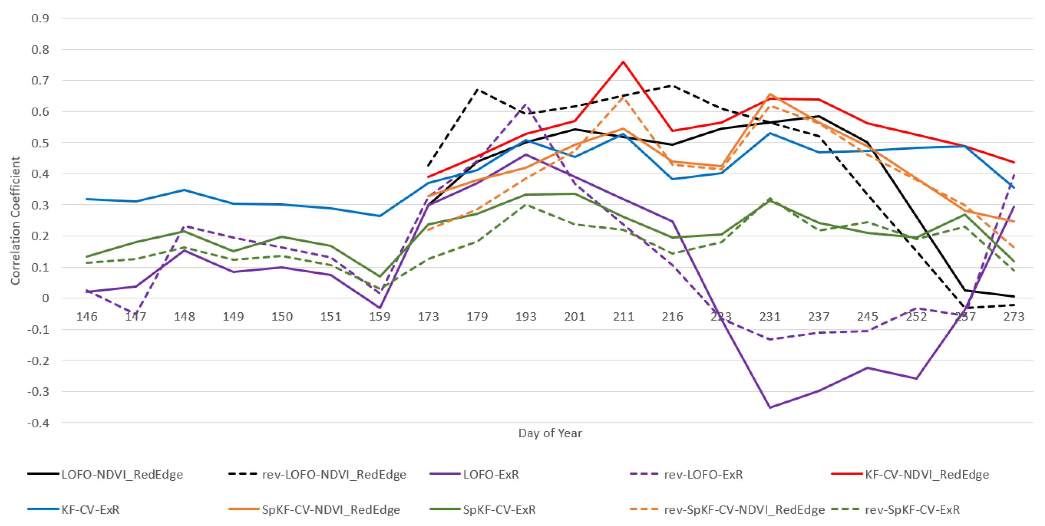
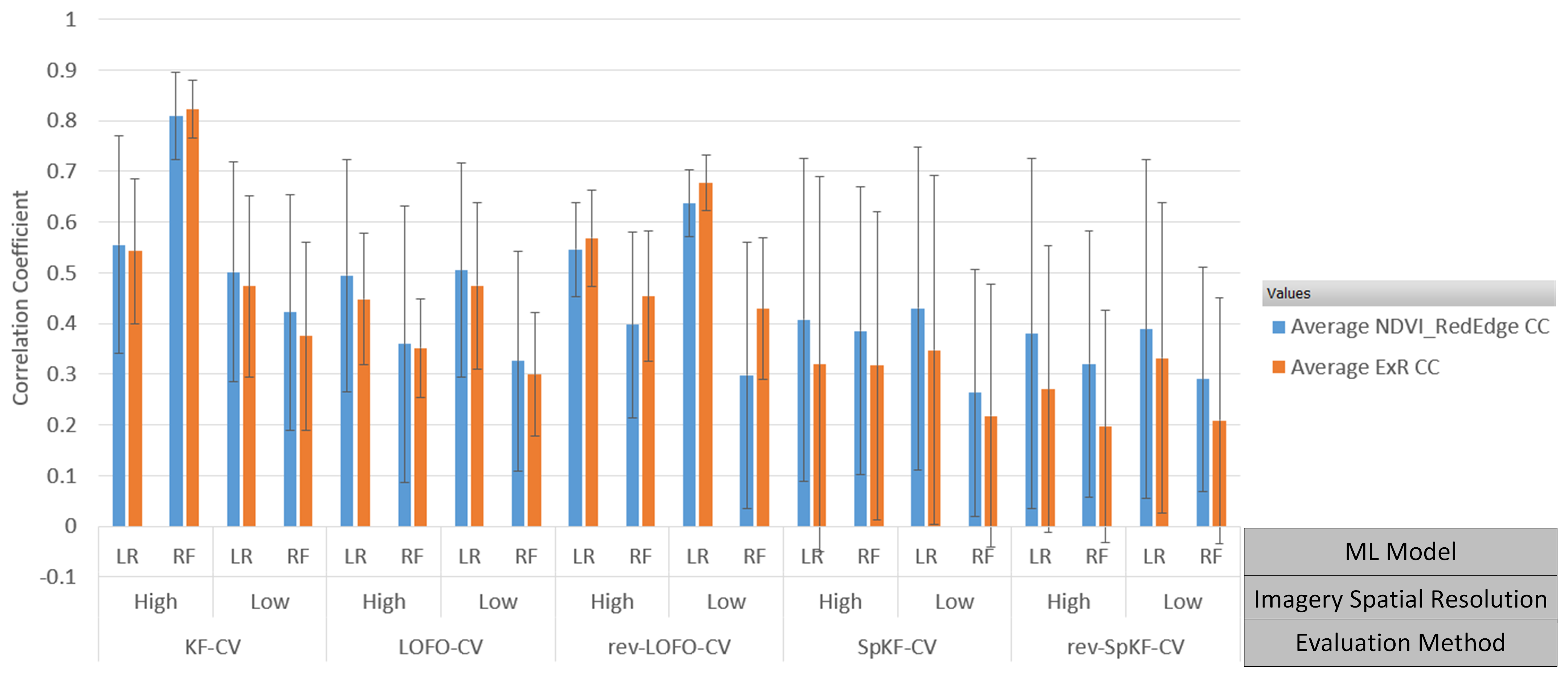

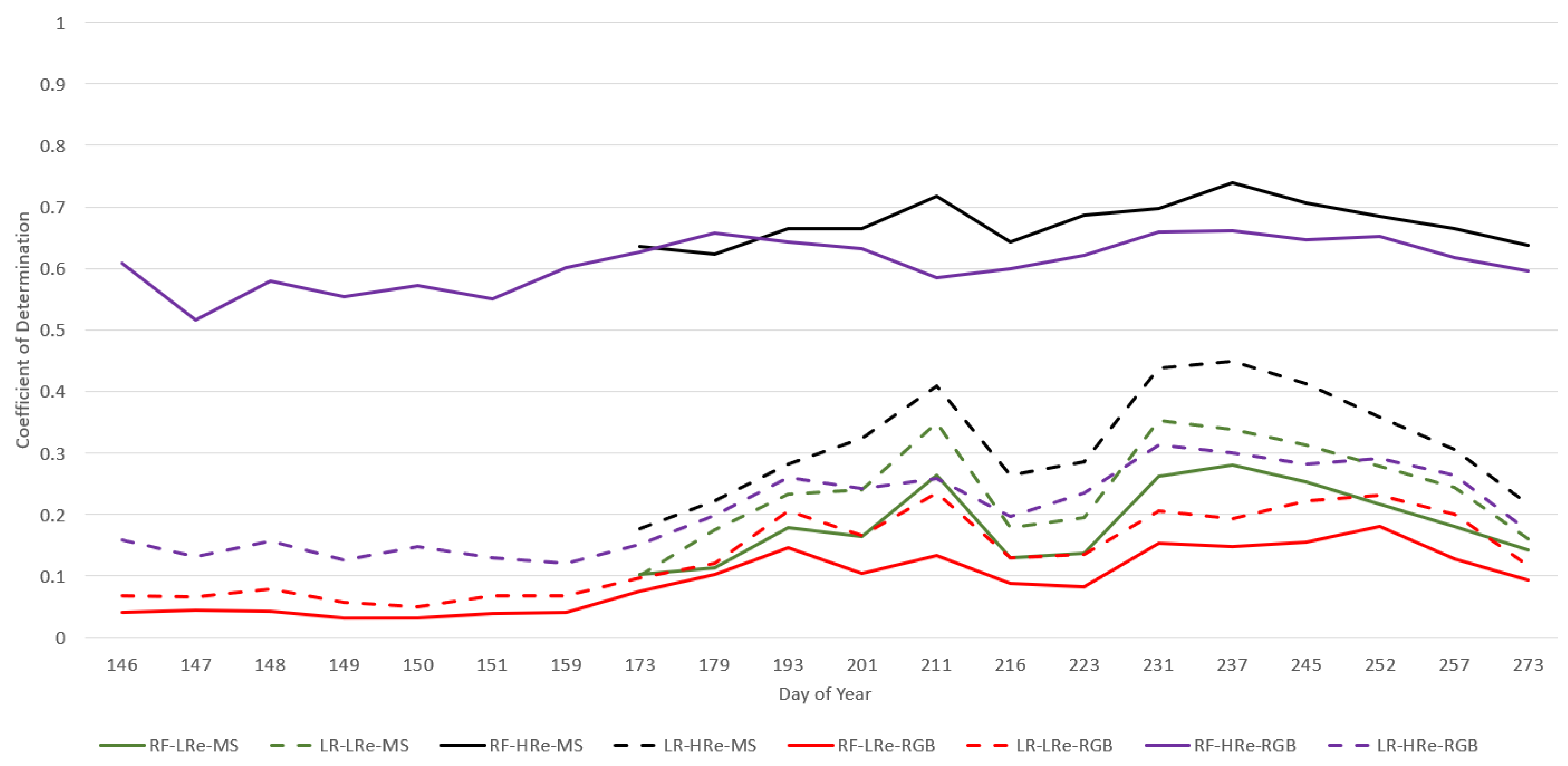
Disclaimer/Publisher’s Note: The statements, opinions and data contained in all publications are solely those of the individual author(s) and contributor(s) and not of MDPI and/or the editor(s). MDPI and/or the editor(s) disclaim responsibility for any injury to people or property resulting from any ideas, methods, instructions or products referred to in the content. |
© 2024 by the authors. Licensee MDPI, Basel, Switzerland. This article is an open access article distributed under the terms and conditions of the Creative Commons Attribution (CC BY) license (https://creativecommons.org/licenses/by/4.0/).