Abstract
Mobile LiDAR technology is a powerful tool that accurately captures spatial information about typical static objects in road scenes. However, the precise extraction and classification of these objects pose persistent technical challenges. In this paper, we employ a deep learning approach to tackle the point cloud classification problem. Despite the popularity of the PointNet++ network for direct point cloud processing, it encounters issues related to insufficient feature learning and low accuracy. To address these limitations, we introduce a novel layer-wise optimization network, LO-Net. Initially, LO-Net utilizes the set abstraction module from PointNet++ to extract initial local features. It further enhances these features through the edge convolution capabilities of GraphConv and optimizes them using the “Unite_module” for semantic enhancement. Finally, it employs a point cloud spatial pyramid joint pooling module, developed by the authors, for the multiscale pooling of final low-level local features. Combining three layers of local features, LO-Net sends them to the fully connected layer for accurate point cloud classification. Considering real-world scenarios, road scene data often consist of incomplete point cloud data due to factors such as occlusion. In contrast, models in public datasets are typically more complete but may not accurately reflect real-world conditions. To bridge this gap, we transformed road point cloud data collected by mobile LiDAR into a dataset suitable for network training. This dataset encompasses nine common road scene features; hence, we named it the Road9 dataset and conducted classification research based on this dataset. The experimental analysis demonstrates that the proposed algorithm model yielded favorable results on the public datasets ModelNet40, ModelNet10, and the Sydney Urban Objects Dataset, achieving accuracies of 91.2%, 94.2%, and 79.5%, respectively. On the custom road scene dataset, Road9, the algorithm model proposed in this paper demonstrated outstanding classification performance, achieving a classification accuracy of 98.5%.
1. Introduction
Streetlights, roadside trees, traffic poles, and other static road elements are fundamental objects for storage and management in the construction of smart cities. Traditional methods of obtaining spatial information on road scenes through manual measurement are inefficient. Currently, with the advantage of capturing detailed 3D point clouds to describe the surrounding environment, the application of mobile LiDAR systems (MLS) in road scene construction is becoming increasingly widespread. Mobile LiDAR systems can rapidly obtain three-dimensional spatial information for static objects in road scenes. They play a crucial role in the spatial analysis of typical features in road scenes, such as traffic sign occlusion [1], the optimization of monitoring areas [2], and streetlight illumination analysis [3], greatly promoting the future development of smart transportation [4] and digital twin [5] construction. The precise classification of static objects in road scenes from vehicle-mounted laser scanning point clouds is the focus of this study.
Currently, deep learning has become a popular research direction in the field of object detection. Initially applied to 2D image data and natural language processing, deep learning gained prominence when the AlexNet model, proposed by Alex et al. [6], reduced the error rate from 25% to 15% in the ImageNet image recognition competition, leading to the popularity of convolutional neural networks. Following this, many researchers extended the use of deep learning to 2D object detection and image segmentation. Representative networks include YOLO, proposed by Joseph et al. [7], and U-Net, proposed by Olaf et al. [8], both showing significant improvements in classification accuracy and efficiency. Thanks to the rapid development of deep learning in the 2D domain, the application of deep learning to 3D point cloud classification has gradually gained popularity. Due to the irregular, unordered, and uneven characteristics of point cloud data, extensive research has been conducted in the field of deep learning for point cloud classification. In recent years, methods of directly processing point clouds have become a research hotspot. The PointNet network proposed by Qi et al. [9] was the first to segment point clouds using raw points but only considered global features. Subsequently, the same team proposed the PointNet++ network [10], which addressed this issue by using hierarchical neural networks. Building upon these two networks, Cheng et al. [11] introduced a novel cascaded non-local module consisting of neighborhood-level, super point-level, and global-level non-local blocks. These blocks collaborate to aggregate local features and enhance the semantic segmentation performance of point clouds. Lu et al. [12] proposed using different aggregation methods for data of the same category and different categories. They introduced a customized module called category-guided aggregation, achieving significant success in point cloud processing.
Due to limitations imposed by the data collection method of mobile radar systems and factors such as occlusion, the point cloud data collected by mobile radar systems are often incomplete, leading to the potential loss of terrain information during the extraction process. Therefore, models for classifying point clouds in road scenes should possess better global feature learning capabilities and robustness. Although the aforementioned methods have achieved good results, most of them have been tested on datasets with complete models publicly available. The accuracy of these methods may be affected when classifying partially occluded point cloud data. Specifically, the popular PointNet++ network employs a hierarchical point set feature learning structure to extract local features, focusing solely on semantic information between points and ignoring basic relationships between layers. Additionally, its feature pooling and integration lack multi-scale features and feature diversity. As a result, it has limitations in learning global features, impacting overall feature learning for the model. Subsequently, many models have been proposed to improve upon this. Lin et al. [13] introduced LGENet, which combines 2D and 3D point convolutions to extract features and learn local features for point cloud segmentation. It ultimately uses a global encoder to leverage contextual information, moderately improving the model’s ability to learn global features. Nie et al. [14] proposed a pyramid architecture that allows information to flow more freely and systematically. While these measures have improved the accuracy of the networks, they overlook the connection between local and global features. They also fail to integrate features at different scales and stages of the network, and the single scale can have an impact on the network’s performance.
To address the aforementioned issues, this paper primarily made improvements in two aspects: firstly, enhancing inter-layer relationships and effectively integrating features between high and low layers. Secondly, adopting a joint pooling method in conjunction with a multi-scale approach to extract features. Additionally, there is a scarcity of publicly available datasets for road scenes on the internet, and synthetic point cloud datasets cannot accurately reflect the features of road scenes. To address this, the paper introduces its own road scene dataset, utilized to validate the effectiveness and generalization capability of the model improvements. The main contributions of this paper can be summarized in two aspects:
- This paper proposes a high-accuracy classification network (LO-Net) for static object point cloud classification in road scenes. The network is mainly composed of three modules: the GraphConv module, the joint module, and the joint point cloud spatial pyramid pooling (J-PSPP) module. The first two modules achieve local feature aggregation and feature learning across multiple layers. Inspired by the spatial pyramid concept in 2D images, the third module introduces the point cloud joint spatial pyramid pooling. It enhances the model’s robustness and improves its classification performance by processing features through multi-scale joint pooling.
- The paper introduces the Road9 road scene dataset based on the Mobile LiDAR system. Unlike public datasets, Road9 contains a certain level of noise compared to synthetic complete datasets, and its point cloud model is more realistic. Additionally, various experiments have been conducted to demonstrate the effectiveness, robustness, and generalization capability of the model.
The remaining sections of this paper are organized as follows. Section 2 provides an overview of the related work in this field. Section 3 presents a detailed explanation of the model’s workflow and the underlying algorithmic principles. Section 4 describes the dataset and provides a comprehensive analysis of the experiments conducted. In Section 5, the experimental results are discussed. Finally, Section 6 provides a summary and conclusion of this paper.
2. Related Work
In this section, the latest methods for point cloud classification based on deep learning are reviewed. Currently, deep learning-based point cloud classification methods can be categorized into four types based on their network structures: multi-view methods, voxelization-based methods, graph convolution-based methods, and point-based methods.
2.1. Methods Based on Multiple Views
The point cloud classification algorithm based on multiple views benefits from the maturity of two-dimensional image classification techniques. Such algorithms simulate human observation of objects from different perspectives by obtaining a series of projected images containing side information from different directions around the three-dimensional point cloud model. Subsequently, two-dimensional image processing techniques are applied to classify these projected images containing point cloud information. Finally, the labels obtained from the segmentation in the two-dimensional views are back-projected onto the three-dimensional point cloud, achieving semantic classification of the point cloud. Classic models such as the Multi-View Convolutional Neural Network (MVCNN) proposed by Su et al. [15] in 2015 generate different 2D views around the point cloud from various “virtual camera” positions. These 2D images are then processed using 2D CNN, and a view-pooling layer is used to fuse features from multiple perspectives to obtain a three-dimensional shape feature representation for classification. Building upon the MVCNN, Feng et al. [16] proposed the GVCNN algorithm, which introduces a global–local view attention mechanism. This mechanism allows the model to focus on more critical global and local information, enhancing the handling of global structure and local details in three-dimensional shapes and improving sensitivity to key features. Different from the approach of projecting from multiple views to obtain two-dimensional projections, Shi et al. [17] first project the three-dimensional shape onto the outer surface of a corresponding cylinder. They then unfold the lateral surface of the cylinder to obtain a single two-dimensional panoramic view. To eliminate the impact of projection rotation, the authors propose a row-wise max pooling layer (RWMP) to obtain rotation-invariant feature representations of the panoramic view. However, this method requires specifying the principal axis for cylindrical projection and is sensitive to the poses of non-normalized objects. For better rotational invariance, Sfikas et al. [18] use the SYMPAN algorithm, which has reflective symmetry, to normalize the pose of three-dimensional models. The models are then projected in both spatial and directional domains, achieving improved performance in three-dimensional object recognition. In summary, these algorithms [19] are relatively efficient. However, due to the involvement of 3D to 2D transformations, the geometric information of point clouds inevitably experiences some loss. Additionally, constrained by the viewpoint, capturing comprehensive features poses challenges, making these algorithms sensitive to occlusion and less suitable for the classification needs of large-scale and complex environmental objects.
2.2. Methods Based on Voxelization
Inspired by convolutional neural networks, algorithms in this category convert point clouds into a spatially uniform voxel grid. Subsequently, they use three-dimensional convolutional neural networks (3DCNN) and similar feature-learning techniques to accomplish classification tasks. Within this category, VoxNet, proposed by Maturana et al. [20], has been a prominent approach capable of directly processing three-dimensional data. However, it is sensitive to the input dimensions. Many researchers have subsequently improved traditional dense voxel methods. For example, Wu et al. [21] proposed the 3D ShapeNets network based on VoxNet, employing a hierarchical structure for multi-level convolution and pooling on three-dimensional data. This gradually extracts higher-level features, enhancing the network’s global feature learning capability. The VoxResNet network introduced by Hao et al. [22] incorporates residual connections to aid the network in better learning deep features. Traditional voxel methods face significant limitations in terms of computer memory when dealing with large amounts of point cloud data. Subsequent research has focused on addressing time and computational cost constraints. Riegler et al. [23] proposed an octree point cloud data structure, where areas with higher point density have finer divisions in the octree representation. This reduces computational costs, improving the network’s adaptability to large-scale three-dimensional data. In addition to improving voxel structures, some studies [24,25] aim to reduce the computational requirements for dense volumetric data after voxelization using sparse convolutions, thereby enhancing computational efficiency. Existing voxelization-based methods effectively address the challenges posed by the unordered and non-structural nature of point clouds. However, determining voxel size poses a significant challenge. Traditional dense voxel representations may quickly exceed computer memory limits, while sparse voxels may result in the loss of valuable information. These factors present challenges to the development of voxel-based methods.
2.3. Methods Based on Graph Convolution
This method combines convolution operations with a graph structure representation, enabling convolutional neural networks to operate on graph structures, capturing dependencies for a more comprehensive understanding of underlying relationships. Kipf et al. [26] proposed Graph Convolutional Networks (GCNs) for feature extraction from graph nodes. With the development of graph convolution, some researchers have applied it to point cloud segmentation tasks. Te et al. [27] introduced the Relation Graph Convolutional Network (RGCNN) for point cloud segmentation, treating point cloud features as graph signals and processing graph-structured data using the point cloud feature matrix and adjacency matrix as inputs. Since earlier algorithms only considered discrete point clouds, neglecting the topological relationships between point clouds, Wang et al. [28] proposed the Dynamic Convolutional Network. This method enhances model performance and robustness through edge convolution networks and dynamically updating the graph structure. Zhang et al. [29] removed the transformation network from the DGCNN to reduce model complexity and proposed a Linked Dynamic Graph for direct segmentation and computation on point clouds. Additionally, many researchers have conducted research in this direction [30,31,32,33]. These algorithms effectively capture the geometric structure of point clouds. However, when facing sparse graphs, the relationships between the model and nodes are susceptible to influences, leading to overfitting. Additionally, these methods primarily focus on nodes in local regions, and improving the learning and understanding of global structures poses a significant challenge.
2.4. Methods Based on Point
Due to spatial information loss in multi-view methods, high computational hardware requirements in voxel-based methods, and difficulties in global feature learning in graph convolution-based methods, point cloud processing methods directly take point clouds as input. They utilize point cloud networks to extract features, preserving the geometric information of input data without demanding high hardware requirements. The pioneering methods in this category are PointNet and PointNet++, proposed by the Qi team. PointNet uses farthest point sampling and constructs a spherical search region to obtain pairs of points in subregions, achieving local feature extraction. However, there is still significant room for improvement in terms of local information and pooling methods. Cortinhal et al. [34] introduced a new module that adds a residual dilated convolution module to the front end of the encoder. This method effectively integrates receptive fields of multiple scales to capture more comprehensive features. Some studies [35,36,37] have also made improvements to it. Recently, attention mechanisms have been widely adopted in deep learning tasks. The fundamental idea is to make neural networks ignore irrelevant information and focus on fine-grained and key features of point clouds, thereby improving the segmentation accuracy and efficiency of the model. Xue et al. [38] proposed the S3Net network, which is based on the Transformer encoder-decoder structure. It uses a sparse residual tower to handle detailed information and extract global features for point cloud segmentation. However, attention mechanisms are susceptible to noise, and improving the robustness of attention mechanisms is one of the challenges in future research.
3. Methodology
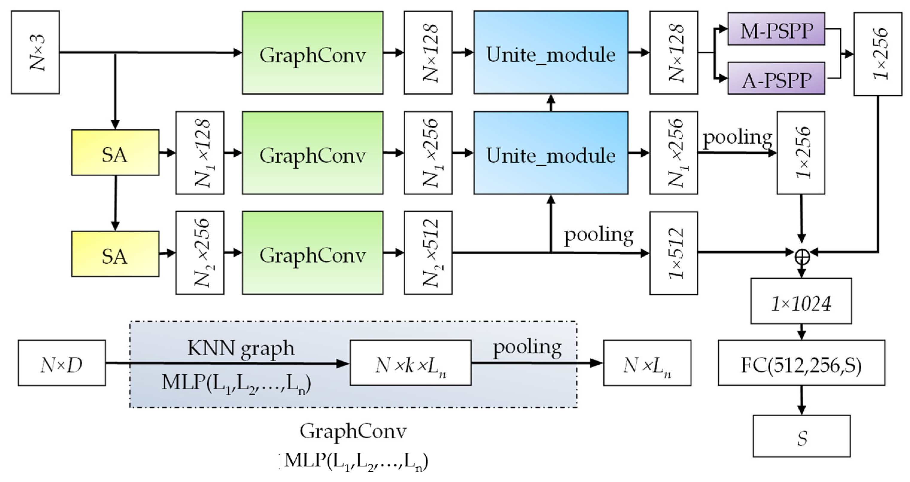
To improve the precision of deep learning in the classification of typical features, this paper introduces the LO-Net network. The network is initially based on a set abstraction (SA) module of PointNet++, which sequentially performs sampling, grouping, and feature extraction to obtain local features of the point cloud. In the network design of this paper, the local features obtained at this stage are considered as the initial features. Since graph convolution can construct local neighborhood graphs within the point set and perform convolution operations on the edges between points to obtain local geometric features, graph convolution is employed for deep information mining and generates intermediate-level features. Subsequently, an upsampling-optimized Unite_module is designed to fuse semantic information with the obtained three layers of local features, enhancing the feature learning capabilities of each layer. Considering that PointNet++ employs single-window feature aggregation through max pooling after feature extraction, with a singular pooling approach, this paper’s LO-Net network constructs a point cloud spatial pyramid joint pooling structure with multiple windows and specific strides. This structure delivers the optimized low-level features to both point cloud spatial pyramid maximum pooling (M-PSPP) and point cloud spatial pyramid average pooling (A-PSPP), combining the features to provide diverse information with both global and local characteristics. Finally, the optimized local features from the three layers are concatenated together to achieve precise point cloud classification.
3.1. Set Abstraction Module
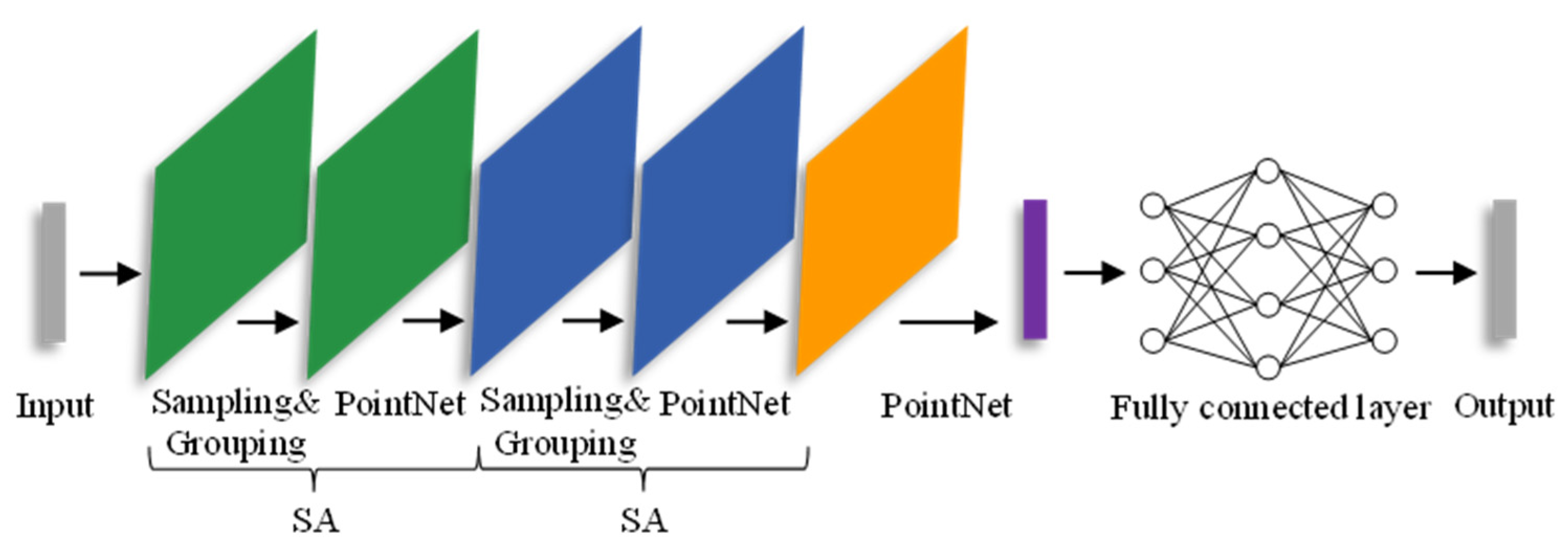
The PointNet++ deep learning network model is developed based on the PointNet network. PointNet utilizes a multi-layer perceptron to extract feature information from point clouds and uses a max pooling layer to extract global features for classification. Although the PointNet network pioneered point cloud processing, it cannot capture the local features of points, and it lacks the ability to analyze point clouds at a finer granularity and generalize well with complex sample data. To address these limitations, the Qi team introduced a hierarchical point set feature learning structure, employing farthest point sampling (FPS) [39] for sampling and designing two “adaptive” solutions for dense and sparse point clouds. This ensures that the sampled points cover the entire sampling space, resolving the issue of uneven point cloud density and achieving end-to-end automated point cloud classification. The structure of the PointNet++ classification network is illustrated in Figure 1.
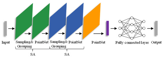
Figure 1.
PointNet++ classification network. The core is the SA module with sampling, grouping, and feature extraction (PointNet) operations. The green, blue, and orange colors represent different stages of feature extraction in the figure, while the purple part represents the fusion of features.
The PointNet++ classification network processes input point cloud data through two SA (set abstraction) modules sequentially and then aggregates features using PointNet, finally calculating the classification scores using fully connected layers. The SA module is the core of the PointNet++ classification network, consisting of three parts: sampling, grouping, and feature extraction. First, it utilizes FPS to downsample the initial point count to . Then, for each sampled point, it clusters the nearest k points within a specified radius using Ball Query, aggregating the input matrix into an matrix. Finally, it employs PointNet for feature aggregation pooling within the sampling region, resulting in local features (where and represent different feature dimensions). The result of the first SA module is input to the next SA module, repeating this process. While the number of central points decreases, the receptive field increases and it captures more feature information, thus obtaining local features of the points.
3.2. GraphConv Module
After processing through two layers of SA modules, the sub-high-level features of the point cloud are obtained. The sub-high-level features contain fewer points, but they possess richer semantic information. In contrast, the low-level features in the input layer contain more points that are closer to the original point cloud, but they have relatively less semantic information. To enable the model to capture both global semantic information and retain local detailed information, it is necessary to fuse high- and low-level features. The fusion process enhances the model’s understanding of objects and scenes. This paper proposes a layered processing approach, leveraging the GraphConv module to obtain enhanced intermediate-level features. This facilitates the subsequent Unite_module module to effectively combine low, intermediate, and high-level features. The basic procedure is as follows: Before the original data enter the first SA module, they undergo GraphConv processing to obtain low-level features. Similarly, the output of the first SA is processed through GraphConv to obtain mid-level features, and the output of the second SA is processed through GraphConv to obtain high-level features. In the subsequent steps, this paper sequentially combines the high-level, mid-level, and low-level features using the Unite_module module to enrich the semantic information.
The GraphConv module aggregates its features through graph convolution, combining the feature vectors of each node and its neighboring nodes in a nonlinear way. This non-linear combination enhances the comprehensive local neighborhood information, strengthening the feature-capturing capabilities. The specific approach involves constructing a directed graph using the K-nearest neighbors (KNN) [40] algorithm, where represents vertices, , is the number of point clouds, and E represents edges formed by KNN. Taking k = 5 as an example, Figure 2 illustrates the feature extraction process of graph convolution. For a selected node , the KNN algorithm selects the five nearest neighboring points {, , , , }. The distances between node and its neighboring points form the edges of the graph, represented by the yellow directional lines in Figure 2, and represents the edge features between node and its neighboring points. Its feature aggregation can be formally represented as Equations (1) and (2).

Figure 2.
Diagram of GraphConv feature extraction when k is set to 5, the white circles represent neighboring points.
Here, represents the adjacent point. represents the target point. denotes a collection of nonlinear functions parameterized by the learnable parameter set . represents the aggregated features of point . Equation (3) represents the process of changing feature space dimensions, where denotes the feature dimension of the original input feature space. This can be achieved by fusing the original feature space to generate a new feature space dimension , achieving the goal of feature learning.
3.3. Unite_Module
The purpose of the Unite_module is to take the features from the upper layer, which contains fewer points but richer semantic information, and attach them to the features of the current layer through a feature upsampling process. This enriches the semantic information of the current layer. The upsampling network architecture can be divided into four categories: pre-upsampling, post-upsampling, stepwise upsampling, and iterative upsampling. In this paper, the pre-upsampling method is employed, which can use interpolation of any size and scale factor compared to other methods, and its learning difficulty is also lower. Figure 3 illustrates the structure of the Unite_module. From Figure 3, it can be observed that the features from the upper layer first undergo an upsampling transformation and are then concatenated with the features of the current layer. Finally, the fused features pass through a multi-layer perceptron (MLP) to produce the output. The new features have two paths: one directly enters the final step, and the other serves as the input for the next Unite_module in the next layer.

Figure 3.
The Unite_module structure shows how features can be semantically optimized.
By using upsampling, the lower-level features are transferred to the upper layer, allowing the lower-level features to receive richer semantic information through this combination of high- and low-level features. In this module, the upsampling is achieved through a reverse interpolation method. A Euclidean distance matrix and weighting coefficients are computed based on the points between adjacent layers. For each point to be interpolated, three of the nearest neighboring points are selected, and the weighted average of their features is calculated as the feature of the interpolated point. These interpolated features are stacked with the features from the previous layer using skip connections to perform feature upsampling. The weighting coefficients are determined by taking the reciprocal of the distances of each point and dividing it by the sum of the reciprocals of the distances of the three nearest neighboring points. Through interpolation, the point count in the lower-level features is restored to match the point count in the upper-level features. This combines the features into fused features, and the mathematical formulas for the process of inverse interpolation are shown in Equations (4) and (5).
In the equation, represents the feature interpolation of the point to be interpolated, where is a known point, is an unknown point, and represents the feature value of the known point. M represents the number of known points. represents the weight value, which is the reciprocal of the Euclidean distance between the unknown point and the known point. denotes the set of known point cloud regions.
3.4. J-PSPP Module
In deep learning networks, pooling functions are commonly used to process features, resulting in features with dimensions of . For example, in the PointNet network, after multiple layers of convolution operations, point cloud features are dimensionally elevated to N × 1024. Following this, max pooling is employed to obtain global features of size 1 × 1024, which are then replicated for N points. Finally, these features go through fully connected layers to yield classification scores. However, max pooling utilizes a fixed pooling window size N, and can only integrate global features, lacking detailed descriptions of local point cloud features. Inspired by the spatial pyramid pooling (SPP) [41] used in the pixel domain of 2D images, this paper introduces a point cloud spatial pyramid joint pooling module (J-PSPP) to enhance the network. For the conventional point cloud spatial pyramid pooling, a multi-window pyramid pooling approach can be adopted, allowing the final features to include both global and fine-grained local information, as shown in Formula (6).
In the equation, represents different pooling window sizes. represents the feature information learned by the network. represents the pooling method employed by the network. represents the feature concatenation operation, which combines and integrates the features obtained from different pooling windows.
As observed in Figure 4, cones of varying sizes and colors represent pyramid pooling windows with sizes . The PSPP (point cloud spatial pyramid pooling) structure enables the pooling and integration of features under multiple window sizes, ultimately resulting in features of dimensions . PSPP achieves the aggregation of local information with different characteristics by concatenating network features obtained from various scale neighborhoods. Compared to conventional pooling operations, PSPP offers the advantage of being non-parametric, effectively enhancing the network’s ability to learn point cloud features.
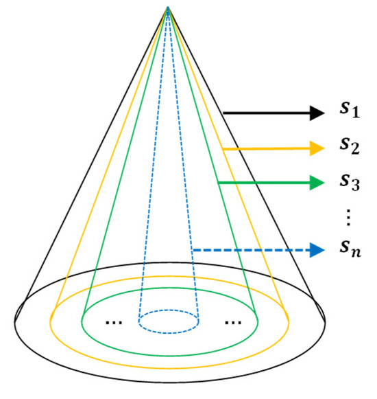
Figure 4.
Structure of point cloud space pyramid pooling.
This paper simultaneously applies PSPP to both max pooling and average pooling, achieving the joint complementary utilization of the two pooling methods. This compensates for the limitations of a single pooling method, resulting in the J-PSPP module. The formal expressions of M-PSPP and A-PSPP are represented in Equations (7) and (8), where represents the max pooling operation, represents the features after M-PSPP pooling, represents the average pooling operation, and represents the features after A-PSPP pooling.
Point cloud spatial pyramid joint pooling is represented as shown in Equation (9), which represents the result of joint pooling. The J-PSPP module aggregates features of point cloud data through different windows and pooling methods, ultimately obtaining more fine-grained feature information.
3.5. LO-Net Overall Network Architecture
The overall structure of the LO-Net classification network is illustrated in Figure 5. In the figure, represents the number of point clouds, and is the feature dimension. The raw point cloud data, , has two pathways as input to the network. The first pathway is directly fed into the GraphConv module, which extracts dimensional feature information, representing the low-level features. Since the input data include all the point clouds, they capture both global and local information. The blue dashed box in the lower-left corner of Figure 5 depicts the GraphConv structure. It involves a KNN graph, representing a k-nearest neighbor point search for all points in the set, constructing the neighborhood region. Subsequently, edge information is extracted through MLP () with shared weight attributes, where () represents the number of neurons in each layer. Finally, the pooled operation aggregates the dimensional feature results. The second pathway of data is sent to the SA (set abstraction) module for local point feature extraction. The result of the first SA module is dimensional information (N1 represents the downsampled point count, ). It then undergoes GraphConv to extract local geometric information, resulting in , representing the mid-level features. The result of the second SA module undergoes GraphConv and yields local features ( represents the point count after downsampling , ), representing the high-level features. The high-level features and mid-level features are processed by the Unite_module to perform upsampling, obtaining mid-level features strengthened by semantic information. Similarly, the Unite_module processes the low-level and mid-level features, acquiring enhanced low-level features. Currently, is sent to M-PSPP and A-PSPP for multi-scale pooling, and their pooled results are concatenated, yielding dimensional information that encompasses both multi-scale local features and global features. Finally, this feature, the mid-level feature () after pooling, and the high-level feature () after pooling are concatenated to obtain information with the ability to harness multiple features. After processing through the fully connected layer, the network produces classification results for categories.

Figure 5.
LO-Net classification network (key modules are shown in different colors except for the lower left corner).
4. Experiment
4.1. Preparation for Experiment
The experimental hardware environment consists of an Intel Core i7-9700F processor, an RTX 2060 graphics card with 6 GB of RAM, and 16 GB of system memory (RAM). The software environment includes Ubuntu 16.04 (64-bit), Windows 10 (64-bit), CUDA 10.1, cuDNN 7.5, TensorFlow 1.13, and Python 3.7.
4.2. Network Parameter Settings
Based on the experimental environment in this paper, the network configuration is set according to the parameters provided by the PointNet++ network. In this paper, the improved network employs the ReLU activation function; the loss function is chosen to be cross-entropy; the optimization algorithm is the Adam optimizer with the number of optimization iterations (Epoch) set to 250; training is conducted using the momentum gradient descent method, with the momentum parameter set to 0.9; and to expedite network training, alleviate overfitting, and enhance the generalization ability of the neural network, a dropout rate of 0.5 is introduced between each fully connected layer. The learning rate, which determines the magnitude of parameter updates during network learning, is set to 0.001, and the decay rate is set to 0.7. To ensure the network converges as quickly as possible within the available memory, the batch size is set to 8. The number of sample points for network learning is set to 2048, with the same sampling and neighborhood point numbers as in the PointNet++ network to ensure there are enough points for feature learning.
4.3. Experimental Dataset
Considering that most studies have focused on public datasets, we transformed the point cloud data collected by mobile LiDAR into a dataset suitable for network training and conducted classification research based on public datasets and this dataset.
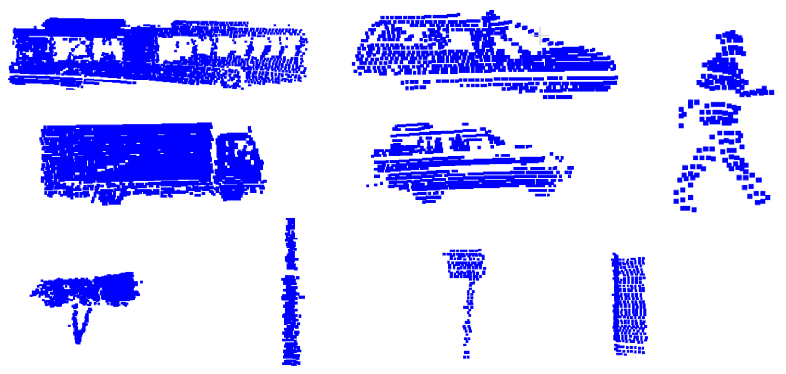
- Public datasets: To explore the feasibility and robustness of the improved deep learning network model in classifying typical features in road scenes, this paper decided to conduct experiments using internationally recognized standard datasets, namely ModelNet Dataset [10] and the Sydney Urban Objects Dataset [42]. ModelNet Dataset includes ModelNet10 and ModelNet40. The ModelNet40 public dataset comprises 9843 training models and 2468 test models, totaling 12,311 rigid 3D models. The choice of this dataset is due to its noise-free nature, allowing for an accurate reflection of the feasibility of model improvements. Visualizations of the ModelNet dataset samples are presented in Figure 6. The Sydney Urban Objects Dataset (Suo Dataset) was collected using Velodyne HDL-64E LiDAR scans of various common urban road objects in the Central Business District (CBD) of Sydney, Australia. The dataset includes 631 scans of different object categories, covering vehicles, pedestrians, signs, and trees. This dataset represents a sparse point cloud model with a significant degree of point density unevenness. The selection of this dataset allows for testing the robustness and generalization ability of model improvements. Visualizations of the Sydney Urban Objects Dataset samples are presented in Figure 7.
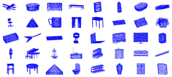
Figure 6.
Forty different categories of 3D point cloud models in the ModelNet dataset.
Figure 6.
Forty different categories of 3D point cloud models in the ModelNet dataset.


Figure 7.
Partial visualization of the Sydney Urban Objects Dataset.
Figure 7.
Partial visualization of the Sydney Urban Objects Dataset.
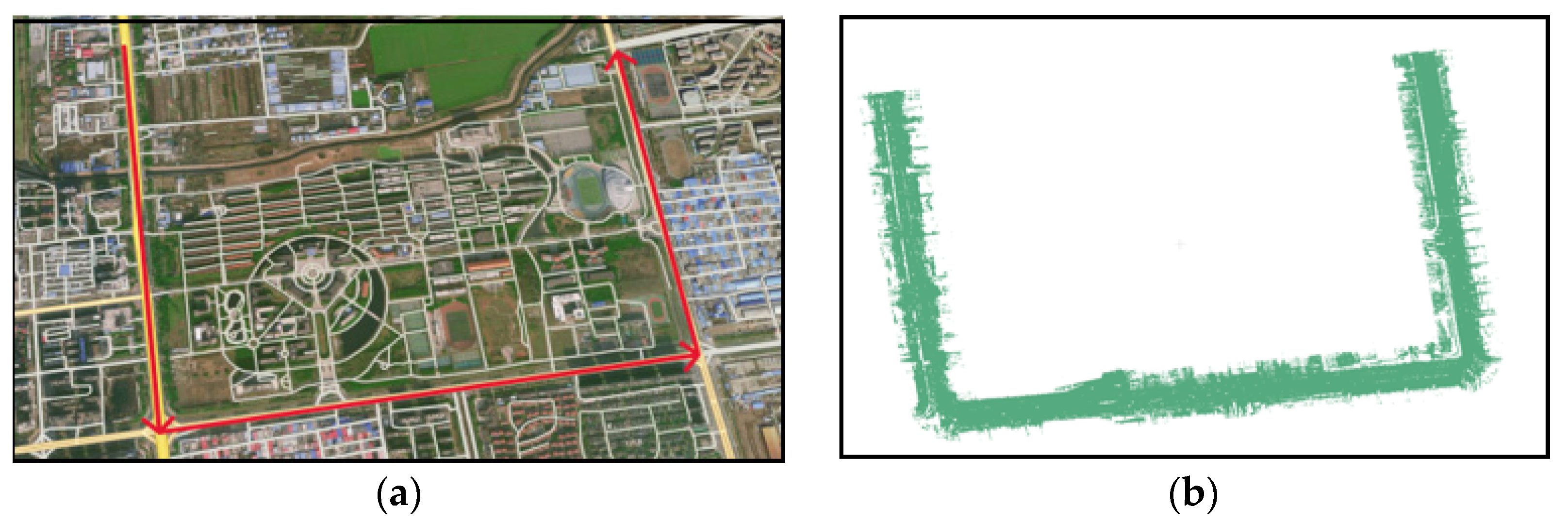
- Road9 dataset: The Road9 dataset was created by collecting point cloud data from a circular road in Shanyang District, Jiaozuo City, Henan Province, using the SSW-3 mobile LiDAR system. As shown in Figure 8, it is the overall visualization of the study area’s remote sensing image Figure 8a and the original point cloud Figure 8b. In Figure 8a, the highlighted red section represents the main research segment, depicting a complex road scene.
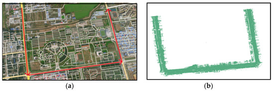
Figure 8.
Road9 dataset research overview: (a) remote sensing image of the study area, the red arrows indicate the data acquisition route. (b) visualization display of the partial original mobile LiDAR point cloud data.
Figure 8.
Road9 dataset research overview: (a) remote sensing image of the study area, the red arrows indicate the data acquisition route. (b) visualization display of the partial original mobile LiDAR point cloud data.
The process of converting LiDAR data into training data for the network is mainly divided into two major parts. The first part is raw data preprocessing, which is further divided into four steps: data clipping (Figure 9a), data denoising (Figure 9b), data segmentation, and ground point removal (Figure 9c). A partial workflow is illustrated in Figure 9. Data clipping focuses on obtaining road scene data within buildings. Subsequently, noise reduction is achieved through the Statistical Outlier Removal (SOR) filter. To alleviate computational pressure in subsequent data processing, Terra Solid v8 software is used to segment the data, with overlapping sections to ensure that extracted features are not disrupted or split. Finally, a cloth simulation filtering algorithm (CSF) [43] is employed to separate ground points, completing the data preprocessing. The second part involves applying a multi-stage clustering segmentation algorithm [44] to extract objects from the non-ground point cloud. Subsequently, the dataset format is modified to control the number of points to 2048 and labeled. Finally, the data are written to an.h5 file in a 7:3 ratio, creating the Road9 dataset. The Road9 dataset comprises 2670 object models belonging to nine different categories, with 1866 training models and 804 test models. The dataset includes nine categories of objects: 707 streetlights, 205 traffic signals, 970 roadside trees, 170 poles, 241 traffic signs, 52 garbage cans, 57 bus waiting shelters, 47 guardrails, and 221 motor vehicles. In real road scenes, point cloud data are often incomplete due to occlusion. The visualization of the dataset attempts to select complete 2D representations for display, Partial data are often represented as data from only one side, as shown in Figure 10. The visualization of the Road9 dataset and a partial comparison with the Sydney Urban Objects Dataset (SUO Dataset) are presented in Table 1.

Table 1.
Visualization of the Road9 dataset and a partial comparison with the SUO Dataset.

Figure 9.
Data preprocessing schematic diagram. (a) Schematic diagram of road scene data clipping, with red lines indicating segmentation; (b) effect diagram of road scene data denoising; (c) effect diagram of ground filtering processing, the ground is represented in blue.
Figure 9.
Data preprocessing schematic diagram. (a) Schematic diagram of road scene data clipping, with red lines indicating segmentation; (b) effect diagram of road scene data denoising; (c) effect diagram of ground filtering processing, the ground is represented in blue.
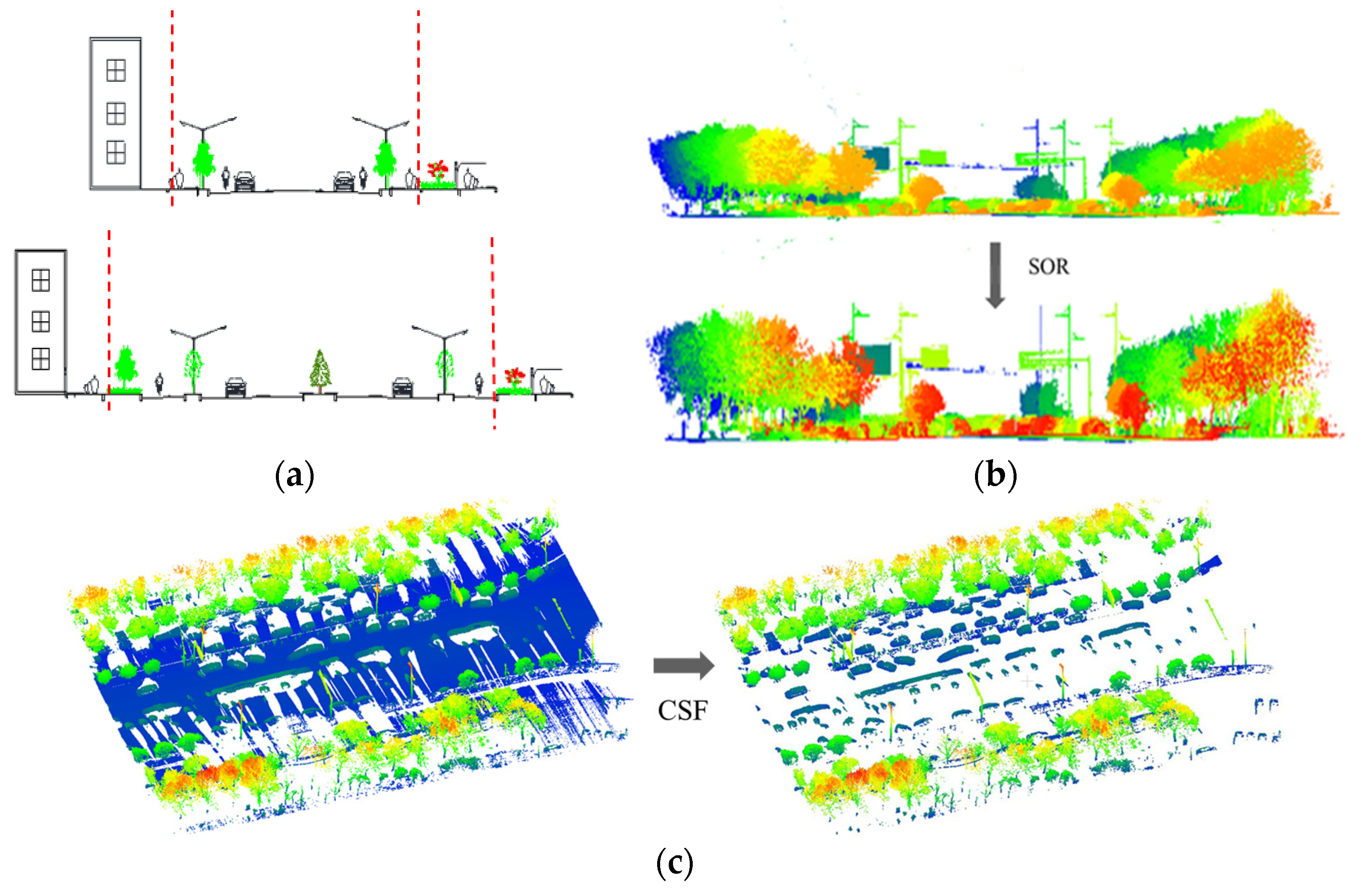

Figure 10.
Incomplete model lateral views of road scenes, (a) overhead view of a sample traffic signal, (b) rear view of a sample car.
Figure 10.
Incomplete model lateral views of road scenes, (a) overhead view of a sample traffic signal, (b) rear view of a sample car.

4.4. Evaluation Index
The classification results for the same dataset may vary between different models. Therefore, this paper uses overall accuracy (OA), mean accuracy (MA), F1-score, and the Kappa coefficient as evaluation metrics for comparative analysis of the classification performance of multiple models.
- Overall accuracy: This refers to the ratio of the number of correctly classified samples to the total number of samples. A higher score indicates better classification performance of the network. The formula is as follows (Equation (10)).In the equation, represents the number of target categories; represents the number of samples correctly classified in class i; and represents the number of samples of class i predicted as class j.
- Mean accuracy: The average of the independent classification accuracies for each category, divided by the number of target categories. A higher score indicates better classification results for each category. The formula is as follows (Equation (11)).
- F1-score: A weighted harmonic mean that takes both recall and precision into account, used for a comprehensive evaluation of network performance. The formula is as follows (Equation (12)).precision refers to the proportion of correct classification numbers in the sample results. The calculation formula is shown in Equation (10). recall is the recall rate, which refers to the proportion of the number of correct classifications in a sample classification result. The calculation formula is shown in Equations (13) and (14).
The meanings of the relevant parameters are shown in Table 2.

Table 2.
Definition of true positive (TP), true negative (TN), false positive (FP), and false negative (FN).
- Kappa coefficient: This refers to the index used to evaluate the overall classification accuracy of the network model. The larger the value, the stronger the classification performance of the network and the better the classification effect. The calculation formula is shown in Equations (15) and (16).
4.5. Experimental Analysis of Public Dataset
4.5.1. Graph Convolution K-Value Selection Analysis
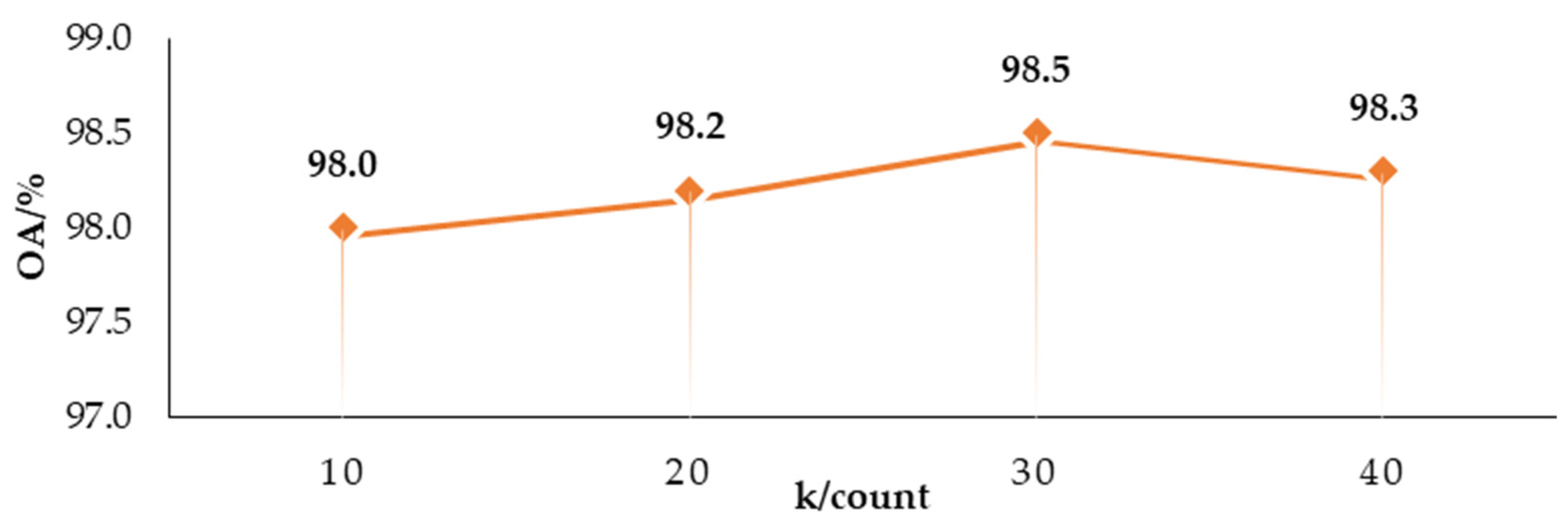
The feature extraction performance of graph convolution depends on the number of k-nearest neighbors. To assess the impact of different k-values on the network’s performance, a comparison of classification accuracy was conducted for various k-values, as shown in Figure 11.
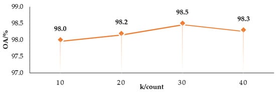
Figure 11.
OA value of LO-Net network affected by different k values of GraphConv.
From Figure 10, it can be observed that the overall accuracy is the lowest when k is set to 10, indicating that having too few neighboring points does not effectively capture local geometric features. With an increase in the value of k, the overall classification performance improves. When k is set to 30, the accuracy reaches a relatively high value. However, when k is set to 40, the network’s classification accuracy decreases, and it also increases the computational load and runtime. In summary, choosing a k value that is either too small or too large can lead to a decrease in the network’s classification performance. Therefore, the choice of the k value is crucial, and in this study, LO-Net selects k = 30.
4.5.2. Analysis of Public Dataset Experiments
This paper first conducts an accuracy analysis on the public dataset ModelNet. From Table 3, it can be observed that the accuracy of the LO-Net network is equal to or greater than that of the Point and PointNet++ networks in 27 categories, indicating that this network has stronger classification capabilities for individual objects.

Table 3.
The classification accuracy of 40 typical objects in the publicly available ModelNet40 dataset evaluated by the PointNet, PointNet++, and LO-Net networks.
To demonstrate the effectiveness and generalization capability of the improved LO-Net classification network, we evaluated it using the publicly available ModelNet40, ModelNet10, and Sydney Urban Objects Dataset. We compared its accuracy against the PointNet and PointNet++ networks. As shown in Table 4, on ModelNet40, LO-Net achieved overall accuracy and mean accuracy of 91.2% and 88.9%, respectively. These values are 2.6% and 2.9% higher than PointNet and 1.4% and 0.9% higher than PointNet++. On ModelNet10, LO-Net attained an overall accuracy of 94.2% and a mean accuracy of 94.1%, surpassing PointNet by 2.6% and 2.9%, and PointNet++ by 1.9% and 1.8%. Moreover, on the Sydney Urban Objects Dataset, LO-Net demonstrated an overall accuracy of 82.4% and a mean accuracy of 79.9%. These values are notably higher compared to PointNet (18.7% and 2.8% higher) and PointNet++ (1.9% and 3.1% higher). LO-Net exhibits stronger classification performance across different datasets. Additionally, we conducted experiments with the point-based method PointGrid on public datasets, achieving 90.1%, 87.4%, 78.3%, and 77.4% accuracy on ModelNet40 and Sydney Urban Objects Dataset, respectively, all of which are lower than LO-Net’s performance. While the overall accuracy of PointGrid differs significantly from LO-Net, its average accuracy is similar to LO-Net. This indicates that the LO-Net network may have lower accuracy in certain specific categories, which is the direction in which we aim to improve. In conclusion, LO-Net exhibits stronger classification performance across different datasets.

Table 4.
Comparison of OA and MA of public datasets in PointNet, PointNet++, PointGrid, and LO-Net.
4.6. Experimental Analysis of Road9 Dataset
Table 5 displays the recall, precision, and F1-score values for nine typical land cover samples in the PointNet, PointNet++, and LO-Net models on the Road9 dataset.

Table 5.
Recall, precision, and F1-score values of 9 typical ground objects in the Road9 dataset in PointNet, PointNet++, and LO-Net networks.
Analyzing the data in the table, it is evident that the LO-Net network achieved better classification results across all three evaluation metrics when compared to the PointNet and PointNet++ networks. The following Table 6 shows the identification results of some typical landmarks.

Table 6.
The recognition results of some typical landmarks on the Road9 dataset. The data type labels refer to Table 1.
Based on the data analysis in Table 5 and Table 6, the overall structure of motor vehicles is completely distinct from other landmarks. Despite the presence of some deficiencies, multiple network models can accurately identify and classify them. However, for street lamp samples with poor completeness, both the PointNet and PointNet++ networks experience classification errors, while the LO-Net network, relying on its strong feature extraction capabilities, can accurately identify them. Traffic lights suffer from issues such as incompleteness and sparse point density. Additionally, in real road scenarios, the contours of traffic lights are similar to those of traffic signs, leading to all three networks being unable to fully learn their features, resulting in misclassification as traffic signs or pole-like objects. For individual long guardrail samples, under the condition of ensuring the same input point number, the PointNet and PointNet++ networks cannot accurately learn unique features, leading to the misclassification results of “3Pole” and “traffic signal lamps”. In contrast, the LO-Net network conducts in-depth exploration at the local feature level, demonstrating a more proficient grasp of the geometric semantic information of landmarks and achieving correct labeling. Bus stop shelters, located at the edge of the main road with close proximity and low occlusion to the onboard LiDAR system, possess unique geometric structures, allowing all network models to achieve 100% classification accuracy.
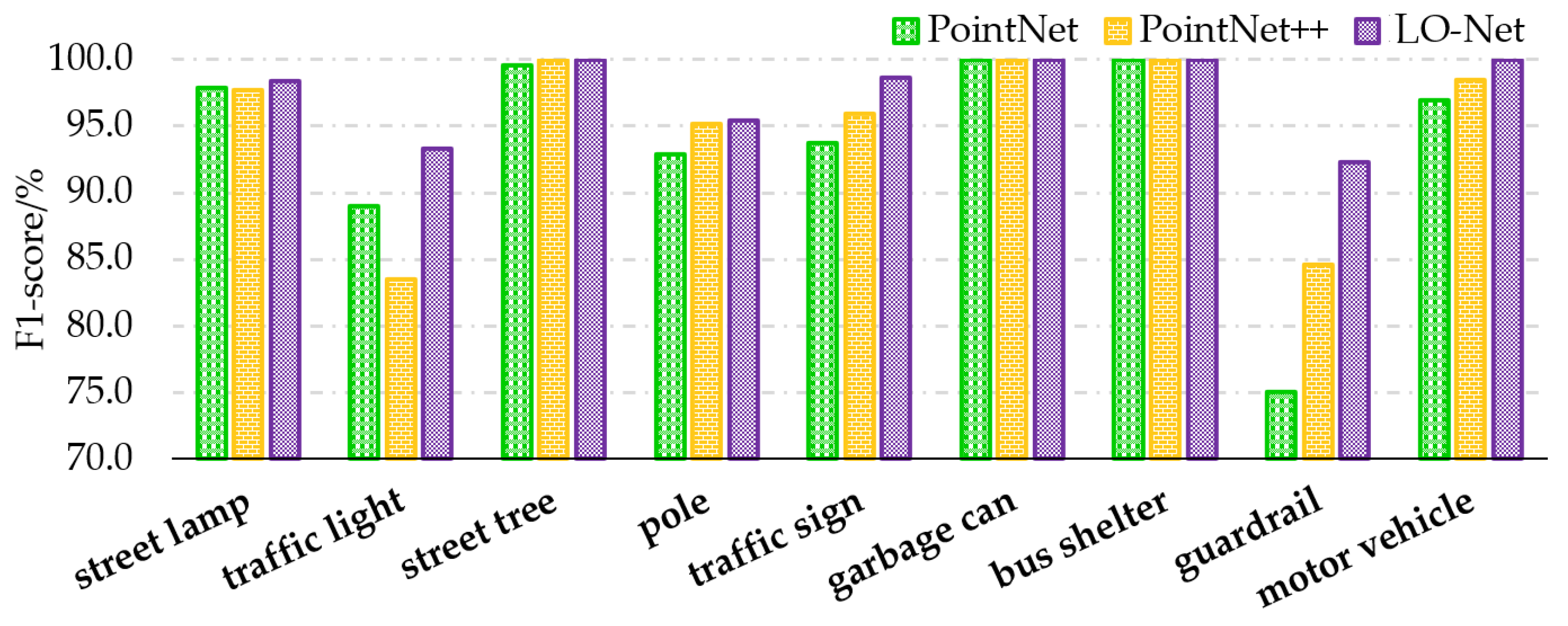
As for the F1 values in Table 5, which offer a more comprehensive reflection of single-sample classification performance, the results for different land cover types are as follows: road lamps achieved an F1 score of 98.4%, traffic signal lamps scored 93.3%, road trees scored 100%, line poles scored 95.4%, traffic signs scored 98.6%, garbage bins scored 100%, bus stops scored 100%, guardrails scored 92.3%, and motor vehicles scored 100%. Compared to the PointNet and PointNet++ networks, all samples showed higher F1 values, indicating improved classification performance for individual samples. Analyzing the characteristics of each land cover sample individually, as can be seen from the bar chart in Figure 12, it becomes clear that road trees, garbage bins, bus stops, and motor vehicles have relatively simple and distinct shapes, resulting in high F1 scores, all achieving 100% classification F1 values in the LO-Net network. Road lamps rely on their arms or single-arm lamp heads to distinguish themselves from other samples, achieving a 98.4% F1 score. Traffic signs come in multiple varieties, but their head components exhibit distinctive cubic features, contributing to a 98.6% result. Line poles can be either long and straight or have protruding features, which sometimes resemble sparse or incomplete pole-like land features, resulting in a 95.4% F1 score. Traffic signal lamps have diverse types, including cameras, pedestrian crossing signal lamps, intersection signal lamps, and central road signal lamps, which exhibit various shapes. Guardrails are long and straight with multiple protruding structures, making them susceptible to misclassification as traffic signal lamps or line poles, and there are fewer instances of this sample compared to others. Consequently, traffic signal lamps and guardrails achieved the lowest F1 scores.
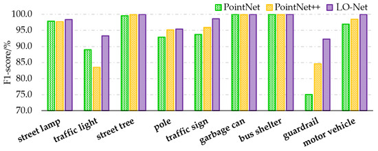
Figure 12.
Classification F1-score comparison of 9 samples in the PointNet, PointNet++, and LO-Net networks.
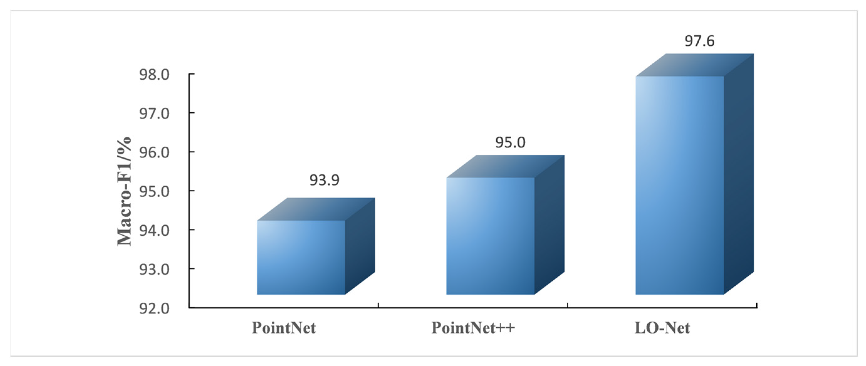
For the classification task on the Road9 dataset, the F1-score describes the performance of individual samples, essentially binary classification. To capture the overall performance of the network for multi-class tasks, this study employs the macro-average Macro-F1 for comparative analysis, as shown in Figure 13. Macro-F1 is the average of the F1-scores for all samples. It is evident from the chart that the LO-Net network achieves a score of 97.6%, consistently higher than the Macro-F1 values of the PointNet and PointNet++ networks.
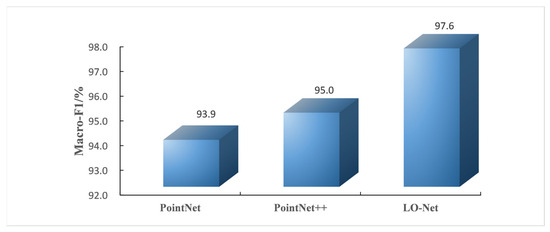
Figure 13.
Comparison of Macro-F1 scores for PointNet, PointNet++, and LO-Net networks.
To provide a more comprehensive analysis of the overall classification performance of the LO-Net network in this study, metrics such as overall accuracy (OA), mean accuracy (MA), and the Kappa coefficient were used for evaluation. As shown in Table 3, the LO-Net network achieves an OA of 98.5% and an MA of 97.0%. Compared to the PointNet network, it exhibits improvements of 2.2% and 4.3%, respectively, while compared to the PointNet++ network, it shows improvements of 1.3% and 3.0%. These results demonstrate a significant enhancement in classification accuracy. Furthermore, the Kappa coefficient of 0.981 indicates that the optimization of the network with GraphConv, Unite_module, and J-PSPP allows for a more detailed extraction of feature information for land objects, resulting in a substantial improvement in classification accuracy.
This confirms the strong classification performance of the LO-Net network on the Road9 dataset, as evident from Table 5 and Table 7, as well as Figure 9 and Figure 10.

Table 7.
Comprehensive comparison of PointNet, PointNet++, and LO-Net networks on OA, MA, and Kappa coefficients.
4.7. Ablation Experiment
To verify the impact of the point cloud spatial pyramid pooling (PSPP) structure on the network’s classification performance, this paper conducted ablation experiments to compare accuracy under various conditions. As shown in Table 8, the overall accuracy obtained with single max pooling is 98.0%, and with single average pooling, it is 97.8%. Although the overall accuracy with PSPP is also 98.0%, the mean accuracy is improved by 0.4% and 0.6% respectively. This demonstrates that adopting the PSPP structure allows for diverse feature information, resulting in higher accuracy compared to single pooling methods.

Table 8.
Comparison of precision of single pooling and combined pooling and comparison of network classification accuracy under different J-PSPP structures.
Analyzing the data in Table 3, it is evident that the window size and quantity of the point cloud spatial pyramid pooling (PSPP) structure also have a certain impact on network accuracy. Specifically, for the N/1, N/2, N/4, N/8, and N/16 window types in the point cloud spatial pyramid max pooling structure, the overall accuracy is 98.3%, and the mean accuracy is 96.6%. Similarly, for the same structures with point cloud spatial pyramid average pooling, the overall accuracy is 98.2%, and the mean accuracy is 95.9%. This indicates that constructing the PSPP structure is more effective than the conventional single-window pooling method. Furthermore, under the N/1, N/2, N/4, N/8, and N/16 window structures of the point cloud spatial pyramid pooling, it is possible to further enhance the network’s accuracy, achieving an overall accuracy of 98.5% and a mean accuracy of 97.0%. While the networks under the N/1, N/2, N/4, N/8, N/16, and N/32 window structures have the same overall accuracy of 98.5%, the mean accuracy decreased by 0.3%. In conclusion, the J-PSPP structure in N/1, N/2, N/4, N/8, and N/16 window structures achieves the best classification performance for the custom-made Road9 dataset.
To investigate the influence of the GraphConv, Unit_module, and J-PSPP modules on the network, various combinations were analyzed through ablation experiments. It should be noted that when Unit_module was not used, GraphConv only processed high-level features, and J-PSPP was placed after the high-level features. As evident from Table 9, combining two modules resulted in a more significant improvement in accuracy compared to using a single module. The combination of all three modules optimized and enhanced the network’s learning capability in the best way, resulting in an overall accuracy and mean accuracy of 98.5% and 97.0%, respectively.

Table 9.
Influence of different module combination modes on network accuracy (note: when Unit_module is not used, GraphConv only processes high-level features and J-PSPP is placed behind the high-level features).
5. Discussion
This paper investigates the classification of improved deep learning networks for typical road scene objects. The experiments in Section 3 demonstrate the effectiveness, robustness, and generalization capability of the LO-Net classification network. Firstly, experiments are conducted on synthetic datasets (ModelNet40 and ModelNET10). As shown in Table 9, in environments where point cloud models are complete and free of noise, LO-Net achieves higher accuracy compared to PointNet, PointNet++, and PointGrid, with improvements of 2.6%, 2.9%, 1.65%, 1.35%, 1.1%, and 1.5%, respectively. This reflects the effectiveness of the improved LO-Net classification network. Secondly, on the Sydney Urban Objects Dataset, due to the limited training samples, models generally achieve lower accuracy. PointNet and PointGrid networks, neglecting relationships between layers, result in the loss of structural data in lower-level features, making them less descriptive and sensitive to noise. In contrast, LO-Net fully utilizes features between layers, expanding the receptive field, and thus, LO-Net demonstrates higher overall accuracy and better robustness compared to other networks. On the Road9 dataset, LO-Net achieves an overall accuracy of 98.5% and a mean accuracy of 97%, outperforming PointNet by 2.2% and 4.3%, and PointNet++ by 1.3% and 3%, highlighting the strong generalization capability of LO-Net. In conclusion, LO-Net exhibits superior classification performance on both public datasets and realistic road scene datasets.
Analyzing the reasons behind this, PointNet is a pioneering network that directly processes point clouds but can only obtain global features of point clouds through multiple convolutions, lacking the description of local features. PointNet++, on the other hand, continuously samples, groups, and extracts features within the point set, resulting in a larger receptive field and more feature information, allowing it to capture local features of point clouds. However, this network focuses solely on semantic information between points and lacks the analysis of “edge” properties between point sets. The LO-Net network proposed in this paper absorbs the advantages of PointNet++’s hierarchical feature learning structure and builds multiple modules for feature optimization and enhancement.
- GraphConv conducts learning between adjacent points in the point set, allowing the aggregation of edge features near the central point, greatly absorbing geometric information in the local domain. This enables the network to learn more point cloud features.
- Unite_module integrated after hierarchical feature learning employs upsampling to gradually restore the low-point count layer features to the previous layer, progressively refining the semantic features of each layer and making the features learned at each level more comprehensive.
- J-PSPP pools the final features obtained, using pyramid pooling to learn features from different spatial regions. This combined with joint pooling allows the network to acquire multi-scale and multi-style features that encompass both local and global characteristics.
The hierarchical optimization involving multiple modules enhances the point cloud learning ability, leading to increasingly robust feature extraction capabilities and ultimately achieving better classification performance.
6. Conclusions
This paper introduced an improved deep learning model called LO-Net, which effectively improved classification accuracy for typical road scene objects. It extracted typical objects from preprocessed point clouds obtained from a mobile LiDAR system, creating the necessary datasets for the study. Based on the SA module of the PointNet++ network, the paper transformed and optimized the network using three modules, GraphConv, Unit_module, and J-PSPP, designed to combine multiple feature learning methods in a layer-wise optimized network for dataset classification. Experimental results demonstrated that the LO-Net network performed well on public datasets, achieving an overall accuracy of 91.2%, 94.2%, and 79.5% on ModelNet40, ModelNet10, and Sydney Urban Objects Dataset, respectively. When applying the Road9 dataset of typical objects to the LO-Net network, an overall classification accuracy of 98.5% was achieved. The experiments above concluded that the improved LO-Net model exhibits superior effectiveness, robustness, and generalization capabilities in addressing the classification of typical road scene objects.
However, while this multi-module optimization approach enhances the accuracy of the LO-Net model, it partially overlooks the complexity of the model. Next, we will explore a lightweight network that can balance high accuracy while improving the efficiency and effectiveness in handling the research subject. Additionally, there is room for improvement in the creation of the Road9 dataset in this paper. In future research, different urban road segments can be selected for data collection to expand the number and styles of object samples, enriching the dataset. Moreover, a combination of various LiDAR tools, such as airborne LiDAR, ground-based LiDAR, and backpack LiDAR, can be employed for comprehensive, multi-angle scanning to enhance the completeness of various object samples, reducing the model’s demands.
Author Contributions
Conceptualization, J.W.; methodology, Y.L.; software, J.W.; validation, H.L. and J.Z.; formal analysis, J.W.; investigation, J.R. and Z.W.; resources, Y.L. and J.Z.; data curation, J.R., J.Z. and Z.W.; writing—original draft, J.W.; writing—review and editing, H.L. and Z.X.; supervision, Y.L., H.L. and Z.X.; project administration, Y.L. and H.L. All authors have read and agreed to the published version of the manuscript.
Funding
This research was funded by the National Natural Science Foundation of China, grant number 41771491.
Data Availability Statement
The ModelNet and Road9 datasets used in this contribution can be made available on demand.
Acknowledgments
I would like to thank Haiyang Lv from the School of Geographic and Biologic Information at Nanjing University of Posts and Telecommunications for providing valuable feedback on the paper’s structure and language.
Conflicts of Interest
The authors declare no conflicts of interest.
Abbreviations
| A-PSPP | Point cloud spatial pyramid average pooling |
| FN | False negative |
| FP | False positive |
| FPS | Farthest point sampling |
| J-PSPP | Point cloud spatial pyramid joint pooling |
| MA | Mean accuracy |
| MLP | Multi-layer perceptron |
| M-PSPP | Point cloud spatial pyramid maximum pooling |
| OA | Overall accuracy |
| PSPP | Point cloud spatial pyramid pooling |
| SA | Set abstraction |
| TP | True positive |
| TN | True negative |
References
- Hou, Y.-L.; Hao, X.; Chen, H. A Cognitively Motivated Method for Classification of Occluded Traffic Signs. IEEE Trans. Syst. Man Cybern. Syst. 2017, 47, 255–262. [Google Scholar] [CrossRef]
- Xiang, M.; An, Y. A Collaborative Monitoring Method for Traffic Situations under Urban Road Emergencies. Appl. Sci. 2023, 13, 1311. [Google Scholar] [CrossRef]
- Tsai, C.-M.; Wang, B.-X. A Freeform Mirror Design of Uniform Illumination in Streetlight from a Split Light Source. IEEE Photon. J. 2018, 10, 1–12. [Google Scholar] [CrossRef]
- Orlowski, A. Smart Cities Concept—Readiness of City Halls as a Measure of Reaching a Smart City Perception. Cybern. Syst. 2021, 52, 313–327. [Google Scholar] [CrossRef]
- Zhang, L.; Guo, Y.; Qian, W.; Wang, W.; Liu, D.; Liu, S. Modelling and online training method for digital twin workshop. Int. J. Prod. Res. 2022, 61, 3943–3962. [Google Scholar] [CrossRef]
- Krizhevsky, A.; Sutskever, I.; Hinton, G.E. Imagenet classification with deep convolutional neural networks. Commun. ACM 2017, 60, 84–90. [Google Scholar] [CrossRef]
- Redmon, J.; Divvala, S.; Girshick, R.; Farhadi, A. You Only Look Once: Unified, Real-Time Object Detection. In Proceedings of the 2016 IEEE Conference on Computer Vision and Pattern Recognition (CVPR), Las Vegas, NV, USA, 27–30 June 2016; pp. 779–788. [Google Scholar] [CrossRef]
- Ronneberger, O.; Fischer, P.; Brox, T. U-Net: Convolutional Networks for Biomedical Image Segmentation. In Proceedings of the 18th International Conference, Munich, Germany, 5–9 October 2015. [Google Scholar]
- Qi, C.R.; Su, H.; Mo, K.; Guibas, L.J. PointNet: Deep Learning on Point Sets for 3D Classification and Segmentation. In Proceedings of the 2017 IEEE Conference on Computer Vision and Pattern Recognition (CVPR), Honolulu, HI, USA, 21–26 July 2017; Volume 1, pp. 77–85. [Google Scholar]
- Qi, C.R.; Yi, L.; Su, H.; Guibas, L.J. PointNet++: Deep hierarchical feature learning on point sets in a metric space. In Proceedings of the 31st International Conference on Neural Information Processing Systems, Red Hook, NY, USA, 4 December 2017; Curran Associates Inc.: Red Hook, NY, USA, 2017; Volume 1, pp. 5105–5114. [Google Scholar]
- Cheng, M.; Hui, L.; Xie, J.; Yang, J.; Kong, H. Cascaded Non-Local Neural Network for Point Cloud Semantic Segmentation. In Proceedings of the 2020 IEEE/RSJ International Conference on Intelligent Robots and Systems (IROS), Las Vegas, NV, USA, 24 October 2020–24 January 2021; pp. 8447–8452. [Google Scholar]
- Lu, T.; Wang, L.; Wu, G. CGA-Net: Category Guided Aggregation for Point Cloud Semantic Segmentation. In Proceedings of the 2021 IEEE/CVF Conference on Computer Vision and Pattern Recognition (CVPR), Online, 19–25 June 2021; pp. 11688–11697. [Google Scholar]
- Lin, Y.; Vosselman, G.; Cao, Y.; Yang, M.Y. Local and global encoder network for semantic segmentation of Airborne laser scanning point clouds. ISPRS J. Photogramm. Remote Sens. 2021, 176, 151–168. [Google Scholar] [CrossRef]
- Nie, D.; Lan, R.; Wang, L.; Ren, X. Pyramid Architecture for Multi-Scale Processing in Point Cloud Segmentation. In Proceedings of the 2022 IEEE/CVF Conference on Computer Vision and Pattern Recognition (CVPR), New Orleans, LA, USA, 18–24 June 2022; pp. 17263–17273. [Google Scholar]
- Angrish, A.; Bharadwaj, A.; Starly, B. MVCNN++: Computer-Aided Design Model Shape Classification and Retrieval Using Multi-View Convolutional Neural Networks. J. Comput. Inf. Sci. Eng. 2020, 21, 011001. [Google Scholar] [CrossRef]
- Feng, Y.; Zhang, Z.; Zhao, X.; Ji, R.; Gao, Y. GVCNN: Group-View Convolutional Neural Networks for 3D Shape Recognition. In Proceedings of the 2018 IEEE/CVF Conference on Computer Vision and Pattern Recognition (CVPR), Salt Lake City, UT, USA, 18–23 June 2018; pp. 264–272. [Google Scholar]
- Li, M.; Cao, Y.; Wu, H. Three-dimensional reconstruction for highly reflective diffuse object based on online measurement. Opt. Commun. 2023, 533, 129276. [Google Scholar] [CrossRef]
- Sfikas, K.; Pratikakis, I.; Theoharis, T. Ensemble of PANORAMA-based convolutional neural networks for 3D model classification and retrieval. Comput. Graph. 2018, 71, 208–218. [Google Scholar] [CrossRef]
- Graham, B.; Engelcke, M.; Van Der Maaten, L. 3D semantic segmentation with submanifold sparse convolutional networks. In Proceedings of the 2018 IEEE/CVF Conference on Computer Vision and Pattern Recognition, Salt Lake City, UT, USA, 18–23 June 2018; pp. 9224–9232. [Google Scholar] [CrossRef]
- Maturana, D.; Scherer, S. VoxNet: A 3D Convolutional Neural Network for real-time object recognition. In Proceedings of the 2015 IEEE/RSJ International Conference on Intelligent Robots and Systems (IROS), Hamburg, Germany, 28 September–2 October 2015; pp. 922–928. [Google Scholar]
- Wu, Z.; Song, S.; Khosla, A.; Yu, F.; Zhang, L.; Tang, X.; Xiao, J. 3D ShapeNets: A deep representation for volumetric shapes. In Proceedings of the IEEE Conference on Computer Vision and Pattern Recognition, Boston, MA, USA, 7–12 June 2015. [Google Scholar]
- Chen, H.; Dou, Q.; Yu, L.; Qin, J.; Heng, P.A. VoxResNet: Deep voxelwise residual networks for brain seg-mentation from 3D MR images. NeuroImage 2018, 170, 446–455. [Google Scholar] [CrossRef] [PubMed]
- Riegler, G.; Ulusoy, A.O.; Geiger, A. OctNet: Learning Deep 3D Representations at High Resolutions. In Proceedings of the 2017 IEEE Conference on Computer Vision and Pattern Recognition (CVPR), Honolulu, HI, USA, 21–26 July 2017; pp. 6620–6629. [Google Scholar]
- Choy, C.; Gwak, J.; Savarese, S. 4D spatio-temporal ConvNets: Minkowski convolutional neural networks. In Proceedings of the 2019 IEEE/CVF Conference on Computer Vision and Pattern Recognition (CVPR), Long Beach, CA, USA, 15–20 June 2019; pp. 3070–3079. [Google Scholar] [CrossRef]
- Hua, B.-S.; Tran, M.-K.; Yeung, S.-K. Pointwise Convolutional Neural Networks. In Proceedings of the IEEE Conference on Computer Vision and Pattern Recognition, Salt Lake City, UT, USA, 18–23 June 2018; pp. 984–993. [Google Scholar]
- Li, W.; Luo, Z.; Xiao, Z.; Chen, Y.; Wang, C.; Li, J. A GCN-Based Method for Extracting Power Lines and Pylons from Airborne LiDAR Data. IEEE Trans. Geosci. Remote Sens. 2021, 60, 5700614. [Google Scholar] [CrossRef]
- Wang, C.; Samari, B.; Siddiqi, K. Local Spectral Graph Convolution for Point Set Feature Learning. In Proceedings of the Eu-ropean Conference on Computer Vision (ECCV), Munich, Germany, 8–14 2018; pp. 52–66. [Google Scholar]
- Wang, Y.; Sun, Y.; Liu, Z.; Sarma, S.E.; Bronstein, M.M.; Solomon, J.M. Dynamic Graph CNN for Learning on Point Clouds. ACM Trans. Graph. 2019, 38, 1–12. [Google Scholar] [CrossRef]
- Zhang, Y.; Zhou, Z.; David, P.; Yue, X.; Xi, Z.; Gong, B.; Foroosh, H. PolarNet: An Improved Grid Representation for Online LiDAR Point Clouds Semantic Segmentation. In Proceedings of the IEEE/CVF Conference on Computer Vision and Pattern Recognition (CVPR), Seattle, WA, USA, 13–19 June 2020. [Google Scholar]
- Lu, Q.; Chen, C.; Xie, W.; Luo, Y. PointNGCNN: Deep convolutional networks on 3D point clouds with neighborhood graph filters. Comput. Graph. 2020, 86, 42–51. [Google Scholar] [CrossRef]
- Liang, Z.; Yang, M.; Deng, L.; Wang, C.; Wang, B. Hierarchical depth wise graph convolutional neural network for 3D semantic segmentation of point clouds. In Proceedings of the 2019 International Conference on Robotics and Automation (ICRA), Montreal, QC, Canada, 20–24 May 2019; pp. 8152–8158. [Google Scholar]
- Zhao, Y.; Zhou, F.; Guo, B.; Liu, B. Spatial Temporal Graph Convolution with Graph Structure Self-Learning for Early MCI Detection. In Proceedings of the 2023 IEEE 20th International Symposium on Biomedical Imaging (ISBI), Cartagena, Colombia, 18–21 April 2023; pp. 1–5. [Google Scholar]
- Hao, M.; Yu, J.; Zhang, L. Spatial-Temporal Graph Convolution Network for Multichannel Speech Enhancement. In Proceedings of the ICASSP 2022—IEEE International Conference on Acoustics, Speech and Signal Processing (ICASSP), Singapore, 23–27 May 2022; pp. 6512–6516. [Google Scholar]
- Cortinhal, T.; Tzelepis, G.; Erdal Aksoy, E. SalsaNext: Fast, uncertainty-aware semantic segmentation of LiDAR point clouds. In Advances in Visual Computing, In Proceedings of the 15th International Symposium, ISVC 2020, San Diego, CA, USA, 5–7 October 2020; Springer: Berlin/Heidelberg, Germany, 2020; pp. 207–222. [Google Scholar]
- Bai, J.; Xu, H. MSP-Net: Multi-Scale Point Cloud Classification Network. J. Comput. Aided Des. Comput. Graph. 2019, 31, 1917–1924. [Google Scholar]
- Liu, Y.; Fan, B.; Xiang, S.; Pan, C. Relation-shape Convolutional Neural Network for Point Cloud Analysis. In Proceedings of the IEEE/CVF Conference on Computer Vision and Pattern Recognition, Long Beach, CA, USA, 15–20 June 2019; pp. 8895–8904. [Google Scholar]
- Li, R.; Li, X.; Heng, P.-A.; Fu, C.-W. Pointaugment: An Auto-Augmentation Framework for Point Cloud Classification. In Proceedings of the IEEE/CVF Conference on Computer Vision and Pattern Recognition, Seattle, WA, USA, 14–19 June 2020; pp. 6378–6387. [Google Scholar]
- Xue, Z.; Zhou, Y.; Du, P. S3Net: Spectral–Spatial Siamese Network for Few-Shot Hyperspectral Image Classification. IEEE Trans. Geosci. Remote Sens. 2022, 60, 5531219. [Google Scholar] [CrossRef]
- Eldar, Y.; Lindenbaum, M.; Porat, M.; Zeevi, Y. The farthest point strategy for progressive image sampling. IEEE Trans. Image Process. 1997, 6, 1305–1315. [Google Scholar] [CrossRef] [PubMed]
- Guo, G.; Wang, H.; Bell, D.; Bi, Y.; Greer, K. KNN Model-Based Approach in Classification. In On the Move to Meaningful Internet Systems 2003: CoopIS, DOA, and ODBASE, In Proceedings of the OTM Confederated International Conferences, CoopIS, DOA, and ODBASE 2003, Catania, Sicily, Italy, 3–7 November 2003; Springer: Berlin/Heidelberg, Germany, 2003; pp. 986–996. [Google Scholar]
- He, K.; Zhang, X.; Ren, S.; Sun, J. Spatial Pyramid Pooling in Deep Convolutional Networks for Visual Recognition. IEEE Trans. Pattern Anal. Mach. Intell. 2015, 37, 1904–1916. [Google Scholar] [CrossRef] [PubMed]
- De Deuge, M.; Quadros, A.; Hung, C.; Douillard, B. Unsupervised Feature Learning for Classification of Outdoor 3D Scans. In Proceedings of the Australasian Conference on Robotics and Automation (ACRA), Sydney, Australia, 2–4 December 2013. [Google Scholar]
- Cai, S.; Yu, S.; Hui, Z.; Tang, Z. ICSF: An Improved Cloth Simulation Filtering Algorithm for Airborne LiDAR Data Based on Morphological Operations. Forests 2023, 14, 1520. [Google Scholar] [CrossRef]
- Li, K.; Li, Y.; Li, J.; Ren, J.; Hao, D.; Wang, Z. Multi-stage Clustering Segmentation Algorithm for Roadside Objects Based on mobile LiDAR Point Cloud. Geogr. Geo Inf. Sci. 2023, 39, 32–38. [Google Scholar]
- Le, T.; Duan, Y. PointGrid: A Deep Network for 3D Shape Understanding. In Proceedings of the 2018 IEEE/CVF Conference on Computer Vision and Pattern Recognition (CVPR), Salt Lake City, UT, USA, 18–23 June 2018; pp. 9204–9214. [Google Scholar]
Disclaimer/Publisher’s Note: The statements, opinions and data contained in all publications are solely those of the individual author(s) and contributor(s) and not of MDPI and/or the editor(s). MDPI and/or the editor(s) disclaim responsibility for any injury to people or property resulting from any ideas, methods, instructions or products referred to in the content. |
© 2024 by the authors. Licensee MDPI, Basel, Switzerland. This article is an open access article distributed under the terms and conditions of the Creative Commons Attribution (CC BY) license (https://creativecommons.org/licenses/by/4.0/).

