Abstract
The position between BeiDou geostationary Earth orbit (GEO) satellites and ground-based receiving stations can roughly be considered to be constant with negligible fluctuations; thus, the total electron content (TEC) data over a fixed ionospheric piercing point (IPP) can be continuously acquired, which is advantageous for monitoring ionospheric disturbances. Focused on the Jiuzhaigou Ms7.0 earthquake that occurred on 8 August 2017, the TEC data inverted by the BeiDou GEO satellite were analyzed to extract ionospheric disturbances potentially associated with the earthquake. It was found that significant anomalies in ionospheric TEC occurred 10–11 days, 6–7 days, and 1–9 h prior to the earthquake, which was mainly located in the southeast and southwest directions within about 2500 km distance from the epicenter. Comparing the spatial and temporal characteristics between the ionospheric disturbance and the radon gas near the surface, the atmospheric electric field, and the spectrum of TEC data, it was considered that the chemical and acoustic–gravity wave pathway may play an important role in the lithosphere–atmosphere–ionosphere coupling (LAIC) mechanism.
1. Introduction
Earthquakes are considered to be relatively major natural disasters; each strong earthquake will cause serious damage and even heavy casualties. Achieving accurate earthquake prediction and mitigating the hazards caused by earthquakes is an urgent challenge that humanity seeks to solve [1,2,3]. In 1964, Davies and Baker [4] discovered a certain correlation between ionospheric anomalies and earthquakes during the preparation periods. Since then, many scholars have been dedicated to exploring the ionospheric disturbances that are potentially associated with earthquakes, attempting to establish a new method for earthquake study [5,6].
In the previous research on the correlation between seismic events and ionospheric disturbances, two primary points have been explored: the analysis of disturbance characteristics prior to earthquakes based on ionospheric parameters; and the research on the physical mechanism of seismoionospheric coupling. The former includes analyzing and summarizing ionospheric anomalies associated with earthquakes, discussing their changes before and after seismic events, and refining the characterization of seismoionospheric perturbations. Currently, the parameters studied in relation to seismoionospheric disturbances include total electron content (TEC), F2 layer critical frequency (foF2), sporadic E layer (Es), ionospheric plasma parameters, electromagnetic radiation parameters, and high-energy particle flux, etc. [7,8]. The latter example refers to the investigation of the coupling relationship between the lithosphere, atmosphere, and ionosphere. For example, Nayak et al. [9] discussed the potential impact of ionized gases released from the crust on the ionosphere, and Ruan et al. [10] investigated the relationship between ionospheric abnormalities and acoustic–gravity waves. Notably, the Russian scientist Pulinets has summarized a unified conceptual model which systematically verifies different types of earthquake precursors from different layers, thereby providing a theoretical foundation for earthquake prediction using ionospheric data [11,12,13].
At present, the analysis of pre-earthquake ionospheric anomalies based on satellite observation data such as GPS has received widespread attention [14,15], and numerous studies have observed abnormal changes in the ionospheric TEC before earthquakes [16,17]. For example, Tariq et al. [18] used GPS-based TEC data to statistically analyze three earthquakes above M7.0 on the Nepal and Iran–Iraq border, and they concluded that ionospheric precursors related to earthquakes may occur within 10 days. Ghimire et al. [19] analyzed a Nepal earthquake with a magnitude of 7.8 through GPS-TEC data. While observing the pre-earthquake TEC anomalies, they further verified that the anomalies and earthquakes are correlated in terms of distance and time series scales. Based on GNSS TEC monitoring data, Takahashi et al. [20] committed themselves to producing a TEC map covering the South American continent, which can better observe and analyze the spatiotemporal changes of TEC. However, the ionospheric pierce points (IPPs) between satellites such as GPS and ground-based receiving stations will vary unevenly with satellite motion. The observed data cannot directly reflect the temporal variation of ionospheric TEC at the same location and should be processed through mathematical interpolation or modeling methods, which may cause errors [21,22].
The BeiDou navigation satellite system (BDS), which has been independently developed by China, is the only navigation system globally that incorporates geostationary Earth orbit (GEO) satellites [23,24]. Geostationary orbits are affected by the oblateness of the Earth and the gravity of the sun and the moon, but the satellite can adjust itself, and the position deviation of the associated puncture point is further reduced. In addition, the spatial scale of the ionosphere is large so the position fluctuation of the IPP can basically be ignored, and the satellite is regarded as stationary relative to the earth. Given the stationary nature of the GEO satellite in relation to Earth, the ground-based receiving stations are able to continuously acquire TEC data for the fixed IPPs in the ionosphere. This ability is equivalent to setting up multiple fixed-position, time-continuous monitoring devices on the ground, which effectively enhances the spatiotemporal resolution of ionospheric monitoring. The disturbances of ionospheric TEC have been studied extensively using BeiDou satellite data. However, the existing research mainly focuses on the effects of space weather, such as solar and geomagnetic activity [25,26]. Wu et al. [27] investigated the variation characteristics of ionospheric TEC based on specified piercing points using GEO observation data. They compared the TEC obtained through GEO-measured data with other data sources and demonstrated that it has a higher level of confidence. Tang et al. [28] undertook a statistical investigation to explore the temporal and spatial variation characteristics of ionospheric TEC during the period of the August 2018 geomagnetic storm. Ming et al. [29] observed a significant increase in ionospheric TEC before and after the occurrence of a magnetic storm, verifying the feasibility of monitoring ionospheric spatiotemporal changes using the BeiDou GEO satellite. Despite advancements in TEC research, the understanding of seismic disturbances inferred from GEO satellite TEC data is limited. Chen et al. [30] used TEC data inverted by GEO satellites at IPPs from ground-based receiving stations in mainland China to explore the pathways in which earthquakes may affect TEC and discussed the coupling relationship between the lithosphere and the ionosphere. Wang et al. [31] scrutinized the TEC disturbances during the Menyuan Ms6.9 earthquake, utilizing the data obtained from the BDS GEO. Their analysis revealed a resonance coupling effect existing within the lithosphere and ionosphere.
The Crustal Movement Observation Network of China (CMONOC), also known as the Land State Network, has made continuous advancements in the utilization of BDS data since 2015. Currently, approximately 170 stations are capable of receiving GEO satellite data in China. Several studies have demonstrated a significant correlation between seismoionospheric anomalies and the magnitude of earthquakes [10]. Consequently, investigating earthquakes of higher magnitudes can offer more favorable prospects for the examination of ionospheric anomalies and the elucidation of the mechanisms underlying seismic ionospheric disturbances. On 8 August 2017, a strong earthquake with a magnitude of Ms7.0 occurred in Jiuzhaigou County, Sichuan Province. Researchers had identified anomalous disturbance in the ionospheric parameters, specifically in terms of TEC, prior to this earthquake [32,33,34,35,36]. However, existing analyses primarily rely on GPS single-station data or global ionospheric mapping (GIM); research employing TEC data inverted by the BeiDou GEO satellite is currently lacking for this particular seismic event. In light of this, our study aims to investigate the ionospheric disturbance across spatial and temporal dimensions prior to the Jiuzhaigou Ms7.0 earthquake utilizing the TEC data of BDS GEO acquired from CMONOC. From this study, we aim to further understand the characteristics of ionospheric perturbations triggered by earthquakes and explore the mechanism underlying seismoionospheric coupling.
2. Materials and Methods
The BDS is an integral component of the GNSS, including GEO satellites, inclined geosynchronous orbit (IGSO) satellites, and medium Earth orbit (MEO) satellites [37,38,39]. Presently, there are five operational GEO satellites, each maintaining a fixed position relative to the Earth and orbiting at an approximate altitude of 35,787 km [40]. The 5 GEO satellites are located at longitudes of 58.75°E, 80°E, 110.5°E, 140°E, and 160°E along the equator, respectively [38], ensuring comprehensive coverage across mid- and low-latitude regions.
The data utilized in this study are obtained from the CMONOC, with a temporal resolution of 30 s. The slant TEC (STEC) data along the signal propagation path is acquired through an inversion calculation process employing carrier phase observations and satellite orbit parameters, both of which are furnished by dual-frequency receivers [41]. The principle of STEC inversion is that when satellite signals pass through the ionosphere, the phase will advance. The specific steps for the inversion calculation are as follows.
The ionosphere may be regarded as a dispersive medium, and the propagation of electromagnetic wave signals in the ionosphere is usually described by magnetic ion theory. Therefore, it can be studied by the Appleton–Hartree (A-H) formula, which reveals the theoretical relationship between the phase refractive index and electron density:
where denotes the electron density, is the plasma frequency, and is the electromagnetic wave frequency.
TEC is defined as the integrated count of electrons within a unit propagation cross-section [42]. Hence, the total electron content along the signal path between the satellite and receiver can be mathematically represented by Equation (2).
The phase velocity in the carrier phase measurements and the phase refraction index relationship exists as in Equation (3), and the signal feature propagates at the phase velocity. Therefore, the distance between the receiver and the transmitter can be quantified by integrating the phase velocity. Considering the linear relationship between the time and the ratio of phase and frequency, the relationship between electron density, electron density, and phase can be expressed as follows:
If the hardware delays of the satellite and receiver are ignored, the dual-frequency carrier phase observation equation, taking into account the integer ambiguity, can be expressed as
where denotes the carrier phase observation; denotes the carrier wavelength; denotes the real distance from the satellite to the receiver; denotes the receiver clock difference as well as the satellite clock difference; is the ionospheric delay; is the tropospheric delay; is the integer ambiguity; and is the measured random noise term; where represents the phase advance corresponding to the frequency caused by the ionosphere.
By taking the difference of Equations (5) and (6) and combining with Equations (1), (2) and (4), the slant TEC can be calculated as shown in Equation (7):
where and are the carrier phase observables, and are the carrier wavelengths, and and are the integer ambiguity of the carrier waves.
Owing to the presence of unknown integer ambiguity, only the relative variations in TEC with a high degree of precision can be ascertained, taking into account that earlier CODE’s GIM maps are produced with the time gap 2 h, which is a relatively small-time window [43]. This time scale is enough to capture some short-term changes in TEC, but it will not lose important long-term trends more; thus, the two-hour sliding average approach was employed in this study. The smoothed TEC value is calculated by averaging TEC measurements within a two-hour window (one hour before and after the specific time instant). This technique could effectively eliminate the typical trend of TEC fluctuations and irrelevant noise, facilitating the emphasis of relative TEC changes, which is applied for the subsequent research of seismic disturbances.
3. Analysis Results
3.1. The Impacts of Ionospheric Background Environment
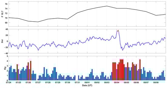
Based on the findings of statistical research on ionospheric plasma parameters associated with seismic disturbances [44,45,46,47], it has been found that anomalies predominantly arise within a two-week timeframe prior to earthquakes, with the highest frequency of anomalies occurring within the final week before the seismic event. As a consequence, our primary focus was directed towards the investigation of ionospheric disturbances 15 days before the Jiuzhaigou earthquake. Initially, several indices are employed to establish a comprehensive understanding of the pre-earthquake ionospheric spatial environment before engaging in data analysis, aiming to discern it from the effects of space weather activity on the ionosphere. Figure 1 presents the relevant indices describing the spatial weather activity from 24 July to 8 August 2017, including the solar flux at 10.7 cm (F10.7), Dst, and Kp indices. It can be seen that the solar activity was relatively calm during the study period. According to some Kp indices greater than 3 and Dst indices close to −30 nT on 24–26 July, it was indicated that there was a weak magnetic storm event. On 3–6 August, the Kp indices increased significantly, and the Dst indices showed that there was a clear onset phase of magnetic storms on 4 August with a minimum of −37 nT, and then the magnetic storm entered the recovery phase. Overall, the ionospheric spatial environment was relatively calm from 27 July to 2 August and on the days immediately before the earthquake on 7 and 8 August.
Figure 1.
Time series of F10.7, Dst, and Kp indices from 24 July to 8 August 2017. (In panel of Dst, the red line represents Dst absolute values exceeding 30 nT; in the panel of Kp, the red bar denotes indices greater than 3).
3.2. TEC Time Series Analysis of Stations near the Epicenter of the Earthquake
There exists a network of 170 monitoring stations equipped to receive GEO satellite data. Each of these stations is specifically associated with five GEO satellites, enabling the acquisition of TEC data pertaining to five IPPs. Utilizing these TEC measurements, it becomes feasible to conduct a distance-related analysis of the ionospheric TEC anomalies by calculating the distance from the epicenter to each IPP.
The interquartile range (IQR) is a parameter used to represent the dispersion of data and can be used to check for abnormalities in the data [48]. The sliding interquartile range method is often used to detect anomalies in ionospheric TEC before earthquakes [49,50]. This method can obtain a more accurate background value by calculating the median value over a period of time and determining the upper and lower limits of the ionospheric TEC based on the IQR, thereby extracting anomalies that exceed the threshold. In this study, six IPPs with more-complete data and nearest to the epicenter location are screened out. They include two IPPs of gspl, two IPPs of qhmq, and one IPP each of dlha and qhgc. In order to extract the perturbation related to the background, the sliding interquartile range method is employed to analyze the time series of TEC at each IPP, and the detailed processes are as follows.
- The median (M) and IQR of 15 days before each observation were calculated based on the preceding background. Statistically, the expected value of the interquartile range is 1.34 times the standard deviation [50,51], so disturbances were extracted using the threshold of M ± 1.5IQR.
- The calculation of abnormal values (Ab) was carried out using Equation (8), which can highlight the anomalies. Values exceeding M + 1.5IQR were considered as positive anomalies, while values below M − 1.5IQR were negative anomalies. For values exceeding the threshold, we calculated the relative change (Ab%) between the observed data (Obs) and the threshold. We assigned the value of 0 to those that do not exceed the threshold value.
- To eliminate the interference of abrupt jumps and ensure that anomalies have a certain duration, disturbances with a non-zero Ab% value persisting for over 30 min were highlighted.
In addition, the relative change amount is used in Equation (8) because there is daily variation in the TEC data. The TEC value is larger at noon so the disturbance may be easier to observe, while the changes at night are relatively small. Therefore, using relative changes avoids exaggerating perturbations in strong backgrounds and does not ignore small perturbations in weak backgrounds. This allows for more accurate analysis and detection of abnormal changes before earthquakes.
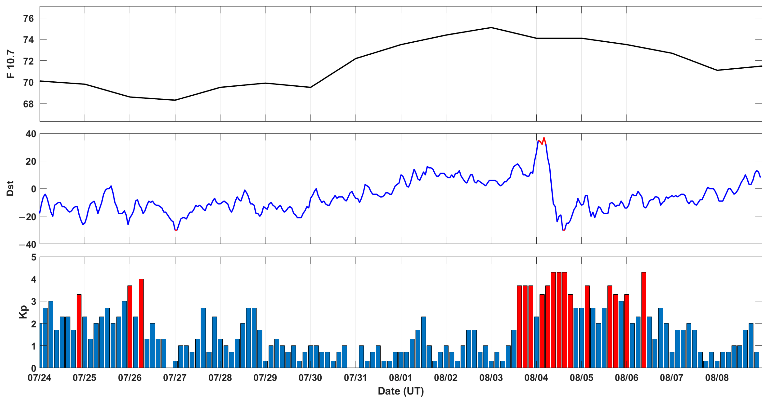
Figure 2 depicts the temporal variation of TEC in the 15 days leading up to the earthquake at the six IPPs which are closest to the epicenter and have relatively complete data. Each subgraph features the actual observed values, represented by the blue line; the upper and lower thresholds (M ± 1.5IQR), indicated by the gray lines; and anomalies with non-zero Ab% values persisting for over 30 min, shown by the red line. Based on the spatial weather background, it can be inferred that the anomalies observed from 3 August to 6 August are more likely attributed to geomagnetic storm activity. Notably, significant anomalies in terms of relative TEC temporal variations were also detected on 28 July in the relatively calm spatial weather conditions. Furthermore, exceeding threshold values were observed on 29 July, 1 August, 2 August, 7 August, and the day of the earthquake (8 August). Although these disturbances did not persist for over 30 min, they exhibited frequent fluctuations and increased diurnal amplitude, suggesting the presence of ionospheric disturbances during these periods. Colonna et al. [52] cited machine learning methods in conducting long-term observations of Italian ionospheric TEC data, and their criterion for anomaly determination is that anomalies must reoccur in a period of time. During the time period we studied, there were many recurring anomalies that lasted less than 30 min. Hence, 28 July and the periods of duration not exceeding 30 min and with a calm background environment will be the focus of the subsequent research.
Figure 2.
The time sequence change of TEC 15 days before the Jiuzhaigou Ms7.0 earthquake. (Relative TEC change curves are shown in blue lines, and upper and lower thresholds calculated by sliding interquartile range are shown in gray lines. The red curve in the bottom of each panel indicates relative change lasting more than 30 min).
3.3. Spatial and Temporal Distribution of TEC Anomalies
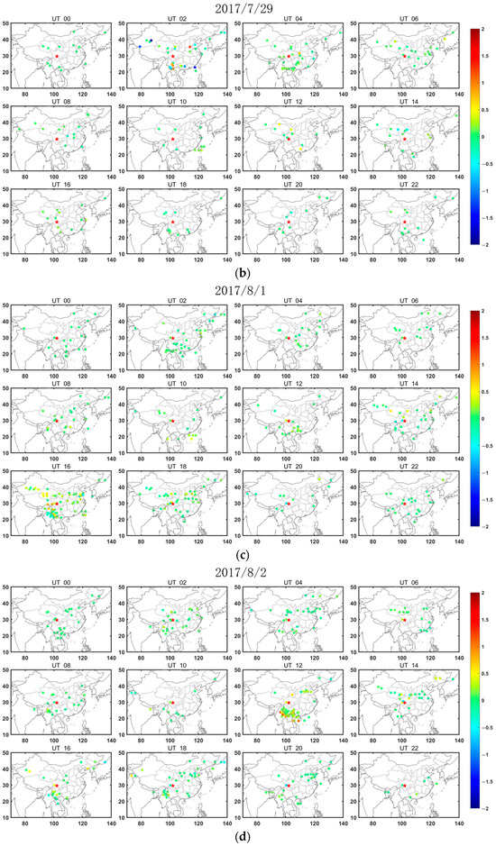
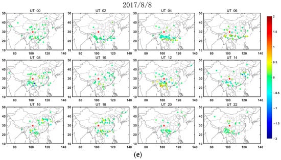
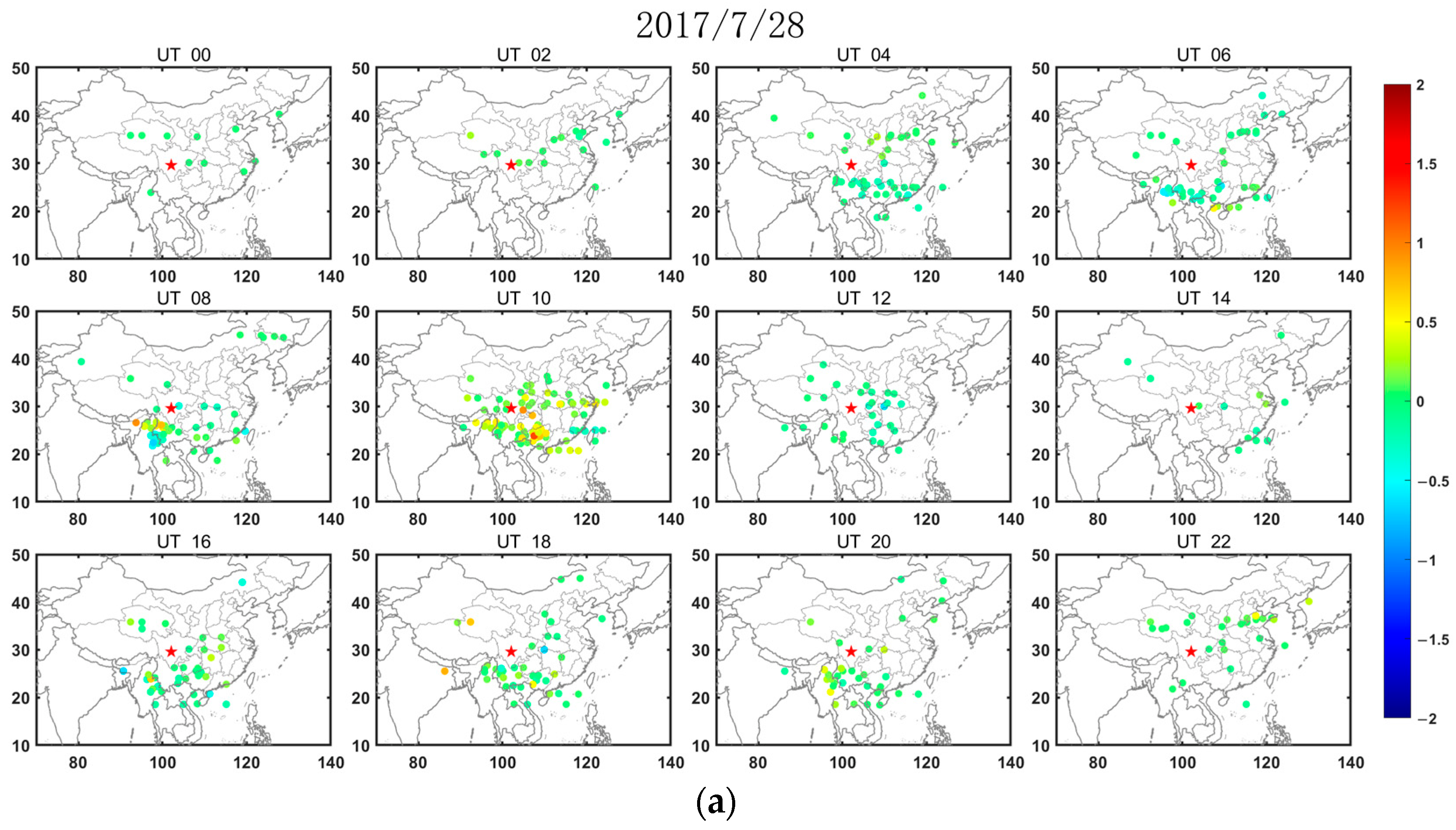
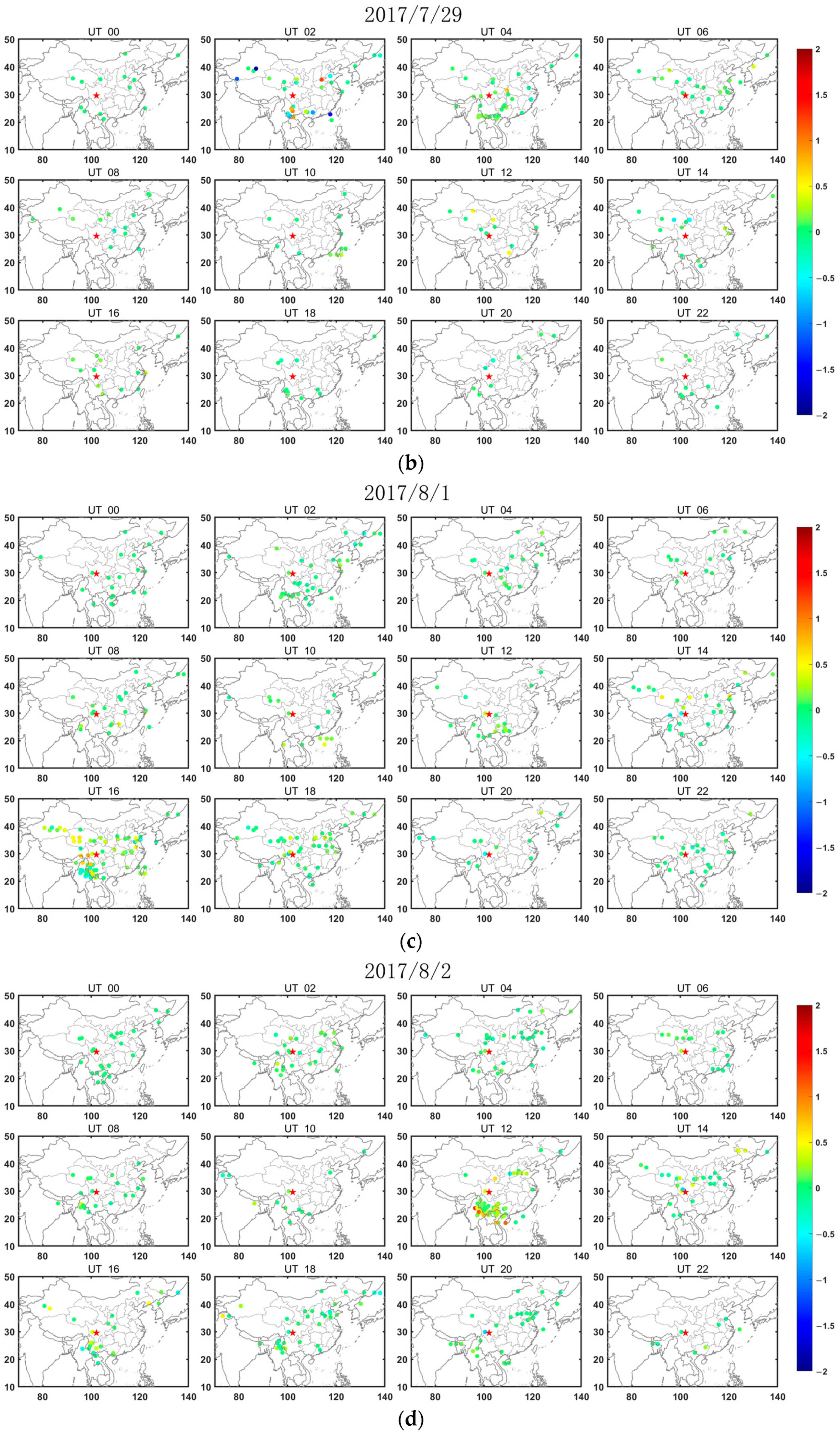
Analyzing the spatiotemporal distribution of anomalies can provide a deeper understanding of the correlation between anomaly changes and the epicenter. It allows for a more comprehensive comprehension of the spatial characteristics of ionospheric disturbances associated with earthquakes. The geostationary nature of geostationary satellites ensures that each IPP maintains a fixed position, enabling the analysis of the spatiotemporal distribution of abnormal TEC changes. Building upon the previously discussed ionospheric background environment and temporal analysis findings, we proceeded to conduct spatial and temporal analysis of TEC data during periods characterized by relatively tranquil space weather conditions. To facilitate visualization, spatial distribution maps with a temporal resolution of 2 h were generated on a daily basis. The disturbance was extracted according to the sliding interquartile range method mentioned above. For the observation data that exceeded the threshold, the difference between the observation value and the threshold is displayed at the corresponding IPP. Figure 3 shows the spatial and temporal distribution of TEC disturbances on days with significant anomalies, especially 28 July, 29 July, 1 August, 2 August, and the day of the earthquake (8 August). Compared with the temporal analysis, Figure 3 additionally shows the spatial distribution of TEC anomalies relative to the epicenter. On 28 July, negative anomalies, which were mainly concentrated on the south side of the epicenter, occurred in UT04. Positive anomalies were observed in the vicinity of the epicenter at UT08, while regions farther away continued to exhibit negative anomalies. By UT10, the positive anomaly area expanded, and subsequently, the southern side of the epicenter displayed predominantly negative anomalies. On 29 July, notable disturbances were witnessed on the southern side of the epicenter at UT02, characterized by a mixture of positive and negative anomalies. On 1 August at UT16, a significant surge in anomalies took place on the southwest side of the epicenter, primarily indicating positive anomalies. On 2 August at UT12, another noteworthy increase in anomalies occurred on the southern side of the epicenter, with the highest magnitude point located at a certain distance from the epicenter. On the day of the earthquake, 8 August, significant disturbances were observed at UT04, UT06, and UT12, along with an increased number of anomaly points. TEC decreased in the vicinity of the epicenter while it increased in the farther areas.
Figure 3.
TEC spatiotemporal distribution map. The dates of panels (a–e) are 28 July (11 days before the earthquake), 29 July (10 days before the earthquake), 1 August (7 days before the earthquake), 2 August (6 days before the earthquake), and 8 August (the day of the earthquake). (The red star represents the position of the epicentre.)
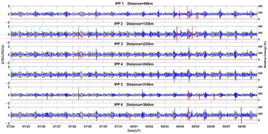
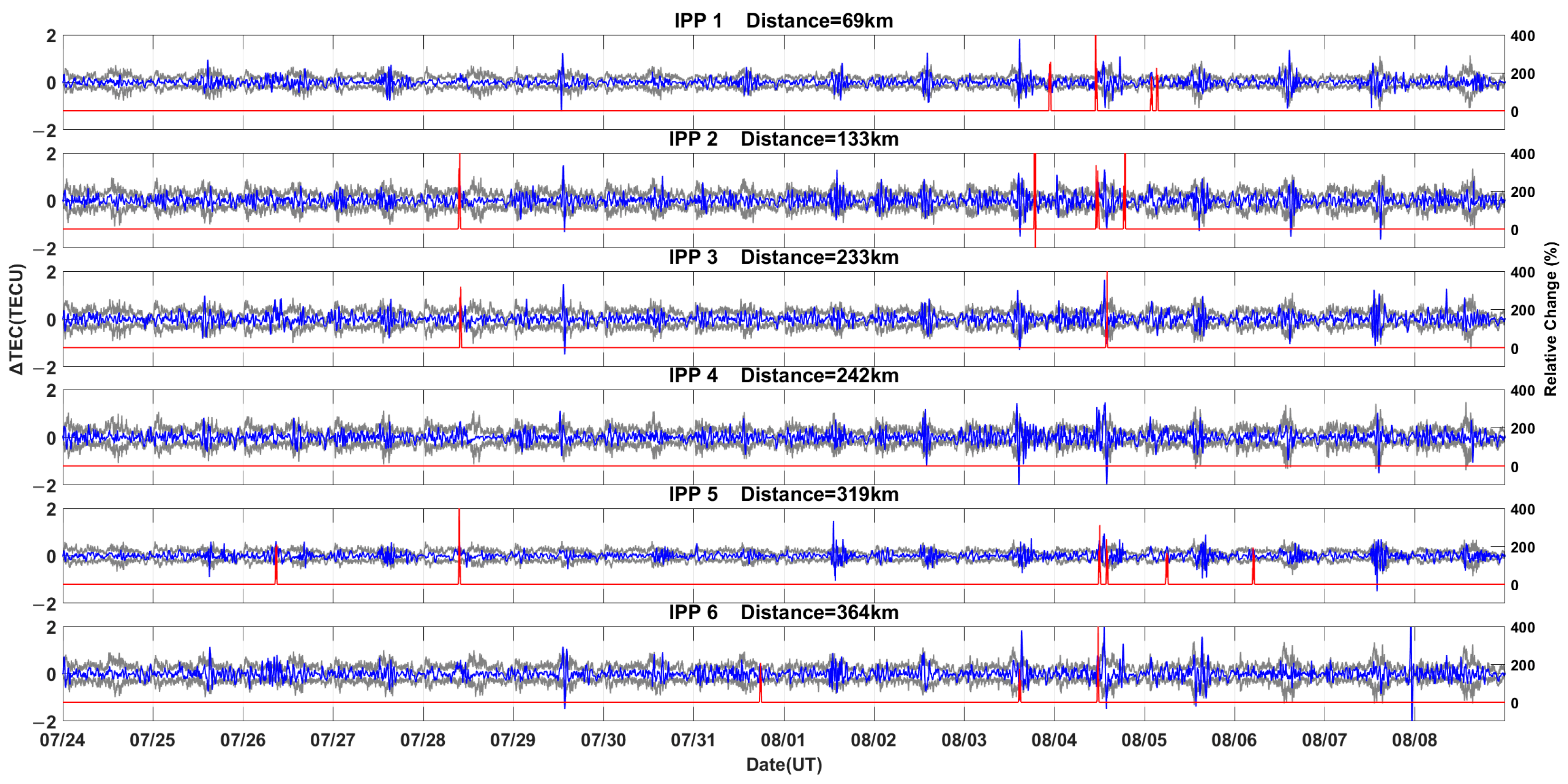
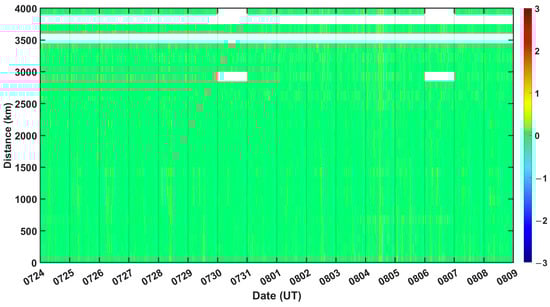
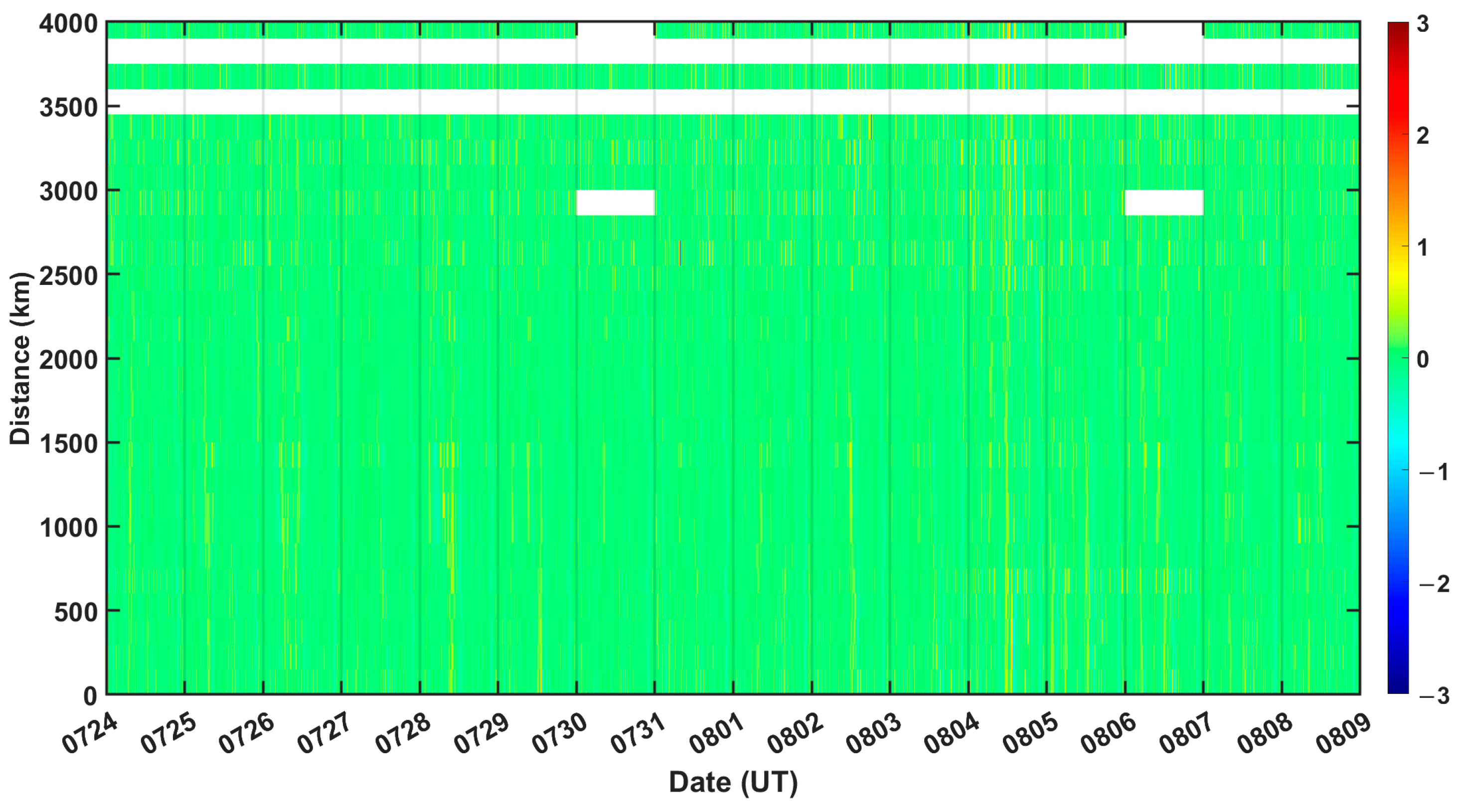
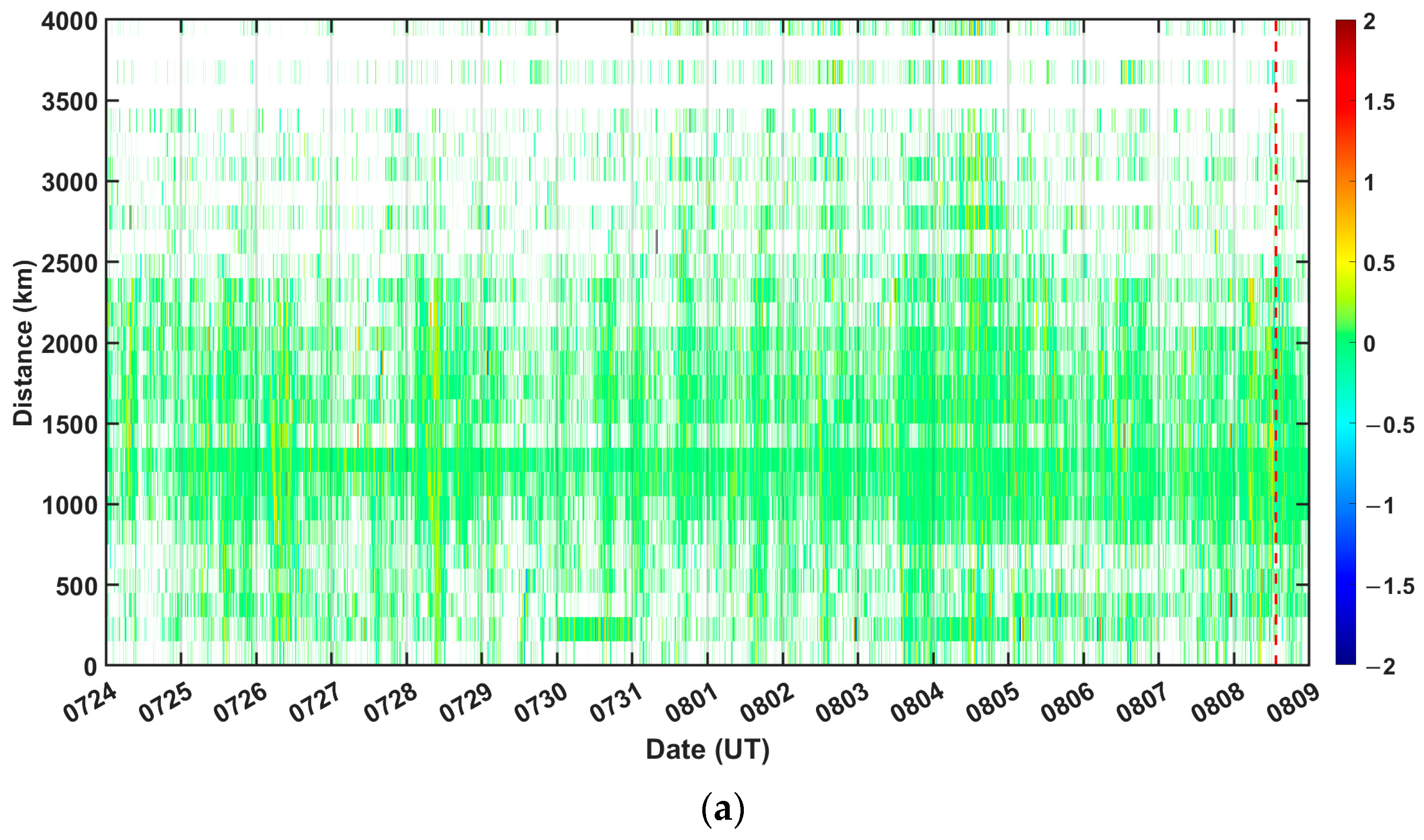
Attempting to study the spatial characteristics of TEC pre-earthquake disturbances, we further analyzed the time variation of disturbances in terms of their distance from the epicenter. The distance between each IPP and the epicenter was calculated using TEC observations taken every 30 s, which were graphed with the time and distance at a resolution of 150 km. The distribution of IPPs is uneven, which may result in the absence of data within certain distance ranges and affect the analysis results. The analysis revealed that the TEC data existed at each distance, as shown in Figure 4. By setting upper and lower thresholds as M ± 1.5IQR, the anomalous TEC data were highlighted over time and distance (Figure 5). The pictures in the abnormal days mentioned in the former illustration were enlarged and are displayed in Figure 5 for better visualization.
Figure 4.
Variation of TEC direct observations with the date (X axis) and distance from the epicenter (Y axis).
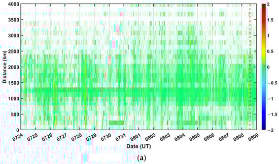
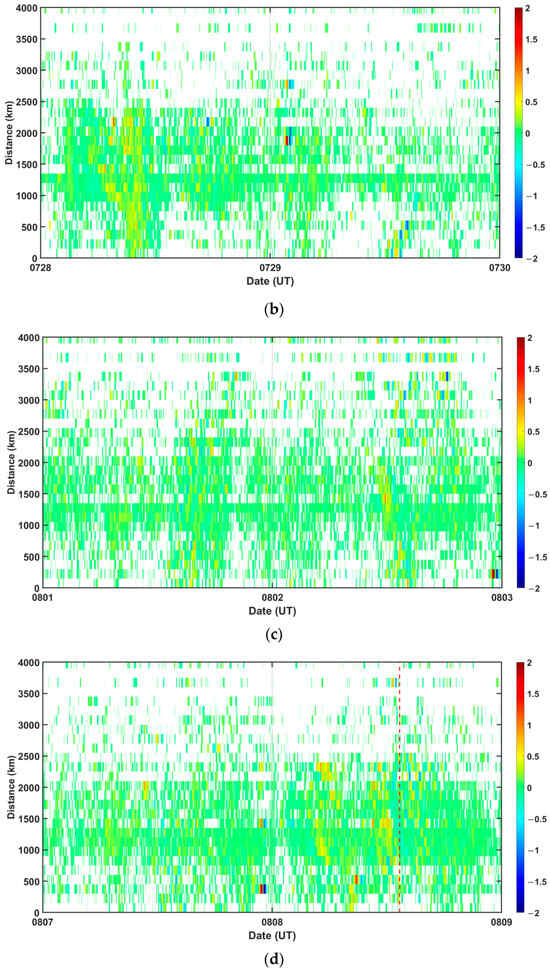
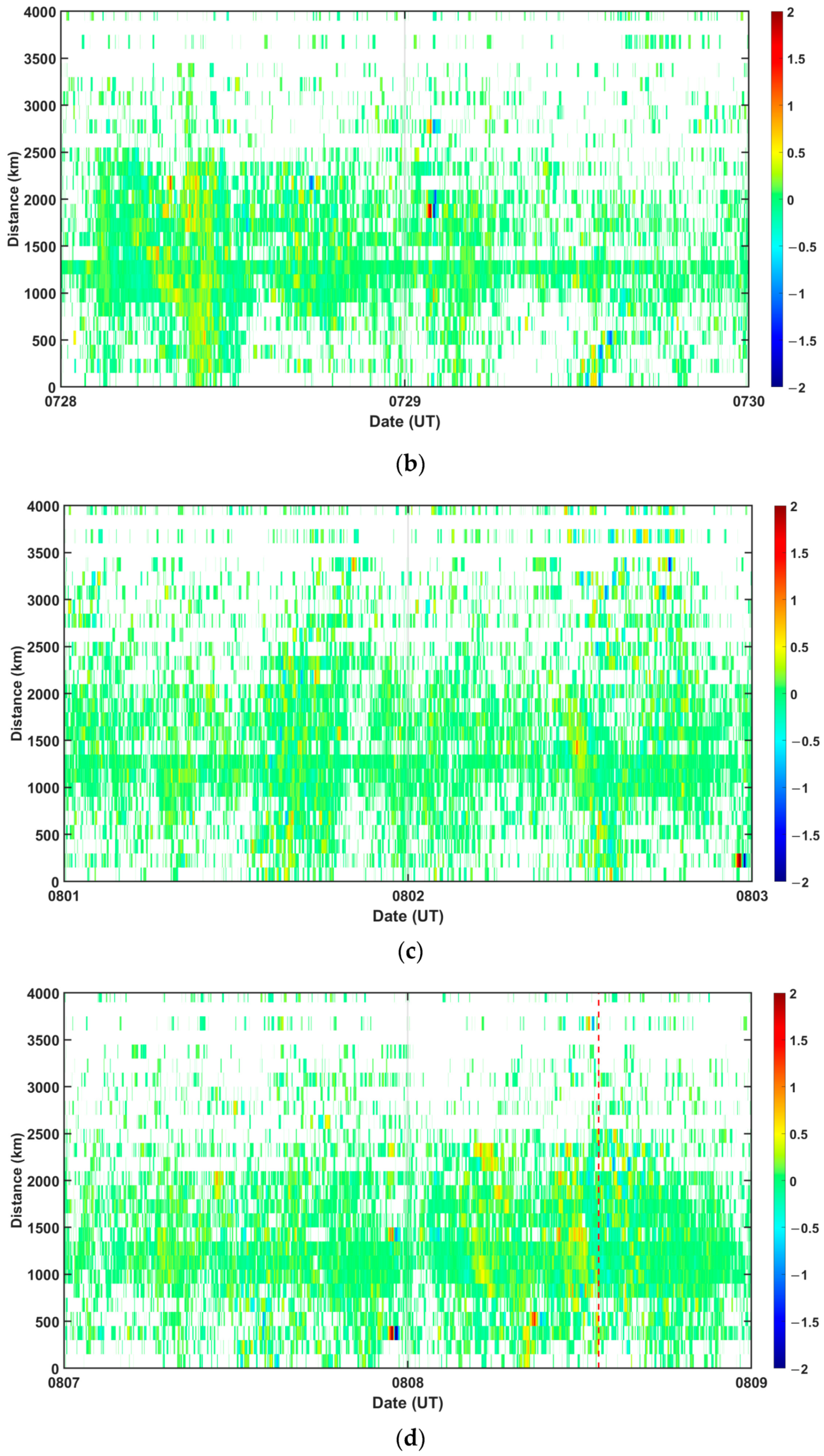
Figure 5.
TEC variation with the date (X axis) and distance from the epicenter (Y axis). The red dashed line represents the time of the earthquake. The dates of panels (a–d) are 24 July to 8 August, 28 July to 29 July, 2 August to 2 August, and 7 August to 8 August.
Corresponding to the spatiotemporal distribution results, the disturbances appeared to affect an area of nearly 2500 km on 28 July, as shown in Figure 5b. Obvious disturbance anomalies appeared within about 3000 km kilometers from the epicenter within 2–3 UT on 29 July, which were located in areas farther to the north from the spatiotemporal distribution map in Figure 3b and should have little relationship with the Jiuzhaigou earthquake. Additionally, a section of obvious TEC-lowering anomalies existed within 500 km from the epicenter at 12 UT, which gradually became farther away with time to the epicenter. Further analysis revealed that on August 1, there were obvious disturbances in different time periods from UT12 to UT18 within 2500 km from the epicenter (Figure 5c). On 2 August, the anomalies were concentrated around UT12, and the anomalies were more apparent in the area around 500 km from the epicenter. Strong positive and negative perturbations on August 7 mainly appeared around UT22, as shown in Figure 5d. The anomalies were evident from 1 to 9 h before the earthquake on 8 August, and at about 5–9 h before the quake, the anomalies gradually moved closer to the epicenter with the passage of time. In the process of studying the spatial distribution of ionospheric TEC anomalies, Sharma et al. [53] found that the distribution of TEC anomalies on the daily scale tended to move closer to the epicenter 8–9 days before the earthquake, which may be related to the stress accumulation around the fault making anomalous phenomena cluster near the epicenter. This may be the advantage of GEO’s high spatial and temporal resolution, which allows us to observe abnormal changes on an hourly scale. However, in the following 1–5 h before the quake, the anomalies showed a tendency to become farther away with time. It may be that the perturbed electric field caused by the earthquake increases the equatorial fountaining effect [54,55], which intensifies the equatorial ionization anomaly (EIA). It can be seen in the sub-panel at UT12 in Figure 3e that the northern crest of EIA is enhanced . Previous studies using GPS TEC data have detected the changes in TEC near the epicenter before the earthquake on 8 August, while they did not find this pattern of anomaly variation over time and distance around the epicenter [32,33,34,35]. Therefore, the utilization of high-resolution TEC data from BDS GEO observations is uniquely advantageous in revealing ionospheric perturbations.
4. Discussion
The generation of earthquakes is an extremely complex process that usually involves the combined effects of multiple factors. Consequently, the effects of earthquakes on the ionosphere are often multi-faceted. A model proposed by Hayakawa, namely, the LAIC model, suggests that seismic disturbance can spread from the lithosphere to the atmosphere and ionosphere via electromagnetic, acoustic, and geochemical pathways [56]. The physical processes, crustal movements, and rock ruptures that result from earthquakes may all have varying degrees of impact across different atmospheric parameters, thereby influencing the ionosphere. Additionally, a certain coupling relationship exists in different propagation paths, resulting in a multi-path coupling mechanism that further complicates the impact of earthquakes on the ionosphere. Pulinets et al. [11,12] pointed out that the release of radon gas and the propagation of acoustic waves through the chemical pathway can couple to form abnormal electric fields, which, in turn, couples with the ionosphere to produce abnormal disturbances.
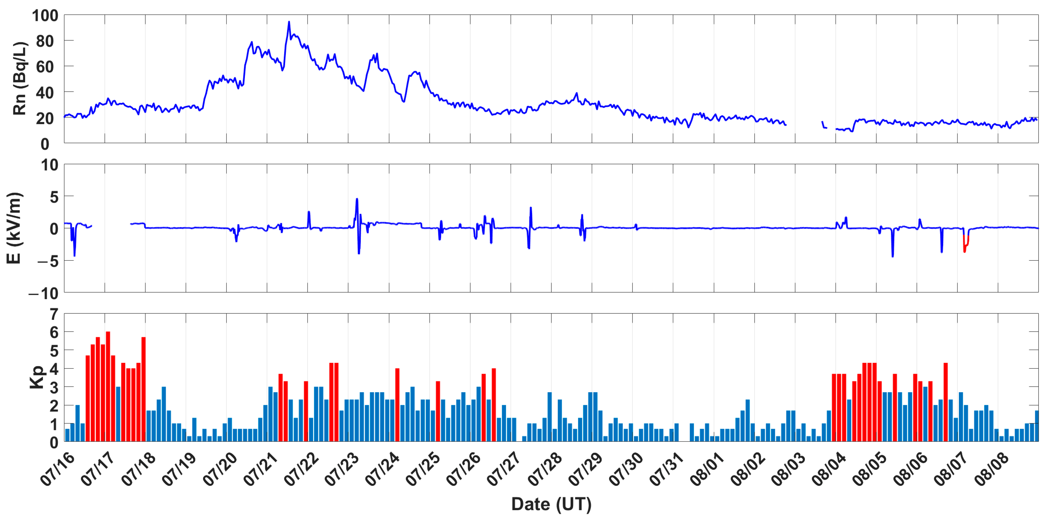
In the chemical pathway, the main factors influencing the lithosphere and near-surface atmosphere are radon gas and changes in the atmospheric electric field. Previous studies have suggested that there is a potential correlation involving heightened radon gas emissions, anomalies in atmospheric electric fields, and the incidence of earthquakes [57,58]. Therefore, the data of radon gas and the atmospheric electric field were also collected, and we sought to explore the linkage between them and the extracted ionospheric TEC disturbance. The atmospheric electric field data of Pixian station (103.9°E, 30.9°N) near the epicenter were collected from the Data Center for Meridian Space Weather Monitoring Project (https://data.meridianproject.ac.cn/, accessed on 15 September 2023), and the radon gas data of Songpan station (103.6°E, 32.7°N) were obtained from the China Earthquake Networks Center. The time series curve of the two parameters before the Jiuzhaigou earthquake are shown in Figure 6.
Figure 6.
The variation of radon gas, atmospheric electric field, and Kp from 16 July to 8 August 2017. (When the datum is below −1 kV/m and lasts for more than 2 h, it is displayed as a red curve in the temporal variation graph of the atmospheric electric field; in the panel of Kp, the red bar denotes indices greater than 3).
In order to observe the changes in radon gas, the study time range was extended sufficiently forward to observe the normal state before the accidental increase in radon gas. From 19 July to 25 July, the radon gas concentration rose, exhibited a fluctuating increase, and subsequently displayed a significant decline in the form of fluctuation, reaching its peak on 21 July. The radon gas concentration was relatively stable throughout other instances; only a slight increase was observed on 28 July. Many studies have observed that radon gas, mainly in the three weeks before an earthquake, will rise remarkably [59,60,61,62,63]. Zhou et al. [58] and Fu et al. [64] considered that the release of radon gas has a short- to medium-term impact on the ionosphere. Therefore, it is plausible to conclude that the abnormal increase in radon in Figure 6 may be related to the Jiuzhaigou earthquake.
Significant fluctuations in the atmospheric electric field were observed during three periods: 16 July, from 20–28 July, and from 4–7 August. Referring to the Kp index, it can be seen that the fluctuation changes in the atmospheric electric field are more concentrated in the range of a Kp index greater than 3. Kleimenova et al. [65] researched the changing characteristics of the atmospheric electric field during 14 magnetic storms based on observation data from mid-latitude stations. They observed that there were disturbance anomalies in the atmospheric electric field near mid-latitudes during the magnetic storms, and the disturbance range was approximately −100–150 V/m. However, disturbances also occurred on days without magnetic storms (20 July, 27 July, and 28 July). The reason for this situation may be that the atmospheric electric field is also affected by weather conditions such as thunderstorms [66], rainfall [67], and cloud cover [68]. Previous research conducted by Chen et al. [69] analyzed atmospheric electric field data obtained from a station near the epicenter prior to the Luanzhou earthquake on 16 April 2021. The authors found that the electric field observations from multiple stations showed continuous negative abnormal signals before the earthquake, and they proposed that it may be associated with impending earthquakes. Choudhury et al. [70] observed that prior to the earthquake, a bay-like variation in the magnitude of kilovolts existed in the vertical electric field. More studies have observed that the persistent negative anomalies in the magnitude of kilovolts in the atmospheric electric field occurred before earthquakes, and the authors of these studies claimed that they may be potential precursor signals of earthquakes [71,72]. Based on existing research into atmospheric electric field anomalies, we try to explain the generation mechanism of this negative abnormal signal. It has been supposed that under normal space weather conditions, a positive electric field gradient is observed due to the Earth’s surface carrying negative charges and the ionosphere carrying positive charges [71]. During the pre-seismic period, a substantial release of energy from the lithosphere to the atmosphere induces ionization, leading to the accumulation of positive ions at the Earth’s surface and subsequently resulting in negative anomalies in the electric field. Consequently, to extract an abnormality with a certain duration, the time range where the values remain below −1 kv/m for 2 h was highlighted, as shown in Figure 6. It can be seen that the continuous and negative phase disturbance in the atmospheric electric field only occurred on 7 August, one day prior to the Jiuzhaigou earthquake, which suggests a possible correlation between them.
The ionospheric disturbance resulting from the earthquake may also be linked to the acoustic–gravity waves triggered by surface motion [30,73,74,75,76]. The coupled modeling theory proposed by Pulinets implies that the pressure and density changes induced by acoustic–gravity waves could cause local ionization, resulting in anomalies in the electric field and coupling with the ionosphere [11,12]. Additionally, there exists resonance coupling among the lithosphere, atmosphere, and ionosphere, indicating that acoustic–gravity waves can influence charged particles through fluctuations, leading to changes in ionospheric TEC [30]. Huang et al. [77] investigated the interaction between the ionosphere and acoustic–gravity waves and observed that acoustic–gravity waves have the potential to cause ion accumulation in localized areas, creating plasma density gradients and ionospheric disturbances. Chen et al. [30] spectrally analyzed TEC data and noted that TEC enhancement prior to earthquakes predominantly occurs within the frequency band of 0.004–0.006 Hz. They also identified that the anomalous frequency band of acoustic–gravity waves during propagation closely aligns with the anomalous frequency band of TEC in the ionosphere, with frequencies within the range of 0.004–0.005 Hz.
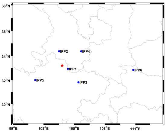
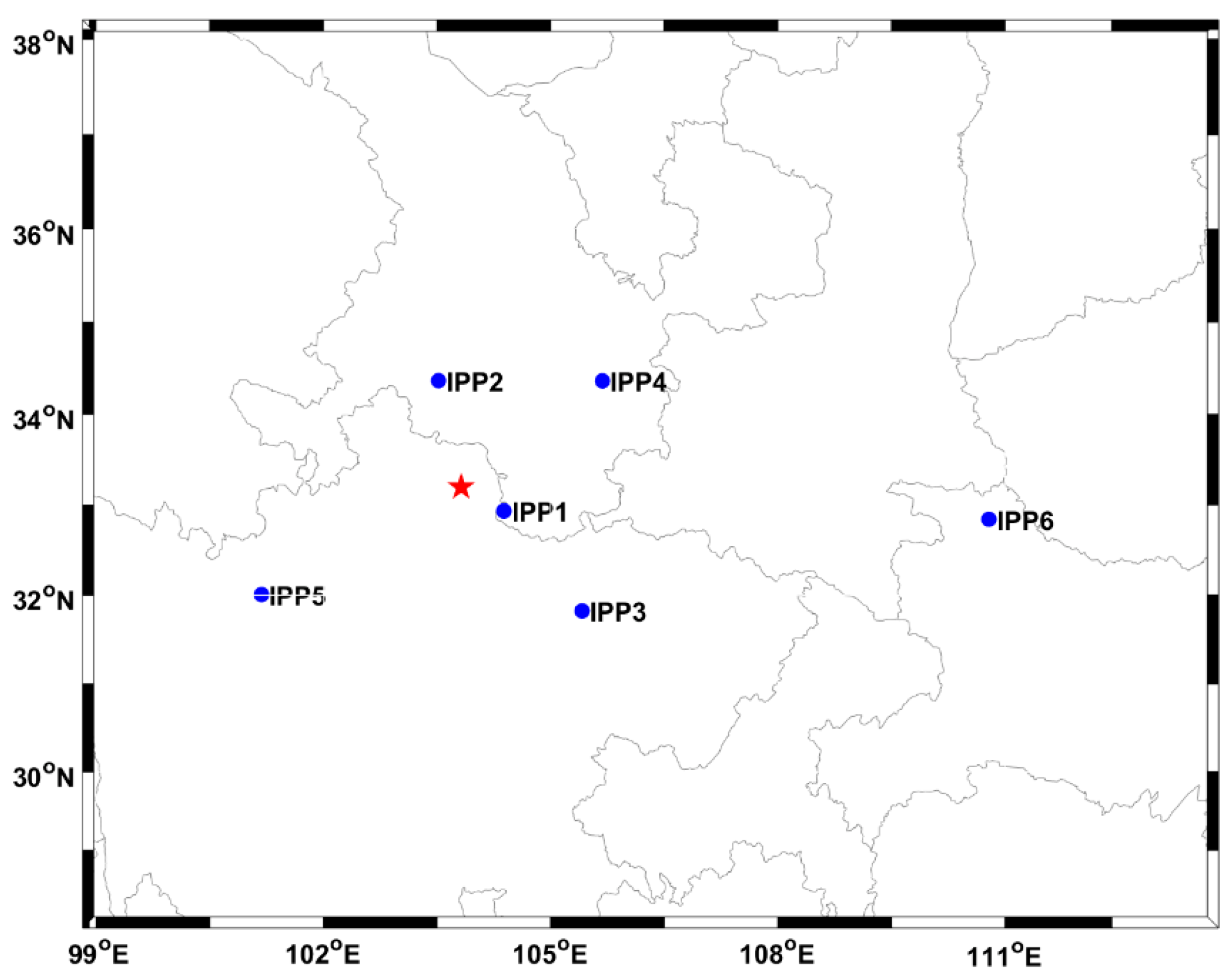
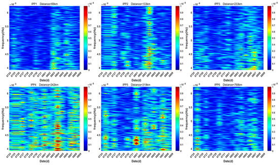
A spectral analysis of TEC data is conducted in this study to investigate the potential influence of the acoustic–gravity wave coupling pathway on ionospheric TEC changes. Initially, the data were filtered based on disturbance and epicentral distance, leading to the selection of six IPPs with complete data, anomalies, and the closest proximity to the epicenter, as depicted in Figure 7. Significantly, areas exhibiting anomalies near the epicenter were predominantly situated in the southeast and southwest directions. Subsequently, Fourier transform was performed on the time domain data of the selected IPPs, mainly examining the time changes of frequency amplitude in the frequency range of 0.004–0.006 Hz, as shown in Figure 8. During two geomagnetic storm periods, TEC exhibited overall enhancement across the frequency band, which was particularly evident in the IPP2 and IPP4 sub-figures. In relatively calm spatial periods, significant increases in TEC within the ranges of 0.004–0.0045 Hz were experienced at IPP2, IPP3, IPP5, and IPP6 on 7 August, particularly at IPP3. Observations and numerical simulations indicate that ground vibrations and ionospheric TEC share a frequency of approximately 0.004 Hz [73,74,75]. Chen et al. [41] proposed that the 0.004 Hz fluctuation in pre-earthquake TEC is likely associated with atmospheric acoustic–gravity waves generated by earthquakes. Li et al. [78] highlighted the correlation between the excitation of acoustic–gravity waves in the study area and terrain uplift, with the preferred propagation direction of acoustic–gravity waves varying based on factors such as terrain, season, and altitude. On 7 August, the locations of IPPs exhibiting amplified TEC amplitudes within the frequency range of 0.004 to 0.0045 Hz were situated in various directions from the epicenter, indicating a tendency for acoustic wave propagation outward from the epicenter. On 1 August, however, only the IPP point in the southwest direction from the epicenter demonstrated amplitude enhancement within the range of 0.004–0.0045 Hz, potentially suggesting that acoustic–gravity waves resulting from the earthquake did not propagate to other directions.
Figure 7.
Spatial distribution of the six IPPs with the closest and anomalous data. (The red star represents the position of the epicentre.)
Figure 8.
Time–frequency plots of TEC at the six IPPs in Figure 7.
From the above discussion, we preliminarily inferred that before the Ms7.0 Jiuzhaigou earthquake occurred, the radon release near the epicenter showed an increasing trend, which may potentially be the reason for the significant disturbance in the total TEC of the ionosphere on 28 and 29 July. Subsequently, acoustic–gravity waves near the epicenter propagated southwestward on 1 August, resulting in significant TEC disturbances in this direction on 1 and 2 August. Anomalies in the atmospheric electric field appeared near the epicenter on 7 August; meanwhile, the disturbances of ionospheric TEC at 0.004 to 0.0045 Hz were also detected. Under the combined influence of the anomalous electric field and the acoustic–gravity waves, the ionospheric TEC exhibited substantial superimposed anomalies from 7–8 August, as shown in Figure 5d. In the hours preceding the earthquake on 8 August, disturbances displayed a tendency to aggregate and spread to distant areas near the epicenter. This propagation trend is supposed to be associated with the stress accumulation of the fault and the amplification of EIA effected by the abnormal electric field around the epicenter. The phenomena uncovered in this investigation offer valuable insights for advancing our comprehension of the earthquake precursor phenomena, as well as the LAIC mechanism.
5. Conclusions
The analysis in this study was performed by utilizing TEC data obtained from the BeiDou GEO satellite based on CMONOC. We investigated the ionospheric disturbances preceding the Jiuzhaigou Ms7.0 earthquake in 2017 and explored the potential LAIC mechanism. Here, we summarize our main conclusions as follows:
- In the context of relatively stable solar and geomagnetic activity, ionospheric disturbances were observed near the epicenter of the Jiuzhaigou earthquake—specifically, 10 to 11 days, 6 to 7 days, and 1 to 9 h before the earthquake.
- On the spatial distribution, the anomalous TEC data prior to the earthquake were predominantly located in the southeast and southwest directions from the epicenter, with the disturbances primarily concentrated within a range of 2500 km.
- Comparing the perturbation information of radon gas, atmospheric electric field, and TEC time–frequency with the TEC perturbation in terms of time and characteristics, it was concluded that both the chemical and acoustic pathways may play important roles in the gestation process of the Jiuzhaigou Ms7.0 earthquake.
Understanding how earthquakes and ionospheric disturbances are interrelated is a complex research topic that requires a comprehensive investigation methodology, incorporating various factors and an interdisciplinary approach. In order to gain a more comprehensive understanding of the intricate relationship between earthquakes and the ionosphere, future research should concentrate on delving into the interactions between various contributing factors and determining their correlation with seismic activities. This will facilitate a more comprehensive understanding of the intricate relationship between earthquakes and the ionosphere, leading to the development of a more accurate and reliable information platform for earthquake prediction and monitoring.
The positions of IPPs detected by GPS satellites undergo changes due to the movement of these satellites. Therefore, the GPS data alone cannot directly represent the temporal variations of the TEC at specific locations in the ionosphere. To mitigate this issue, the data need to undergo mathematical interpolation or modeling techniques, coupled with high-frequency sampling, in order to minimize errors. However, BeiDou GEO satellites possess unique stationary characteristics enabling them to continuously monitor the electron content along fixed paths. As a result, BeiDou GEO satellite data can more accurately reflect the continuous variations of the ionosphere at specific locations [79]. Leveraging high-spatiotemporal-resolution data from BeiDou GEO satellites, this study unveiled the disturbance characteristics of TEC in the hours preceding an earthquake. For future research, it is anticipated that the advantages of BeiDou GEO satellite data can be fully demonstrated by analyzing more earthquake cases, contributing to a further comprehensive understanding of ionospheric disturbances triggered by earthquakes.
Author Contributions
Conceptualization, X.J., J.L. and X.Z.; methodology, X.J.; software, X.J.; validation, X.J., J.L. and X.Z.; formal analysis, X.J. and J.L.; investigation, X.J. and J.L.; resources, J.L. and X.Z.; data curation, X.J. and J.L.; writing—original draft preparation, X.J.; writing—review and editing, X.J. and J.L.; visualization, X.J.; supervision, J.L. and X.Z.; project administration, J.L. and X.Z.; funding acquisition, J.L. and X.Z. All authors have read and agreed to the published version of the manuscript.
Funding
This research was funded by the APSCO Earthquake Research Project Phase II, and ISSI-Beijing (2019-IT33).
Data Availability Statement
F10.7 index is available at the website http://www.sepc.ac.cn (accessed on 12 August 2023). Kp index is available at the website https://kp.gfz-potsdam.de/ (accessed on 12 August 2023). Dst index is available at the website https://wdc.kugi.kyoto-u.ac.jp (accessed on 12 August 2023). Atmospheric electric field data is available at the website https://data.meridianproject.ac.cn/ (accessed on 15 September 2023). The observation data of BeiDou GEO satellites are obtained from the Crustal Movement Observation Network of China (CMONOC) and radon gas data are obtained from the China Earthquake Networks Center.
Acknowledgments
The authors acknowledge Crustal Movement Observation Network of China for the observation data of BeiDou GEO satellites, the Data Center for Meridian Space Weather Monitoring Project for the atmospheric electric field data, and the China Earthquake Networks Center for the radon gas data. The authors also acknowledge the World Data Center for Geomagnetism, Kyoto for supplying Dst indices, GFZ for providing Kp index, and Space Weather Canada for supporting F10.7 index.
Conflicts of Interest
The authors declare no conflicts of interest.
References
- Chen, Y.T. Earthquake prediction: Progress, difficulties and prospect. Seismol. Geomagn. Obs. Res. 2007, 28, 1–24. [Google Scholar]
- Teng, J.W. Opportunity challenge and developing frontiers: Geophysics in 21st century. Prog. Geophys. 2004, 19, 208–215. [Google Scholar]
- Kanamori, H. Earthquake prediction: An overview. Int. Geophys. 2003, 81, 1205–1216. [Google Scholar]
- Davies, K.; Baker, D.M. Ionospheric effects observed around the time of the Alaskan earthquake of March 28, 1964. J. Geophys. Res. 1965, 70, 2251–2253. [Google Scholar] [CrossRef]
- Ding, J.H.; Shen, X.H.; Pan, W.Y.; Zhang, J.; Yu, S.R.; Li, G.; Guan, H.P. Seismo-electromagnetism precursor research progress. Chin. J. Radio Sci. 2006, 21, 791–801. [Google Scholar]
- Le, H.J.; Liu, J.; Zhao, B.Q.; Liu, L.B. Recent progress in ionospheric earthquake precursor study in China: A brief review. J. Asian Earth Sci. 2015, 114, 420–430. [Google Scholar] [CrossRef]
- Cai, J.T.; Zhao, G.Z.; Zhan, Y.; Tang, J.; Chen, X.B. The study on ionospheric disturbances during earthquakes. Prog. Geophys. 2007, 22, 695–701. [Google Scholar]
- Li, J.Z.; Wang, L.H. Analysis of daily geomagnetic variation anomalies before the Jiuzhaigou 7.0, Jinghe 6.6, and Aksu 5.7 earthquakes. Recent Dev. World Seismol. 2019, 08, 152–153. [Google Scholar]
- Nayak, K.; Romero-Andrade, R.; Sharma, G.; Zavala, J.L.C.; Urias, C.L.; Trejo Soto, M.E.; Aggarwal, S.P. A combined approach using b-value and ionospheric GPS-TEC for large earthquake precursor detection: A case study for the Colima earthquake of 7.7 Mw, Mexico. Acta Geod. Geophys. 2023, 58, 515–538. [Google Scholar] [CrossRef]
- Ruan, Q.; Yuan, X.; Liu, H.; Ge, S. Study on co-seismic ionospheric disturbance of Alaska earthquake on July 29, 2021 based on GPS TEC. Sci. Rep. 2023, 13, 10679. [Google Scholar] [CrossRef]
- Pulinets, S.; Boyarchuk, K. Ionospheric Precursors of Earthquakes; Springer: Berlin/Heidelberg, Germany, 2004. [Google Scholar]
- Pulinets, S.; Ouzounov, D. Lithosphere–Atmosphere–Ionosphere Coupling (LAIC) model—An unified concept for earthquake precursors validation. J. Asian Earth Sci. 2011, 41, 371–382. [Google Scholar] [CrossRef]
- Zhang, X.M.; Shen, X.H. The development in seismo-ionospheric coupling mechanism. Prog. Earthq. Sci. 2022, 52, 193–202. [Google Scholar]
- Liu, J.Y.; Chuo, Y.J.; Shan, S.J.; Tsai, Y.B.; Chen, Y.I.; Pulinets, S.A.; Yu, S.B. Pre-earthquake ionospheric anomalies registered by continuous GPS TEC measurements. Ann. Geophys. 2004, 22, 1585–1593. [Google Scholar] [CrossRef]
- Singh, O.P.; Chauhan, V.; Singh, V.; Singh, B. Anomalous variation in total electron content (TEC) associated with earthquakes in India during September 2006–November 2007. Phys. Chem. Earth Parts A/B/C 2009, 34, 479–484. [Google Scholar] [CrossRef]
- Shah, M.; Aibar, A.C.; Tariq, M.A.; Ahmed, J.; Ahmed, A. Possible ionosphere and atmosphere precursory analysis related to Mw > 6.0 earthquakes in Japan. Remote Sens. Environ. 2020, 239, 1–9. [Google Scholar] [CrossRef]
- Shah, M.; Jin, S. Pre-seismic ionospheric anomalies of the 2013 Mw = 7.7 Pakistan earthquake from GPS and COSMIC observations. Geod. Geodyn. 2018, 9, 378–387. [Google Scholar] [CrossRef]
- Tariq, M.A.; Shah, M.; Hernández-Pajares, M.; Iqbal, T. Pre-earthquake ionospheric anomalies before three major earthquakes by GPS-TEC and GIM-TEC data during 2015–2017. Adv. Space Res. 2019, 63, 2088–2099. [Google Scholar] [CrossRef]
- Ghimire, B.D.; Chapagain, N.P. Ionospheric Anomalies due to Nepal Earthquake-2015 as Observed from GPS-TEC Data. Geomagn. Aeron. 2022, 62, 460–473. [Google Scholar] [CrossRef]
- Takahashi, H.; Wrasse, C.M.; Denardini, C.M.; Pádua, M.B.; De Paula, E.R.; Costa, S.M.A.; Otsuka, Y.; Shiokawa, K.; Monico, J.F.G.; Ivo, A.; et al. Ionospheric TEC Weather Map over South America. Space Weather 2016, 14, 937–949. [Google Scholar] [CrossRef]
- Nayak, K.; López-Urías, C.; Romero-Andrade, R.; Sharma, G.; Guzmán-Acevedo, G.M.; Trejo-Soto, M.E. Ionospheric Total Electron Content (TEC) Anomalies as Earthquake Precursors: Unveiling the Geophysical Connection Leading to the 2023 Moroccan 6.8 Mw Earthquake. Geosciences 2023, 13, 319. [Google Scholar] [CrossRef]
- Wang, Z.; Xue, K.; Wang, C.; Zhang, T.; Fan, L.; Hu, Z.; Shi, C.; Jing, G. Near real-time modeling of global ionospheric vertical total electron content using hourly IGS data. Chin. J. Aeronaut. 2021, 34, 386–395. [Google Scholar] [CrossRef]
- Chen, X.L.; Li, S.L.; Liu, J.; Liu, Z.M. An Earthquake Emergency Command System Based on BeiDou Satellite Communication. China Earthq. Eng. J. 2020, 42, 1465–1472. [Google Scholar]
- Yang, Y.X. Progress Contribution and Challenges of Compass/Beidou Satellite Navigation System. Acta Geod. Cartogr. Sin. 2010, 39, 1–6. [Google Scholar]
- Wang, Z.J. Ionospheric Disturbance Based on Beidou Satellite Signal in Guilin. Master’s Thesis, Wuhan University, Wuhan, China, 2021. [Google Scholar]
- Ning, Z.H. Research on Ionospheric Monitoring Technology Based on Beidou Satellite Data. Master’s Thesis, Civil Aviation University of China, Tianjin, China, 2022. [Google Scholar]
- Wu, X.L.; Han, C.H.; Ping, J.S. Monitoring and analysis of regional ionosphere with GEO satellite observations. Acta Geod. Cartogr. Sin. 2013, 42, 13–18. [Google Scholar]
- Tang, J.; Gao, X.; Li, Y.J.; Zhong, Z.Y. Spatial-temporal variations of the ionospheric TEC during the August 2018 geomagnetic storm by BeiDou GEO Satellites. Acta Geod. Cartogr. Sin. 2022, 51, 317–326. [Google Scholar]
- Ming, F.X.; Ma, J.S. Study on Ionospheric Anomaly during Geomagnetic Storm by Beidou GEO Satellites. Geospat. Inf. 2023, 21, 100–103. [Google Scholar]
- Chen, C.H.; Sun, Y.Y.; Xu, R.; Lin, K.; Wang, F.; Zhang, D.X.; Zhou, Y.L.; Gao, Y.X.; Zhang, X.M.; Yu, H.Z.; et al. Resident Waves in the Ionosphere before the M6.1 Dali and M7.3 Qinghai Earthquakes of 21–22 May 2021. Earth Space Sci. 2022, 9, 1–7. [Google Scholar] [CrossRef]
- Wang, F.; Zhang, X.M.; Dong, L.; Liu, J.; Mao, Z.Q.; Lin, K.; Chen, C.-H. Monitoring Seismo-TEC Perturbations Utilizing the Beidou Geostationary Satellites. Remote Sens. 2023, 15, 2608. [Google Scholar] [CrossRef]
- Zhang, M.M.; Liu, Z.M.; Liu, P.; Cong, J.F. Analysis of ionospheric TEC anomlies before the Jiuzhaigou Ms7.0 earthquake. Eng. Surv. Mapp. 2018, 27, 24–30. [Google Scholar]
- Liu, J.; Chen, C.; He, F.X. Analysis of Ionospheric Nomalies before Wenchuan and Jiuzhaigou Earthquakes based on GPS data. Earthq. Res. Sichuan 2019, 04, 11–15+20. [Google Scholar]
- Xu, Y.L.; Wei, Q.; Tian, Y.D. Analysis of Ionospheric TEC Anomaly before M7.0 Earthquake in Jiuzhaigou. Stand. Surv. Mapp. 2021, 37, 50–53. [Google Scholar]
- Yang, J.; Zhang, Y.; Hu, L.C.; Wang, L.W.; Zhu, F.Y. Impending Ionospheric Anomalies before the 2017 Jiuzhaigou M7.0 Earthquake. Earthquake 2022, 42, 100–110. [Google Scholar]
- Zhu, J.T.; Zhao, M.X.; Gong, C.F.; Wang, L. Ionosphere abnormalities before the 2017 MS 7. 0 Jiuzhai Valley earthquake. J. Guilin Univ. Technol. 2020, 40, 372–378. [Google Scholar]
- Wen, J.; Wang, D.M.; Meng, Y.Y.; Fang, H.B. Application of BEIDOU navigation satellite system to geological survey. J. Geomech. 2012, 18, 213–223. [Google Scholar]
- Liu, J.Y. Status and Development of the Beidou Navigation Satellite System. J. Telem. Track Command. 2013, 34, 1–8. [Google Scholar]
- Bao, R. Performance Comparison of BeiDou Satellite Navigation System and Global Positioning System. Inf. Commun. 2013, 07, 3–4. [Google Scholar]
- Steigenberger, P.; Hugentobler, U.; Hauschild, A.; Montenbruck, O. Orbit and clock analysis of Compass GEO and IGSO satellites. J. Geod. 2013, 87, 515–525. [Google Scholar] [CrossRef]
- Gong, Y.Z.; Cai, C.S. A Calculation Method of Ionospheric TEC Using Triple-Frequency GNSS Observations. J. Geod. Geodyn. 2017, 37, 205–208+214. [Google Scholar]
- Wang, J.; He, H.M.; Dong, W.B. Analysis of ionospheric change characteristics based on Beidou satellites. Hous. Real Estate 2021, 15, 244–246. [Google Scholar]
- Wang, Q.; Zhu, J. Characteristic Analysis of the Differences between TEC Values in GIM Grids. Ann. Geophys. 2023, 25, 1–15. [Google Scholar]
- Liu, J.Y.; Chen, Y.I.; Jhuang, H.K.; Lin, Y.H. Ionospheric foF2 and TEC Anomalous Days Associated with M >= 5.0 Earthquakes in Taiwan during 1997–1999. Terr. Atmos. Ocean. Sci. 2004, 15, 371–383. [Google Scholar] [CrossRef]
- Ryu, K.; Lee, E.; Chae, J.S.; Parrot, M.; Pulinets, S. Seismo-ionospheric coupling appearing as equatorial electron density enhancements observed via DEMETER electron density measurements. J. Geophys. Res. Space Phys. 2014, 119, 8524–8542. [Google Scholar] [CrossRef]
- Li, M.; Shen, X.H.; Parrot, M.; Zhang, X.M.; Zhang, Y.; Yu, C.; Yan, R.; Liu, D.P.; Lu, H.X.; Guo, F.; et al. Primary Joint Statistical Seismic Influence on Ionospheric Parameters Recorded by the CSES and DEMETER Satellites. J. Geophys. Res. Space Phys. 2020, 125, 1–13. [Google Scholar] [CrossRef]
- Song, R.; Hattori, K.; Zhang, X.M.; Sanaka, S. Seismic-ionospheric effects prior to four earthquakes in Indonesia detected by the China seismo-electromagnetic satellite. J. Atmos. Sol.-Terr. Phys. 2020, 205, 1–20. [Google Scholar] [CrossRef]
- Yao, L.; Shen, X.H.; Zhang, X.M. Analysis of Ionospheric Anomalies Preceding the 2010 Yushu Ms7.1 Earthquake. Earthquake 2014, 34, 74–85. [Google Scholar]
- Chen, D.; Meng, D.; Wang, F.; Gou, Y. A study of ionospheric anomaly detection before the August 14, 2021 Mw7.2 earthquake in Haiti based on sliding interquartile range method. Acta Geod. Geophys. 2023, 58, 539–551. [Google Scholar] [CrossRef]
- Yang, K.K.; Liu, L.L.; Chen, J. Abnormality of ionospheric TEC during earthquake based on sliding interquartile rang method. J. Guilin Univ. Technol. 2019, 39, 427–432. [Google Scholar]
- Liu, J.Y.; Chen, Y.I.; Chen, C.H.; Liu, C.Y.; Chen, C.Y.; Nishihashi, M.; Li, J.Z.; Xia, Y.Q.; Oyama, K.I.; Hattori, K.; et al. Seismoionospheric GPS total electron content anomalies observed before the 12 May 2008 Mw7.9 Wenchuan earthquake. J. Geophys. Res. Space Phys. 2009, 114, 1–10. [Google Scholar] [CrossRef]
- Colonna, R.; Filizzola, C.; Genzano, N.; Lisi, M.; Tramutoli, V. Optimal Setting of Earthquake-Related Ionospheric TEC (Total Electron Content) Anomalies Detection Methods: Long-Term Validation over the Italian Region. Geosciences 2023, 13, 150. [Google Scholar] [CrossRef]
- Sharma, G.; Romero-Andrade, R.; Taloor, A.K.; Ganeshan, G.; Sarma, K.K.; Aggarwal, S.P. 2-D ionosphere TEC anomaly before January 28, 2020, Cuba earthquake observed from a network of GPS observations data. Arab. J. Geosci. 2022, 15, 1–11. [Google Scholar] [CrossRef]
- Pulinets, S.A.; Legen’ka, A.D. Dynamics of the near-equatorial ionosphere prior to strong earthquakes. Geomagn. Aeron. 2002, 42, 227–232. [Google Scholar]
- Pulinets, S. Low-Latitude Atmosphere-Ionosphere Effects Initiated by Strong Earthquakes Preparation Process. Int. J. Geophys. 2012, 2012, 1–14. [Google Scholar] [CrossRef]
- Hayakawa, M. Electromagnetic Phenomena Associated with Earthquakes. IEEJ Trans. Fundam. Mater. 2006, 126, 211–214. [Google Scholar] [CrossRef]
- Smirnov, S. Negative Anomalies of the Earth’s Electric Field as Earthquake Precursors. Geosciences 2020, 10, 10. [Google Scholar] [CrossRef]
- Zhou, H.; Su, H.; Li, C.; Wan, Y. Geochemical precursory characteristics of soil gas Rn, Hg, H2, and CO2 related to the 2019 Xiahe Ms5.7 earthquake across the northern margin of West Qinling fault zone, Central China. J. Environ. Radioact. 2023, 264, 107190. [Google Scholar] [CrossRef] [PubMed]
- Ui, H.; Moriuchi, H.; Takemura, Y.; Tsuchida, H.; Fujii, I.; Nakamura, M. Anomalously high radon discharge from the atotsugawa fault prior to the western nagano prefecture earthquake (m 6.8) of September 14, 1984. Tectonophysics 1988, 152, 147–152. [Google Scholar] [CrossRef]
- Igarashi, G.; Saeki, S.; Takahata, N.; Sumikawa, K.; Tasaka, S.; Sasaki, Y.; Takahashi, M.; Sano, Y. Ground-water radon anomaly before the kobe earthquake in Japan. Science 1995, 269, 60–61. [Google Scholar] [CrossRef] [PubMed]
- Li, C.; Su, H.; Zhang, H.; Zhou, H. Correlation between the spatial distribution of radon anomalies and fault activity in the northern margin of West Qinling Fault Zone, Central China. J. Radioanal. Nucl. Chem. 2015, 308, 679–686. [Google Scholar] [CrossRef]
- Fu, C.-C.; Walia, V.; Yang, T.F.; Lee, L.-C.; Liu, T.-K.; Chen, C.-H.; Kumar, A.; Lin, S.-J.; Lai, T.-H.; Wen, K.-L. Preseismic anomalies in soil-gas radon associated with 2016 M 6.6 Meinong earthquake, Southern Taiwan. Terr. Atmos. Ocean. Sci. 2017, 28, 787–798. [Google Scholar] [CrossRef]
- Soldati, G.; Cannelli, V.; Piersanti, A. Monitoring soil radon during the 2016–2017 central Italy sequence in light of seismicity. Sci. Rep. 2020, 10, 13137. [Google Scholar] [CrossRef] [PubMed]
- Fu, C.C.; Yang, T.F.; Tsai, M.C.; Lee, L.C.; Liu, T.K.; Walia, V.; Chen, C.H.; Chang, W.Y.; Kumar, A.; Lai, T.H. Exploring the relationship between soil degassing and seismic activity by continuous radon monitoring in the Longitudinal Valley of eastern Taiwan. Chem. Geol. 2017, 469, 163–175. [Google Scholar] [CrossRef]
- Kleimenova, N.; Kozyreva, O.; Michnowski, S.; Kubicki, M. Influence of geomagnetic disturbances on atmospheric electric field (Ez) variations at high and middle latitudes. J. Atmos. Sol.-Terr. Phys. 2013, 99, 117–122. [Google Scholar] [CrossRef]
- Liu, C.; Williams, E.R.; Zipser, E.J.; Burns, G. Diurnal Variations of Global Thunderstorms and Electrified Shower Clouds and Their Contribution to the Global Electrical Circuit. J. Atmos. Sci. 2010, 67, 309–323. [Google Scholar] [CrossRef]
- Telang, A.V.R. The influence of rain on the atmospheric-electric field. Terr. Magn. Atmos. Electr. 1930, 35, 125–131. [Google Scholar] [CrossRef]
- Tinsley, B.A.; Burns, G.B.; Zhou, L. The role of the global electric circuit in solar and internal forcing of clouds and climate. Adv. Space Res. 2007, 40, 1126–1139. [Google Scholar] [CrossRef]
- Chen, T.; Wang, S.H.; Li, L.; Yang, M.P.; Zhang, L.Q.; Zhang, X.M.; Huang, F.Q.; Liu, J.; Xiong, P.; Ti, S.; et al. Analysis of the Abnormal Signal of Atmospheric Electric Feild before the Luanzhou Ms4.3 Earthquake on April 16,2021. J. Geod. Geodyn. 2022, 42, 771–776. [Google Scholar]
- Abhijit, C.; Anirban, G.; Barin Kumar, D.; Rakesh, R. A statistical study on precursory effects of earthquakes observed through the atmospheric vertical electric field in northeast India. Ann. Geophys. 2013, 56, R0331. [Google Scholar]
- Chen, T.; Zhang, X.X.; Zhang, X.M.; Jin, X.B.; Wu, H.; Ti, S.; Li, R.K.; Li, L.; Wang, S.H. Imminent estimation of earthquake hazard by regional network monitoring the near surface vertical atmospheric electrostatic field. Chin. J. Geophys. 2021, 64, 1145–1154. [Google Scholar]
- Smirnov, S. Earth electric field negative anomalies as earthquake precursors. E3S Web Conf. 2020, 196, 1–6. [Google Scholar] [CrossRef]
- Dautermann, T.; Calais, E.; Lognonn, P.; Mattioli, G.S. Lithosphere-atmosphere-ionosphere coupling after the 2003 explosive eruption of the Soufriere Hills Volcano, Montserrat. Geophys. J. Int. 2009, 179, 1537–1546. [Google Scholar] [CrossRef]
- Chen, C.H.; Saito, A.; Lin, C.H.; Liu, J.Y.; Tsai, H.F.; Tsugawa, T.; Otsuka, Y.; Nishioka, M.; Matsumura, M. Long-distance propagation of ionospheric disturbance generated by the 2011 off the Pacific coast of Tohoku Earthquake. Earth Planets Space 2011, 63, 881–884. [Google Scholar] [CrossRef]
- Liu, J.Y.; Chen, C.H.; Lin, C.H.; Tsai, H.F.; Chen, C.H.; Kamogawa, M. Ionospheric disturbances triggered by the 11 March 2011M9.0 Tohoku earthquake. J. Geophys. Res. Space Phys. 2011, 116, 1–5. [Google Scholar] [CrossRef]
- Chou, M.Y.; Cherniak, I.; Lin, C.C.H.; Pedatella, N.M. The Persistent Ionospheric Responses Over Japan after the Impact of the 2011 Tohoku Earthquake. Space Weather 2020, 18, 1–22. [Google Scholar] [CrossRef]
- Huang, C.S.; Li, J. Nonlinear ionospheric response to the atmospheric gravity waves. Astron. Res. Technol. 1990, S1, 44–48. [Google Scholar]
- Li, J.; Li, L.B.; Wu, Z.H.; Wan, W.X.; Ning, B.Q. ionospheric disturbances related to the meteorology of Qinghai-Xizang plateau. Astron. Res. Technol. 1990, S1, 1–6. [Google Scholar]
- Kunitsyn, V.; Kurbatov, G.; Yasyukevich, Y.; Padokhin, A. Investigation of SBAS L1/L5 Signals and Their Application to the Ionospheric TEC Studies. IEEE Geosci. Remote Sens. Lett. 2015, 12, 547–551. [Google Scholar] [CrossRef]


Disclaimer/Publisher’s Note: The statements, opinions and data contained in all publications are solely those of the individual author(s) and contributor(s) and not of MDPI and/or the editor(s). MDPI and/or the editor(s) disclaim responsibility for any injury to people or property resulting from any ideas, methods, instructions or products referred to in the content. |
© 2024 by the authors. Licensee MDPI, Basel, Switzerland. This article is an open access article distributed under the terms and conditions of the Creative Commons Attribution (CC BY) license (https://creativecommons.org/licenses/by/4.0/).