Article

Airborne Hyperspectral Images and Machine Learning Algorithms for the Identification of Lupine Invasive Species in Natura 2000 Meadows

Department of Geoinformatics, Cartography and Remote Sensing, Faculty of Geography and Regional Studies, University of Warsaw, ul. Krakowskie Przedmieście 30, 00-927 Warsaw, Poland
*
Author to whom correspondence should be addressed.
Remote Sens. 2024, 16(3), 580; https://doi.org/10.3390/rs16030580
Submission received: 18 November 2023 / Revised: 24 January 2024 / Accepted: 1 February 2024 / Published: 3 February 2024

Abstract

:
The mapping of invasive plant species is essential for effective ecosystem control and planning, especially in protected areas. One of the widespread invasive plants that threatens the species richness of Natura 2000 habitats in Europe is the large-leaved lupine (Lupinus polyphyllus). In our study, this species was identified at two Natura 2000 sites in southern Poland using airborne HySpex hyperspectral images, and support vector machine (SVM) and random forest (RF) classifiers. Aerial and field campaigns were conducted three times during the 2016 growing season (May, August, and September). An iterative accuracy assessment was performed, and the influence of the number of minimum noise fraction (MNF) bands on the obtained accuracy of lupine identification was analyzed. The highest accuracies were obtained for the August campaign using 30 MNF bands as input data (median F1 score for lupine was 0.82–0.85), with lower accuracies for the May (F1 score: 0.77–0.81) and September (F1 score: 0.78–0.80) campaigns. The use of more than 30 MNF bands did not significantly increase the classification accuracy. The SVM and RF algorithms allowed us to obtain comparable results in both research areas (OA: 89–94%). The method of the multiple classification and thresholding of frequency images allowed the results of many predictions to be included in the final map.

1. Introduction

Invasive alien plant species (IAS), exceeding the biogeographic borders of their natural habitats [1,2], destroy natural ecosystems and cause ecological and economic dysfunction [3,4,5]. Therefore, it is crucial to prevent the further spread of IAS, especially in Natura 2000 sites, established to ensure the long-term sustainability of valuable species and habitats in Europe. One of the widespread invasive species that threatens the biological richness of mountain meadows and grasslands is Lupinus polyphyllus Lindl., also known as garden lupin or large-leaved lupine. By creating dense patches and producing allelopathic substances, this species may limit the germination of native plants and be harmful to farm animals, which is why it was chosen as the subject of this study [6,7].
Remote sensing and machine learning methods have been increasingly used for monitoring the spread of invasive species [8,9]. Currently, various types of remote sensing imagery are available, and their selection involves a compromise between spatial, spectral, and temporal resolution and the spatial extent of the image [8,10]. Satellite data have been successfully used to identify invasive trees, shrubs, and tall perennials [11,12]. However, to detect herbaceous plants in the initial phases of invasion, it is helpful to use data with higher spatial resolution from airplanes or unmanned aerial vehicles (UAVs, [13,14]), but such analyses are oriented toward local case studies. Hyperspectral data are useful for morphologically similar plants [15,16,17] due to the identification of unique spectral signatures of plant species [18]. The use of HySpex hyperspectral data has enabled the accurate identification of wild cucumber (Echinocystis lobata, OARF: 97%, F1: 0.87) [9], steeplebush (Spiraea tomentosa, OARF: 99%, F1: 0.83) [19], purple moor-grass (Molinia caerulea, F1RF: 0.86), and wood small-reed (Calamagrostis epigejos, F1RF: 0.72) [20]. The Cubert S185 imaging spectrometer was successfully used to identify bitter vine (Mikania micrantha Kunth, OARF: 88%, OASVM: 84%) [21], and the Cubert UHD-185 hyperspectral camera was used for mapping common milkweed (Asclepias syriaca, OASVM: 92%, OAANN: 99%) [22].
Hyperspectral data consume a lot of space on a hard drive and contain noise and redundant information [23,24]; the solution is the use of dimensionality reduction methods, such as a principal component analysis (PCA, [25]), independent component analysis (ICA, [26]), or minimum noise fraction (MNF, considering image noise and principal component analysis data variation, [27]). The MNF method is the most commonly used, because it quickly and effectively compresses data and removes noise [23]. In several studies [28,29], the use of MNF-transformed data yielded higher classification accuracy than the original hyperspectral bands. For example, using nine MNF bands to classify herbaceous plant species in Hortobágy National Park provided higher overall accuracy for the support vector machine (SVM; OA: 82%) and random forest (RF; OA: 79%) classifications than the 128 original AISA spectral bands (OA: 73% for both algorithms) [30]. Many researchers have observed that the date of data acquisition also has a significant impact on the accuracy of invasive species identification [9,31,32].
Different algorithms produce maps with different accuracies for heterogeneous spatial systems [24]; the following algorithms have been used most often to identify invasive plants: spectral angle mapper (SAM; [33,34]; OA: 63–95%), mixture tuned match filtering (MTMF; [35,36]; OA: 64–90%), random forest (RF; [37,38]; OA: 84–97%), support vector machine (SVM; [22,38]; OA: 92–98%), and neural networks (NNs; [22,39]; OA: 97–99%). Owing to the high accuracy of invasive vegetation classification, the most popular methods are machine learning (ML) algorithms, such as SVM [40], RF [41], and NNs [24]. For example, in identifying the kudzu vine in Georgia (USA), the SVM, RF, and NN methods gave high overall accuracies of 92%, 96%, and 97%, respectively, using AVIRIS data [39]. ML methods are also less sensitive to unbalanced training datasets (common in invasive species identification) because they do not make assumptions about the distribution of input variables [42]. Despite their high precision [43,44], neural network methods have certain limitations, such as high dependence on the amount of training data, long training times, high-performance hardware requirements, and lower interpretability of the outcomes, resulting from the use of hidden layers in the network structure [13,45,46]. The use of convolutional neural networks (CNNs) and UAV images enabled the identification of seven invasive plant species with high accuracy (OA: 93%; F1 score oscillated between 0.87 and 0.99) [13]. However, SVM and RF algorithms are used more often in the case of hyperspectral images because of their high accuracy and computational efficiency [22,47]. In a study comparing SVM and CNN for hyperspectral image classification [48], it was shown that SVM with an RBF kernel gives better accuracies in land use classification (OA = 98.84%) and the result was more reliable than for the CNN method (OA = 94.01%). SVM uses a hyperplane to separate classes in a high-dimensional space with an optimal margin for class separation [49] to distinguish spectrally similar classes well, even when noisy bands or a small training dataset are used [50,51]. In a study using five pixel-based classifiers to identify saltcedar (Tamarix spp.) species on AISA hyperspectral data, the SVM algorithm achieved higher accuracies (OA: 86%) than the maximum-likelihood algorithms (MLC, OA: 84%), SAM (OA: 69%), NN (OA: 64%), and maximum matching feature (MMF; OA: 45%) [52]. In contrast, RF is a machine learning algorithm based on decision trees and the principle of majority voting; the simple operating principle makes the RF algorithm require less processing time and less computational power in the case of heterogeneous systems [53,54] than other ML algorithms [47,55]. Both RF and SVM algorithms were successfully used to identify, among others, seven herbaceous plants (Mikania micrantha, Sphagneticola calendulacea, Ageratum conyzoides, Mimosa pudica, Lantana camara, Lpomoea cairica, and Bidens pilosa) in China using 138 hyperspectral bands of spectrograph S185 (OASVM: 89%; OARF: 84%) [56] and wood small-reed (Calamagrostis epigejos), blackberry (Rubus), and goldenrod (Solidago) in southern Poland using 30 MNF bands of airborne HySpex images (OASVM: 91%; OARF: 93%) [57].
The aim of this study was to create a reliable map of Lupinus polyphyllus spatial distribution based on multiple classification and thresholding methods. The influence of the raster dataset on the obtained accuracies was analyzed by comparing the original hyperspectral image data (430 HySpex spectral bands) and a variable number of MNF bands (1–50 most informative bands). The second important task was to assess the informativeness of data obtained in different periods of the growing season because plant species characterize unique absorption features, which change due to phenology. The research area is located on valuable Natura 2000 meadows used for agriculture, i.e., cows graze and grass is mowed for hay, which significantly changes the plant species composition during the growing season. This is important because lupine has bacteria in its roots that synthesize nitrogen compounds, allowing the gain of a competitive advantage over surrounding plants. This study further expands the methodology presented in two previous articles, which focused on identifying goldenrods, reed grass, and blackberries in suburban areas of the Silesian agglomeration [57,58]. The aim of the present study was to verify whether the methodology used is repeatable in a completely different area and in the case of other invasive plants, thus confirming the potential of aerial hyperspectral data and machine learning in the identification of invasive plants regardless of their location and species composition.

2. Materials and Methods

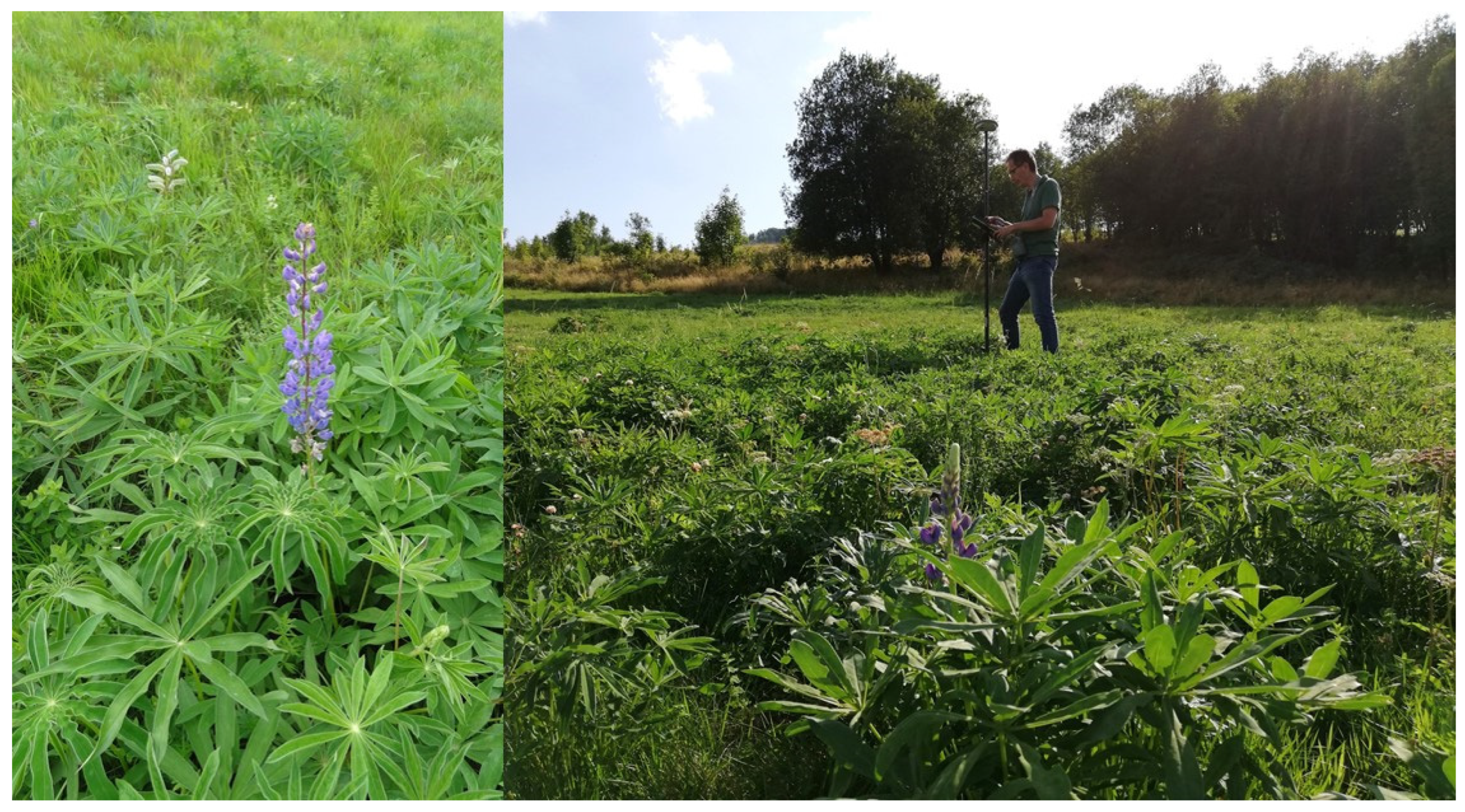
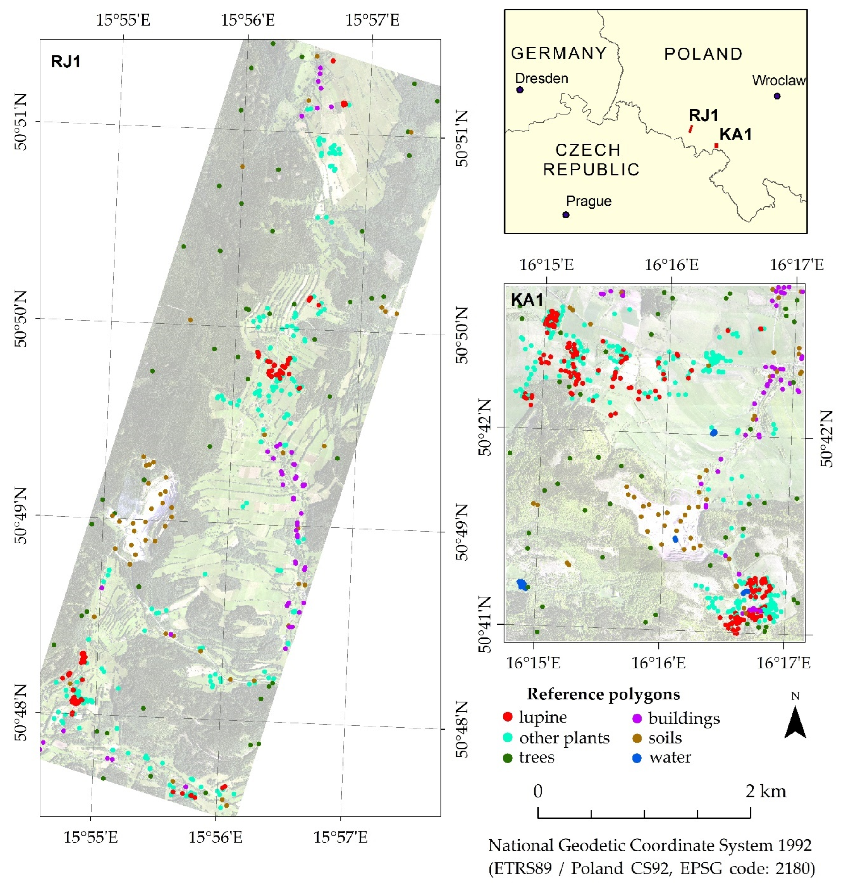
2.1. Research Areas and Objects

Lupinus polyphyllus is a perennial plant of the family Fabaceae, which is native to North America and was intentionally introduced to Europe as an ornamental plant in the 19th century [6]. The species quickly spread, especially in ruderal habitats (roadsides, wastelands, degraded areas) and semi-natural habitats, such as meadows, grasslands, and forest edges. Lupine grows up to 1.5 m in height [59]. It has long, clustered purple or dark blue inflorescences and leaves that form a characteristic rosette (Figure 1). The plant blooms from June to August [60]. Lupine spreads via the vegetative growth of clumps and seeds collected from long, hairy pods. The plant is frost-resistant, insensitive to water shortages, and can easily regenerate after the destruction of the aboveground parts. In addition, this species can fix nitrogen and allelopathically reduce the germination of other plants, leading to significant changes in the structure of plant communities and a decrease in species richness [32,61].
The research was conducted in two research areas located in south-western Poland: the Kamienne Mountains (Natura 2000 site: PLH020038; 9.3 km2; KA1) and Rudawy Janowickie (Natura 2000 site: PLH020011; 13 km2; RJ1); see Figure 2. Both are mountainous areas where the spread of lupines threatens valuable natural habitats protected under the Natura 2000 program, that is, habitat types 6510 (lowland hay meadows) and 6520 (mountain hay meadows). These areas are very heterogeneous because the small meadows belong to different farmers who use different farming practices, such as mowing for hay and cows grazing on pastures.

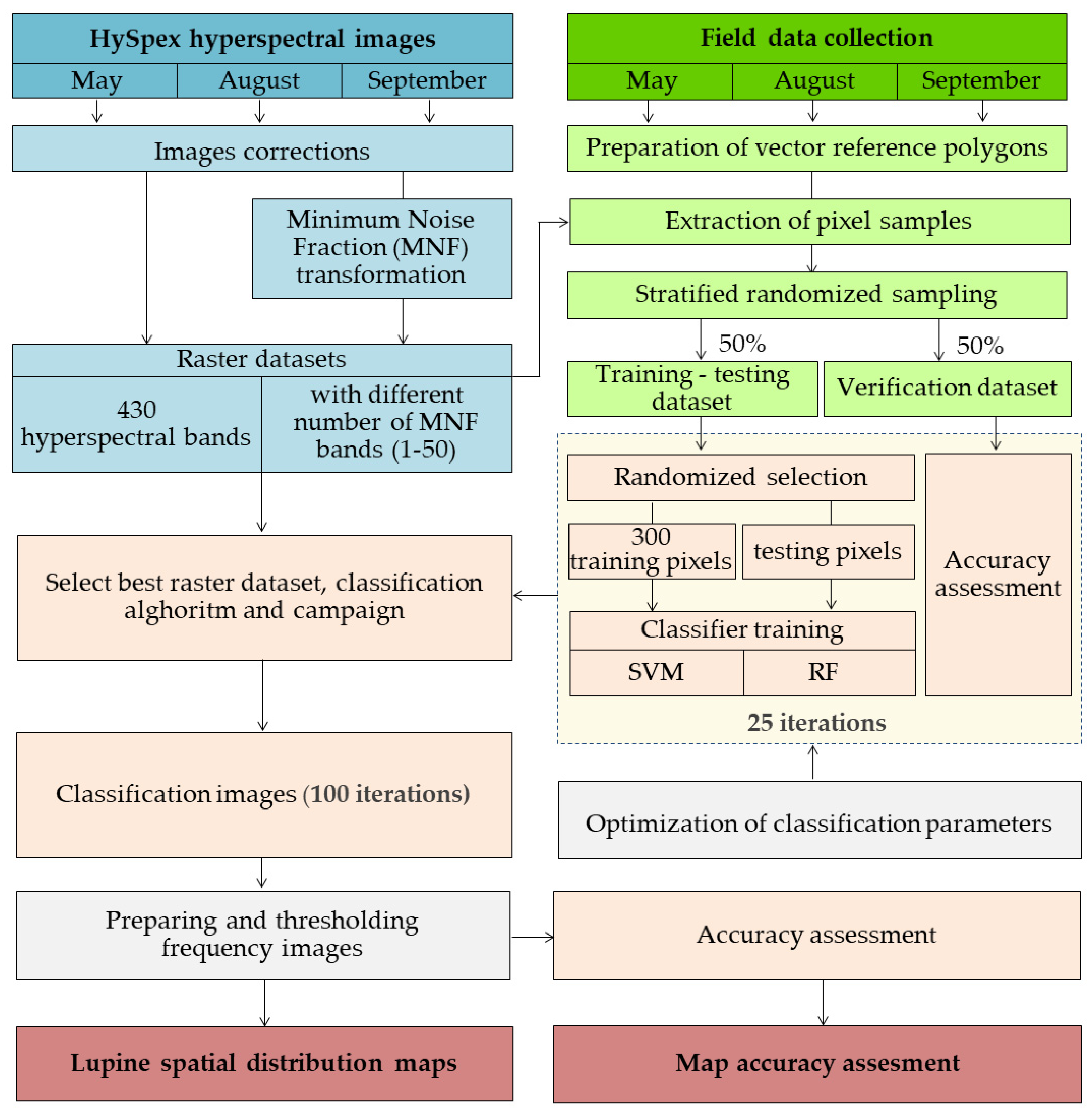
2.2. Research Methodology Overview

The method presented in this article continues and extends previous studies on the identification of invasive plant species using hyperspectral images and machine learning methods [57,58]. This process is divided into the following steps:
  • The acquisition and processing of airborne hyperspectral images.
  • Obtaining and preparing reference field data.
  • Classifier training and iterative accuracy assessment.
  • The preparation of final maps using thresholding frequency images and statistical accuracy reports.
The methodology is presented in the scheme below (Figure 3) and described in detail in the subsequent subsections.

2.3. Airborne HySpex Hyperspectral Images

Aerial hyperspectral images were obtained and processed by the MGGP Aero company three times during the 2016 growing season in both research areas (Table 1). For this purpose, two HySpex VNIR-1800 and SWIR-384 (Norsk Elektro Optikk, Skedsmokorset, Norway) cameras were placed on a Cessna 402 B aircraft [62]. Using the HySpex VNIR-1800 scanner, 182 spectral bands in the range 416–995 nm with a spatial resolution of 0.5 m were acquired; while using the HySpex SWIR-384 sensor, 288 spectral bands in the range 954–2510 nm with a resolution of 1 m were acquired. HySpex RAD software was used to convert the original image digital number (DN) value into a radiation brightness value. Geometric corrections were made using the digital terrain model in PARGE 3.1 software (PARametric GEocoding) [63], and atmospheric corrections were made using the MODTRAN5 algorithm in ATCOR-4 6.2 software (ATmospheric CORrection) [64,65,66]. Hyperspectral data from both sensors were combined and resampled to 1 m spatial resolution, and 19 spectral bands of the HySpex VNIR-1800 scanner were removed due to the overlap in the spectral ranges of both sensors. The last 21 bands in the SWIR range (longer than 2.35 µm) were removed owing to extensive noise, which resulted in 430-band images acquired in the spectral range 416–2396 nm and 16-bit radiometric resolution. An MNF transformation removed noise and compressed the most important information.

2.4. Field Research

Field measurements were conducted a few days after the flight campaigns. Dense patches of lupine and co-occurring plants were located in the research areas, including Aegopodium podagraria L. (goutweed), Arrhenatherum elatius (bulbous oat grass), Cirsium rivulare (plume thistle), Festuca rubra (creeping red fescue), Geranium sylvaticum (wood cranesbill), Petasites hybribus (butterbur), and Urtica dioica (nettle). Based on field measurements (location of plant patches recorded using a GNSS device) and photointerpretation techniques using HySpex images, reference polygons for lupine, surrounding plants, and other land cover types were created (Figure 2).
The polygons covered a square approximately 4 × 4 pixels in size. The number of reference polygons for lupine and co-occurring plants depended on the number of plant patches found during the first field campaign in the study areas. In the area of the Kamienne Mountains, 180 reference polygons were initially established for lupine and 250 for co-occurring plants, while in the Rudawy Janowickie area, there were 100 for lupine and 200 for other plants. For each other land cover class occurring in the studied areas, i.e., trees, soils, buildings, and water, 50 polygons were prepared. The location of the polygons was constant and determined for the first campaign and repeated for subsequent measurement campaigns. If the reference polygon was disturbed in subsequent campaigns (e.g., mowed or shaded), it was removed from the reference set. The final numbers of reference polygons for both areas and individual campaigns are presented in Table 2.
Reference polygons were then randomly divided in a 50/50% ratio into a training–testing set and a validation set. If the number of reference polygons was smaller than that in the first campaign, the number of validation polygons was increased at the expense of the training set to ensure a constant and equal validation set for each campaign (90 polygons for lupines in the KA1 area and 50 polygons for lupines in the RJ1 area). From the set of training–testing polygons, 300 pixels for each class were randomly selected for classifier training. This is the recommended number of training pixels from previous research [57], which is sufficient to identify invasive plant species with high and stable accuracy. Splitting the training–testing and validation sets at the polygon level made the set of validation pixels spatially independent of the training pixels. Moreover, the validation dataset remained unchanged between iterations. Avoiding the spatial autocorrelation of these sets and multiple sampling (separate for each iteration) allowed for a more reliable and objective assessment of accuracy.

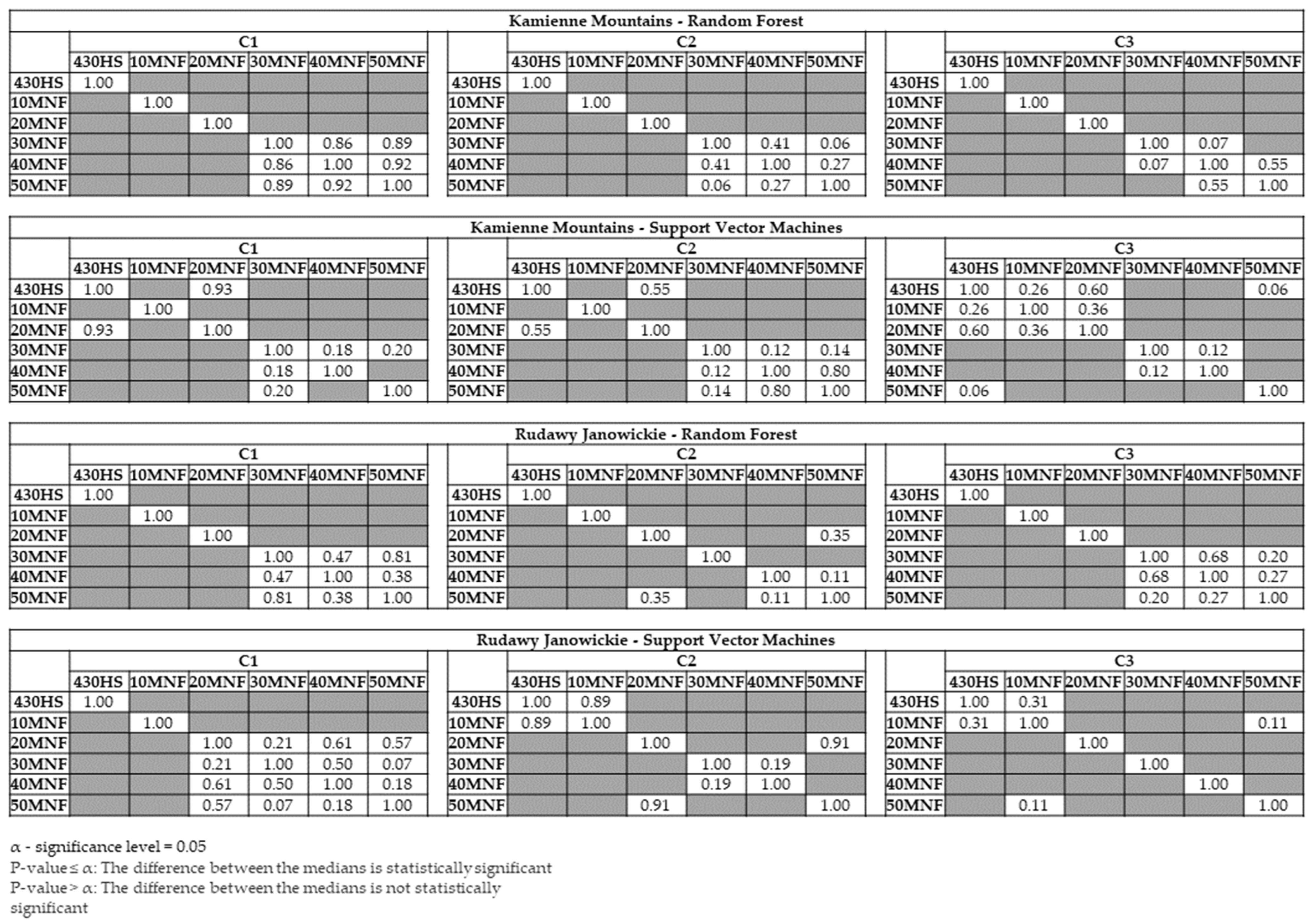
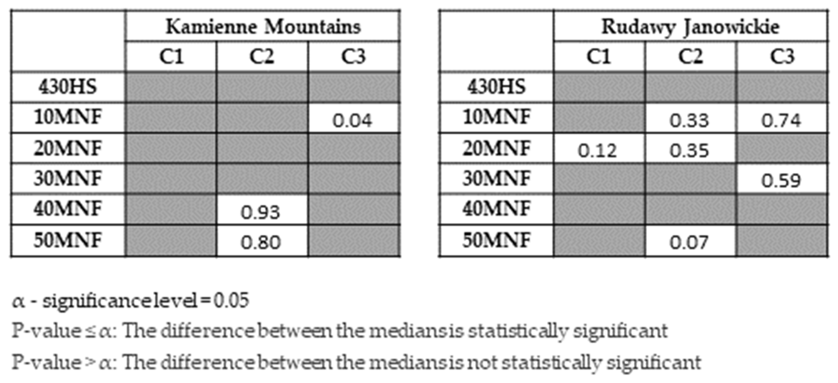
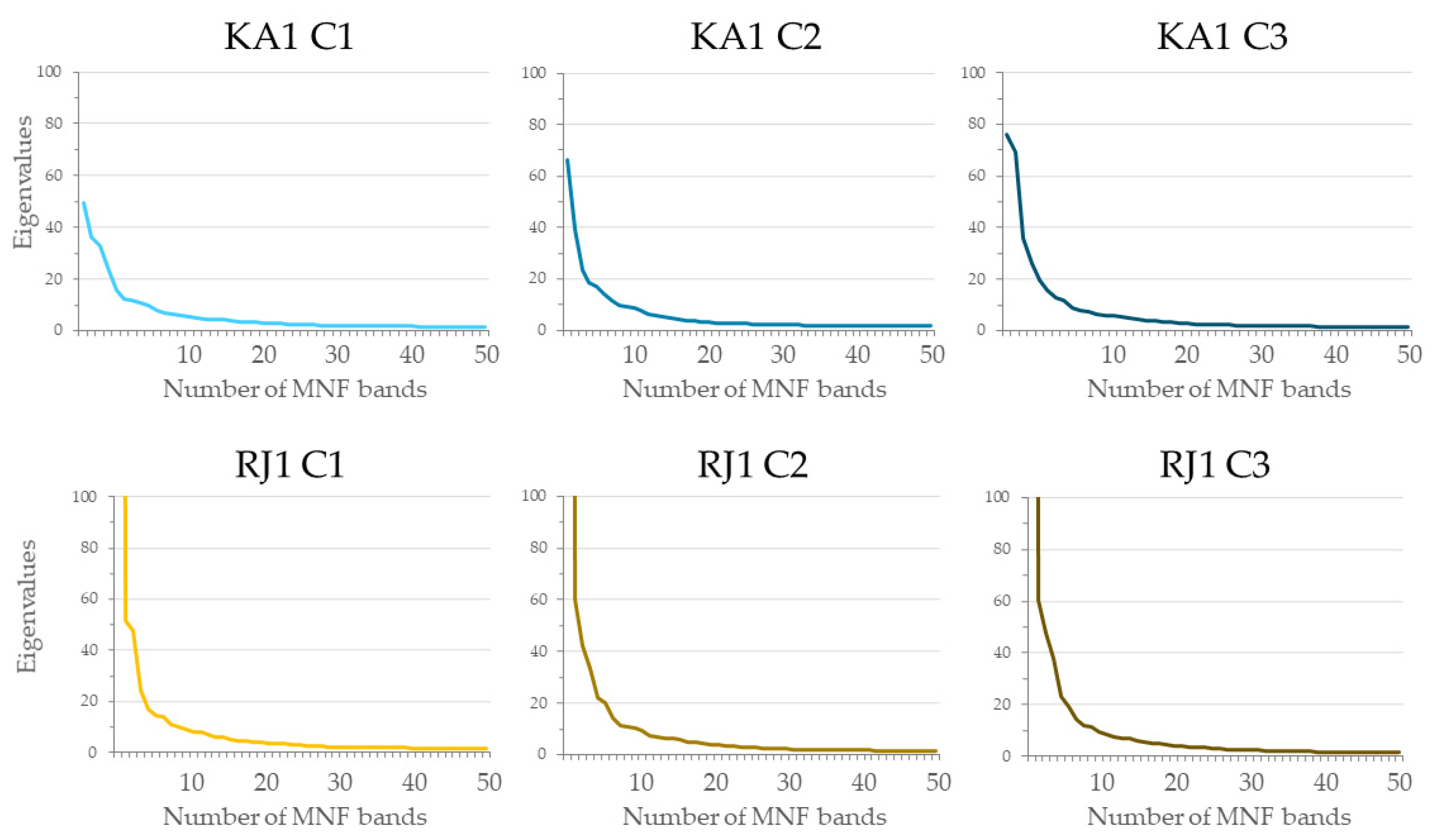
2.5. Classification Process and Accuracy Assessment

The next stage involved testing and optimizing the SVM and RF classification algorithms. The radial basis function (RBF) kernel was chosen for the SVM algorithm due to its effectiveness as confirmed with numerous studies [54,67]. Various penalty costs (10, 100, 1000) and gamma parameters (0.01, 0.1, 0.25, and 0.5) were tested using pixels from the training–testing sets and the grid search method with 10-fold cross validation. Taking error and dispersion into account, the optimal values (gamma: 0.01, cost: 1000 for the spectral bands, and gamma: 0.1 and cost: 1000 for 50 MNF bands) were selected. For the RF, the number of trees was set to 500 and the out-of-bag (OOB) error analysis was performed to select the mtry parameter (number of variables randomly sampled as candidates at each tree branch split). The optimal mtry = 140 was selected for the classification of 430 spectral bands and mtry = 10 was selected for 50 MNF transformation bands.
We used an iterative accuracy assessment method [68,69,70], which enabled a more objective comparison of the results for different input datasets, classification algorithms, or campaigns.
The procedure involved the following steps repeated 25 times:
  • the random selection of 300 training pixels for each class from the training–testing dataset (number of pixels recommended according to a previous study [57]);
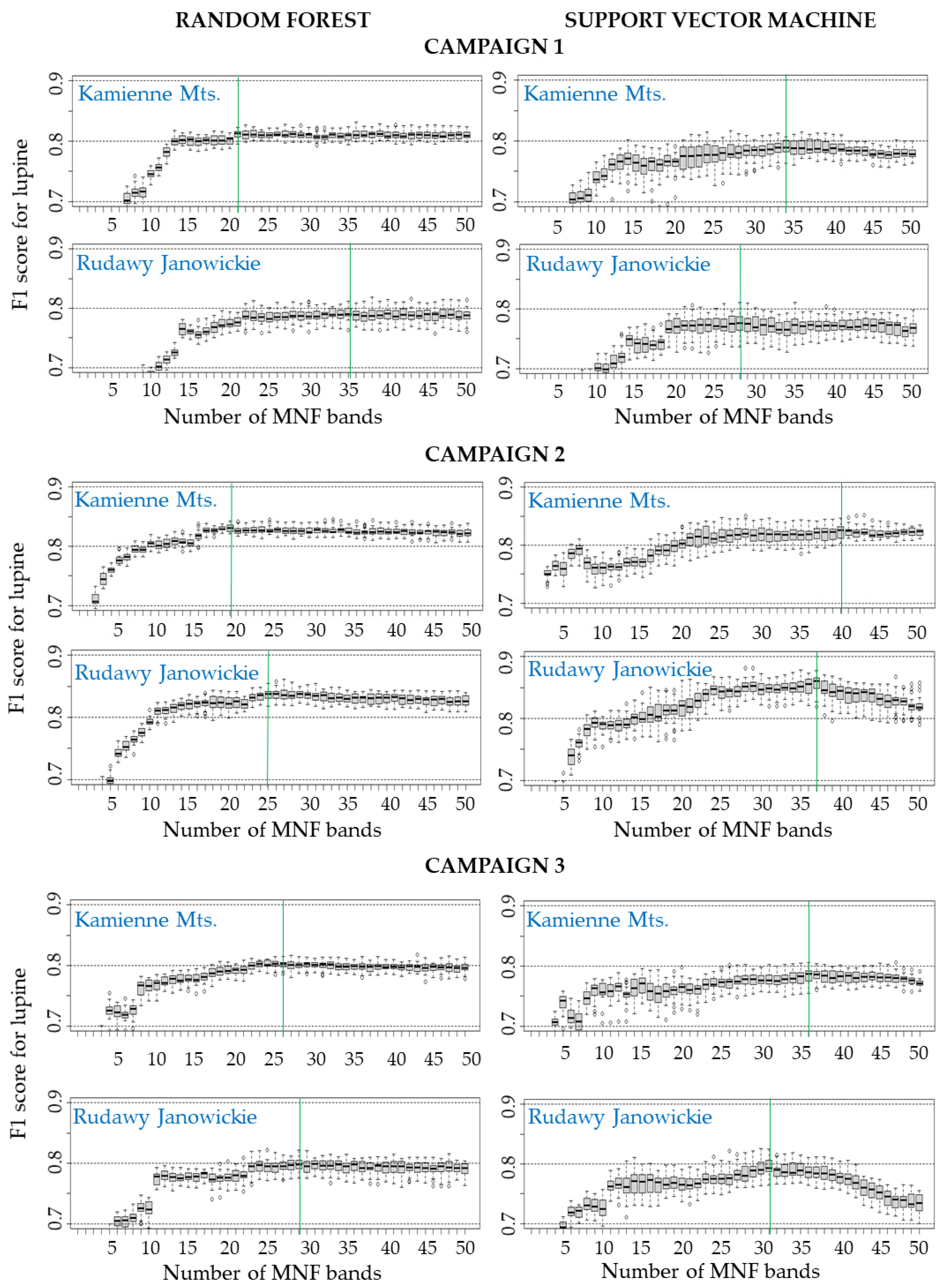
  • RF and SVM classifiers trained on a variable number of MNF bands (from 1 to 50) and a set of 430 HySpex hyperspectral bands for each campaign;
  • accuracy assessment based on the spatially unchanging validation dataset (spatially separated from the training set).
The following parameters were calculated using the confusion matrix: overall accuracy (OA), Cohen’s kappa, producer’s accuracy (PA), user’s accuracy (UA), and F1 score for classes. For each tested data scenario, a boxplot of the F1 score distribution was generated to determine how the selected raster dataset and classifier affected the obtained lupine identification accuracies.
Based on the F1 score distributions for lupine, campaign and raster datasets were selected that allowed for the most accurate identification of lupine in both research areas. The Shapiro–Wilk test was used to check whether the F1 score for lupine was normally distributed. Mann–Whitney–Wilcoxon tests [71] at a significance level of 0.05 were performed to indicate whether there were statistically significant differences between the F1 scores for lupine obtained for various campaigns and raster datasets.

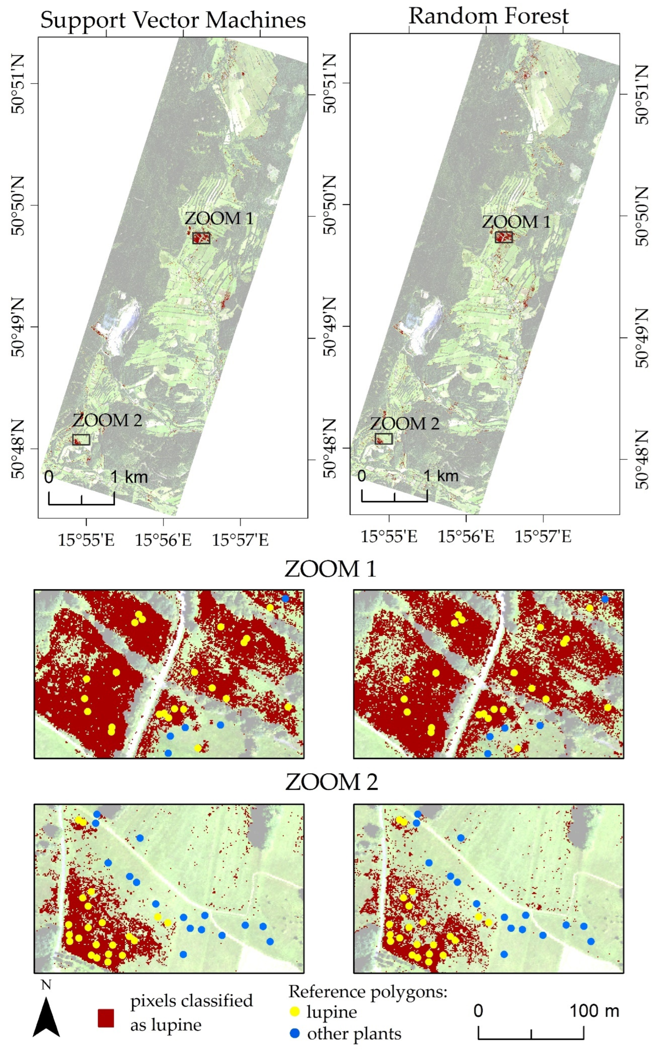
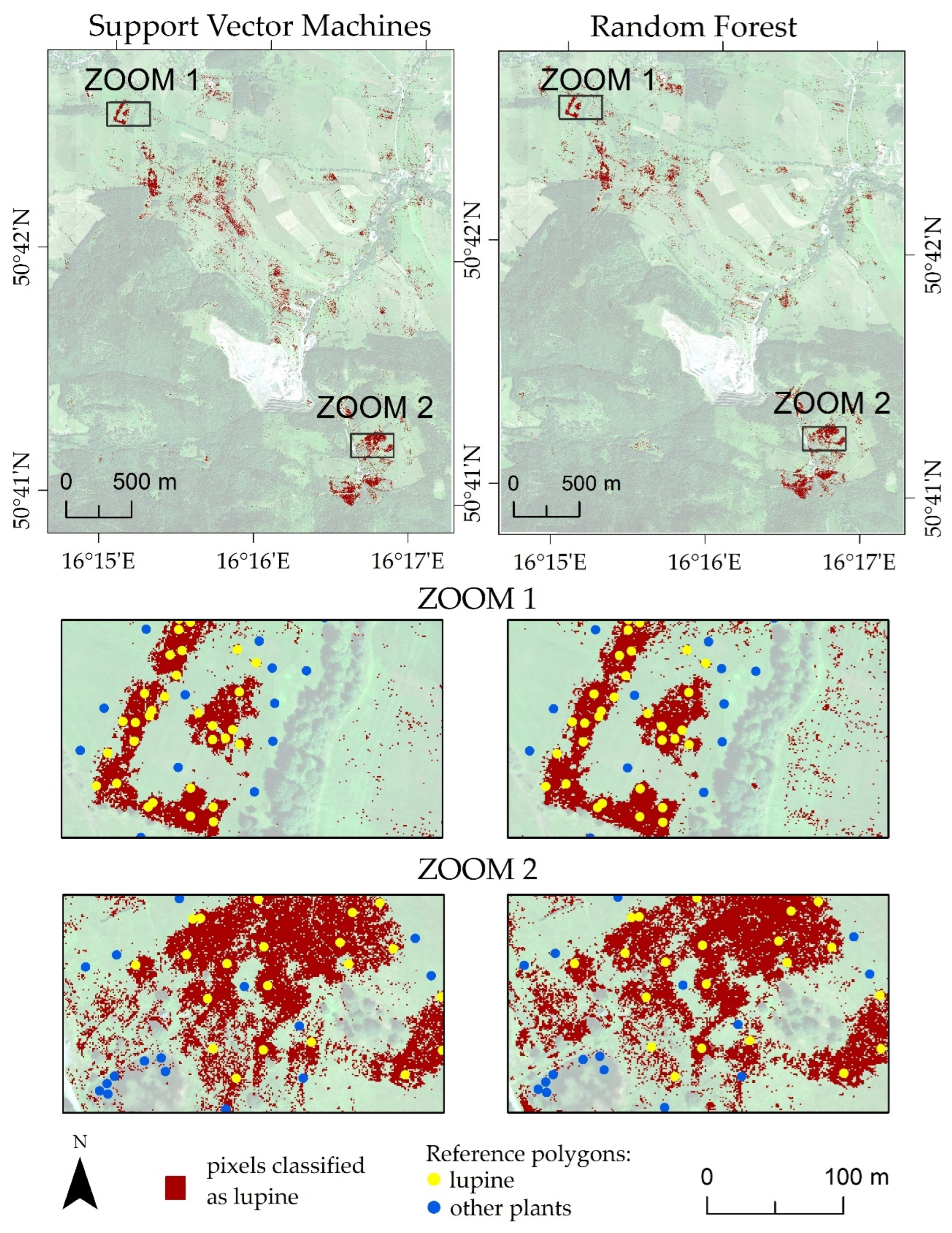
2.6. Image Post-Classification Analysis

For the selected data scenarios (best campaign and raster dataset), the classification and accuracy assessment processes were repeated 100 times. One hundred post-classification images were generated, and the number of lupine occurrences in each pixel of each image was counted to create frequency images. The frequency images were then thresholded to present on the final map only pixels that were consistently indicated by the classifiers as lupine. Following the recommendations from previous research [58], a threshold of 95 was chosen, which indicated pixels recognized by the algorithm as given species for a minimum of 95 out of 100 iterations. This high threshold reduced class overestimation, reduced the salt and pepper effect, and indicated locations that were almost unambiguously identified as lupine.
Accuracy reports, including confusion matrices and classification accuracy parameters (i.e., OA, Cohen’s kappa, PA, and UA), were prepared on the validation datasets that were spatially independent of the training datasets. The verification data for KA1 consisted of 90 reference polygons for lupine and 225 polygons for the background (other plant and land cover classes), whereas the verification set consisted of 50 polygons for lupine and 175 polygons for the background for the RJ1 area.

3. Results

The classifications enabled identifying lupine, with a median F1 score of 0.85 in the area RJ1 and 0.83 in the area KA1. The accuracy increased with the number of MNF bands used in the classification of datasets comprising fewer than 20 bands (Figure 4). The highest accuracies were obtained for classifications performed on about 20 to 40 MNF bands (median F1 score from 0.76 to 0.85 depending on the campaign and classification algorithm). In all analyzed cases (except RF classification in the second campaign and SVM in the third campaign), there were no statistically significant differences between classifications made for 30 and 40 MNF bands (Figure A1 in Appendix A). The use of more than 40 MNF bands did not significantly affect the RF classification accuracy. For the SVM algorithm, this did not significantly improve accuracy or resulted in a reduction in accuracy of up to 6 percentage points. Hence, it can be concluded that the set of 30 MNF bands is the optimal choice for lupine identification, and allows for obtaining the highest accuracies while reducing the data volume and classification time. For the RF algorithm, the interquartile distance for 25 classification iterations on different numbers of MNF bands was smaller than that for the SVM algorithm. Therefore, the results obtained were less variable between the iterations.
The analysis of the eigenvalue graphs generated during the MNF transformations also showed that approximately the first 30 bands of the MNF transformation were the most informative (Figure 5). For the data with respect to each tested campaign, the curves flatten out for more than 30 MNF bands.
The use of 20–40 MNF transformation bands allowed us to obtain up to 0.17 higher F1 scores for lupine compared to that using 430 HySpex spectral bands (Table 3). The accuracies obtained on 430 spectral bands using the SVM algorithm were higher (median F1 score from 0.72 to 0.81) than with the RF algorithm (median F1 score from 0.62 to 0.75, Table 3, Figure A2 in Appendix A).
In both study areas, the highest lupine identification accuracy was obtained during the second campaign (F1 score: 0.85 for RJ1, F1 score: 0.83 for KA1). Considering the scenarios listed in the table above, a median F1 score above 0.8 was most often obtained for this campaign (C2). At the beginning of August (C2), lupine was at its peak of growth; it bloomed and filled large, compact patches, which made it easier to identify. Statistically significant lower accuracies were obtained in the spring (F1 score: 0.81) and autumn (F1 score: 0.80) campaigns (Table 3, Figure A3 in Appendix A). During the first campaign in May (C1), lupine was identified before the flowering period and some specimens were still small and visually similar to co-occurring plants. In the third campaign (September C3), lupine inflorescences were withered, and some of the plant patches were attacked by a fungal disease of lupine, i.e., powdery mildew (Erysiphe pisi). The use of meadows and pastures, especially mowing and grazing of animals, also made identification difficult. For campaign C1, the highest median F1 score (SVM: 0.79, RF: 0.81) for lupine was obtained for scenarios using 30–50 MNF bands (Figure 4, Table 3) for both research areas. For campaign C2, the highest F1 scores (SVM: 0.85, RF: 0.84) were obtained for 20–40 MNF bands in KA1 and 30 MNF bands in RJ1. Campaign C3 showed similar tendencies, with scenarios using 30 and 40 MNF bands achieving the highest F1 scores (SVM: 0.79, RF: 0.80). The results show that, regardless of the time of data acquisition (campaign) or study area, the datasets containing 30 and 40 MNF bands performed best. Space used on a hard disk (HDD) for 30 MNF bands was more than 5 times lower than the full set of original hyperspectral bands. Moreover, in the best-case scenarios, both the RF and SVM algorithms obtained comparable results (a maximum difference of two percentage points).
Based on the above results, 30 MNF bands from the second campaign (C2) were used to prepare the final lupine maps for both research areas. Pixels classified by RF and SVM classifiers as lupine a minimum of 95 times (out of 100 iterations) are marked in red on the maps below (Figure 6 and Figure 7).
Maps obtained using thresholding frequency images in the KA1 area achieved similar map accuracies for both classification methods (OA: 89%, Cohen’s kappa: 0.73, F1 score for lupine: 0.80, Table 4). Lupine invasions were mainly located in the meadows and pastures in the northwest and southeast regions of the area.
Both post-classification images had an omission error of approximately 29%, especially in places where the lupine density was lower (over 20% of the reference polygon for lupines covered with co-occurring species). Some patches of lupine were poorly regrown after mowing or grazing by farm animals. A possible reason for the underestimation was also the use of a high threshold, which resulted in the rejection of less reliable pixels classified as lupins from the final map.
The overestimation error on both maps was approximately 9% and occurred where visually similar plants, such as butterbur (Petasites hybribus), nettle, meadow thistle (Cirsium rivulare), and bulbous oat grass, grew.
In the Rudawy Janowickie area, the SVM method yielded a higher identification accuracy (OA: 94%, Cohen’s kappa: 0.82, F1 score for lupine: 0.86) than the RF algorithm (OA: 93%, Cohen’s kappa: 0.78, F1 score for lupine: 0.83, Table 5). The overestimation error for the lupine class was lower in the support vector machine image (8%) than in the RF image (12%), and the lupines were mostly mixed with tall grasses, that is, bulbous oat grass.

4. Discussion

In this paper, we have presented the original processing chain for invasive species mapping using machine learning algorithms and hyperspectral data. The presented method of multiple classification and thresholding of frequency images allows the results of many inferred images to be included in the final map. The final maps show only those pixels that were classified as lupine in 95 out of 100 classification iterations, based on a random selection of training and validation patterns from field polygons. This increases the reliability of the results and reduces the “salt and pepper” effect. Despite the similarity of Lupinus polyphyllus to co-occurring plants (similar leaf color and physiological characteristics to native plants, occurring in heterogeneous, small patches), it was possible to identify this species using the SVM and RF algorithms with satisfactory accuracy (F1 score from 0.8 to 0.86) in two research areas. The high potential and repeatability of the method were also confirmed in a different location in Poland (Malinowice village), where wood small-reed, blackberry, and goldenrod were identified with high accuracies (F1 score above 0.9, [57,58]). However, these species were more distinguishable from the surrounding plants than lupines because of their characteristic inflorescences and their occurrence in large and dense patches.
It can be concluded that the Lupinus polyphyllus identification results using both machine learning algorithms (RF and SVM) were similar (F1 score for lupine: 0.8 and OA: 89% in the Kamienne Mountains area and F1 scoreRF: 0.83, OARF: 93%, F1 score SVM: 0.86, and OASVM: 94% in the Rudawy Janowickie area). The methods used by other researchers to identify lupines have yielded similar accuracies to those presented in this article (Table 6); however, they refer to a different spatial scale [32,72,73]. The identification of lupine in the UNESCO biosphere reserve “Rhön” in Germany using UAV RGB, thermal imagery, and an object-based image analysis (OBIA) with the RF algorithm gave a similar mean overall accuracy of approximately 89%, but some models highly overestimated the results (false positive rate up to 47%) [72]. A further comparison of the results is difficult because of the lack of reported class-accuracy metrics for individual classes in the above-mentioned studies. The object classification method worked well for data with very high spatial resolution (0.5 m), but the research was limited to a small area (1.5 km2) due to the capabilities of the drone (DJI-Phantom IV quadcopter). Lupine identification has also been carried out in the same reserve using WorldView-3 satellite data and the gradient-boosting machine method [32], but a lower classification accuracy was obtained (F1 score for lupine: 0.76) than those presented in the present article. Panchromatic and multispectral data from this satellite enabled a prediction map to be obtained for a larger “Leitgraben” area, but the authors noted that only large patches of lupine (area at least 3 × 3 m2) were detected. Similar conclusions were drawn when identifying another lupine species, Lupinus nootkatensis, in Iceland using SPOT 5 images [73]. The authors used a maximum likelihood classifier to achieve high accuracy (OA: 94% and Kappa: 0.88); however, they observed that sparse and freestanding lupine areas and patches with a combination of other vegetation were not detected. However, these small, solitary patches of lupine are indicated as the main factor causing the spread of this species into new areas. Low accuracies for white and yellow lupine (F1 score below 0.04) were also obtained when mapping annual crops in Portugal using Sentinel-2 data and the random forest method [74]. This confirms that, in the case of lupine identification, high spatial and spectral resolutions of the images are important, especially if the beginning of the invasion is to be detected.
In this paper, the impact of the number of MNF bands used on the accuracy achieved was also analyzed. The accuracy of lupine classification increased with the number of MNF bands in the input set but stabilized for sets consisting of more than 20 transformed bands. Datasets containing about the first 30 MNF bands gave the highest classification accuracies (median F1 score for lupine from 0.77 to 0.85), while accuracies obtained for the 430 HySpex spectral bands were lower (median F1 score from 0.62 to 0.81). Improvements in species identification accuracy after using dimensionality reduction methods have also been noted in other studies [28,30]. The use of 30 MNF bands to classify small-reed wood, goldenrod, and blackberry in southern Poland resulted in higher average F1 score accuracies for the three species (F1: 0.86–0.91) compared to the results with 430 HySpex hyperspectral bands (F1: 0.93–0.95, [57]). The use of 20 MNF bands resulted in higher classification accuracies for seven tree species for RF (OA: 87%) and a multi-class classifier (MCC, OA: 89%), compared to using 118 HyMap bands (OA: 46% for RF and OA: 79% for MCC) [29]. Additionally, testing different raster data (MNF bands from HySpex data, lidar products, and vegetation indices) for the identification of steeplebush (Spiraea tomentosa) in the Lower Silesian forests gave the highest RF classification accuracies for 25 MNF bands (OA: 99%, F1 score for steeplebush: 0.83) and the obtained accuracies were similar to those for lupine in this article [19].
The study showed that the best period for mapping lupines was the second campaign (August). The F1 score for lupine obtained in the summer campaign (SVM up to 0.85; RF up to 0.84) was higher than that in the other campaigns. Other authors have also shown that the beginning of September is not the best time to identify lupines in central Europe (Germany) and recommended collecting data during the peak flowering period of Lupinus polyphyllus [32]. The campaign during the flowering period of the identified plants (August) was also optimal for classifying small-reed wood (F1: 0.90) and blackberry (0.98), whereas goldenrod was well identified in every campaign (F1 from 0.96 to 0.99) [58]. Similar conclusions were reached during the classification of Echinocystis lobata in the Bzura River valley in central Poland using the RF algorithm and HySpex images [9]. The F1 score for the species was the highest in summer (0.87) and was lower in spring (F1: 0.64) and autumn (F1: 0.75). The blooming time was also the best period for identifying Molinia caerulea; in August, the F1 score for this species ranged from 0.86 to 0.89, while the accuracy was lower in June (F1 score from 0.78 to 0.87) and September (F1 score from 0.84 to 0.88) [20]. Significant differences in the accuracy obtained depending on the time of data acquisition were also observed during Carduus nutans identification using the SVM algorithm and AISA data, when OA = 91% was obtained for the peak flowering period for musk thistle (June) and OA = 79% was obtained before flowering (April) [76]. The variability in the spectral characteristics of co-occurring plants is also worthy of attention. In the case of steeplebush identification, a higher F1 for the species was obtained for the September campaign (F1: 82.96%) compared to the August campaign (F1: 77.25%) [19]. The woody parts of the steeplebush were more visible in autumn, owing to changes in the spectral characteristics of the surrounding plants and lower biomass.

5. Conclusions

Monitoring the spread of invasive plant species in protected areas is crucial for implementing appropriate management and control programs that will limit the negative effects of the invasion. In this paper, using the example of lupine, we presented step-by-step how to reliably map invasive species using HySpex hyperspectral data and machine learning methods. The proposed methodology of the multiple classification and thresholding of frequency images allows the results of multiple predictions to be included in the final map, which improves the quality and reliability of species maps created for control purposes.
The following conclusions were drawn:
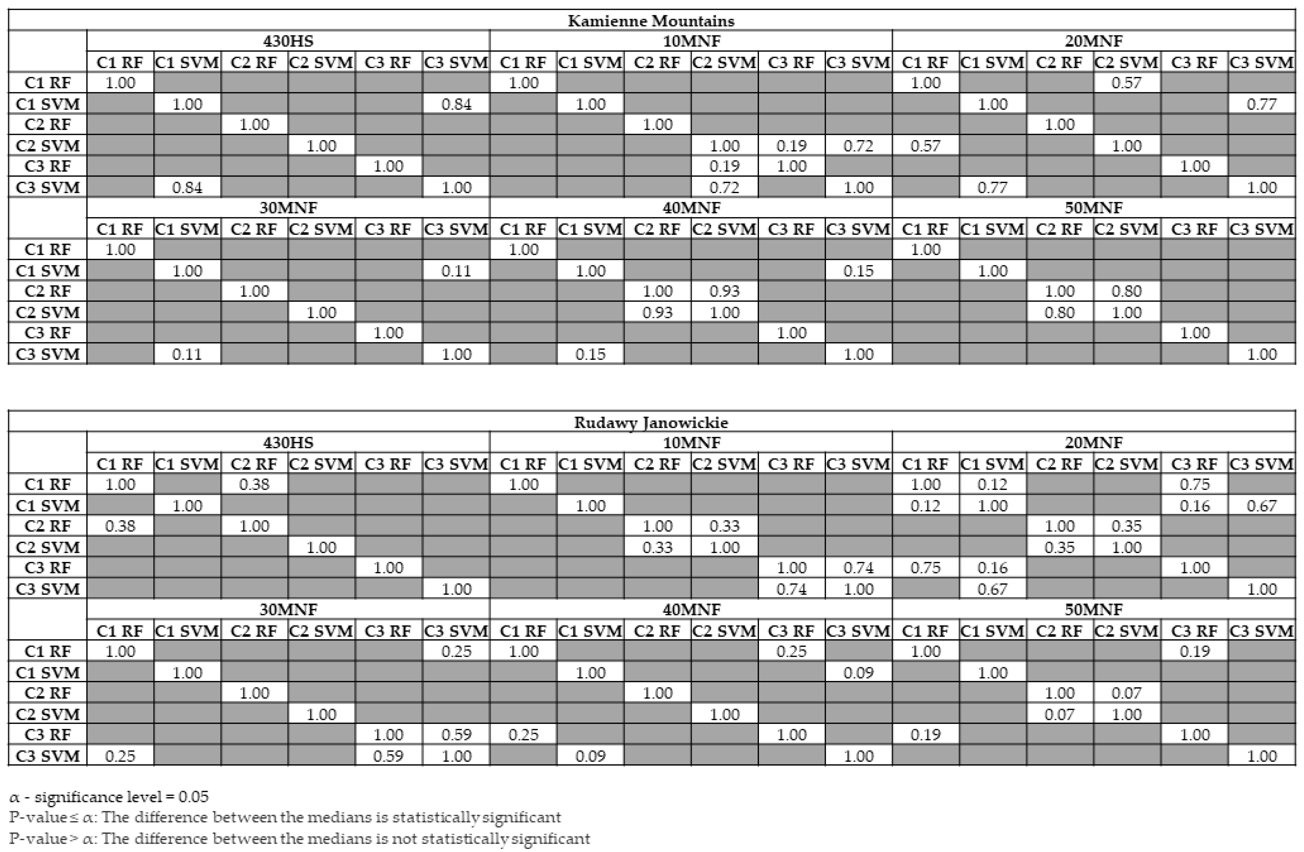
  • The results show that aerial and field data should be collected at the peak of flowering of the identified plant to obtain the most accurate maps. The highest accuracy of the lupine class in both research areas was obtained during the summer campaign (August, median F1 score ranging from 0.82 to 0.85). Statistically significantly lower accuracies were obtained for the spring (F1 score: 0.77–0.81) and autumn (F1 score: 0.78–0.80) campaigns.
  • The use of approximately 30 MNF bands must be considered for classification purposes when hyperspectral data are used. Input datasets consisting of 30 MNF bands produced the highest accuracies for the lupine class (median F1 score ranging from 0.77 to 0.85), and the use of a higher number of MNF bands did not significantly increase the identification accuracy. The classification accuracies obtained on the original 430 spectral bands were lower (median F1 score from 0.62 to 0.81) in both study areas.
  • The classifiers gave similar results for lupine identification in both research areas (F1 score: 0.80–0.86), which confirms that both RF and SVMs can be successfully used to identify IAS.
In the next stages of research, consideration should be given to checking whether the presented method can be applied to publicly available satellite data and what information loss this may cause. Multispectral data from satellites, e.g., Sentinel-2 or WorldView-4, could reduce costs and provide the ability to frequently acquire data for large areas to update existing maps. However, they may be insufficient to detect the beginnings of an invasion, especially in the case of plant species that are spectrally similar to the surroundings. It would also be possible to consider using other algorithms, e.g., deep neural networks or object-based classification, on high-spatial-resolution UAV data [77,78,79].

Author Contributions

Conceptualization, methodology: A.S.-T., E.R., and B.Z.; software: A.S.-T. and E.R.; validation: A.S.-T. and B.Z.; formal analysis, investigation: A.S.-T. and E.R.; resources, data curation, writing—original draft preparation: A.S.-T.; writing—review and editing: all authors; visualization: A.S.-T.; supervision: B.Z. and E.R.; funding acquisition: A.S.-T. and B.Z. All authors have read and agreed to the published version of the manuscript.

Funding

This research was funded by the Polish National Centre for Research and Development (NCBiR) under the program “Natural Environment, Agriculture and Forestry BIOSTRATEG II.: The innovative approach supporting monitoring of non-forest Natura 2000 habitats, using remote sensing methods (HabitARS)”, grant number: DZP/BIOSTRATEG-II/390/2015; the Consortium Leader is MGGP Aero. The project partners include the University of Lodz, the University of Warsaw, Warsaw University of Life Sciences, the Institute of Technology and Life Sciences, the University of Silesia in Katowice, and Warsaw University of Technology. The costs of language correction were covered by the Faculty of Geography and Regional Studies of the University of Warsaw, grant number: SWIB 2/2024.

Data Availability Statement

The airborne HySpex hyperspectral images used in this study were acquired and preprocessed by the MGGP Aero company, which is the leader of the HabitARS consortium. Field data were acquired by Anita Sabat-Tomala and Bogdan Zagajewski. The data are not publicly available.

Acknowledgments

The authors would like to thank the whole HabitARS Consortium for their work on the HabitARS project, especially the MGGP Aero company, which acquired and processed the HySpex images. Field data were acquired in the frame of the statutory activity of young researchers (PhD students) of the Faculty of Geography and Regional Studies, University of Warsaw. In the period 2019–2020, Fundacja im. Anny Pasek (Anna Pasek Foundation) supported the research activity of Anita Sabat-Tomala, who is the Foundation scholarship holder.

Conflicts of Interest

The authors declare no conflicts of interest.

Appendix A

Figure A1. Results of the Mann–Whitney–Wilcoxon tests of statistical significance of differences between obtained accuracies for various raster datasets (430HS—430 HySpex spectral bands, 10/20/30/40/50MNF—number of minimum noise fraction transformation bands), grouped by the campaigns (C1—May, C2—August, C3—September) and classifiers (random forest and support vector machine) in two research areas—Kamienne Mountains and Rudawy Janowickie. The significance level was 0.05. Statistically significant differences between various raster datasets are grayed out. The significance level was 0.05.
Remotesensing 16 00580 g0a1
Figure A2. Results of the Mann–Whitney–Wilcoxon tests of statistical significance of differences between support vector machine (SVM) and random forest (RF) results, grouped by the campaigns (C1—May, C2—August, C3—September) and raster data used (430HS—430 HySpex spectral bands, 10/20/30/40/50MNF—number of minimum noise fraction transformation bands) for two research areas—Kamienne Mountains and Rudawy Janowickie. Statistically significant differences between random forest and support vector machine algorithms are grayed out.
Remotesensing 16 00580 g0a2
Figure A3. Results of the Mann–Whitney–Wilcoxon tests of statistical significance of differences between obtained accuracies for different campaigns (C1—May, C2—August, C3—September) and both classifiers (RF—random forest and SVM—support vector machine), grouped by the raster data used (430HS—430 HySpex spectral bands, 10/20/30/40/50MNF—number of minimum noise fraction transformation bands) for two research areas—Kamienne Mountains and Rudawy Janowickie. Statistically significant differences between campaigns and algorithms are grayed out.
Remotesensing 16 00580 g0a3

References

  1. Seebens, H.; Essl, F.; Dawson, W.; Fuentes, N.; Moser, D.; Pergl, J.; Pyšek, P.; van Kleunen, M.; Weber, E.; Winter, M.; et al. Global Trade Will Accelerate Plant Invasions in Emerging Economies under Climate Change. Glob. Chang. Biol. 2015, 21, 4128–4140. [Google Scholar] [CrossRef]
  2. Sittaro, F.; Hutengs, C.; Vohland, M. Which Factors Determine the Invasion of Plant Species? Machine Learning Based Habitat Modelling Integrating Environmental Factors and Climate Scenarios. Int. J. Appl. Earth Obs. Geoinf. 2023, 116, 103158. [Google Scholar] [CrossRef]
  3. Kumar Rai, P.; Singh, J.S. Invasive Alien Plant Species: Their Impact on Environment, Ecosystem Services and Human Health. Ecol. Indic. 2020, 111, 106020. [Google Scholar] [CrossRef] [PubMed]
  4. Gallardo, B.; Clavero, M.; Sánchez, M.I.; Vilà, M. Global Ecological Impacts of Invasive Species in Aquatic Ecosystems. Glob. Chang. Biol. 2016, 22, 151–163. [Google Scholar] [CrossRef] [PubMed]
  5. Haubrock, P.J.; Turbelin, A.J.; Cuthbert, R.N.; Novoa, A.; Taylor, N.G.; Angulo, E.; Ballesteros-Mejia, L.; Bodey, T.W.; Capinha, C.; Diagne, C.; et al. Economic Costs of Invasive Alien Species across Europe. NeoBiota 2021, 67, 153–190. [Google Scholar] [CrossRef]
  6. Ludewig, K.; Klinger, Y.P.; Donath, T.W.; Bärmann, L.; Eichberg, C.; Thomsen, J.G.; Görzen, E.; Hansen, W.; Hasselquist, E.M.; Helminger, T.; et al. Phenology and Morphology of the Invasive Legume Lupinus polyphyllus along a Latitudinal Gradient in Europe. NeoBiota 2022, 78, 185–206. [Google Scholar] [CrossRef]
  7. Lambdon, P.W.; Pyšek, P.; Basnou, C.; Hejda, M.; Arianoutsou, M.; Essl, F.; Jarošík, V.; Pergl, J.; Winter, M.; Anastasiu, P.; et al. Alien Flora of Europe: Species Diversity, Temporal Trends, Geographical Patterns and Research Needs. Preslia 2008, 80, 101–149. [Google Scholar]
  8. Walsh, S.J. Multi-Scale Remote Sensing of Introduced and Invasive Species: An Overview of Approaches and Perspectives; Springer: Cham, Switzerland, 2018; pp. 143–154. [Google Scholar]
  9. Kopeć, D.; Zakrzewska, A.; Halladin-Dąbrowska, A.; Wylazłowska, J.; Sławik, Ł. The Essence of Acquisition Time of Airborne Hyperspectral and On-Ground Reference Data for Classification of Highly Invasive Annual Vine Echinocystis lobata (Michx.) Torr. & A. Gray. GIScience Remote Sens. 2023, 60, 2204682. [Google Scholar] [CrossRef]
  10. Bradley, B.A. Remote Detection of Invasive Plants: A Review of Spectral, Textural and Phenological Approaches. Biol. Invasions 2014, 16, 1411–1425. [Google Scholar] [CrossRef]
  11. Duncan, P.; Podest, E.; Esler, K.J.; Geerts, S.; Lyons, C. Mapping Invasive Herbaceous Plant Species with Sentinel-2 Satellite Imagery: Echium Plantagineum in a Mediterranean Shrubland as a Case Study. Geomatics 2023, 3, 328–344. [Google Scholar] [CrossRef]
  12. Theron, K.J.; Pryke, J.S.; Latte, N.; Samways, M.J. Mapping an Alien Invasive Shrub within Conservation Corridors Using Super-Resolution Satellite Imagery. J. Environ. Manag. 2022, 321, 116023. [Google Scholar] [CrossRef] [PubMed]
  13. Qian, W.; Huang, Y.; Liu, Q.; Fan, W.; Sun, Z.; Dong, H.; Wan, F.; Qiao, X. UAV and a Deep Convolutional Neural Network for Monitoring Invasive Alien Plants in the Wild. Comput. Electron. Agric. 2020, 174, 105519. [Google Scholar] [CrossRef]
  14. Bakacsy, L.; Tobak, Z.; van Leeuwen, B.; Szilassi, P.; Biró, C.; Szatmári, J. Drone-Based Identification and Monitoring of Two Invasive Alien Plant Species in Open Sand Grasslands by Six RGB Vegetation Indices. Drones 2023, 7, 207. [Google Scholar] [CrossRef]
  15. Cierniewski, J.; Ceglarek, J.; Karnieli, A.; Królewicz, S.; Kaźmierowski, C.; Zagajewski, B. Predicting the diurnal blue-sky albedo of soils using their laboratory reflectance spectra and roughness indices. J. Quant. Spectrosc. Radiat. Transf. 2017, 200, 25–31. [Google Scholar] [CrossRef]
  16. Zagajewski, B.; Kycko, M.; Tømmervik, H.; Bochenek, Z.; Wojtuń, B.; Bjerke, J.W.; Kłos, A. Feasibility of Hyperspectral Vegetation Indices for the Detection of Chlorophyll Concentration in Three High Arctic Plants: Salix Polaris, Bistorta Vivipara, and Dryas Octopetala. Acta Soc. Bot. Pol. 2018, 87, 3604. [Google Scholar] [CrossRef]
  17. Kycko, M.; Zagajewski, B.; Zwijacz-Kozica, M.; Cierniewski, J.; Romanowska, E.; Orłowska, K.; Ochtyra, A.; Jarocińska, A. Assessment of Hyperspectral Remote Sensing for Analyzing the Impact of Human Trampling on Alpine Swards. Mt. Res. Dev. 2017, 37, 66–74. [Google Scholar] [CrossRef]
  18. Cavender-Bares, J.; Gamon, J.A.; Townsend, P.A. (Eds.) Remote Sensing of Plant Biodiversity; Springer International Publishing: Cham, Switzerland, 2020; ISBN 978-3-030-33156-6. [Google Scholar]
  19. Kopeć, D.; Sabat-Tomala, A.; Michalska-Hejduk, D.; Jarocińska, A.; Niedzielko, J. Application of Airborne Hyperspectral Data for Mapping of Invasive Alien Spiraea tomentosa L.: A Serious Threat to Peat Bog Plant Communities. Wetl. Ecol. Manag. 2020, 28, 357–373. [Google Scholar] [CrossRef]
  20. Marcinkowska-Ochtyra, A.; Jarocińska, A.; Bzdęga, K.; Tokarska-Guzik, B. Classification of Expansive Grassland Species in Different Growth Stages Based on Hyperspectral and LiDAR Data. Remote Sens. 2018, 10, 2019. [Google Scholar] [CrossRef]
  21. Huang, Y.; Li, J.; Yang, R.; Wang, F.; Li, Y.; Zhang, S.; Wan, F.; Qiao, X.; Qian, W. Hyperspectral Imaging for Identification of an Invasive Plant Mikania Micrantha Kunth. Front. Plant Sci. 2021, 12, 626516. [Google Scholar] [CrossRef]
  22. Papp, L.; van Leeuwen, B.; Szilassi, P.; Tobak, Z.; Szatmári, J.; Árvai, M.; Mészáros, J.; Pásztor, L. Monitoring Invasive Plant Species Using Hyperspectral Remote Sensing Data. Land 2021, 10, 29. [Google Scholar] [CrossRef]
  23. Gite, H.R.; Solankar, M.M.; Surase, R.R.; Kale, K.V. Comparative Study and Analysis of Dimensionality Reduction Techniques for Hyperspectral Data. In Communications in Computer and Information Science; Springer: Singapore, 2019; Volume 1035, pp. 534–546. ISBN 9789811391804. [Google Scholar]
  24. Royimani, L.; Mutanga, O.; Odindi, J.; Dube, T.; Matongera, T.N. Advancements in Satellite Remote Sensing for Mapping and Monitoring of Alien Invasive Plant Species (AIPs). Phys. Chem. Earth Parts A/B/C 2019, 112, 237–245. [Google Scholar] [CrossRef]
  25. Hotelling, H. Analysis of a Complex of Statistical Variables into Principal Components. J. Educ. Psychol. 1933, 24, 417–441. [Google Scholar] [CrossRef]
  26. Comon, P. Independent Component Analysis, A New Concept? Signal Process. 1994, 36, 287–314. [Google Scholar] [CrossRef]
  27. Green, A.A.; Berman, M.; Switzer, P.; Craig, M.D. A Transformation for Ordering Multispectral Data in Terms of Image Quality with Implications for Noise Removal. IEEE Trans. Geosci. Remote Sens. 1988, 26, 65–74. [Google Scholar] [CrossRef]
  28. Murinto, M.; Dyah, N.R. Feature Reduction Using the Minimum Noise Fraction and Principal Component Analysis Transforms for Improving the Classification of Hyperspectral Images. Asia-Pac. J. Sci. Technol. 2017, 22, 1–15. [Google Scholar] [CrossRef]
  29. Zhang, Z.; Kazakova, A.; Moskal, L.; Styers, D. Object-Based Tree Species Classification in Urban Ecosystems Using LiDAR and Hyperspectral Data. Forests 2016, 7, 122. [Google Scholar] [CrossRef]
  30. Burai, P.; Deák, B.; Valkó, O.; Tomor, T. Classification of Herbaceous Vegetation Using Airborne Hyperspectral Imagery. Remote Sens. 2015, 7, 2046–2066. [Google Scholar] [CrossRef]
  31. Müllerová, J.; Brůna, J.; Bartaloš, T.; Dvořák, P.; Vítková, M.; Pyšek, P. Timing Is Important: Unmanned Aircraft vs. Satellite Imagery in Plant Invasion Monitoring. Front. Plant Sci. 2017, 8, 887. [Google Scholar] [CrossRef]
  32. Schulze-Brüninghoff, D.; Wachendorf, M.; Astor, T. Potentials and Limitations of WorldView-3 Data for the Detection of Invasive Lupinus polyphyllus Lindl. in Semi-Natural Grasslands. Remote Sens. 2021, 13, 4333. [Google Scholar] [CrossRef]
  33. Mundt, J.; Glenn, N.; Weber, K.; Prather, T.; Lass, L.; Pettingill, J. Discrimination of Hoary Cress and Determination of Its Detection Limits via Hyperspectral Image Processing and Accuracy Assessment Techniques. Remote Sens. Environ. 2005, 96, 509–517. [Google Scholar] [CrossRef]
  34. Bustamante, J.; Aragonés, D.; Afán, I.; Luque, C.; Pérez-Vázquez, A.; Castellanos, E.; Díaz-Delgado, R. Hyperspectral Sensors as a Management Tool to Prevent the Invasion of the Exotic Cordgrass Spartina Densiflora in the Doñana Wetlands. Remote Sens. 2016, 8, 1001. [Google Scholar] [CrossRef]
  35. Andrew, M.E.; Ustin, S.L. The Role of Environmental Context in Mapping Invasive Plants with Hyperspectral Image Data. Remote Sens. Environ. 2008, 112, 4301–4317. [Google Scholar] [CrossRef]
  36. Routh, D.; Seegmiller, L.; Bettigole, C.; Kuhn, C.; Oliver, C.D.; Glick, H.B. Improving the Reliability of Mixture Tuned Matched Filtering Remote Sensing Classification Results Using Supervised Learning Algorithms and Cross-Validation. Remote Sens. 2018, 10, 1675. [Google Scholar] [CrossRef]
  37. Lawrence, R.L.; Wood, S.D.; Sheley, R.L. Mapping Invasive Plants Using Hyperspectral Imagery and Breiman Cutler Classifications (RandomForest). Remote Sens. Environ. 2006, 100, 356–362. [Google Scholar] [CrossRef]
  38. Arasumani, M.; Singh, A.; Bunyan, M.; Robin, V.V. Testing the Efficacy of Hyperspectral (AVIRIS-NG), Multispectral (Sentinel-2) and Radar (Sentinel-1) Remote Sensing Images to Detect Native and Invasive Non-Native Trees. Biol. Invasions 2021, 23, 2863–2879. [Google Scholar] [CrossRef]
  39. Jensen, T.; Seerup Hass, F.; Seam Akbar, M.; Holm Petersen, P.; Jokar Arsanjani, J. Employing Machine Learning for Detection of Invasive Species Using Sentinel-2 and AVIRIS Data: The Case of Kudzu in the United States. Sustainability 2020, 12, 3544. [Google Scholar] [CrossRef]
  40. Vapnik, V.; Lerner, A. Pattern Recognition Using Generalized Portrait Method. Autom. Remote Control 1963, 24, 774–780. [Google Scholar]
  41. Breiman, L. Random Forests. Mach. Learn. 2001, 45, 5–32. [Google Scholar] [CrossRef]
  42. Masocha, M.; Skidmore, A.K. Integrating Conventional Classifiers with a GIS Expert System to Increase the Accuracy of Invasive Species Mapping. Int. J. Appl. Earth Obs. Geoinf. 2011, 13, 487–494. [Google Scholar] [CrossRef]
  43. Heydari, S.S.; Mountrakis, G. Meta-Analysis of Deep Neural Networks in Remote Sensing: A Comparative Study of Mono-Temporal Classification to Support Vector Machines. ISPRS J. Photogramm. Remote Sens. 2019, 152, 192–210. [Google Scholar] [CrossRef]
  44. Ge, H.; Wang, L.; Liu, M.; Zhu, Y.; Zhao, X.; Pan, H.; Liu, Y. Two-Branch Convolutional Neural Network with Polarized Full Attention for Hyperspectral Image Classification. Remote Sens. 2023, 15, 848. [Google Scholar] [CrossRef]
  45. Adamiak, M. Głębokie Uczenie w Procesie Teledetekcyjnej Interpretacji Przestrzeni Geograficznej—Przegląd Wybranych Zagadnień. Czas. Geogr. 2021, 92, 49–72. [Google Scholar] [CrossRef]
  46. Kattenborn, T.; Eichel, J.; Wiser, S.; Burrows, L.; Fassnacht, F.E.; Schmidtlein, S. Convolutional Neural Networks Accurately Predict Cover Fractions of Plant Species and Communities in Unmanned Aerial Vehicle Imagery. Remote Sens. Ecol. Conserv. 2020, 6, 472–486. [Google Scholar] [CrossRef]
  47. Sheykhmousa, M.; Mahdianpari, M.; Ghanbari, H.; Mohammadimanesh, F.; Ghamisi, P.; Homayouni, S. Support Vector Machine Versus Random Forest for Remote Sensing Image Classification: A Meta-Analysis and Systematic Review. IEEE J. Sel. Top. Appl. Earth Obs. Remote Sens. 2020, 13, 6308–6325. [Google Scholar] [CrossRef]
  48. Hasan, H.; Shafri, H.Z.M.; Habshi, M. A Comparison Between Support Vector Machine (SVM) and Convolutional Neural Network (CNN) Models For Hyperspectral Image Classification. IOP Conf. Ser. Earth Environ. Sci. 2019, 357, 012035. [Google Scholar] [CrossRef]
  49. Cortes, C.; Vapnik, V. Support-Vector Networks. Mach. Learn. 1995, 20, 273–297. [Google Scholar] [CrossRef]
  50. Crabbe, R.A.; Lamb, D.; Edwards, C. Discrimination of Species Composition Types of a Grazed Pasture Landscape Using Sentinel-1 and Sentinel-2 Data. Int. J. Appl. Earth Obs. Geoinf. 2020, 84, 101978. [Google Scholar] [CrossRef]
  51. Gholami, R.; Fakhari, N. Support Vector Machine: Principles, Parameters, and Applications. In Handbook of Neural Computation; Elsevier: Amsterdam, The Netherlands, 2017; pp. 515–535. ISBN 9780128113196. [Google Scholar]
  52. Wang, L.; Silván-Cárdenas, J.L.; Yang, J.; Frazier, A.E. Invasive Saltcedar (Tamarisk spp.) Distribution Mapping Using Multiresolution Remote Sensing Imagery. Prof. Geogr. 2013, 65, 1–15. [Google Scholar] [CrossRef]
  53. Waśniewski, A.; Hościło, A.; Zagajewski, B.; Moukétou-Tarazewicz, D. Assessment of Sentinel-2 Satellite Images and Random Forest Classifier for Rainforest Mapping in Gabon. Forests 2020, 11, 941. [Google Scholar] [CrossRef]
  54. Kupková, L.; Červená, L.; Suchá, R.; Jakešová, L.; Zagajewski, B.; Březina, S.; Albrechtová, J. Classification of Tundra Vegetation in the Krkonoše Mts. National Park Using APEX, AISA Dual and Sentinel-2A Data. Eur. J. Remote Sens. 2017, 50, 29–46. [Google Scholar] [CrossRef]
  55. Nasiri, V.; Beloiu, M.; Asghar Darvishsefat, A.; Griess, V.C.; Maftei, C.; Waser, L.T. Mapping Tree Species Composition in a Caspian Temperate Mixed Forest Based on Spectral-Temporal Metrics and Machine Learning. Int. J. Appl. Earth Obs. Geoinf. 2023, 116, 103154. [Google Scholar] [CrossRef]
  56. Qiao, X.; Liu, X.; Wang, F.; Sun, Z.; Yang, L.; Pu, X.; Huang, Y.; Liu, S.; Qian, W. A Method of Invasive Alien Plant Identification Based on Hyperspectral Images. Agronomy 2022, 12, 2825. [Google Scholar] [CrossRef]
  57. Sabat-Tomala, A.; Raczko, E.; Zagajewski, B. Comparison of Support Vector Machine and Random Forest Algorithms for Invasive and Expansive Species Classification Using Airborne Hyperspectral Data. Remote Sens. 2020, 12, 516. [Google Scholar] [CrossRef]
  58. Sabat-Tomala, A.; Raczko, E.; Zagajewski, B. Mapping Invasive Plant Species with Hyperspectral Data Based on Iterative Accuracy Assessment Techniques. Remote Sens. 2022, 14, 64. [Google Scholar] [CrossRef]
  59. Beuthin, M.M. Plant Guide for Bigleaf Lupine (Lupinus polyphyllus Lindl.). Available online: http://plants.usda.gov/ (accessed on 4 November 2023).
  60. Vinogradova, Y.K.; Tkacheva, E.V.; Mayorov, S.R. About Flowering Biology of Alien Species: 1. Lupinus polyphyllus Lindl. Russ. J. Biol. Invasions 2012, 3, 163–171. [Google Scholar] [CrossRef]
  61. Hansen, W.; Wollny, J.; Otte, A.; Eckstein, R.L.; Ludewig, K. Invasive Legume Affects Species and Functional Composition of Mountain Meadow Plant Communities. Biol. Invasions 2021, 23, 281–296. [Google Scholar] [CrossRef]
  62. HySpex. Available online: https://www.hyspex.com/ (accessed on 16 January 2024).
  63. PARGE Airborne Image Rectification. Available online: https://www.rese-apps.com/software/parge/index.html (accessed on 16 January 2024).
  64. ATCOR for Airborne Remote Sensing. Available online: https://www.rese-apps.com/software/atcor-4-airborne/index.html (accessed on 16 January 2024).
  65. Richter, R.; Schläpfer, D. Geo-Atmospheric Processing of Airborne Imaging Spectrometry Data. Part 2: Atmospheric/Topographic Correction. Int. J. Remote Sens. 2002, 23, 2631–2649. [Google Scholar] [CrossRef]
  66. Schläpfer, D.; Richter, R. Geo-Atmospheric Processing of Airborne Imaging Spectrometry Data. Part 1: Parametric Orthorectification. Int. J. Remote Sens. 2002, 23, 2609–2630. [Google Scholar] [CrossRef]
  67. Marcinkowska-Ochtyra, A.; Zagajewski, B.; Ochtyra, A.; Jarocińska, A.; Wojtuń, B.; Rogass, C.; Mielke, C.; Lavender, S. Subalpine and Alpine Vegetation Classification Based on Hyperspectral APEX and Simulated EnMAP Images. Int. J. Remote Sens. 2017, 38, 1839–1864. [Google Scholar] [CrossRef]
  68. Ghosh, A.; Fassnacht, F.E.; Joshi, P.K.; Koch, B. A Framework for Mapping Tree Species Combining Hyperspectral and LiDAR Data: Role of Selected Classifiers and Sensor across Three Spatial Scales. Int. J. Appl. Earth Obs. Geoinf. 2014, 26, 49–63. [Google Scholar] [CrossRef]
  69. Raczko, E.; Zagajewski, B. Comparison of support vector machine, random forest and neural network classifiers for tree species classification on airborne hyperspectral APEX images. Eur. J. Remote Sens. 2017, 50, 144–154. [Google Scholar] [CrossRef]
  70. Zhang, J.; Yao, Y.; Suo, N. Automatic classification of fine-scale mountain vegetation based on mountain altitudinal belt. PLoS ONE 2020, 15, e0238165. [Google Scholar] [CrossRef]
  71. Mann, H.B.; Whitney, D.R. On a Test of Whether One of Two Random Variables Is Stochastically Larger than the Other. Ann. Math. Stat. 1947, 18, 50–60. [Google Scholar] [CrossRef]
  72. Wijesingha, J.; Astor, T.; Schulze-Brüninghoff, D.; Wachendorf, M. Mapping Invasive Lupinus polyphyllus Lindl. in Semi-Natural Grasslands Using Object-Based Image Analysis of UAV-Borne Images. PFG—J. Photogramm. Remote Sens. Geoinf. Sci. 2020, 88, 391–406. [Google Scholar] [CrossRef]
  73. Thorsteinsdottir, A.B. Mapping Lupinus Nootkatensis in Iceland Using SPOT 5 Images; Lund University: Sweden, Switzerland, 2011. [Google Scholar]
  74. Benevides, P.J.; Costa, H.; Moreira, F.D.; Caetano, M.R. Mapping Annual Crops in Portugal with Sentinel-2 Data. In Remote Sensing for Agriculture, Ecosystems, and Hydrology XXIV; Neale, C.M., Maltese, A., Eds.; SPIE: Bellingham, WA, USA, 2022; Volume 12262, p. 20. [Google Scholar]
  75. Kopeć, D.; Zakrzewska, A.; Halladin-Dąbrowska, A.; Wylazłowska, J.; Kania, A.; Niedzielko, J. Using Airborne Hyperspectral Imaging Spectroscopy to Accurately Monitor Invasive and Expansive Herb Plants: Limitations and Requirements of the Method. Sensors 2019, 19, 2871. [Google Scholar] [CrossRef]
  76. Mirik, M.; Ansley, R.J.; Steddom, K.; Jones, D.C.; Rush, C.M.; Michels, G.J.; Elliott, N.C. Remote Distinction of a Noxious Weed (Musk Thistle: Carduus Nutans) Using Airborne Hyperspectral Imagery and the Support Vector Machine Classifier. Remote Sens. 2013, 5, 612. [Google Scholar] [CrossRef]
  77. Iqbal, I.M.; Balzter, H.; Firdaus-e-Bareen; Shabbir, A. Mapping Lantana Camara and Leucaena Leucocephala in Protected Areas of Pakistan: A Geo-Spatial Approach. Remote Sens. 2023, 15, 1020. [Google Scholar] [CrossRef]
  78. Barbosa, J.; Asner, G.; Martin, R.; Baldeck, C.; Hughes, F.; Johnson, T. Determining Subcanopy Psidium Cattleianum Invasion in Hawaiian Forests Using Imaging Spectroscopy. Remote Sens. 2016, 8, 33. [Google Scholar] [CrossRef]
  79. Adugna, T.; Xu, W.; Fan, J. Comparison of Random Forest and Support Vector Machine Classifiers for Regional Land Cover Mapping Using Coarse Resolution FY-3C Images. Remote Sens. 2022, 14, 574. [Google Scholar] [CrossRef]
Figure 1. A lupine specimen with a characteristic inflorescence (left); recording the location of the reference polygon in the Kamienne Mountains area (right). Photos taken on 7 August 2016.
Remotesensing 16 00580 g001
Figure 2. Location of research areas in SW Poland (overview map at the top) and the extent of aerial images for the Rudawy Janowickie (RJ1, left) and Kamienne Mountains (KA1, right) areas. The locations of the reference polygons in the first field campaign are marked on the aerial images.
Remotesensing 16 00580 g002
Figure 3. Study workflow.
Remotesensing 16 00580 g003
Figure 4. Distribution of F1 scores for the lupine class for random forest and support vector machine classifications carried out in two research areas—Kamienne Mountains and Rudawy Janowickie (tested datasets containing from 1 to 50 MNF bands, 25 iterations for each tested classification scenario). Each box plot presents the median with its 95% confidence interval; first and third quartiles (Q1, Q3) between which is the interquartile range (IQR), and the minimum and maximum values represent, respectively, Q1 − 1.5 × IQR and Q3 + 1.5 × IQR [57]. The box marked with a green line highlights the highest median.
Remotesensing 16 00580 g004
Figure 5. Eigenvalue plots for 50 first bands of the minimum noise fraction transformation for HySpex images in the Kamienne Mountains (KA1) and Rudawy Janowickie (RJ1) areas in three research campaigns (C1–C3).
Remotesensing 16 00580 g005
Figure 6. Maps of lupine spatial distribution, created using 30-MNF-band classifications from the second campaign and thresholding frequency images for SVM (left) and RF (right) classification in the Kamienne Mountains area.
Remotesensing 16 00580 g006
Figure 7. Maps of lupine spatial distribution, created using 30-MNF-band classifications from the second campaign and thresholding frequency images for SVM (left) and RF (right) classification in the Rudawy Janowickie area.
Remotesensing 16 00580 g007
Table 1. Dates of flight campaigns and field measurements.
Number of CampaignDate of Flight CampaignsDate of Field Measurements
Kamienne MountainsRudawy Janowickie
C121 May 201621 May 2016May/June 2016
C27 August 20167 August 2016August 2016
C312 September 201611 September 2016September 2016
Table 2. The numbers of reference polygons for lupine, co-occurring plants, and land cover classes in three campaigns (C1–C3) in both research areas (Kamienne Mountains—KA1 and Rudawy Janowickie—RJ1).
Research AreaCampaignNumber of Reference Polygons
Lupine (Training/Validation Polygons)Co-Occurring PlantsLand Cover Classes
KA1C1180 (90/90)250200 (50 for each class: buildings, soil, trees, water)
C2170 (80/90)250200 (50 for each class: buildings, soil, trees, water)
C3145 (55/90)250200 (50 for each class: buildings, soil, trees, water)
RJ1C1100 (50/50)200150 (50 for each class: buildings, soil, trees)
C296 (46/50)200150 (50 for each class: buildings, soil, trees)
C398 (48/50)200150 (50 for each class: buildings, soil, trees)
Table 3. Accuracy of support vector machine (SVM) and random forest (RF) classifications for different scenarios—430 spectral bands of HySpex image or different numbers of minimum noise fraction (MNF) bands (10–50) in the three campaigns (C1–C3). Bold values are the results with the highest lupine identification accuracy. The best results for each campaign are grayed out. Statistically significant differences between the accuracies obtained using subsequent raster datasets for each classifier are marked with *. Detailed tables showing statistically significant differences between raster datasets, campaigns, and algorithms are included in Appendix A.
AreaRaster DatasetsMedian F1 Score Accuracy for Lupine (25 Iterations)
C1C2C3
RFSVMRFSVMRFSVM
Kamienne Mountains (KA1)430 spectral bands0.64 *0.76 *0.75 *0.80 *0.70 *0.77 *
10 MNFs 0.75 *0.74 *0.80 *0.76 *0.77 *0.76 *
20 MNFs 0.80 *0.77 *0.83 *0.80 *0.79 *0.76 *
30 MNFs0.810.780.820.820.800.78
40 MNFs 0.810.790.820.830.800.78
50 MNFs 0.810.78 *0.820.820.800.77 *
Rudawy Janowickie (RJ1)430 spectral bands 0.70 *0.81 *0.70 *0.79 *0.62 *0.72 *
10 MNFs 0.69 *0.70 *0.79 *0.79 *0.72 *0.72 *
20 MNFs 0.77 *0.770.82 *0.82 *0.78 *0.77 *
30 MNFs 0.790.770.84 *0.850.800.79 *
40 MNFs 0.790.770.830.840.790.78 *
50 MNFs 0.790.770.830.82 *0.790.73 *
The frequency of occurrence of a median F1 score above 0.8318700
Table 4. Confusion matrices for lupine spatial distribution maps in the Kamienne Mountains area obtained using support vector machine and random forest algorithms. The set of validation pixels included 90 validation polygons for lupine and 225 background polygons (125 polygons for co-occurring plants and 25 polygons for each land cover class: buildings, soil, trees, water).
Kamienne Mountains
Support Vector Machines
ClassLupineBackgroundTotalUA (%)Commission (%)
Lupine7846985391.918.09
Background3322751308389.2310.77
Total111628203936
PA (%)70.2597.55
Omission (%)29.752.45
Random Forest
ClassLupineBackgroundTotalUA (%)Commission (%)
Lupine7938587890.329.68
Background3232735305889.4410.56
Total111628203936
PA (%)71.0696.99
Omission (%)28.943.01
Table 5. Confusion matrices for lupine spatial distribution maps in the Kamienne Mountains area obtained using support vector machine and random forest algorithms. The set of validation pixels included 50 validation polygons for lupine and 175 background polygons (100 polygons for co-occurring plants and 25 polygons for each land cover class: buildings, soil, trees).
Rudawy Janowickie
Support Vector Machines
ClassLupineBackgroundTotalUA (%)Commission (%)
Lupine7966686292.347.66
Background1933361355494.575.43
Total98934274416
PA (%)80.4998.07
Omission (%)19.511.93
Random Forest
ClassLupineBackgroundTotalUA (%)Commission (%)
Lupine77310788087.8412.16
Background2163320353693.896.11
Total98934274416
PA (%)78.1696.88
Omission (%)21.843.12
Table 6. Comparison of the obtained results with those reported in the literature. Explanation of abbreviations: UAV—unmanned aerial vehicle; RGB—image with red (R), green (G), and blue (B) bands; OBIA—object-based image analysis; CHM—canopy height model; RF—random forest; SVM—support vector machine; MLC—maximum likelihood classifier; GBM—gradient-boosting machine.
AuthorSensorAlgorithmInvasive SpeciesF1 ScoreOA (%)
Present paperHySpexRFLupinus polyphyllus0.80–0.8389–93
SVMLupinus polyphyllus0.80–0.8689–94
[72]UAV (RGB and thermal cameras) OBIA + RFLupinus polyphyllus-78–97
[32]WorldView-3GBMLupinus polyphyllus0.76-
[73]SPOT 5MLCLupinus nootkatensis0.76–0.9264–94
[19]HySpexRFSpiraea tomentosa0.8399
[58]HySpexSVMCalamagrostis epigejos0.87–0.9-
Rubus spp.0.89–0.98-
Solidago spp.0.96–0.99-
[20]HySpexRFMolinia caerulea0.78–0.89-
Calamagrostis epigejos0.61–0.72-
[9]HySpexRFEchinocystis lobata0.64–0.8797
[37]PROBE-1RFCentaurea maculosa0.6784
Euphorbia esula0.7286
[75]HySpexRFSolidago gigantea0.73-
Phragmites australis0.79-
Molinia caerulea0.80-
Filipendula ulmaria0.80-
[76]AISASVMCarduus nutans0.74–0.8879–91
[52]AISASVMTamarix spp.93–9586–88
Disclaimer/Publisher’s Note: The statements, opinions and data contained in all publications are solely those of the individual author(s) and contributor(s) and not of MDPI and/or the editor(s). MDPI and/or the editor(s) disclaim responsibility for any injury to people or property resulting from any ideas, methods, instructions or products referred to in the content.

