1. Introduction
Interferometric Synthetic Aperture Radar (InSAR) is a remote sensing technique that has been used in many studies focusing on ground deformation risk assessments in the petroleum and gas industry [
1,
2,
3,
4,
5].
The present study focused on the Tengiz oilfield, which is located on the coast of the Caspian Sea in Kazakhstan. The extraction of oil resources leads to ground surface displacement, reservoir compartmentalization, and fault reactivation in this field, all of which may damage wellpads [
6,
7,
8,
9,
10].
The ongoing subsidence of the Tengiz oilfield was investigated and confirmed by Comola et al. [
11], Grebby et al. [
12], Orynbassarova [
13], Bayramov et al. [
14], and Bayramov et al. [
15]. These studies used interferometric measurements based on radar images. Interferometry for oil and gas fields was used to quantitatively assess spatiotemporal surface displacements induced by fluid extraction and injection to form a better understanding of reservoir dynamic behavior, the optimization of operations for more effective exploitation, reservoir characterization, geomechanical analysis, and geohazard risk assessment principles [
9,
10,
16,
17]. Mahajan et al. [
18] stated that ground displacements induced by fault reactivations have damaged wells and facilities in Oman. The Tengiz oilfield is also crossed by seismic faults which might always be subject to reactivations; therefore, strengthening the existing wells within the subsidence hotspots could be beneficial if engineering standards are complied with.
Many research studies have evaluated the performance of different deep learning methods, software, and imagery in terms of accuracy and speed in the context of recognizing wellpads and the consequent quantification of temporal changes [
19,
20,
21,
22]. To the extent of our knowledge, a deep learning-based approach for the recognition of wellpads has never been applied to the coastal oil and gas fields of the Caspian Sea. Regarding the key novel aspect of this study, we optimized interferometric measurements via the preliminary integration of deep learning to achieve the recognition of wells and a subsequent reduction in interferometric processing speed. Since the Caspian Sea is surrounded by many oil and gas fields, optimizing the collection of well data and interferometric processing speed is crucial to cover larger areas targeted for the monitoring of wells.
The general objective of the present study was to use deep learning to achieve the recognition of wells for targeted and optimized interferometric measurements, as deep learning is a state-of-the-art methodology that could potentially be applied in the petroleum and gas fields of the Caspian Sea’s coast.
The research goals of the present study were as follows:
To achieve wellpad recognition from 30 cm resolution Worldview-3 satellite images using the Mask R-CNN deep learning technique.
To take interferometric measurements of vertical displacements for the detected wells with a buffer zone of 500 m using COSMO-SkyMed (CSK), TerraSAR-X (TSX), and Sentinel-1 (SNT1) satellite missions.
To carry out geospatial data analysis of vertical interferometric measurements (2018–2020) derived from high-resolution CSK and TSX satellite missions and medium-resolution SNT1 satellite missions for detected wellpads.
To carry out a comparison of interferometric measurements from three satellite missions.
To carry out the prediction of vertical interferometric displacements for wellpads.
To determine the natural and anthropogenic factors controlling ground deformations in the Tengiz oilfield.
Many researchers have integrated machine learning and deep learning for the interferometric processing or prediction of ground deformations measured by interferometry [
23,
24,
25]. The advantage of the present study is that we optimized the process of well recognition and the monitoring of their displacements through reducing SAR information redundancy.
Even though in situ geodetic measurements are of irreplaceable precision, they do not always pertain to a sufficient historical range and achieve the spatial coverage needed for proper decision making [
26]. At the same time, satellite images are not able to capture small objects like details of oil and gas terminal facilities. Therefore, both are often coupled together for the cross-validation of results and improvement of interferometric measurements. Satellite missions hold time-series of acquired images and provide broad spatial coverage, which allows us to understand the entire picture of deformation processes.
In the present study, we did not have access to in situ geodetic measurements to validate our results; therefore, interferometric measurements derived from CSK, TSX, and SNT1 satellite missions were cross-validated against each other for the detected wellpads.
This study holds practical value for the petroleum and gas industry, as it contributes to the literature by showcasing the optimization and acceleration of InSAR measurements through the preliminary deep learning recognition of wellpads and a comparison of measured displacements derived from different radar satellite missions. As an advantage, this study also emphasizes the importance of accessible time-series satellite observations, broad spatial coverage, site accessibility, cost and time efficiency, and safety for ensuring the effectiveness of operational risk assessment activities.
This paper is organized as follows: The Introduction section describes previous interferometric studies pertaining to the study area, as well as deep learning studies for the recognition of wellpads, and proposes the advantages of their integration, in addition to the study’s research goals and novelties regarding the Tengiz oilfield and the coastal areas of the Caspian Sea. The Data Processing section describes the research area, the satellite missions applied, deep learning for wellpad recognition, interferometric data processing, and geospatial analyses techniques. The Results section describes the achieved research goals. The Discussion session describes the achieved results and the limitations of the study, and the Conclusions section contains a summary of the present study.
2. Data Processing
2.1. Study Area
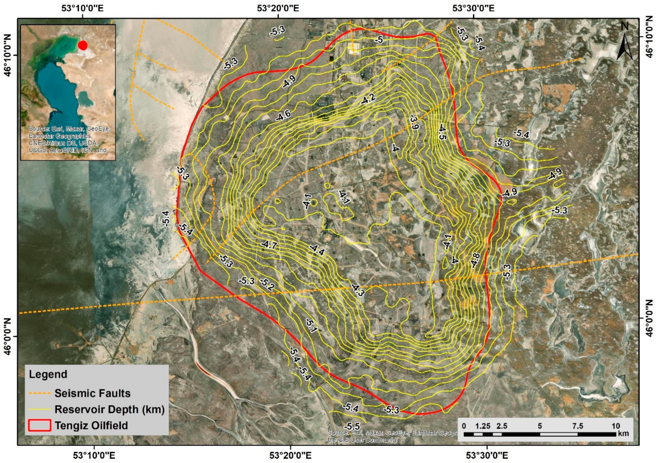
The development of the Tengiz oilfield started in 1991. It is located on the northern–eastern coast of the Caspian Sea and has an area of 2500 km
2. It covers 19 km in length and 21 km in width (
Figure 1). It is known as one of the largest and deepest carbonate oilfields in Kazakhstan, and it has an extensive natural fracture network and over 100 drilled wells [
27,
28]. As presented in
Figure 1, the Tengiz oilfield is crossed by faults which may always be subject to activation [
29]. According to Grebby et al. [
12], the estimated reservoir resources are 25.5 billion oil barrels within depths of 3.9–5.1 km. The current production rate is around 720,000 barrels per day. The top of the oil reservoir is located at a depth of about 4 km (
Figure 1). The terrain is flat with naturally formed depressions derived from snow and rainfall [
12]. The annual precipitation is 158 mm, and the annual air temperature is 11 °C. The climate is semi-arid with temperatures of −30 °C in the winter and 40 °C in the summer.
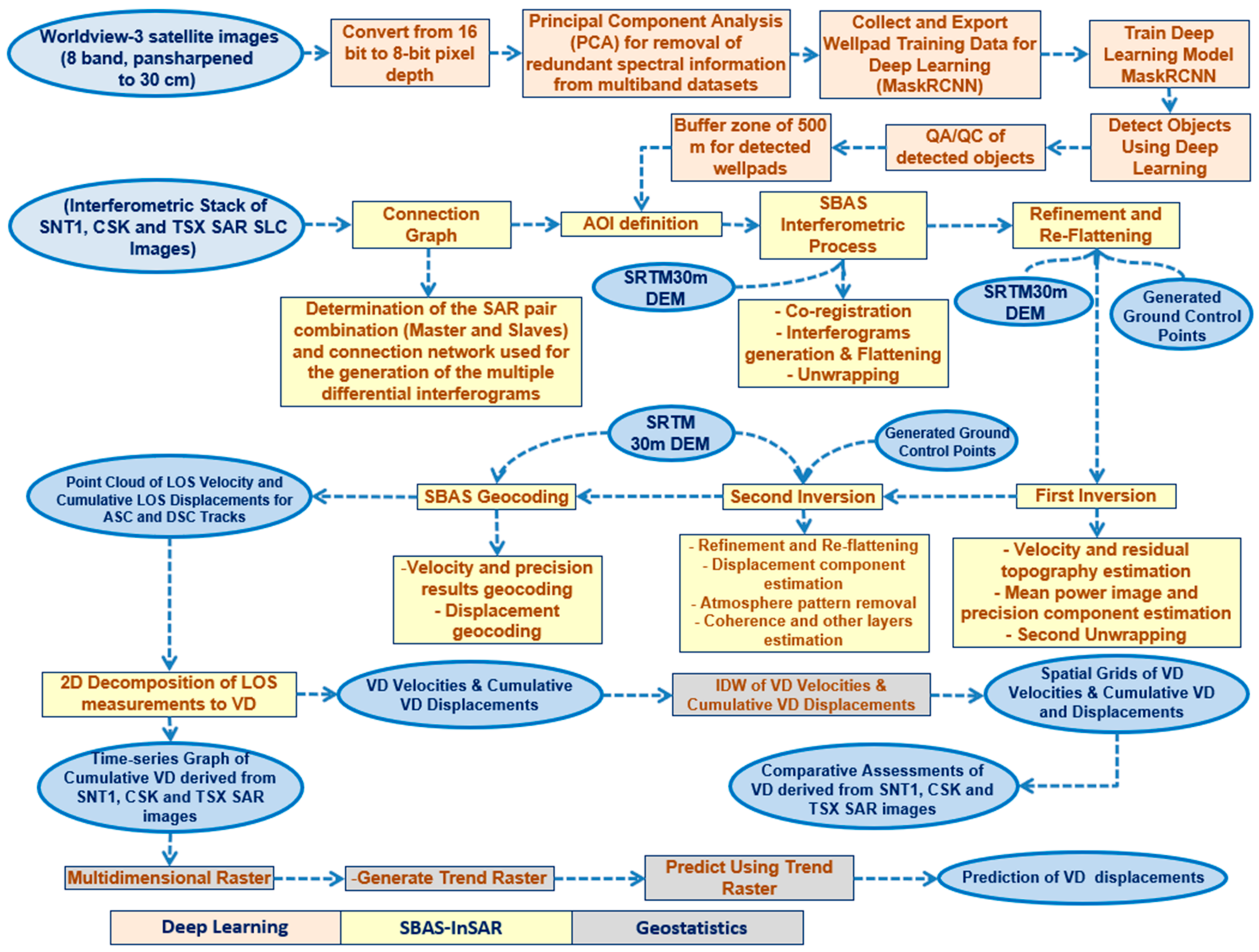
2.2. Deep Learning for the Recognition of Oil Wells, SBAS-InSAR Processing of CSK, TSX, and SNT1 SAR Images, and Geostatistical Analyses
For the remote sensing-based recognition of oil wells, pansharpened 0.3 m images from the Worldview-3 satellite mission were used to perform deep learning analyses (
Table 1). The pansharpenning was performed to achieve a better representation of wellpad boundaries. For the optimization of image processing speed, it was critical to reduce the size of the pansharpened images using two main techniques: the conversion of pixel depth from 16 bit to 8 bit and the Principal Component Analysis (PCA) of 16 spectral bands. The total size of the produced image was 600 megabytes. Both methods allowed for us to reduce the redundancy of information that would not improve the quality of our deep learning analyses and only serve to increase the processing speed. A mask region-based convolutional neural network (R-CNN) deep learning model was used for object detection and instance segmentation to precisely delineate the wellpad boundaries. Mask R-CNN, developed based on Faster R-CNN, is a state-of-the-art model for instance segmentation that generates bounding boxes for detected objects. The Mask R-CNN deep learning model was trained using 174 polygons of wellpads in the Tengiz oilfield to produce image chips (
Figure 2,
Figure 3 and
Figure 4). The parameters used to export the 174 training samples to chips and for the training of the deep learning model are presented in
Table 2. The validation of the trained model was performed based on the analyses of training and validation loss over epochs. The validation of detected objects was performed against ground reference data or training data using the following accuracy metrics: precision, recall, F1_Score, The Average Precision (AP) metric, true positive, false positive, and false negative (
Table 3). Moreover, additional validation was performed by visually inspecting each well and comparing them with the training samples.
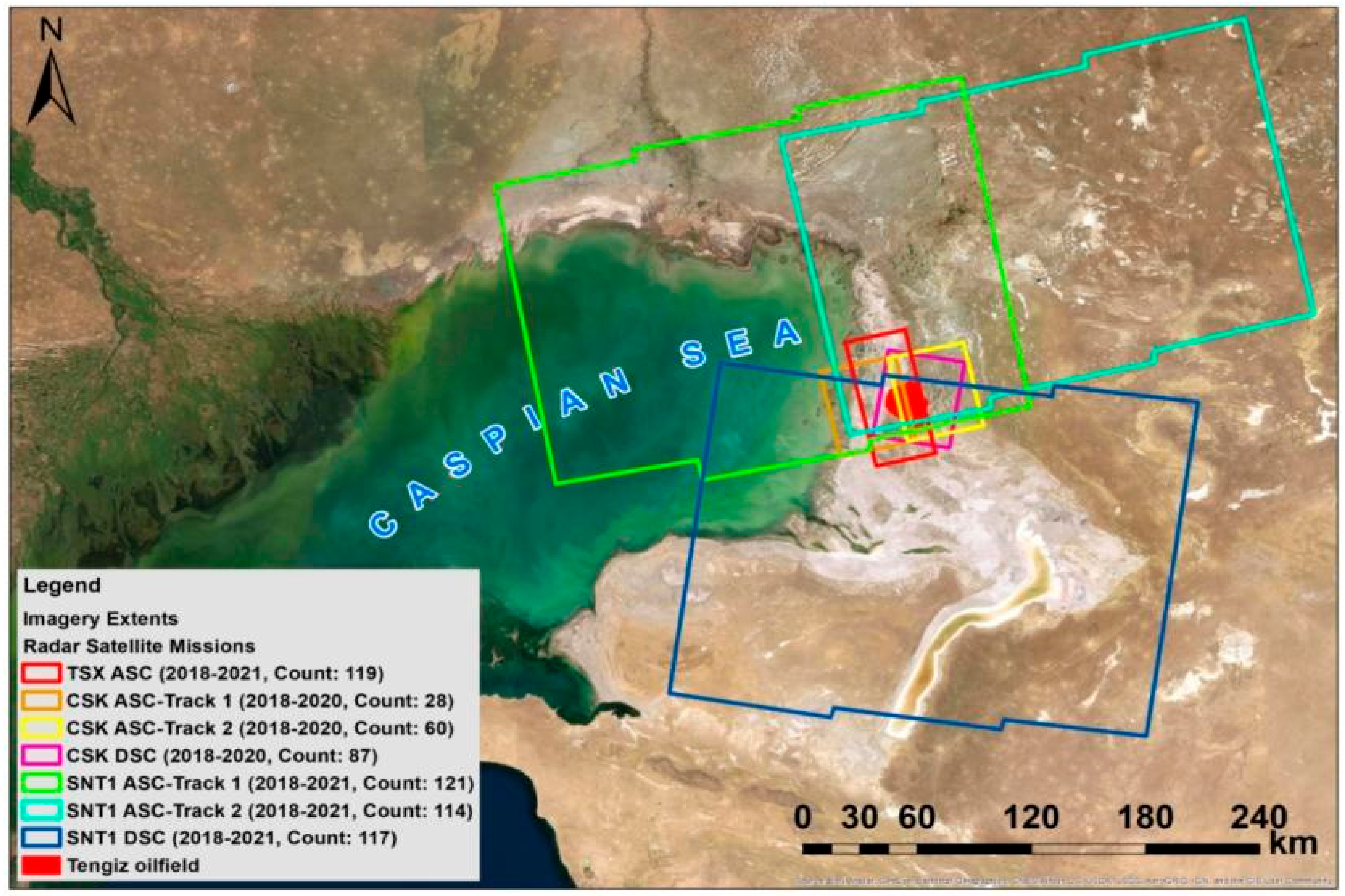
For the interferometric measurements, we used 96 descending and 235 ascending SNT1 SAR images from the European Space Agency (ESA), 119 TSX ascending SAR images from the German Aerospace Agency (DLR), and 87 descending and 88 CSK ascending SAR images from the Italian Space Agency (ASI). As presented in
Table 2, the CSK and TSX radar images were considered as high-resolution images with a spatial resolution of 3 m, whereas the SNT1 images were considered to have a medium resolution of 5 m by 20 m. The TSX and CSK SAR images were accessible in horizontal–horizontal (HH) polarization, while the SNT1 images were in vertical–vertical (VV) polarization. Both polarizations were verified as suitable for interferometric measurements and shown to contribute higher coherence and scattering [
33,
34,
35]. The detailed characteristics of the SAR images are presented in
Table 4. The ascending and descending footprints and counts of the CSK, SNT1, and TSX images are presented in
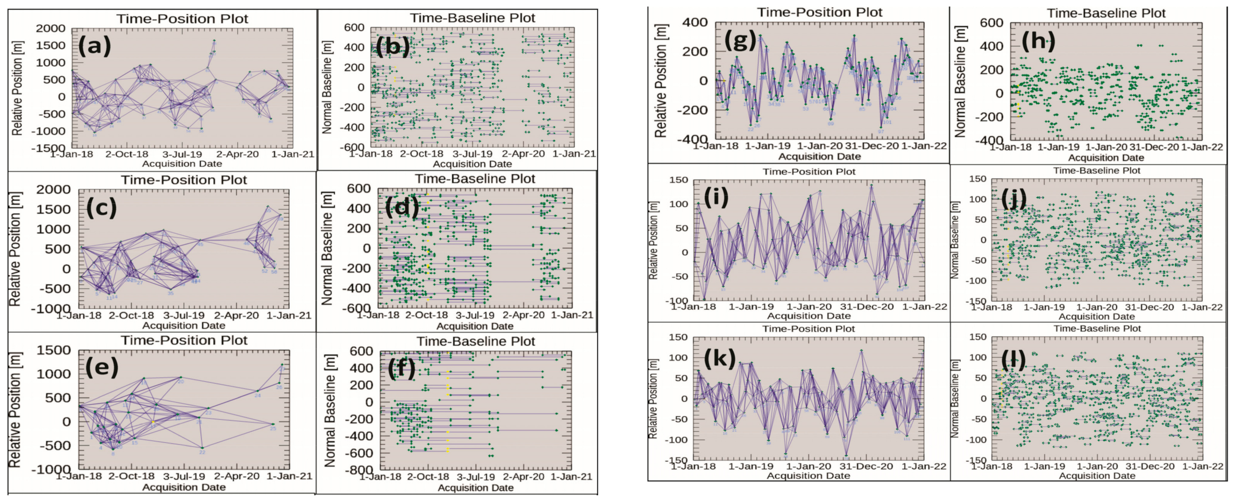
Figure 5. The connection graphs of the CSK, TSX, and SNT1 images in
Figure 6a–l show that all the SAR images were well connected in time for interferometric processing. TSX images were only acquired from the descending track.
The SBAS-InSAR technique was used for the displacement measurements [
38,
39,
40]. This technique is able to measure deformations for low-urbanized and low-vegetated areas, like the Tengiz oilfield, with weak temporal coherence. For the minimization of temporal decorrelations, optimal pairs of images were selected to reduce the spatial and temporal baselines [
38,
39,
40,
41,
42,
43,
44,
45].
The
Connection Graph step was performed to reduce the geometrical, temporal decorrelation for interferometric processing. The
SBAS-InSAR Interferometric Process allowed for us to generate interferograms for the ascending and descending tracks of the CSK, SNT1, and TSX images. The
Refinement and Re-flattening step allowed us to refine and re-flatten unwrapped interferometric phases using the polynomial method and ground control points [
46,
47,
48]. The
First Inversion step was performed to flatten the complex interferograms by re-calculating the phase unwrapping. The
Second Inversion was used to remove atmospheric phase components. The
SBAS Geocoding step was performed for the georeferencing of measured line-of-sight (LOS) velocities and displacements. Since InSAR measures displacements along the LOS direction, for the computation of vertical displacements, DSC and ASC tracks were decomposed along the vertical and horizontal directions using Equation (1) [
49,
50,
51,
52,
53,
54,
55,
56].
Since TSX data were only acquired from DSC track, this dataset was decomposed with the LOS measurements derived from the CSK ASC dataset, which has the same wavelength and spatial resolution (
Table 2).
where
asc and
dsc are the local incidence angles, and
asc and
dsc are the satellite heading angles of the ASC and DSC modes [
57]. In the present study, we only used vertical displacements.
For the geostatistical analysis, vertical displacement velocities and cumulative displacements derived from the CSK, TSX, and SNT1 satellite images were interpolated using the Inverse Distance Weighting (IDW) interpolation method. This geostatistical interpolation method was crucial for obtaining a more comprehensive interpretation of the produced results, geospatial analytics, and the prediction of deformation trends. ENVI SARscape software version 5.6.2 (Sarmap SA, Via Stazione 52, 6987 Caslano, Switzerland) was used for the interferometric processing of the TSX, CSK, and SNT1 SAR images using the SBAS-InSAR technique. ArcGIS Pro 3.2 software from Environmental Systems Research Institute (ESRI) was used for our deep learning analyses to detect wellpads. The workflow for the recognition of wellpads using deep learning, as well as that for obtaining interferometric measurements using SBAS-InSAR and geospatial analytics, is presented in
Figure 7.
3. Results
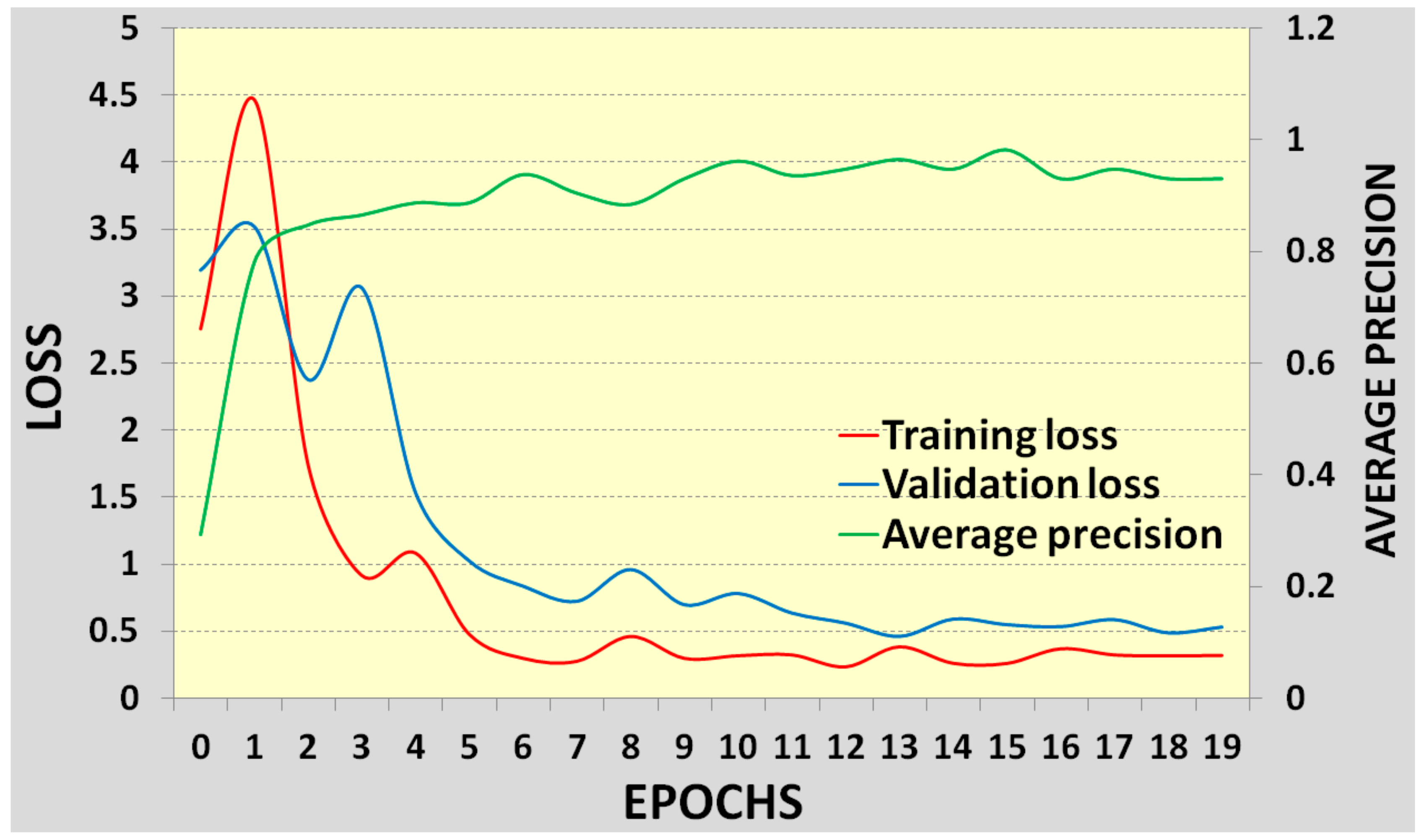
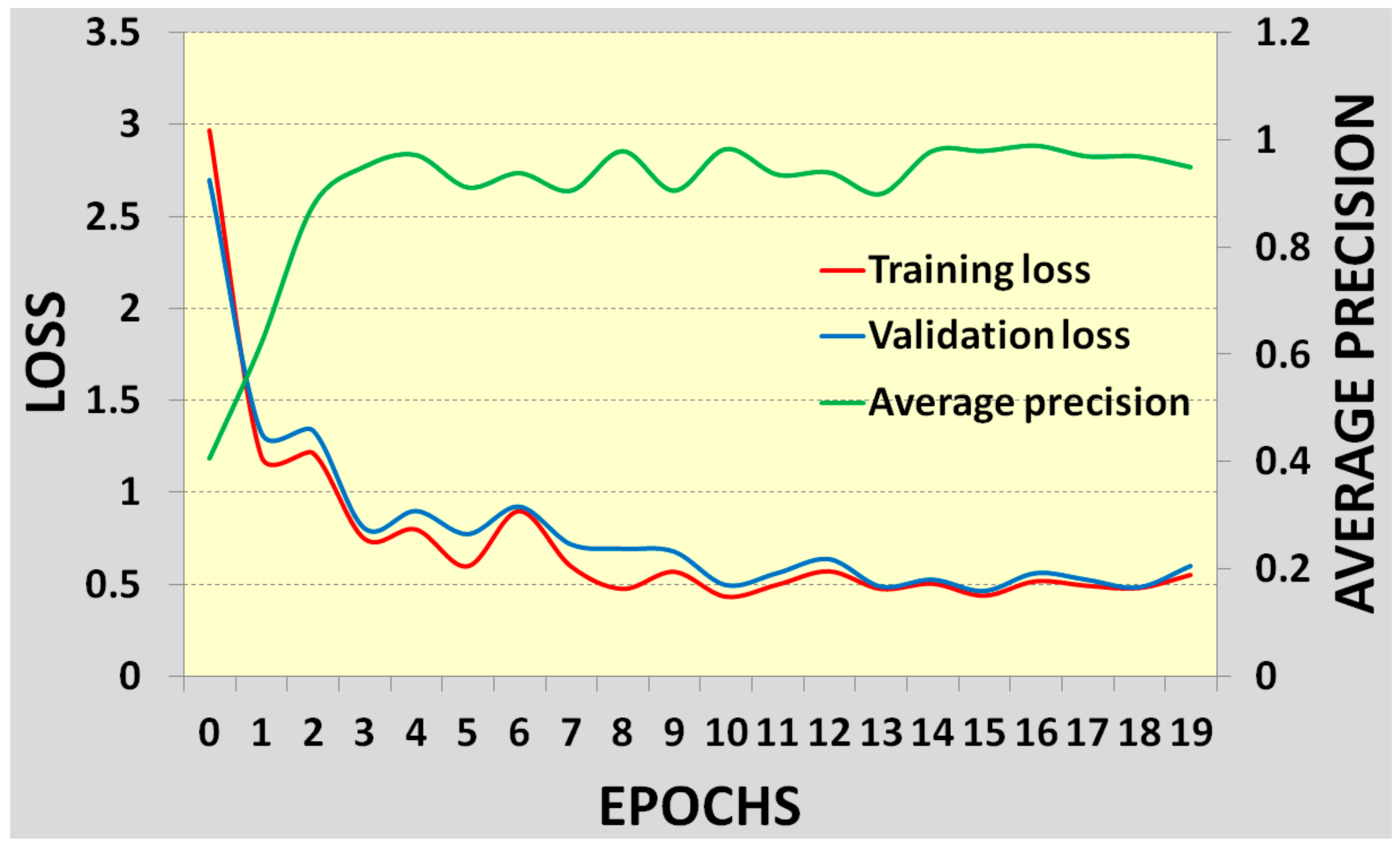
The training of the Mask R-CNN model using RGB images of 0.3 m and 1.24 m spatial resolutions showed different results in terms of fit between the training and validation loss curves. As shown in in
Figure 8, it was possible to observe that the lowering of training loss over epochs indicated a moderate fit with the training data, whereas the validation loss indicated some overfitting for the 1.24 m resolution RGB images. Regarding the pansharpened 0.3 m RGB images, the lowering of training loss over epochs indicated a good fit with the training data (
Figure 9). In both cases, The Average Precision score was observed to be in the range of 0.88. However, it was decided to proceed with the pansharpened RGB images because of their higher potential and reliability for object detection and obviously more accurate delineation of wellpad boundaries. It is necessary to emphasize the limitation of using this type of image: lower processing speed because of the higher spatial resolution.
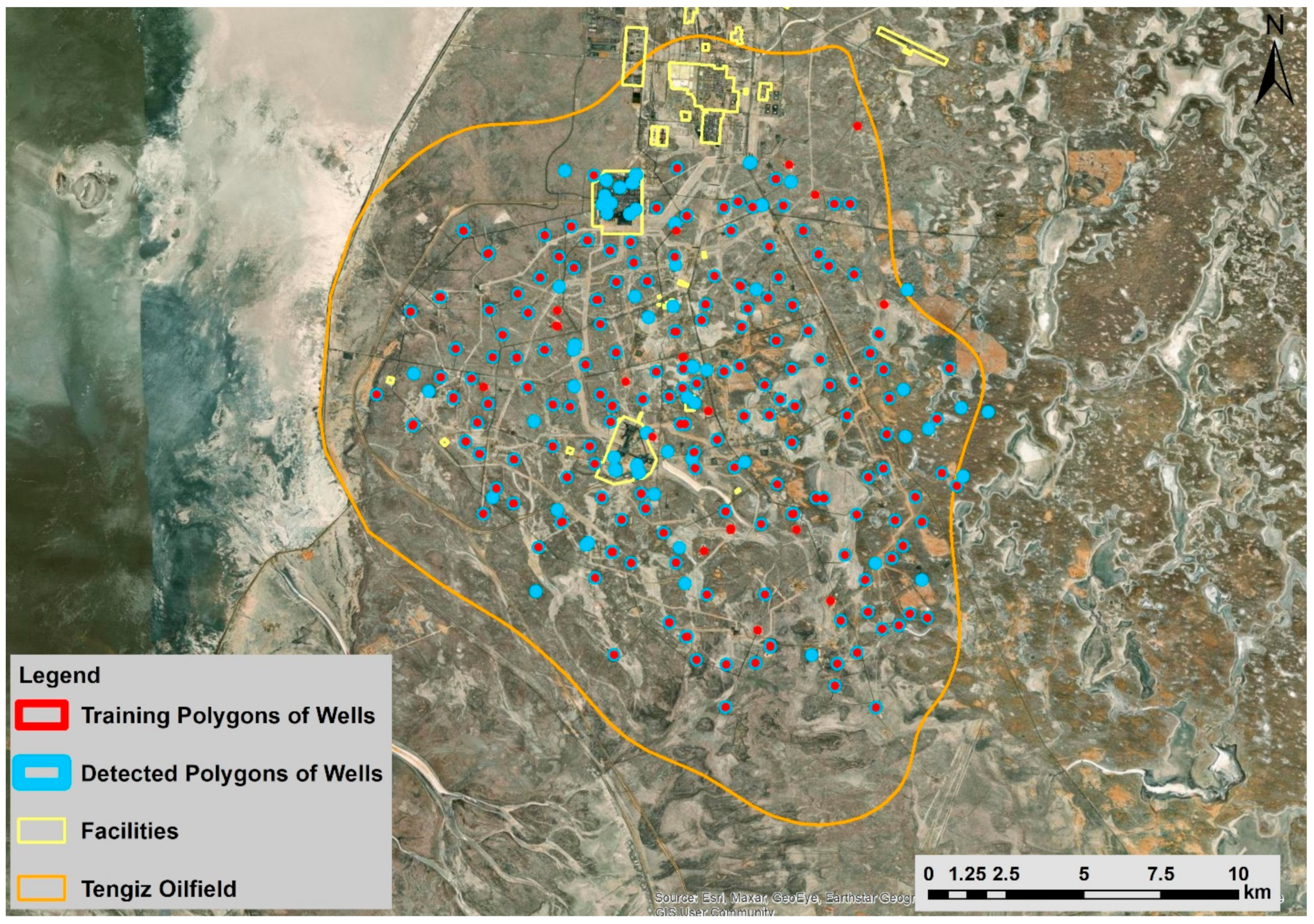
As a result of Mask R-CNN object detection processing, it was possible to detect 159 wells out of 174 with a confidence level of more than 95% (
Figure 10,
Table 5). The overlay analyses of the training and detected data of the wells showed that most of the wrongly detected wells (20) were located within oil terminals (
Figure 9). The precision, which is considered as the ratio of the number of true positives (159) to the total number of positive predictions (223), was observed to be 0.71 (
Table 5). The recall, considered as the ratio of the number of true positives (159) to the total number of actual (relevant) objects (174), was observed to be 0.91 (
Table 5). The F1_Score, considered as the weighted average of the precision and recall, was observed to be 0.80 (
Table 5). The Average Precision, considered as the precision averages across all recall values, was observed to be 0.77 (
Table 5).
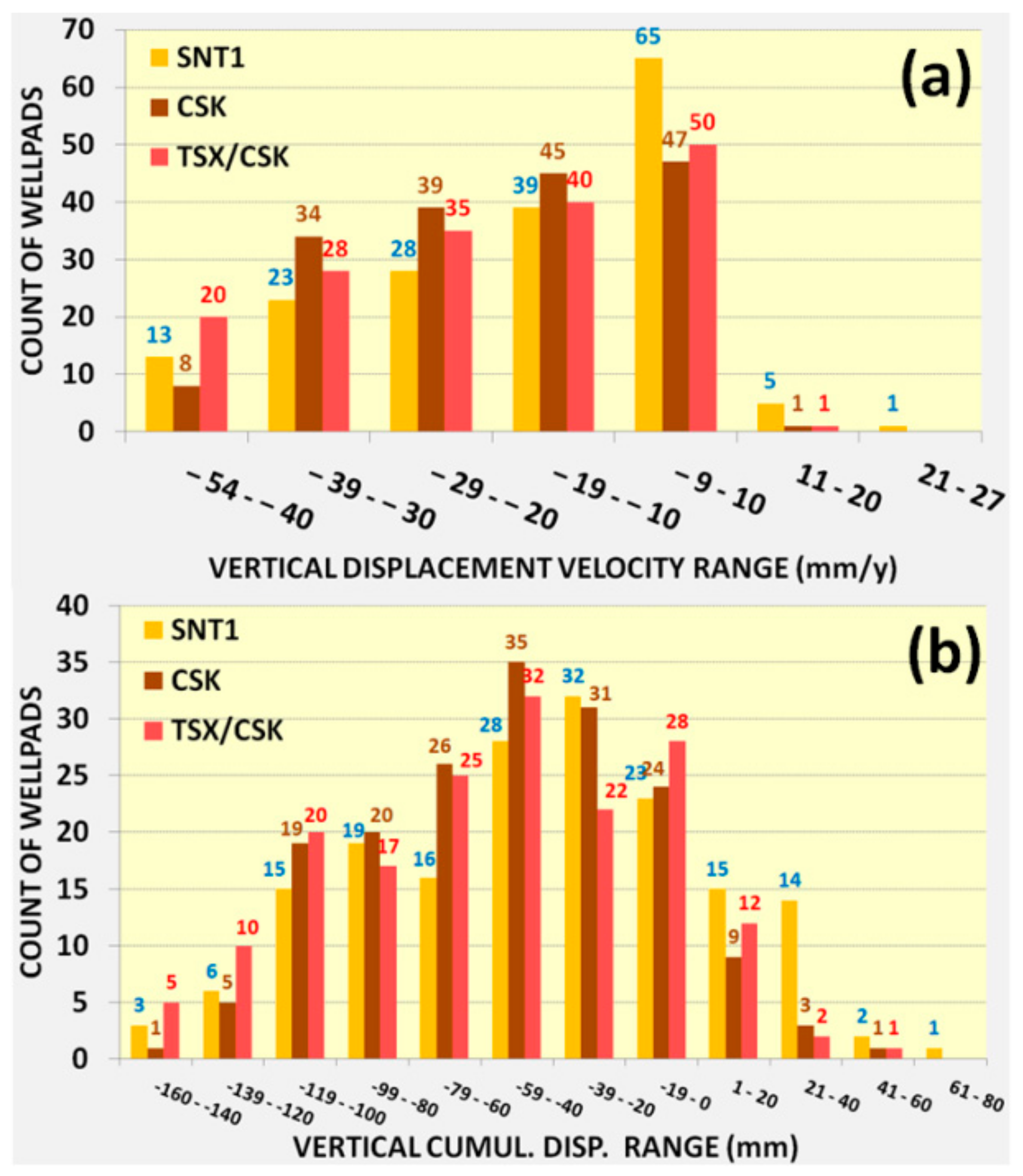
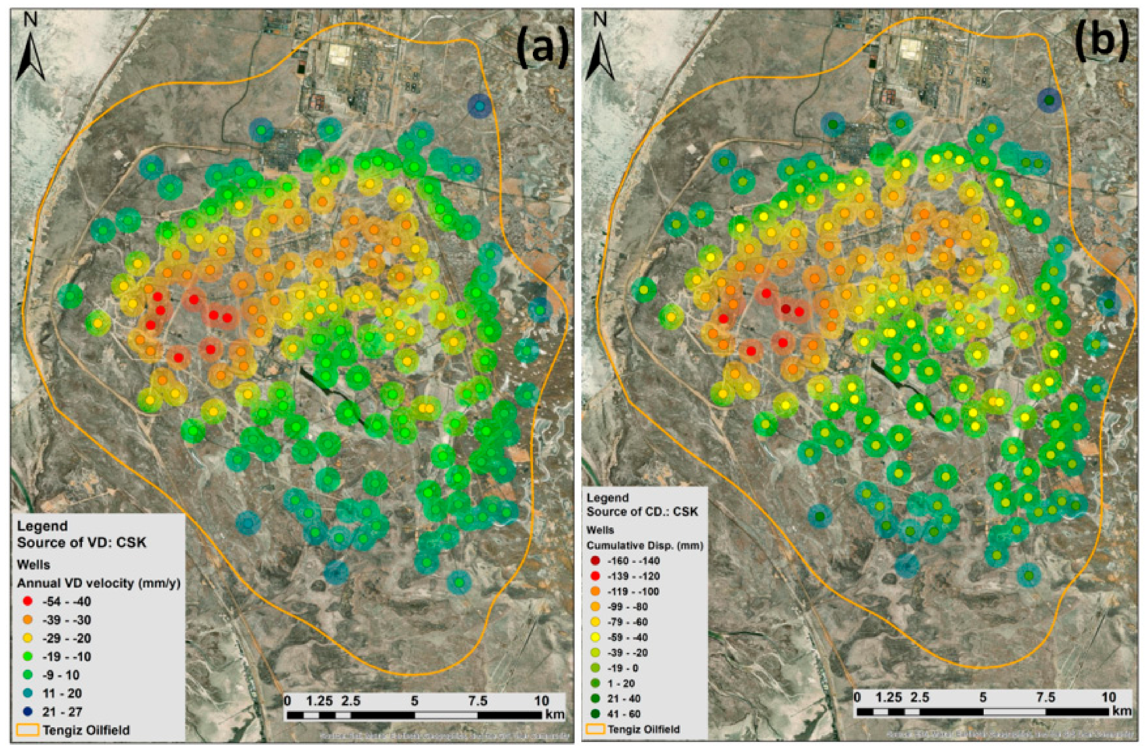
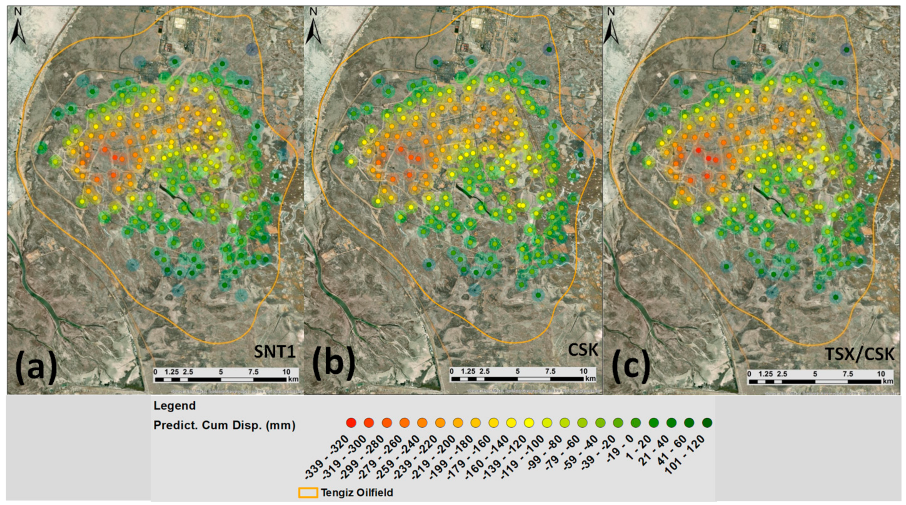
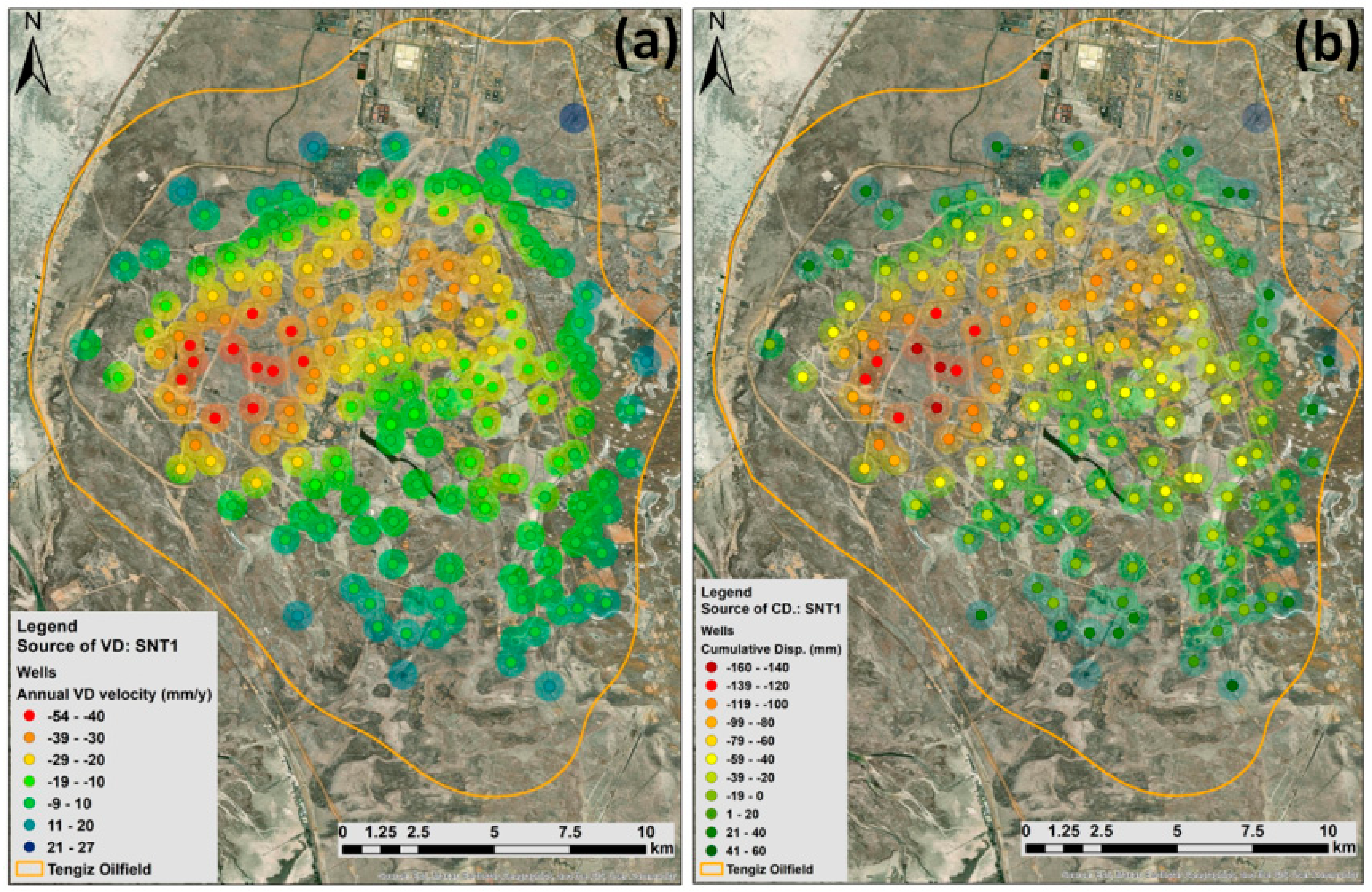
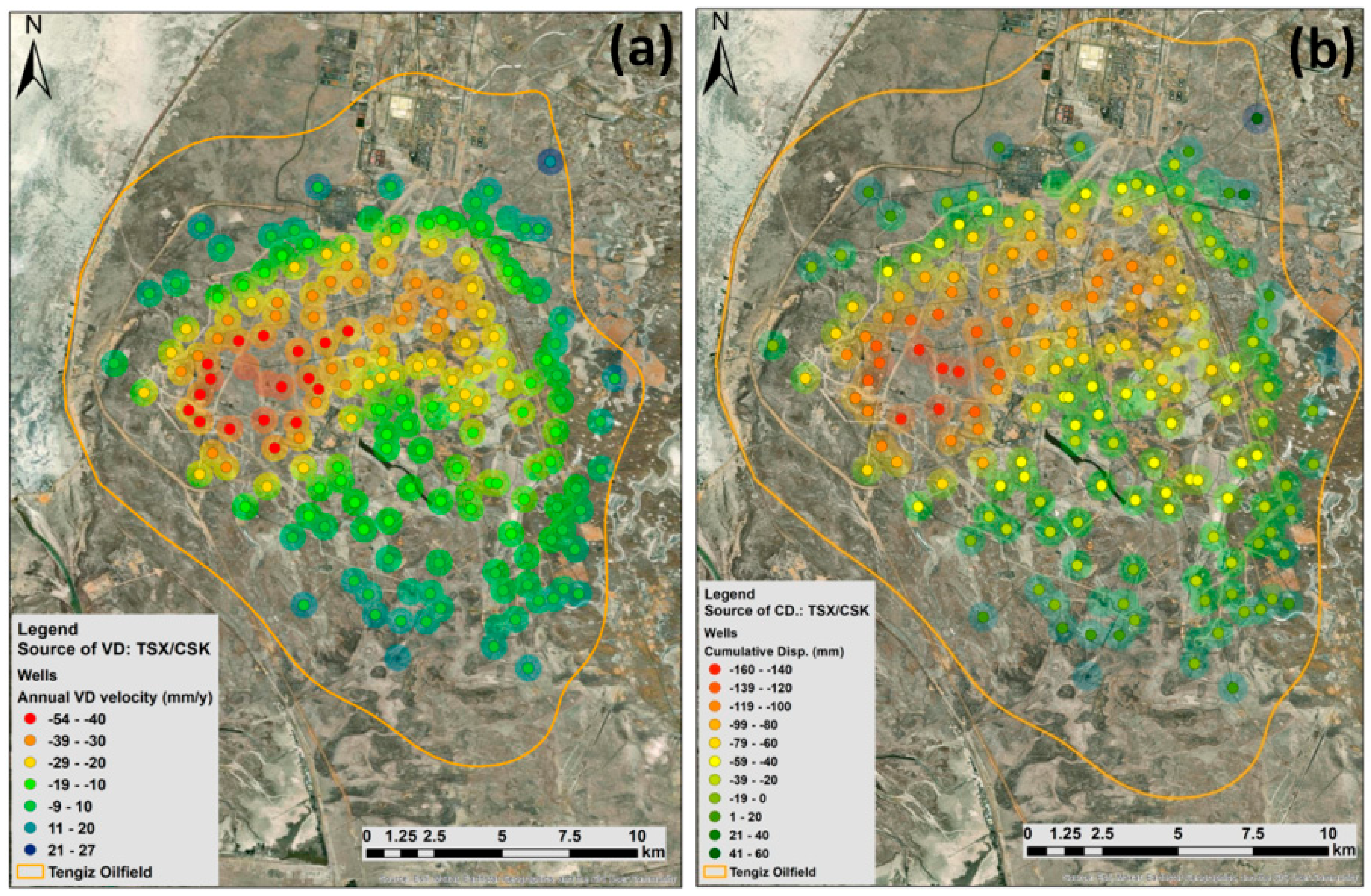
The SBAS-InSAR interferometric measurements identified 13 wells for SNT1, 8 wells for CSK, and 20 wells for TSX/CSK located within −54–−40 mm/y class of vertical displacement velocity (
Figure 11a;
Table 6). For the cumulative displacement of −139–−120 and −160–−140, the summarized number of identified wells was 9 for SNT1, 6 for CSK, and 15 for TSX/CSK (
Figure 11b;
Table 6). These wells are indicated in a reddish color in
Figure 12,
Figure 13 and
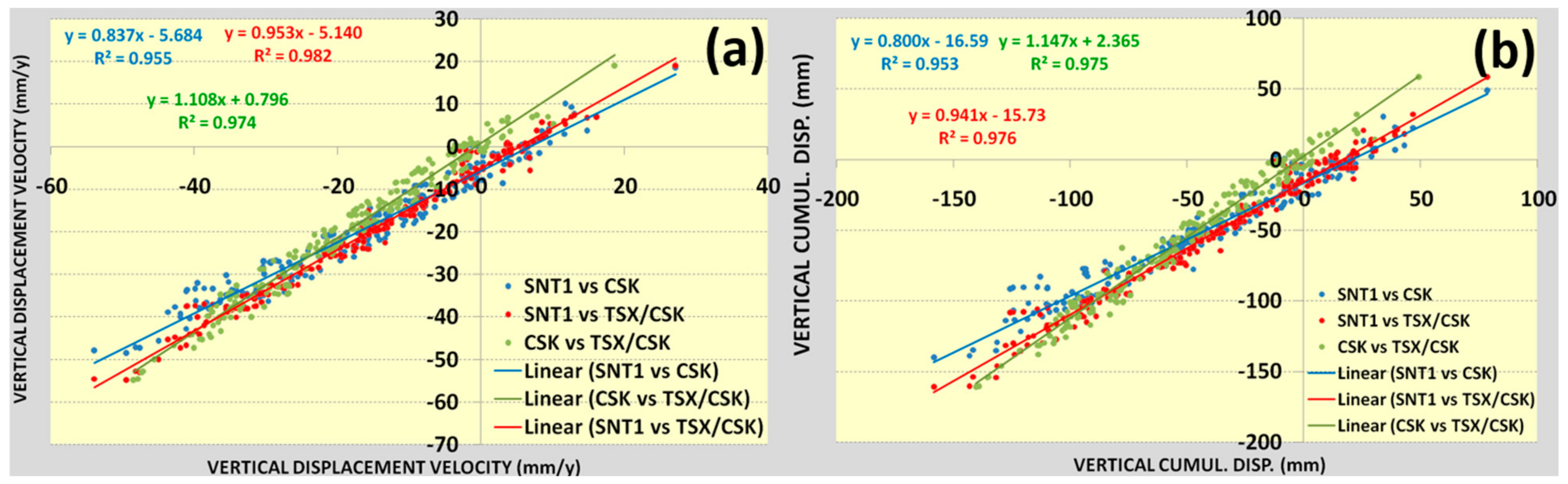
Figure 14a,b. As it is possible to observe, wells of higher subsidence vulnerability are located close to each other, being mainly concentrated in the north–west of the Tengiz oilfield. This means that oil extraction and injection activities are not rationally distributed over the Tengiz oilfield. However, there was no accessible and specified engineering standard that we could use to make a judgement about the criticality of this subsidence. Even though SBAS-InSAR interferometric measurements from SNT1, CSK, and TSX/CSK images showed a strong agreement with R
2 > 0.95, it is necessary to emphasize that on the level of each wellpad, the subsidence and uplift values differed for different satellite missions (
Figure 15a,b). This fact could certainly create uncertainty for oil and gas operators in risk assessment and decision making. The authors of the present study did not have access to ground GPS or leveling measurements; therefore, it was complicated to ascertain the accuracy of the measurements derived from the three satellites, but it was possible to confirm that the overall deformations were correctly measured from all three satellite missions with spatially identical subsidence and uplift patterns. In addition, it was also possible to clearly observe that the combination of TSX and CSK SBAS-InSAR measurements showed higher subsidence rates.
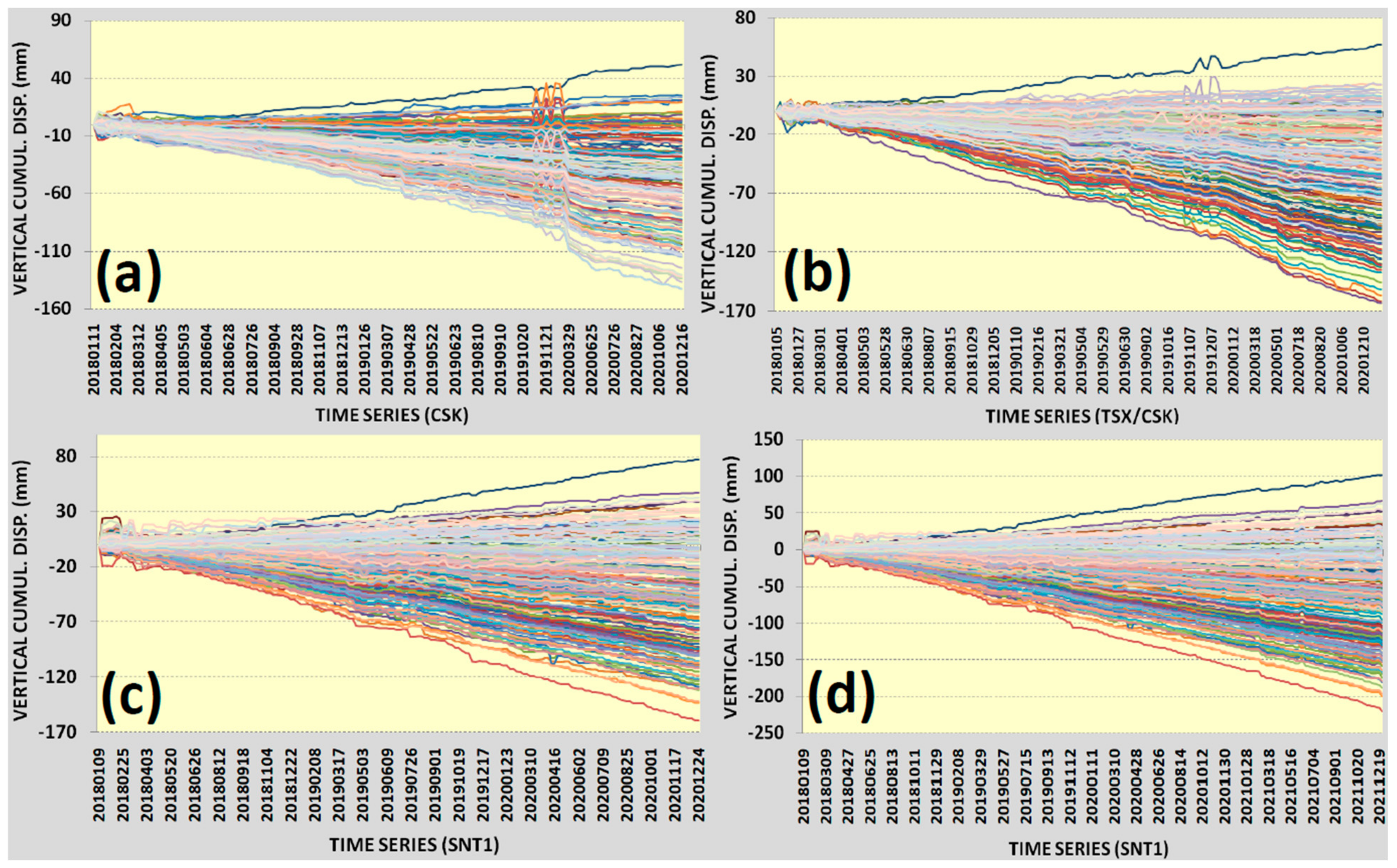
As mentioned before, regression analyses for the annual deformation velocities and cumulative displacements of wells derived from SNT1, CSK, and TSX satellite missions showed a good agreement with R
2 > 95. Hence, both the medium- and high-resolution satellite missions showed identical results (
Figure 15a,b). Based on
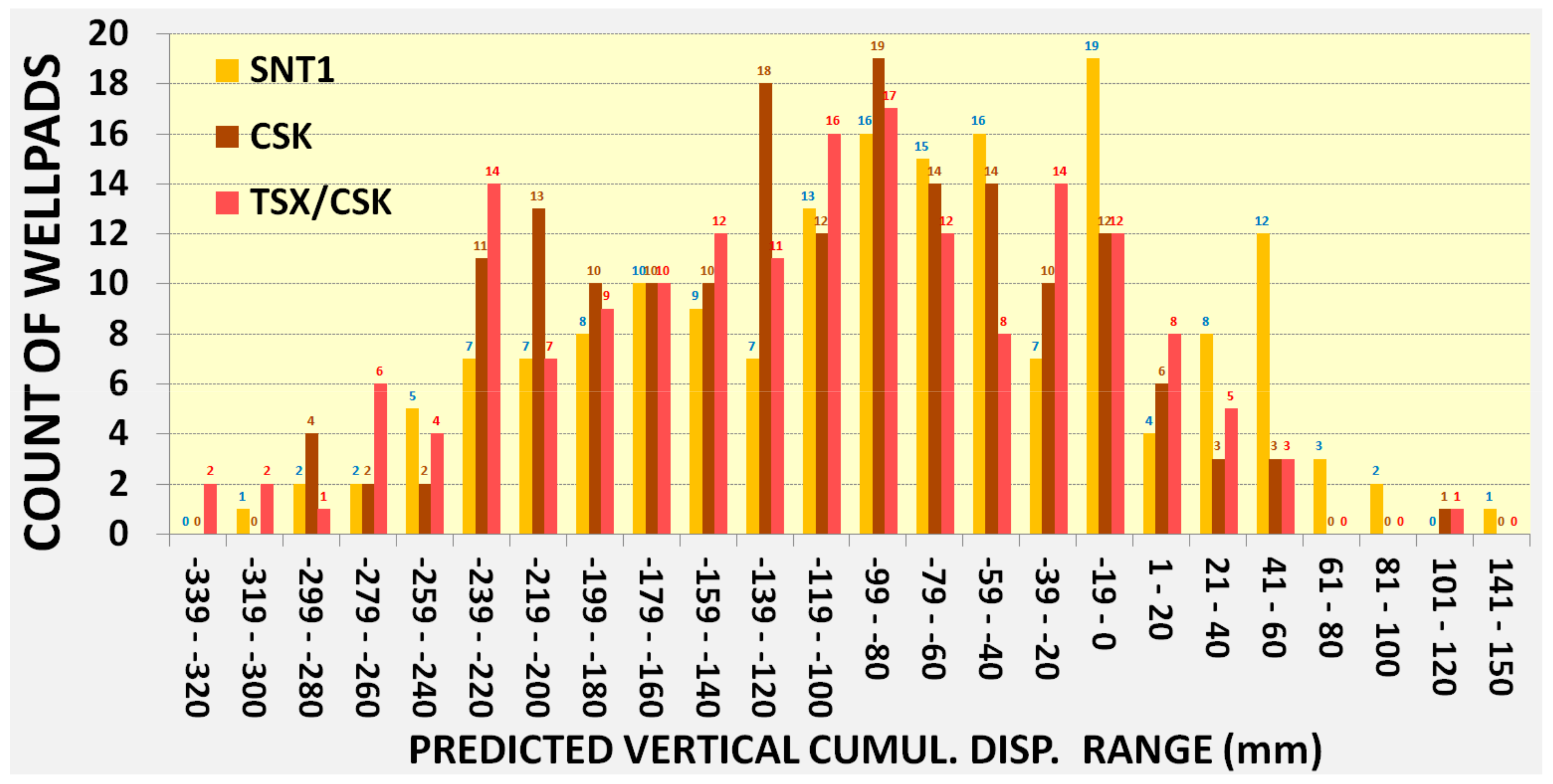
Figure 16a–c, it was possible to observe that apart from subsidence, some wells were also affected by uplift processes. The cumulative displacement reached −160 mm for SNT1 (24 December 2020), −142 mm for CSK (16 December 2020), and −163 for TSX/CSK (10 December 2020). Since SNT1 images were also available till 30 December 2021, it was possible to observe that the subsidence processes continued and reached −220 mm (30 December 2021). This means that the trend of subsidence processes continues with the same spatial deformation patterns. The predictions for cumulative displacements showed that the vertical subsidence processes will continue and reach −339 mm on 31 December 2023, with increasing spatial coverage and the potential to impact a higher number of wells (
Figure 17a–c and
Figure 18;
Table 7).
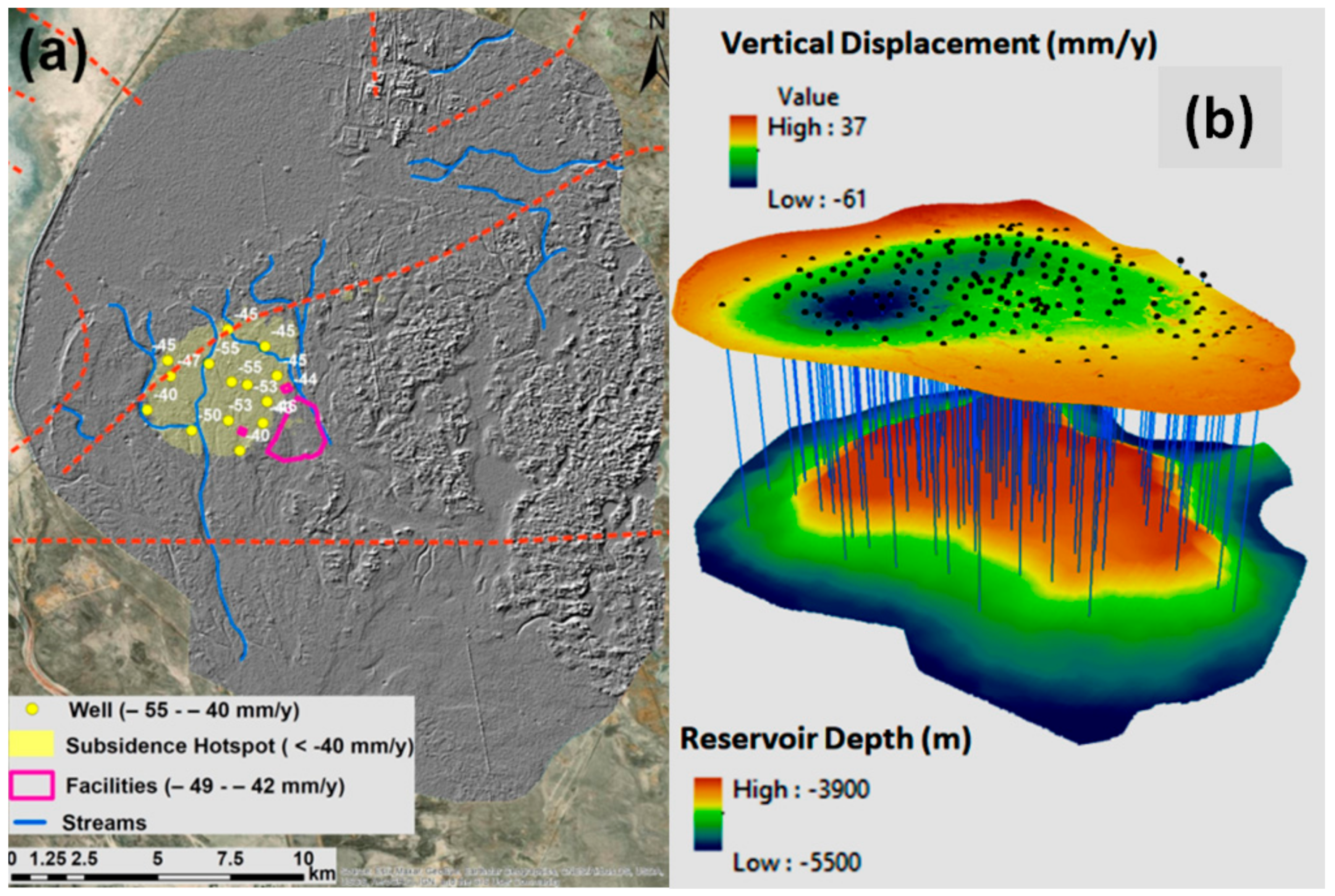
The hydrological analyses in the Tengiz oilfield clearly demonstrated that water flow has been moving towards a subsidence hotspot (
Figure 19a). Thus, water accumulation will also be increasing in the continuously subsiding hotspot. This detected subsidence hotspot was observed at a crossing with a seismic fault that might always be subject to reactivation (
Figure 19a). The role of this seismic fault should also be investigated as one of the ground deformation-controlling factors, even though this area is not considered seismically active. Based on
Figure 19b, which shows the shape and depth of the subsurface of the reservoir, it was possible to observe that major subsidence trends move towards the edge of this reservoir.
4. Discussion
In this study, we have demonstrated the reliability of our wellpad recognition approach, which achieved a precision value of 0.71 and a recall value of 0.91. It was possible to detect 159 wells out of 174 with a confidence level of more than 95%. Most of the false-positive or wrongly detected wells were located within oilfield facilities and had to be cleaned manually. This allowed us to prioritize areas of primary interest for the subsequent targeted interferometric measurements of vertical displacements. These studies also demonstrated that the use of high-resolution optical images for the recognition of wellpads and subsequent targeted interferometric measurements for the optimal buffer zones of these wellpads, together, could significantly optimize operational monitoring and risk assessment activities in the Tengiz oilfield. Our comparative analyses of InSAR measurements using CSK, TSX, and SNT1 satellite missions showed good agreement with R2 > 95 for vertical displacement velocities. It is possible to conclude that the Tengiz oilfield operator could use either of these sensors or also consider using medium-resolution SNT1 satellite images for operational cost saving. Besides the fact that the interferometric measurements from three satellite missions provided identical results, they also allowed us to validate the reliability of the vertical displacement measurements for the Tengiz oilfield. Since we did not have any access to in situ geodetic measurements, this method was prioritized to verify the quality of the measurements. The SBAS-InSAR interferometric measurements identified 13 wells for SNT1, 8 wells for CSK, and 20 wells for TSX/CSK located within −54–−40 mm/y class of vertical displacement velocity. For the cumulative displacement of −139–−120 and −160–−140, the summarized number of identified wells was 9 for SNT1, 6 for CSK, and 15 for TSX/CSK. Even though the number of wells varied within the different vertical displacement classes, these variations were in the range of 5–10 mm. The predictions for cumulative displacements showed that the vertical subsidence processes will continue and reach −339 mm on 31 December 2023, with increasing spatial coverage and the potential to impact a higher number of wells. The hydrological analyses in the Tengiz oilfield clearly demonstrated that water flow has been moving towards a subsidence hotspot. Thus, water accumulation will also increase in the continuously subsiding hotspot. It is necessary to emphasize that the increasing accumulation of water could potentially affect subsidence acceleration and the corrosion levels of existing facilities as well.
The studies by Wang et al. [
20] and Giri et al. [
21] presented identical precision and recall values with our results but for Faster RCNN, SSD, and RetinaNet deep learning models. The primary difference between these studies and ours is that these models generated bounding boxes for wellpads, whereas Mask R-CNN generated actual boundaries of wellpads through the instance segmentation technique, which performed pixel-level segmentation on detected wellpads. We also compared our results with previous studies and determined the consistency of our results showing a continuous subsidence process in the Tengiz oilfield [
9,
11,
12,
13,
14,
15]. Based on the work of Bayramov et al. [
15], regarding SBAS-InSAR processing times, around one month was needed for a satellite image of the entire Tengiz oilfield. In the present study, we managed to decrease the processing time to three days by targeting detected wellpads which were of primary interest to optimize operational monitoring and risk assessment timing for oil and gas operators to mitigate possible geohazard risks.
As for the shortcomings of the Mask R-CNN model, it is necessary to emphasize that most of the false-positive wellpads were located within oilfield facilities. This means that the introducing these facilities to a different class during the training data collection and model training would support the model in separating them from wellpads. The same is relevant to some wellpads with a changed standard pattern which were abandoned or in the process of construction. They also created some confusion for the model, and it would also be reasonable to separate them into a different class. It was also mentioned in the referenced study by Giri et al. [
21] that by grouping the false positives together into different categories for use as target classes for training, one can expect the model to learn the differences among the classes during the model training process. This would contribute to significantly reducing false positives. As for the shortcomings of the SBAS-InSAR interferometric measurements, it is important to emphasize that our measurements are differential relative to the reference point, and we can only judge the period of 2018–2020. This means that we could not be aware of what was going on in terms of ground deformations before this period since historical GPS ground measurements were not accessible. Another limitation is a lack of in situ geodetic measurements for the validation of interferometric measurements. For future root cause analyses of natural seismic and flooding factors and man-made oil extraction activities, it is highly important to have subsurface seismic data and time-series of production information. In addition, it is recommended to regularly perform field observations of wells located within the detected subsidence hotspot to look for any possible damage. Established engineering standards were not accessible for the present study, hindering our ability to determine what level of displacement is considered sensitive to wells; therefore, it is difficult to state anything about the criticality of detected displacements, but it is possible to state that the subsidence will continue to increase unless proper measures are taken in time. In addition, we should not dismiss the fact that some of the wells are also affected by the uplift processes which occur around the Tengiz oilfield. This should also be investigated in the future. The studies by Tamburini et al. [
58], Brew et al. [
59], and Leezenberg et al. [
60] related the role of InSAR measurements to the depth of a petroleum reservoir. In the present study, it was complicated to determine a direct relationship between oil extraction activities and the detected subsidence hotspot since we did not have any geological and geophysical subsurface and production-related data from the oilfield located at a depth of −3900 m. However, according to Nagel et al. [
61], the existence of oil reservoir deformation demonstrated its dynamic behavior in terms of reservoir compaction, uplift, and subsidence, which could affect oil production and recovery both negatively and positively. Therefore, the present study could play a significant role for reservoir characterizations and be an important resource for researchers aiming to carry out reservoir modeling to determine regular correlations between ground displacements and production rates. Additionally, this study could contribute to the planning of future injections, specifically with respect to ensuring their correct positioning, and production wells to mitigate the risks of continuous subsidence and strengthen the foundations of existing wells.
5. Conclusions
The Mask R-CNN model has been shown to be capable of detecting wellpads from satellite images with different shapes, orientations, and sizes. In the present study, the Mask R-CNN model reached a precision value of 0.71 and a recall value of 0.91. It was possible to detect 159 wells out of 174 with a confidence level of more than 95%. The model would perform better with the inclusion of oilfield facilities in a separate category of training samples since most of the false-positive wellpads were located there. Additionally, we also recommend the inclusion of abandoned or under-construction wellpads with lost wellpad patterns in a separate category since they also created a confusion for the trained model. Grouping the false positives together into different categories as target classes for training would benefit the model by allowing it to learn the differences among the classes during the model training process and, subsequently, carry out detection with reduced false positives.
Regression analyses for the annual deformation velocities and cumulative displacements of wells derived from SNT1, CSK, and TSX satellite missions showed a good agreement with R2 > 95. Hence, both the medium- and high-resolution satellite missions showed identical results. This means that operators of oil and gas fields could also apply freely accessible medium-resolution radar images for operational cost saving. The SBAS-InSAR interferometric measurements identified 13 wells for SNT1, 8 wells for CSK, and 20 wells for TSX/CSK located within −54–−40 mm/y class of vertical displacement velocity. For the cumulative displacement of −139–−120 and −160–−140, the summarized number of identified wells was 9 for SNT1, 6 for CSK, and 15 for TSX/CSK. Apart from subsidence, some wells were affected by uplift processes towards the boundaries of the Tengiz oilfield. The predictions for cumulative displacements showed that the vertical subsidence processes will continue and reach −339 mm on 31 December 2023, with increasing spatial coverage and the potential to impact a higher number of wells. The hydrological analyses in the Tengiz oilfield clearly demonstrated that water flow has been moving towards a subsidence hotspot. This allowed us to conclude that water accumulation will also increase in the continuously subsiding hotspot. This detected subsidence hotspot was observed at a crossing with a seismic fault that might always be subject to reactivation. The role of this seismic fault should also be investigated as one of the ground deformation-controlling factors, even though this area is not considered seismically active.
Our future research goal is to improve the performance of the developed Mask R-CNN model by including more categories for the training samples and increasing the library of training samples of different wellpad types from various high-resolution satellite missions for all oil and gas fields located along the Caspian Sea. As for the InSAR measurements, we also plan to increase the temporal range of observations and try other techniques pertaining to interferometric measurements and radar satellite missions.
Author Contributions
Writing—original draft preparation: E.B. and S.A.; writing—review and editing: G.T., E.B. and A.D.; supervision: M.K.; resources: E.B. and S.A. All authors have read and agreed to the published version of the manuscript.
Funding
This study was funded by the Nazarbayev University through Faculty-development Competitive Research Grant (FDCRGP) (AI and Data Science) 2024–2026—Funder Project Reference: 201223FD2607, Collaborative Research Program 2024–2026—Funder Project Reference: 211123CRP1606, and the Social Policy Grant (201705).
Data Availability Statement
Data are contained within the article.
Acknowledgments
The authors would like to acknowledge Nazarbayev University. This study was funded by the Nazarbayev University through Faculty-development Competitive Research Grant (FDCRGP) (AI and Data Science) 2024–2026—Funder Project Reference: 201223FD2607, Collaborative Research Program 2024–2026—Funder Project Reference: 211123CRP1606, and the Social Policy Grant (201705). This project was carried out using COSMO-SkyMed images of ASI (Italian Space Agency), delivered under an ASI license to use in the framework of COSMO-SkyMed Open Call for Science Project ID 767. The authors would like to acknowledge the Italian Space Agency (Agenzia Spaziale Italiana) for their provision of COSMO-SkyMed (CSK) images within the Open Call for Science Project ID 767. The authors also kindly acknowledge the European Space Agency (ESA) for making available the Sentinel-1 images in the framework of Copernicus Programme.
Conflicts of Interest
Author Giulia Tessari was employed by the company Sarmap SA. The remaining authors declare that the research was conducted in the absence of any commercial or financial relationships that could be construed as a potential conflict of interest.
References
- Rabus, B.; Werner, C.; Wegmueller, U.; McCardle, A. Interferometric point target analysis of RADARSAT-1 data for deformation monitoring at the Belridge/Lost Hills oil fields’. In Proceedings of the Geoscience and Remote Sensing Symposium 2004 (IGARSS’04), Anchorage, AK, USA, 20–24 September 2004; Institute of Electrical and Electronics Engineers: Piscataway, NJ, USA, 2004; Volume 4, pp. 2611–2613. [Google Scholar]
- Zhou, W.; Chen, G.; Li, S.; Ke, J. InSAR Application in Detection of Oilfield Subsidence on Alaska North Slope. In Proceedings of the 41st US Symposium on Rock Mechanics (USRMS), Golden, CO, USA, 17–21 June 2006. [Google Scholar]
- Gee, D.; Sowter, A.; Novellino, A.; Marsh, S.; Gluyas, J. Monitoring land motion due to natural gas extraction: Validation of the Intermittent SBAS (ISBAS) DInSAR algorithm over gas fields of North Holland, The Netherlands. Mar. Pet. Geol. 2016, 77, 1338–1354. [Google Scholar] [CrossRef]
- Staniewicz, S.; Chen, J.; Lee, H.; Olson, J.; Savvaidis, A.; Reedy, R.; Breton, C.; Rathje, E.; Hennings, P. InSAR reveals complex surface deformation patterns over an 80,000 km2oil-producing region in the Permian Basin. Geophys. Res. Lett. 2020, 47, e2020GL090151. [Google Scholar] [CrossRef]
- Togaibekov, A.Z. Monitoring of Oil-Production-Induced Subsidence and Uplift. Master’s Thesis, Massachusetts Institute of Technology, Cambridge, MA, USA, 2020. [Google Scholar]
- Xu, Y. Analysis of common geological hazards in oil and gas fields. Heilongjiang Sci. Technol. Inf. 2014, 16, 71. [Google Scholar]
- Shi, J.; Yang, H.; Peng, J.; Wu, L.; Xu, B.; Liu, Y.; Zhao, B. InSAR Monitoring and analysis of ground deformation due to fluid or gas injection in Fengcheng oil field, Xinjiang, China. J. Indian Soc. Remote Sens. 2019, 47, 455–466. [Google Scholar] [CrossRef]
- Fokker, P.A.; Visser, K.; Peters, E.; Kunakbayeva, G.; Muntendam-Bos, A.G. Inversion of surface subsidence data to quantify reservoir compartmentalization: A field study. J. Pet. Sci. Eng. 2012, 96, 10–21. [Google Scholar] [CrossRef]
- Del Conte, S.; Tamburini, A.; Cespa, S.; Rucci, A.; Ferretti, A. Advanced InSAR Technology for Reservoir Monitoring and Geomechanical Model Calibration. In SPE Kuwait Oil and Gas Show and Conference; Society of Petroleum Engineers (SPE): Richardson, TX, USA, 2013. [Google Scholar] [CrossRef]
- Rocca, F.; Rucci, A.; Ferretti, A.; Bohane, A. Advanced InSAR interferometry for reservoir monitoring. First Break 2013, 31, 77–85. [Google Scholar] [CrossRef]
- Comola, F.; Janna, C.; Lovison, A.; Minini, M.; Tamburini, A.; Teatini, P. Efficient global optimization of reservoir geomechanical parameters based on synthetic aperture radar-derived ground displacements. Geophysics 2016, 81, M23–M33. [Google Scholar] [CrossRef]
- Grebby, S.; Orynbassarova, E.; Sowter, A.; Gee, D.; Athab, A. Delineating ground deformation over the Tengiz oil field, Kazakhstan, using the Intermittent SBAS (ISBAS) DInSAR algorithm. Int. J. Appl. Earth Obs. Geoinf. 2019, 81, 37–46. [Google Scholar] [CrossRef]
- Orynbassarova, E. Improvement of the Method of Integrated Preparation and Use of Space Images in Tasks of Assessment of Sedimentation of Industrial Surface in the Conditions of Operation of Tengiz Oil and Gas Field. Ph.D. Thesis, Satbayev University, Almaty, Kazakhstan, 2019. [Google Scholar]
- Bayramov, E.; Buchroithner, M.; Kada, M.; Zhuniskenov, Y. Quantitative Assessment of Vertical and Horizontal Deformations Derived by 3D and 2D Decompositions of InSAR Line-of-Sight Measurements to Supplement Industry Surveillance Programs in the Tengiz Oilfield (Kazakhstan). Remote. Sens. 2021, 13, 2579. [Google Scholar] [CrossRef]
- Bayramov, E.; Buchroithner, M.; Kada, M.; Duisenbiyev, A.; Zhuniskenov, Y. Multi-Temporal SAR Interferometry for Vertical Displacement Monitoring from Space of Tengiz Oil Reservoir Using SENTINEL-1 and COSMO-SKYMED Satellite Missions. Front. Environ. Sci. 2022, 10, 783351. [Google Scholar] [CrossRef]
- Ferretti, A.; Tamburini, A.; Novali, F.; Fumagalli, A.; Falorni, G.; Rucci, A. Impact of high resolutionradar imagery on reservoir monitoring. Energy Procedia 2011, 4, 3465–3471. [Google Scholar] [CrossRef]
- Even, M.; Westerhaus, M.; Simon, V. Complex Surface Displacements above the Storage Cavern Field at Epe, NW-Germany, Observed by Multi-Temporal SAR-Interferometry. Remote. Sens. 2020, 12, 3348. [Google Scholar] [CrossRef]
- Mahajan, S.; Hassan, H.; Duggan, T.; Dhir, R. Compaction and Subsidence Assessment to Optimize Field Development Planning for an Oil Field in Sultanate of Oman. In Proceedings of the Abu Dhabi International Petroleum Exhibition & Conference, Abu Dhabi, United Arab Emirates, 12–15 November 2018. [Google Scholar] [CrossRef]
- Groener, A.; Chern, G.; Pritt, M. A Comparison of Deep Learning Object Detection Models for Satellite Imagery. In Proceedings of the 2019 IEEE Applied Imagery Pattern Recognition Workshop (AIPR), Washington, DC, USA, 15–17 October 2019; pp. 1–10. [Google Scholar] [CrossRef]
- Wang, Z.; Bai, L.; Song, G.; Zhang, J.; Tao, J.; Mulvenna, M.D.; Bond, R.R.; Chen, L. An Oil Well Dataset Derived from Satellite-Based Remote Sensing. Remote. Sens. 2021, 13, 1132. [Google Scholar] [CrossRef]
- Giri, A.; Sajith Variyar, V.V.; Sowmya, V.; Sivanpillai, R.; Soman, K.P. Multiple oil pad detection using deep learning. The International Archives of Photogrammetry. Remote. Sens. Spat. Inf. Sci. 2022, XLVI-M-2-2, 91–96. [Google Scholar] [CrossRef]
- He, H.; Xu, H.; Zhang, Y.; Gao, K.; Li, H.; Ma, L.; Li, J. Mask R-CNN based automated identification and extraction of oil well sites. Int. J. Appl. Earth Obs. Geoinf. 2022, 112, 102875. [Google Scholar] [CrossRef]
- Radman, A.; Akhoondzadeh, M.; Hosseiny, B. Integrating InSAR and deep-learning for modeling and predicting subsidence over the adjacent area of Lake Urmia, Iran. GIScience Remote. Sens. 2021, 58, 1413–1433. [Google Scholar] [CrossRef]
- Stephenson, O.L.; Kohne, T.; Zhan, E.; Cahill, B.E.; Yun, S.-H.; Ross, Z.E.; Simons, M. Deep Learning-Based Damage Mapping with InSAR Coherence Time Series. IEEE Trans. Geosci. Remote. Sens. 2021, 60, 1–17. [Google Scholar] [CrossRef]
- Murdaca, G.; Rucci, A.; Prati, C. Deep Learning for InSAR Phase Filtering: An Optimized Framework for Phase Unwrapping. Remote. Sens. 2022, 14, 4956. [Google Scholar] [CrossRef]
- Chen, B.; Liu, Y.; Liu, H.; Chen, Z.; Wen, G.; Shi, J.A. Reservoir characteristics and evaluation of the permian Xiazijie formation in Wuerhe, Junggar Basin. Lithol. Reserv. 2015, 27, 53–60. [Google Scholar]
- Zhantayev, Z.; Fremd, A.; Ivanchukova, A. Using of SAR data and PSINSAR technique for monitoring of ground deformation in Western Kazakhstan. In Proceedings of the 13th International Multidisciplinary Scientific GeoConference SGEM, Varna, Bulgaria, 16–22 June 2013; pp. 727–731. [Google Scholar]
- Peake, W.T.; Camerlo, R.H.; Tankersley, T.H.; Zhumagulova, A. Tengiz Reservoir Uncertainty Characterization and Modeling. In Proceedings of the SPE Caspian Carbonates Technology Conference, Atyrau, Kazakhstan, 8–10 November 2010, SPE139561. [Google Scholar] [CrossRef]
- Anissimov, L.; Postnova, E.; Merkulov, O. Tengiz oilfield: Geological model based on hydrodynamic data. Pet. Geosci. 2000, 6, 59–65. [Google Scholar] [CrossRef]
- ESRI. Export Training Data for Deep Learning (Image Analyst). 2023. Available online: https://pro.arcgis.com/en/pro-app/3.0/tool-reference/image-analyst/export-training-data-for-deep-learning.htm (accessed on 10 January 2024).
- ESRI. Train Deep Learning Model (Image Analyst). 2023. Available online: https://pro.arcgis.com/en/pro-app/3.0/tool-reference/image-analyst/train-deep-learning-model.htm (accessed on 10 January 2024).
- ESRI. Compute Accuracy for Object Detection (Image Analyst). 2023. Available online: https://pro.arcgis.com/en/pro-app/3.0/tool-reference/image-analyst/compute-accuracy-for-object-detection.htm (accessed on 10 January 2024).
- Imamoglu, M.; Kahraman, F.; Çakir, Z.; Sanli, F.B. Ground Deformation Analysis of Bolvadin (W. Turkey) by Means of Multi-Temporal InSAR Techniques and Sentinel-1 Data. Remote. Sens. 2019, 11, 1069. [Google Scholar] [CrossRef]
- Vaka, D.S.; Sharma, S.; Rao, Y.S. Comparison of HH and VV Polarizations for Deformation Estimation using Persistent Scatterer Interferometry. In Proceedings of the 38th Asian Conference on Remote Sensing—Space Applications: Touching Human Lives, ACRS 2017, New Delhi, India, 23–27 October 2017; AARS: Tokyo, Japan. [Google Scholar]
- Ittycheria, N.; Vaka, D.S.; Rao, Y.S. Time series analysis of surface deformation of Bengaluru city using Sentinel-1 images. In Proceedings of the 2018 ISPRS TC V Mid-term Symposium “Geospatial Technology—Pixel to People”, Dehradun, India, 20–23 November 2018; Remote Sensing and Spatial Information Sciences. Volume IV-5. [Google Scholar]
- Tapete, D.; Cigna, F. COSMO-SkyMed SAR for Detection and Monitoring of Archaeological and Cultural Heritage Sites. Remote Sens. 2019, 2019, 1326. [Google Scholar] [CrossRef]
- Yang, C.; Zhang, D.; Zhao, C.; Han, B.; Sun, R.; Du, J.; Chen, L. Ground Deformation Revealed by Sentinel-1 MSBAS-InSAR Time-Series over Karamay Oilfield, China. Remote Sens. 2019, 11, 2027. [Google Scholar] [CrossRef]
- Berardino, P.; Fornaro, G.; Lanari, R.; Sansosti, E. A new algorithm for surface deformation monitoring based on small baseline differential SAR interferograms. IEEE Trans. Geosci. Remote. Sens. 2002, 40, 2375–2383. [Google Scholar] [CrossRef]
- Sarmap. SBAS Tutorial. 2022. Available online: https://www.sarmap.ch/index.php/software/sarscape (accessed on 31 January 2024).
- Loesch, E.; Sagan, V. SBAS Analysis of Induced Ground Surface Deformation from Wastewater Injection in East Central Oklahoma, USA. Remote Sens. 2018, 10, 283. [Google Scholar] [CrossRef]
- Lanari, R.; Mora, O.; Manunta, M.; Mallorquí, J.J.; Berardino, P.; Sansosti, E. A small-baseline approach for investigating deformations on full-resolution differential SAR interferograms. IEEE Trans. Geosci. Remote. Sens. 2004, 42, 1377–1386. [Google Scholar] [CrossRef]
- Hooper, A.; Zebker, H.A. Phase unwrapping in three dimensions with application to InSAR time series. J. Opt. Soc. Am. A 2007, 24, 2737–2747. [Google Scholar] [CrossRef]
- Tizzani, P.; Berardino, P.; Casu, F.; Euillades, P.; Manzo, M.; Ricciardi, G.; Zeni, G.; Lanari, R. Surface deformation of Long Valley caldera and Mono Basin, California, investigated with the SBAS-InSAR approach. Remote Sens. Environ. 2007, 108, 277–289. [Google Scholar] [CrossRef]
- Qiu, Z.; Jiang, T.; Zhou, L.; Wang, C.; Luzi, G. Study of subsidence monitoring in Nanjing City with small-baseline InSAR approach. Geomat. Nat. Hazards Risk 2019, 10, 1412–1424. [Google Scholar] [CrossRef]
- Pawluszek-Filipiak, K.; Borkowski, A. Integration of DInSAR and SBAS Techniques to Determine Mining-Related Deformations Using Sentinel-1 Data: The Case Study of Rydułtowy Mine in Poland. Remote Sens. 2020, 12, 242. [Google Scholar] [CrossRef]
- Gaber, A.; Darwish, N.; Koch, M. Minimizing the Residual Topography Effect on Interferograms to Improve DInSAR Results: Estimating Land Subsidence in Port-Said City, Egypt. Remote. Sens. 2017, 9, 752. [Google Scholar] [CrossRef]
- Aimaiti, Y.; Yamazaki, F.; Liu, W.; Kasimu, A. Monitoring of Land-Surface Deformation in the Karamay Oilfield, Xinjiang, China, Using SAR Interferometry. Appl. Sci. 2017, 7, 772. [Google Scholar] [CrossRef]
- Darvishi, M.; Schlögel, R.; Kofler, C.; Cuozzo, G.; Rutzinger, M.; Zieher, T.; Toschi, I.; Remondino, F.; Mejia-Aguilar, A.; Thiebes, B.; et al. Sentinel-1 and Ground-Based Sensors for Continuous Monitoring of the Corvara Landslide (South Tyrol, Italy). Remote. Sens. 2018, 10, 1781. [Google Scholar] [CrossRef]
- Khorrami, M.; Abrishami, S.; Maghsoudi, Y.; Alizadeh, B.; Perissin, D. Extreme Subsidence in a Populated City (Mashhad) Detected by PSInSAR Considering Groundwater Withdrawal and Geotechnical Properties. Sci. Rep. 2020, 10, 111357. [Google Scholar] [CrossRef]
- Makabayi, B.; Musinguzi, M.; Otukei, J.R. Estimation of Ground Vertical Displacement in Landslide Prone Areas Using PS-InSAR. A Case Study of Bududa, Uganda. Int. J. Geosci. 2021, 12, 347–380. [Google Scholar] [CrossRef]
- Fialko, Y. Interseismic strain accumulation and the earthquake potential on the southern San Andreas Fault system. Nature 2006, 441, 968–971. [Google Scholar] [CrossRef] [PubMed]
- Motagh, M.; Shamshiri, R.; Haghighi, M.H.; Wetzel, H.-U.; Akbari, B.; Nahavandchi, H.; Roessner, S.; Arabi, S. Quantifying groundwater exploitation induced subsidence in the Rafsanjan plain, southeastern Iran, using InSAR time-series and in situ measurements. Eng. Geol. 2017, 218, 134–151. [Google Scholar] [CrossRef]
- Fernandez, J.; Prieto, J.F.; Escayo, J.; Camacho, A.G.; Luzón, F.; Tiampo, K.F.; Palano, M.; Abajo, T.; Pérez, E.; Velasco, J.; et al. Modeling the two- and three-dimensional displacement field in Lorca, Spain, subsidence and the global implications. Sci. Rep. 2018, 8, 14782. [Google Scholar] [CrossRef] [PubMed]
- Aslan, G.; Cakir, Z.; Lasserre, C.; Renard, F. Investigating Subsidence in the Bursa Plain, Turkey, Using Ascending and Descending Sentinel-1 Satellite Data. Remote Sens. 2019, 11, 85. [Google Scholar] [CrossRef]
- Alatza, S.; Papoutsis, I.; Paradissis, D.; Kontoes, C.; Papadopoulos, G.A. Multi-Temporal InSAR Analysis for Monitoring Ground Deformation in Amorgos Island, Greece. Sensors 2020, 20, 338. [Google Scholar] [CrossRef]
- Ho Tong Minh, D.; NGO, Y.; Lê, T.T.; Le, T.C.; Bui, H.S.; Vuong, Q.V.; Le Toan, T. Quantifying Horizontal and Vertical Movements in Ho Chi Minh City by Sentinel-1 Radar Interferometry. Preprints 2020, 2020120382. [Google Scholar]
- Aslan, G. Monitoring of Surface Deformation in Northwest Turkey from High-Resolution Insar: Focus on Tectonic a Seismic Slip and Subsidence. Ph.D. Thesis, Université Grenoble Alpes; Istanbul teknik üniversitesi, Grenoble, France, 2019. [Google Scholar]
- Tamburini, A.; Bianchi, M.; Giannico, C.; Novali, F. Retrieving Surface Deformation by PS Insar™ Technology: A Powerful Tool in Reservoir Monitoring. Int. J. Greenh. Gas Control. 2010, 4, 928–937. [Google Scholar] [CrossRef]
- Brew, G.E.; Horiuchi, M.; Leezenberg, P.B.; Tabak, A. Monitoring and analysis of surface deformation with InSAR and subsurface data, Sab Joaquin Valley, California. In Proceedings of the AAPG Pacific Section and Rocky Mountain Section Joint Meeting, Las Vegas, NV, USA, 2–4 October 2016. [Google Scholar]
- Leezenberg, P.B.; Allan, M.E. InSAR: Pro-Active Technology for Monitoring Environmental Safety and for Reservoir Management. In Proceedings of the SPE Western Regional Meeting, Bakersfield, CA, USA, 23–27 April 2017. [Google Scholar] [CrossRef]
- Nagel, N.B. Compaction and Subsidence Issues within the Petroleum Industry: From wilmington to Ekofisk and beyond. Phys. Chem. Earth Part A Solid Earth Geod. 2001, 26, 3–14. [Google Scholar] [CrossRef]
Figure 1.
A representation of the Tengiz oilfield showing oil reservoir depth contours in kilometers, faults, and location coordinates.
Figure 1.
A representation of the Tengiz oilfield showing oil reservoir depth contours in kilometers, faults, and location coordinates.
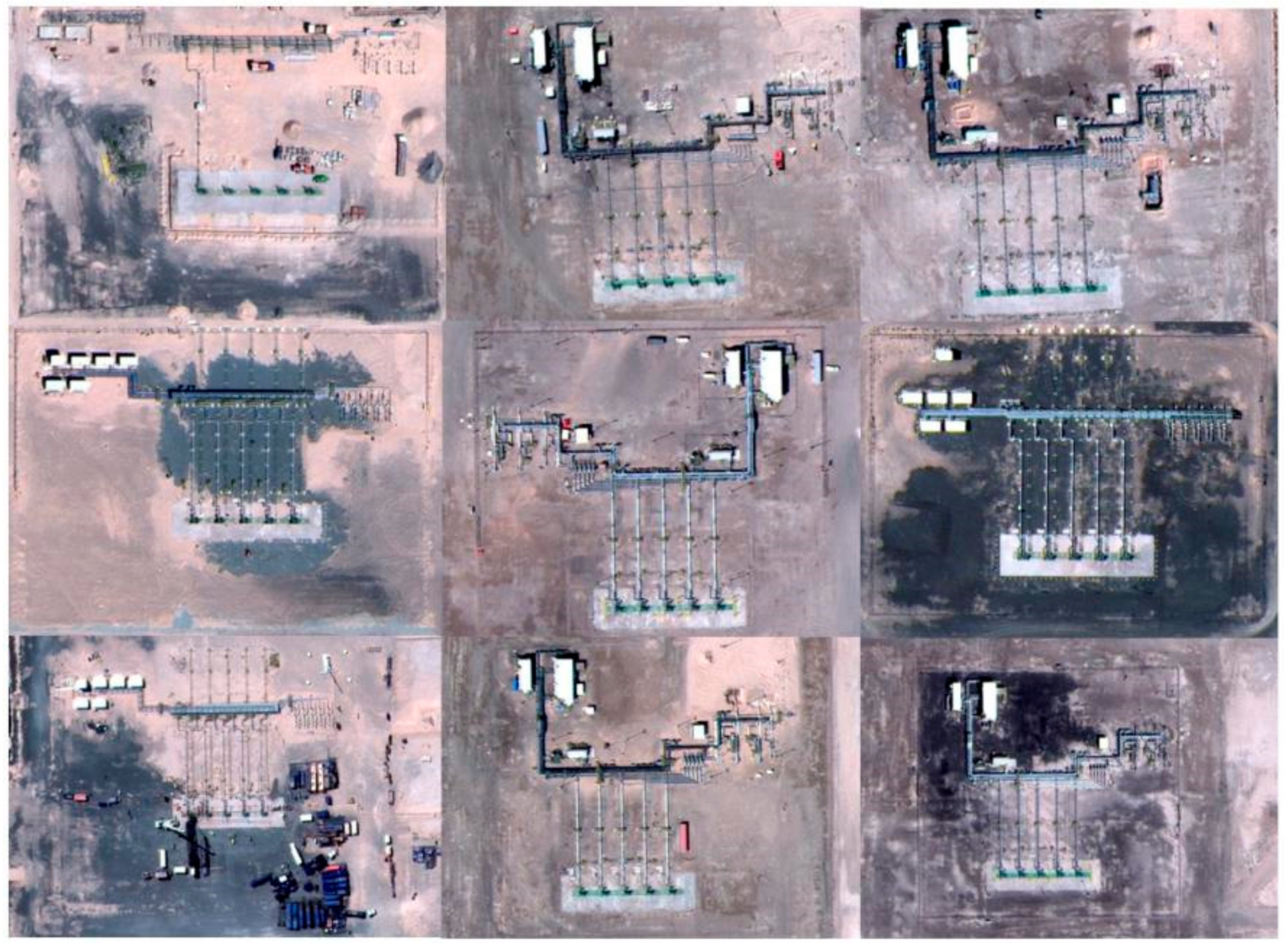
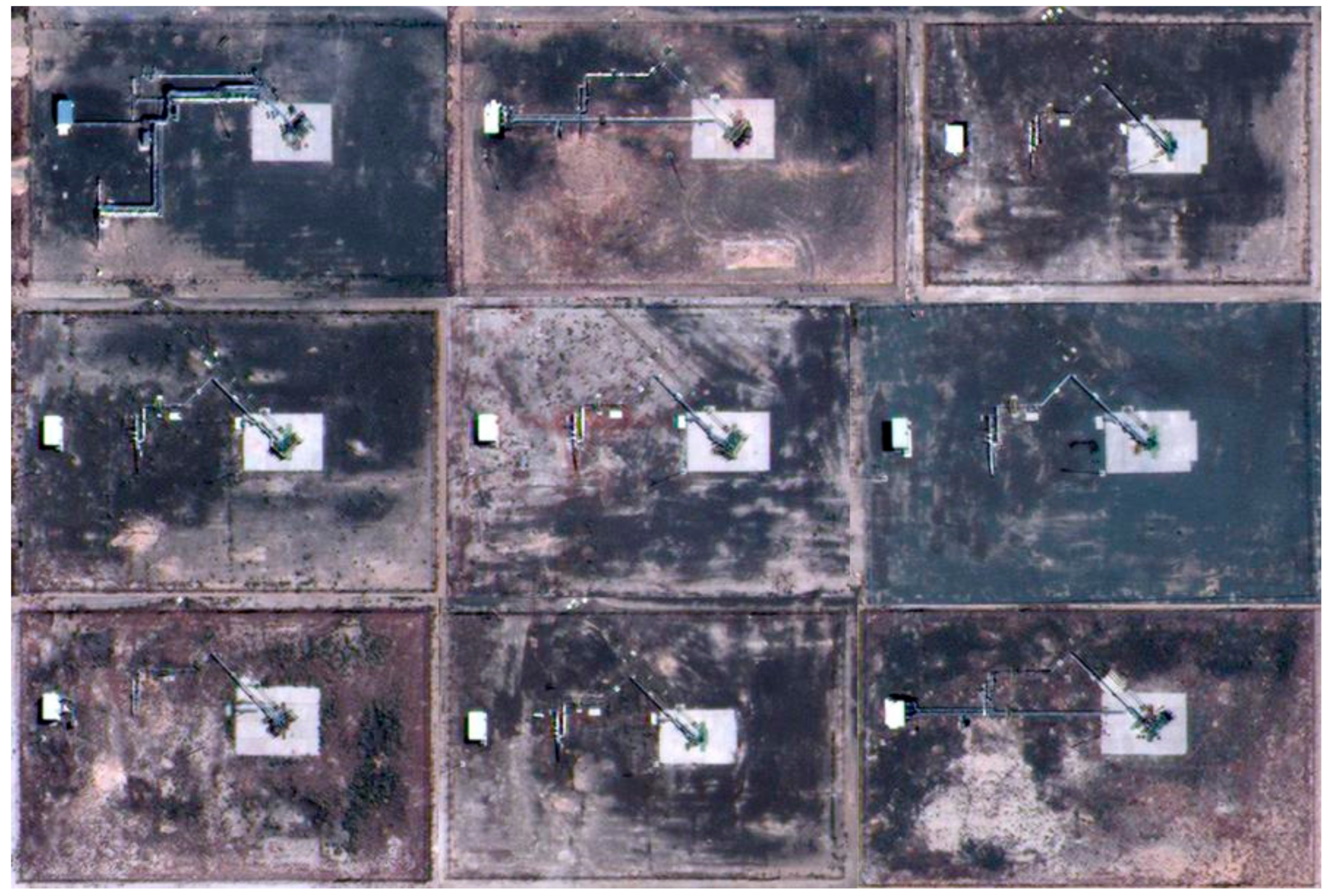
Figure 2.
Samples of well type 1 collected for the generation of image chips.
Figure 2.
Samples of well type 1 collected for the generation of image chips.
Figure 3.
Samples of well type 2 collected for the generation of image chips.
Figure 3.
Samples of well type 2 collected for the generation of image chips.
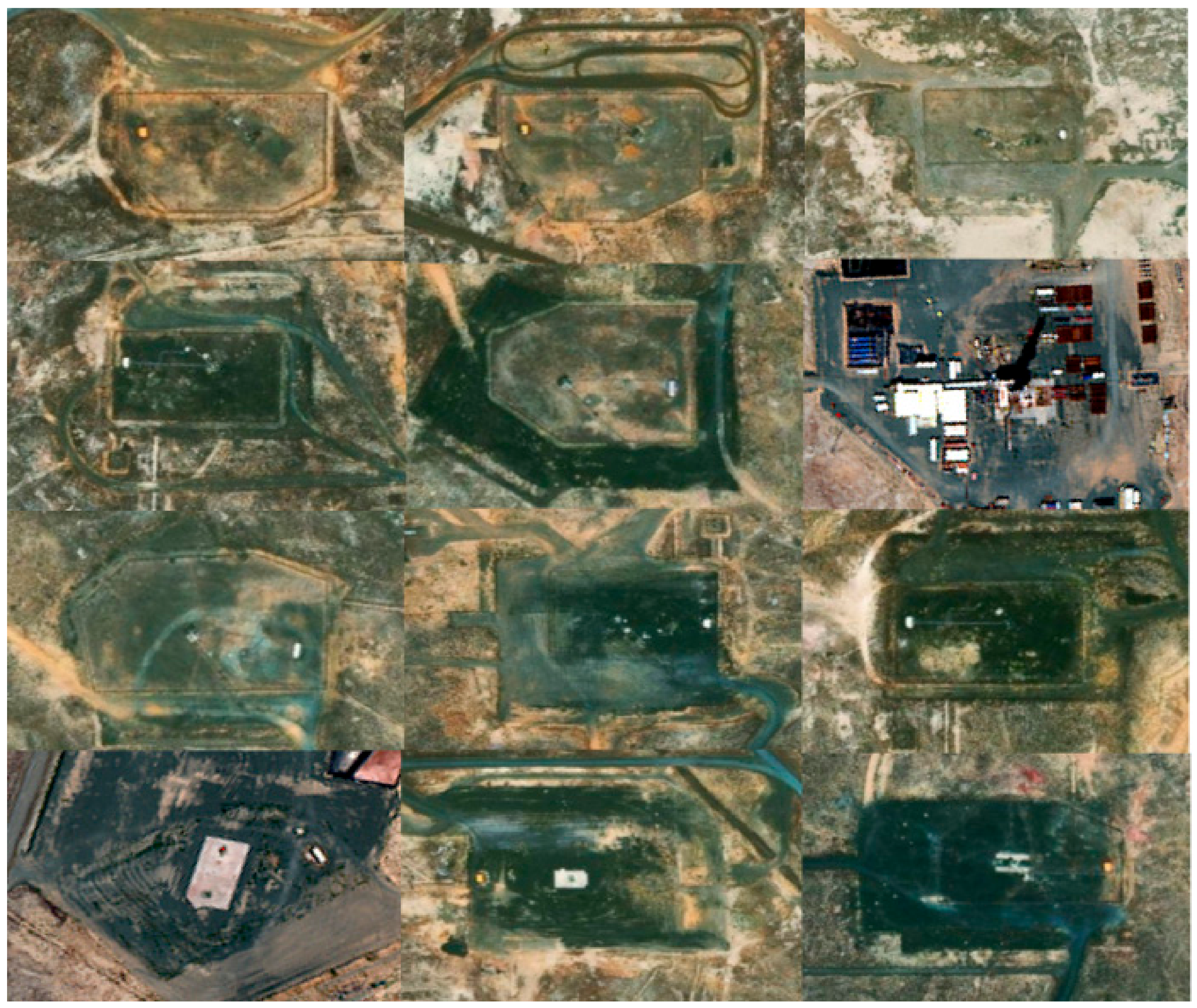
Figure 4.
Samples of well type 3 collected for the generation of image chips.
Figure 4.
Samples of well type 3 collected for the generation of image chips.
Figure 5.
Extents, acquisition periods, and counts of the TSX, CSK, and SNT1 images.
Figure 5.
Extents, acquisition periods, and counts of the TSX, CSK, and SNT1 images.
Figure 6.
Connection graphs: time–position and time–baseline plots for SBAS-InSAR: (a,b) CSK DSC; (c,d) CSK ASC right track; (e,f) CSK ASC left track; (g,h) TSX ASC; (i,j) SNT1 DSC; (k,l) SNT1 ASC.
Figure 6.
Connection graphs: time–position and time–baseline plots for SBAS-InSAR: (a,b) CSK DSC; (c,d) CSK ASC right track; (e,f) CSK ASC left track; (g,h) TSX ASC; (i,j) SNT1 DSC; (k,l) SNT1 ASC.
Figure 7.
Integrated workflow for the deep learning-based recognition of wellpads and SBAS-InSAR interferometric processing.
Figure 7.
Integrated workflow for the deep learning-based recognition of wellpads and SBAS-InSAR interferometric processing.
Figure 8.
Training and validation losses over epochs obtained by training a Mask R-CNN model based on 1.24 m resolution RGB images.
Figure 8.
Training and validation losses over epochs obtained by training a Mask R-CNN model based on 1.24 m resolution RGB images.
Figure 9.
Training and validation losses over epochs obtained by training a Mask R-CNN model based on pansharpened 0.3 m resolution RGB images.
Figure 9.
Training and validation losses over epochs obtained by training a Mask R-CNN model based on pansharpened 0.3 m resolution RGB images.
Figure 10.
Training polygons overlaid with detected polygons of wells.
Figure 10.
Training polygons overlaid with detected polygons of wells.
Figure 11.
Quantification of wellpads by (a) vertical displacement (VD) and (b) cumulative displacement (CD) classes.
Figure 11.
Quantification of wellpads by (a) vertical displacement (VD) and (b) cumulative displacement (CD) classes.
Figure 12.
(a) VD from SNT1; (b) CD from SNT1.
Figure 12.
(a) VD from SNT1; (b) CD from SNT1.
Figure 13.
(a) VD from CSK; (b) CD from CSK.
Figure 13.
(a) VD from CSK; (b) CD from CSK.
Figure 14.
(a) VD from TSX/CSK; (b) CD from TSX/CSK.
Figure 14.
(a) VD from TSX/CSK; (b) CD from TSX/CSK.
Figure 15.
Regression analysis for the (a) VD and (b) CD of wellpads.
Figure 15.
Regression analysis for the (a) VD and (b) CD of wellpads.
Figure 16.
CD for wellpads: (a) CSK—16 December 2020; (b) TSX/CSK—10 December 2020; (c) SNT1—24 December 2020; (d) SNT1—19 December 2021.
Figure 16.
CD for wellpads: (a) CSK—16 December 2020; (b) TSX/CSK—10 December 2020; (c) SNT1—24 December 2020; (d) SNT1—19 December 2021.
Figure 17.
Cumulative displacement predicted for 31 December 2023: (a) SNT1; (b) CSK; (c) TSX/CSK.
Figure 17.
Cumulative displacement predicted for 31 December 2023: (a) SNT1; (b) CSK; (c) TSX/CSK.
Figure 18.
Number of wells within cumulative displacements predicted for 31 December 2023.
Figure 18.
Number of wells within cumulative displacements predicted for 31 December 2023.
Figure 19.
(
a) Hydrological water flow; (
b) 3D model of vertical displacement velocity and reservoir depths (adapted from Bayramov et al. [
15]).
Figure 19.
(
a) Hydrological water flow; (
b) 3D model of vertical displacement velocity and reservoir depths (adapted from Bayramov et al. [
15]).
Table 1.
Characteristics of the Worldview-3 satellite image used for the present study (Satellite Imaging Corporation 2023, Tomball, TX, USA).
Table 1.
Characteristics of the Worldview-3 satellite image used for the present study (Satellite Imaging Corporation 2023, Tomball, TX, USA).
| Sensor Imaging Mode | Sensor Bands | Sensor Resolution (GSD) | Revisit Time (Days) | Dynamic Range | Swath Width |
|---|
| Worldview-3 | Panchromatic: 450-800 nm
8 Multispectral: (red, red edge, coastal, blue, green, yellow, near-IR1, and near-IR2) -400-1040 nm
8 SWIR: 1195-2365 nm | Panchromatic Nadir: 30 cm GSD at Nadir 0.34 m at 20° Off-Nadir
Multispectral Nadir: 1.24 m at Nadir, 1.38 m at 20° Off-Nadir
SWIR Nadir: 3.70 m at Nadir, 4.10 m at 20° Off-Nadir | 1 day at 1 m GSD resolution 4.5 days at 20° off-nadir (0.59 m GSD) | 11 bits per pixel Pan and MS; 14 bits per pixel SWIR | At nadir: 13.1 km |
Table 2.
Parameters for the preparation of training data, the training of the deep learning model, and object detection [
30,
31].
Table 2.
Parameters for the preparation of training data, the training of the deep learning model, and object detection [
30,
31].
| Input for Export Training Data for Deep Learning | Parameters | Description |
|---|
| Input Raster | TIFF (8 bit) | The input source imagery. |
| Tile Size X | 256 | The size of the image chips for the x dimension. |
| Tile Size Y | 256 | The size of the image chips for the y dimension. |
| Stride X | 128 | The distance to move in the x direction when creating the next image chips. |
| Stride Y | 128 | The distance to move in the y direction when creating the next image chips. |
| Reference System | Map Space | Type of reference system that will be used to interpret the input image. |
| Metadata Format | RCNN Masks | Format that will be used for the output metadata labels. |
| Input for Training the Deep Learning Model | | |
| Input Training Data | TIFF (8 bit) | The image chips, labels, and statistics required to train the model. |
| Max Epochs | 20 | The maximum number of epochs for which the model will be trained. |
| Model Type | Mask RCNN (Object detection) | The model type that will be used to train the deep learning model. |
| Batch Size | 4 | The number of training samples to be processed for training at one time. |
| Chip Size | 224 | The size of the images used to train the model. Images are cropped to the specified chip size. |
| Monitor | Valid loss | Specified metrics to monitor while checkpointing and early stopping. |
| Backbone Model | ResNet-50 | The specified preconfigured neural network to be used as the architecture for training the new model. |
| Validation (%) | 10 | The percentage of training samples that will be used for validating the model. |
| Input for Detecting Objects Using Deep Learning | | |
| Imagery Format | TIFF (8 bit) | The input source imagery. |
| Model Definition | Trained Model (dlpk) | This parameter can be an Esri model definition JSON file (.emd), a JSON string, or a deep learning model package (.dlpk). |
| Padding | 56 | The number of pixels at the border of image tiles from which predictions are blended for adjacent tiles. |
| Batch size | 4 | Number of image tiles the GPU can process at once while inferencing. |
| Threshold | 0.9 | Minimum level of confidence that will be included in the output. |
| Return boxes | False | Return bounding box is a Boolean parameter with a true or false input. |
| Tile size | 224 | The width and height of the image tiles into which the imagery is split for prediction. |
| Non-Maximum Suppression | Checked | Non-maximum suppression is performed, in which duplicate objects are identified and the duplicate features with lower confidence value are removed. |
Table 3.
Accuracy computation metrics for object detection [
32].
Table 3.
Accuracy computation metrics for object detection [
32].
| Accuracy Metrics | Description |
|---|
| Precision | The ratio of the number of true positives to the total number of positive predictions. |
| Recall | The ratio of the number of true positives to the total number of actual (relevant) objects. |
| F1_Score | The weighted average of the precision and recall. Values range from 0 to 1, where 1 is the highest accuracy. |
| The Average Precision (AP) metric | The Average Precision (AP) metric, which is the precision averaged across all recall values. |
| True_Positive | The number of true positives generated by the model. |
| False_Positive | The number of false positives generated by the model. |
| False_Negative | The number of false negatives generated by the model. |
Table 4.
Characteristics of the SAR images used for the present study [
36,
37].
Table 4.
Characteristics of the SAR images used for the present study [
36,
37].
| Sensor Imaging Mode | Track | Resolutions: Range x Azimuth [m × m] & Swath [km] | Revisit Time (Days) | Count of Images | Temporal Span | Polarization Used | Interferometric Mode | Wavelength |
|---|
| TerraSAR-X (TSX) | ACS | 3 × 3; 30 | 11 | 119 | 1 January 2018 and 31 December 2021 | HH | StripMap | X-band (3 cm, 9.65 GHz) |
COSMO-SkyMed (CSK)
Stripmap mode | DSC | 3 × 3; 40 | 4 | 87 | 1 January 2018 and 31 December 2020 | HH | StripMap HIMAGE | X-band
(3.1 cm, 9.6 GHz) |
| ASC | 28 |
| 60 |
| Sentinel-1 (SNT1) | DSC | 5 × 20; 250 | 6 | 117 | 1 January 2018 and 31 December 2021 | VV | Interferometric Wide Swath (IW) mode | C-band (5.6 cm wavelength and 5.4 GHz) |
| ASC | 121 |
| 114 |
Table 5.
Computed accuracy metrics for detected objects.
Table 5.
Computed accuracy metrics for detected objects.
| Precision | Recall | F1_Score | AP | True Positive | False Positive | False Negative |
|---|
| 0.713004 | 0.913793 | 0.801008 | 0.767871 | 159 | 64 | 15 |
Table 6.
Quantification of wellpads by VD and CD classes.
Table 6.
Quantification of wellpads by VD and CD classes.
| Count of Wells |
|---|
| Range of VD | SNT1 | CSK | TSX/CSK |
| −54–−40 | 13 | 8 | 20 |
| −39–−30 | 23 | 34 | 28 |
| −29–−20 | 28 | 39 | 35 |
| −19–−10 | 39 | 45 | 40 |
| −9–10 | 65 | 47 | 50 |
| 11–20 | 5 | 1 | 1 |
| 21–27 | 1 | | |
| TOTAL | 174 | 174 | 174 |
| Range of CD | SNT1 | CSK | TSX/CSK |
| −160–−140 | 3 | 1 | 5 |
| −139–−120 | 6 | 5 | 10 |
| −119–−100 | 15 | 19 | 20 |
| −99–−80 | 19 | 20 | 17 |
| −79–−60 | 16 | 26 | 25 |
| −59–−40 | 28 | 35 | 32 |
| −39–−20 | 32 | 31 | 22 |
| −19–0 | 23 | 24 | 28 |
| 1–20 | 15 | 9 | 12 |
| 21–40 | 14 | 3 | 2 |
| 41–60 | 2 | 1 | 1 |
| 61–80 | 1 | | |
| Total count | 174 | 174 | 174 |
Table 7.
Quantification of wellpads within predicted CD classes.
Table 7.
Quantification of wellpads within predicted CD classes.
| Number of Wells |
|---|
| Range of Predicted CD | SNT1 | CSK | TSX/CSK |
|---|
| −339–−320 | 0 | 0 | 2 |
| −319–−300 | 1 | 0 | 2 |
| −299–−280 | 2 | 4 | 1 |
| −279–−260 | 2 | 2 | 6 |
| −259–−240 | 5 | 2 | 4 |
| −239–−220 | 7 | 11 | 14 |
| −219–−200 | 7 | 13 | 7 |
| −199–−180 | 8 | 10 | 9 |
| −179–−160 | 10 | 10 | 10 |
| −159–−140 | 9 | 10 | 12 |
| −139–−120 | 7 | 18 | 11 |
| −119–−100 | 13 | 12 | 16 |
| −99–−80 | 16 | 19 | 17 |
| −79–−60 | 15 | 14 | 12 |
| −59–−40 | 16 | 14 | 8 |
| −39–−20 | 7 | 10 | 14 |
| −19–0 | 19 | 12 | 12 |
| 1–20 | 4 | 6 | 8 |
| 21–40 | 8 | 3 | 5 |
| 41–60 | 12 | 3 | 3 |
| 61–80 | 3 | 0 | 0 |
| 81–100 | 2 | 0 | 0 |
| 101–120 | 0 | 1 | 1 |
| 141–150 | 1 | 0 | 0 |
| Total count | 174 | 174 | 174 |
| Disclaimer/Publisher’s Note: The statements, opinions and data contained in all publications are solely those of the individual author(s) and contributor(s) and not of MDPI and/or the editor(s). MDPI and/or the editor(s) disclaim responsibility for any injury to people or property resulting from any ideas, methods, instructions or products referred to in the content. |
© 2024 by the authors. Licensee MDPI, Basel, Switzerland. This article is an open access article distributed under the terms and conditions of the Creative Commons Attribution (CC BY) license (https://creativecommons.org/licenses/by/4.0/).


