Development and Calibration of 532 nm Standard Aerosol Lidar with Low Blind Area

Abstract

To better calibrate the aerosol lidar network constructed by the China Meteorological Administration, and ensure the data quality observed by the network, the Meteorological Observation Center (China Meteorological Administration) and the University of Naples (Italy) jointly developed a “high quality 532 nm Raman aerosol lidar” (REAL lidar) in 2018. The ability to detect Raman–Mie scattering signals was improved through signal detection in a large dynamic range. This study compared the REAL lidar with the reference lidar (European ACTRIS aerosol lidar network) considering three wavelengths and eight channels. The results show that both the original signals and data products of the two radars exhibited good consistency. In the calibration application of China’s domestic lidar network, after REAL calibration, the relative average and standard deviations of the backscattering coefficient of the in-station lidar decreased from 55.4% to 7.9% and from 64% to 9.9%, respectively. The effect was significant, which indicates that REAL is an aerosol lidar with a high-performance index. The results satisfy the demand for calibration of the aerosol lidar network, and the REAL was successfully applied to the calibration of the aerosol lidar network.

1. Introduction

Lidar calibration has always plagued the processing of lidar data and unification of observation data. Lidar calibration and rendering lidar detection data quantitatively comparable are common problems encountered by all. The ACTRIS aerosol lidar network in Europe (originally the EARLINET Aerosol lidar network) is among the aerosol lidar networks that exhibit good performance. The standard calibration methods include centralized contrast calibration and the use of standard aerosol lidar for station calibration [1,2,3].

ACTRIS lidar network calibration has been performed regularly since the end of the 1990s, and comparative aerosol lidar calibration in the network is conducted annually [4,5,6]. During 2009–2013, the deviation of the echo signal of all channels of the 21 lidars in the lidar network was less than ±2% within a specific altitude range. In addition, the variation ranges of the calculated aerosol backscattering and extinction coefficients were less than 2 × 10⁻⁴ km⁻¹sr⁻¹ and 0.01 km⁻¹, respectively. The high-precision data products detected by the lidars in the network are vital to the numerical models and ground calibration of spaceborne lidars in Europe and America. The ash distribution and concentration products detected by the network can provide aviation meteorological services for aircraft and improve the service life of aircraft engines [7,8].

The multiwavelength system for aerosol (MUSA) is a referential lidar system in the ACTRIS framework. The lidar instrument is equipped with three elastic channels working at 355, 532, and 1064 nm, and two inelastic N₂ Raman channels at 387 and 607 nm. Two independent polarization components of the elastic channel at 532 nm are used to measure the particle depolarizability. Further, all channels are collected in analog and photon counting modes to improve the detectable dynamic range [9]. The calibration of near-surface data is important for standard lidars based on the detection requirements of the low boundary layer range; however, the MUSA standard lidar has an overlap range of approximately 250–300 m, and there are still certain limitations in the near-surface data corrections of lidars with no or low blind areas.

Many universities and research institutes have undertaken the development of aerosol lidars in China [10,11,12,13,14,15]. With the frequent occurrence of urban haze weather, aerosol lidars have been gradually added to the equipment of meteorological and environmental protection departments [16]. Therefore, it is necessary for us to develop a standard lidar with low blind area and high dynamic gain for the calibration of China’s lidar network.

With the help of the University of Naples, the Meteorological Detection Center of China Meteorological Administration developed a high-quality 532 nm Raman–Mie aerosol lidar (REAL) that is used as the standard lidar for the calibration of other aerosol lidars. The lidar was compared with the standard lidar of the ACTRIS lidar network in Europe, and the original signal, depolarization ratio product, and extinction coefficient measured by the lidar were found to have reached the required level for weather service application. In order to ensure that the REAL reached the calibration requirements of the ACTRIS aerosol lidar network, a comparison to the MUSA as the reference lidar was conducted in Potenza, Italy. A comparative analysis was conducted on the original data, 532 nm depolarization ratio, and backscattering coefficient, and the results showed a good consistency and the REAL reached the calibration requirement of the MUSA. The REAL was also used effectively in a series of field campaigns in China.

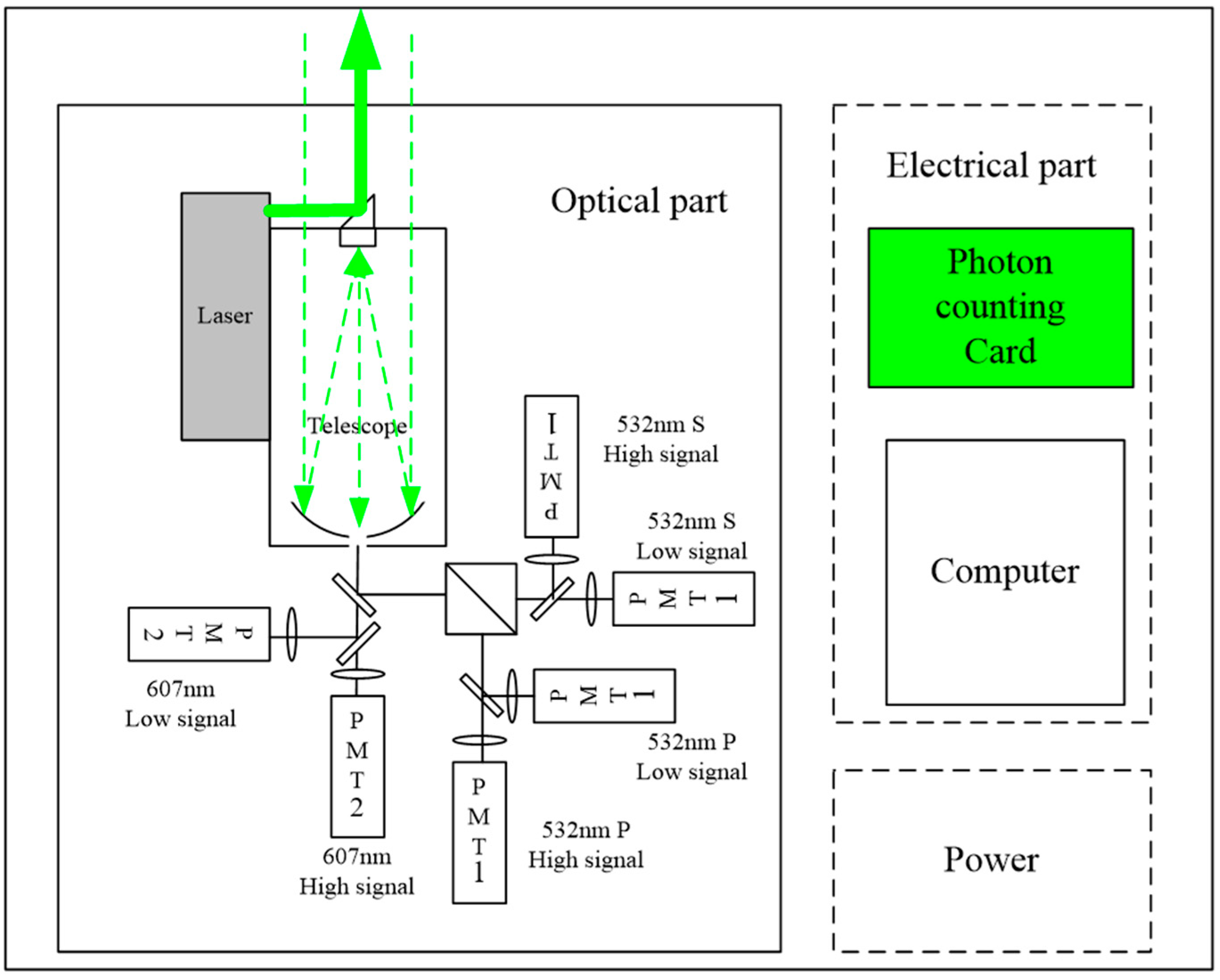
2. REAL with Low Bow Blind Area and High Dynamic Gain

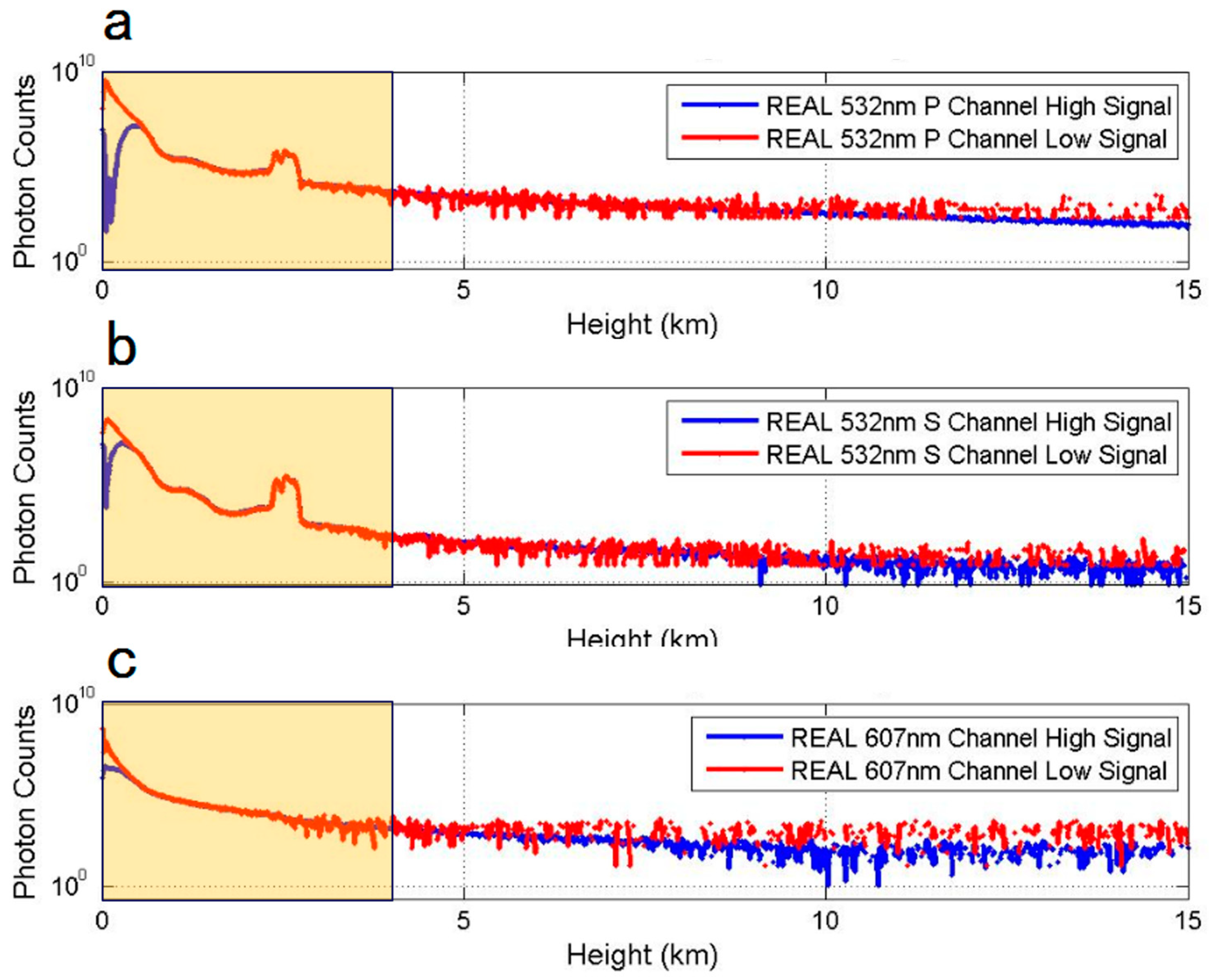
2.1. Six-Channel Raman–Mie Scattering Detection

REAL is a single-wavelength Raman–Mie scattering aerosol LiDAR with the emission wavelength of 532 nm. The receiver is divided into six channels, among which the primary receiver channels are a 532 nm parallel polarization channel (532 nm P), 532 nm perpendicular polarization channel (532 nm S), and 607 nm N₂ Raman channel (607 nm). Figure 1 shows the system schematic of the lidar. The four PMT1s in the figure are the same type of detectors, mainly used for the detection of elastic signals. PMT2s are the same type of high-performance detectors (cooling), mainly used for the detection of Raman signals. In general, the dynamic range of the available detectors is smaller than that of the lidar signal. To ensure the dynamic range of the data from the three main receiving channels, each main receiving channel is divided into high and low channels by an unpolarization beamsplitter and uses a different attenuator. All the high channels are used to detect signals from a high altitude, the attenuation coefficients of the attenuators in these channels are set at a low value, and the signal–noise ratio (SNR) of the high-altitude signals is high. Thus, a large detection range is achieved; however, the low-altitude signals are saturated. In addition, the attenuation coefficients in low channels are set at a high value to prevent the saturation of low-altitude signals and obtain the maximum effective detection signal. To improve the dynamic range of the lidar echo signal, the two sub-channels realize data fusion using linear overlap. The main parameters of the REAL are listed in

Table 1. Main parameters of the 532 nm Raman–Mie aerosol lidar.

Parameters	Specification
Laser system
Wavelength	532 nm
Repetition frequency	1000 Hz
Average power	≥2 W
Cooling method	Air-cooled
Receiving system
Telescope diameter	250 mm
Photoelectric converter	PMT
Interference filter	≤1 nm
Receiving channel	532 nm P channel high signal 532 nm P channel low signal 532 nm S channel high signal 532 nm S channel low signal 607 nm channel high signal 607 nm channel low signal
Data acquisition boards	Photon counter

.

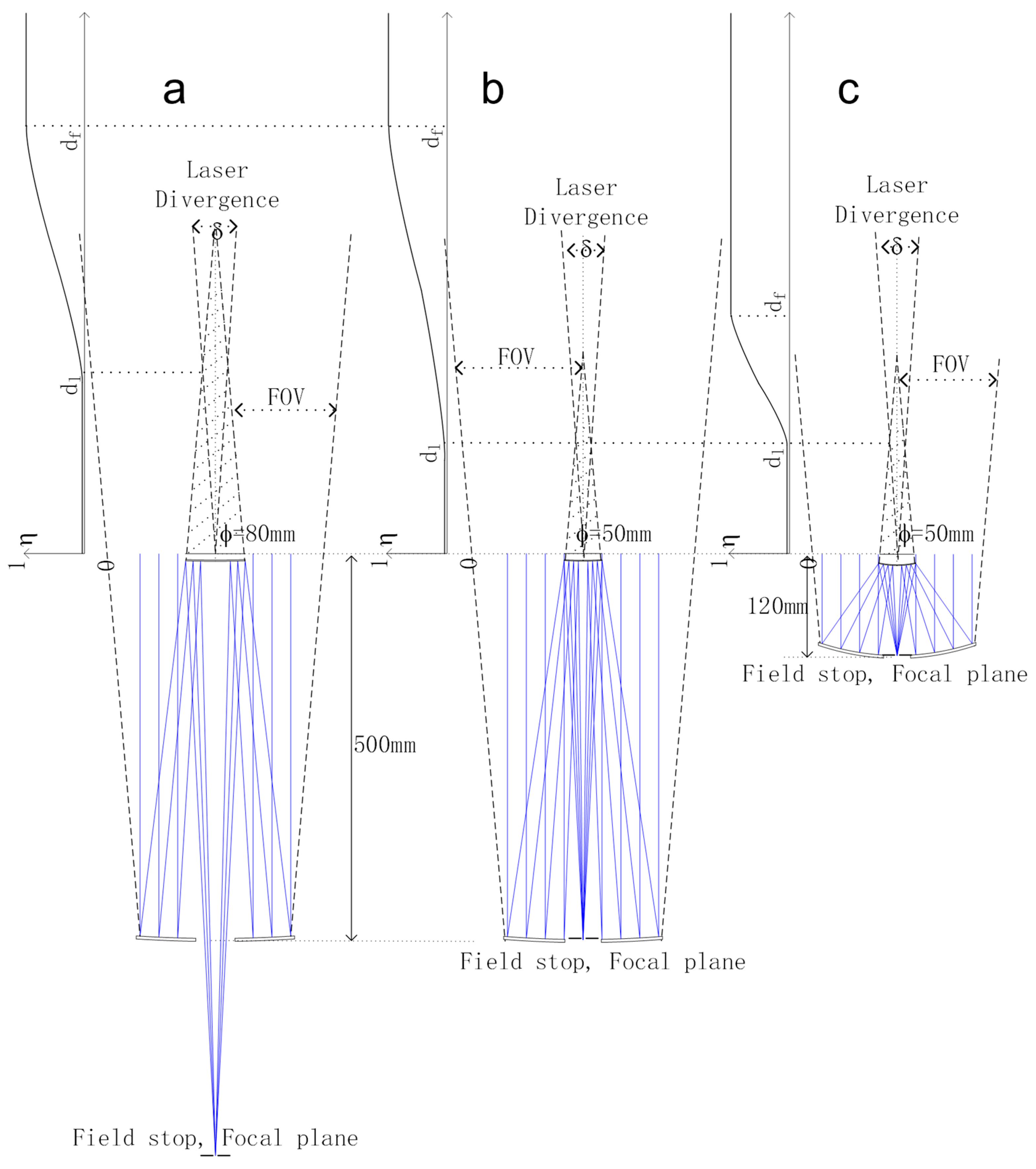
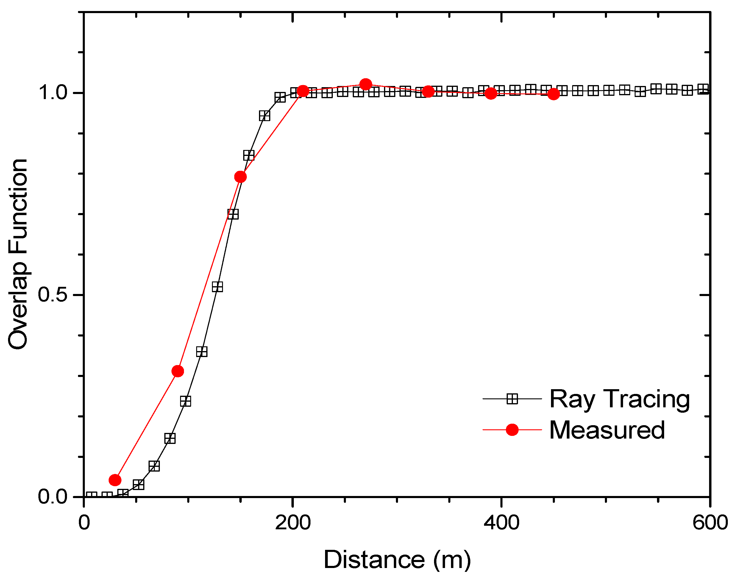
2.2. Low Blind Zone Optical Design

The aerosol lidar mostly adopts a coaxial optical system design, which is capable of detecting blind and overlap areas and limiting the lidar echo at low altitudes. Considering the design of the receiving system, reducing the range of the blind and overlap areas of the lidar system is key to improving the low-altitude detection ability of aerosol lidar.

The optical efficiency of lidar in the near field is primarily determined by the overlap function η. Figure 2 shows an example of the telescope structure design. The overlap function η can be divided into three parts as per different areas: the blind area (0 < $d$ < $d_l$, η = 0), incomplete overlap area ($d_l$ < $d$ < $d_f$, 0 < η), and complete overlap area ($d_f$ < $d$ < ∞, η = 1). The distance $d_l$ of the blind zone can be obtained from the geometric relationship in Figure 2:

$$d_l=\frac{\phi }{\delta +FOV}$$

(1)

where $\phi$ is the diameter of the secondary mirror of the telescope, $\delta$ is the divergence angle of the laser beam, and $FOV$ is the field of view of the telescope. In Figure 2, a is the diameter of the field diaphragm and $f$ is the focal length of the telescope. When $\delta$ and the $FOV$ are constant, the lidar blind zone $d_l$ is proportional to $\phi$.

At first, the focal plane of the telescope is set below the main mirror, and then the focal plane is moved to the position of the apex of the main mirror. As the distance between the focal plane and secondary mirror is reduced, the blind zone can be reduced effectively by reducing the diameter of the secondary mirror under the same telescope exit aperture angle. Moreover, the reduction of its diameter also decreases the shading area of the secondary mirror and increases the detection efficiency. For example, for the parameters of Φ = 200 mm, $f$ = 2000 mm, and F = 10, the distance between the primary mirror and the secondary mirror was 500 mm, $FOV$ = 1 mrad, and the laser divergence angle $\delta$ = 0.5 mrad. When the focal plane was moved up from 288 mm below the telescope to the apex of the primary mirror, the diameter of the secondary mirror was reduced from 80 mm (Figure 2a) to 50 mm (Figure 2b). Further, the shading area was reduced by 2.56 times, and the length of the blind zone $d_l$ was reduced from 53 to 33 m.

The minimized complete overlap distance $d_f$ is related to the telescope focal length f as the telescope’s F-number. From the lens formula $\raisebox{1ex}{$1$}\!\left/ \!\raisebox{-1ex}{$f$}\right.=1/u+\raisebox{1ex}{$1$}\!\left/ \!\raisebox{-1ex}{$v$}\right.$, the formula $u=\raisebox{1ex}{$fv$}\!\left/ \!\raisebox{-1ex}{$(v-f)$}\right.$ can be obtained, and then the following formula can be obtained:

$$u=\left[\frac{1}{\frac{v-f}{f}}+1\right]f$$

(2)

where $u$ is the object distance and $v$ is the image distance. The field diaphragm of the telescope is placed at the focal plane of the telescope, where $\raisebox{1ex}{$(v-f)$}\!\left/ \!\raisebox{-1ex}{$f$}\right.$ represents the relative deviation of the image distance $v$ of the laser spot, relative to the field diaphragm, when the object distance $u$ is finite.

When the image spot is at the position of the field diaphragm, this deviation is very small, the lidar system can receive the entire signal. This is the complete overlap region of the lidar. When $u$ is a finite distance, the laser spot is imaged below the field diaphragm, whereas if the distance $v$ is far from $f$, it results in a relatively large value of the deviation $\raisebox{1ex}{$(v-f)$}\!\left/ \!\raisebox{-1ex}{$f$}\right.$. The receiving system can only receive a part of the laser scattering energy, which indicates the incomplete overlap region of the lidar. Moreover, the minimum complete overlap distance $d_f$ is proportional to the focal length $f$ of the telescope.

As the $FOV$ of the telescope is larger than the divergence angle of the laser, generally, when $\raisebox{1ex}{$(v-f)$}\!\left/ \!\raisebox{-1ex}{$f$}\right.\le 0.5\%$, all scattered light can enter the field diaphragm without being blocked. Consequently, according to Formula (2), the minimum complete overlap distance $d_f=201f$. Therefore, reducing the F of the telescope reduces the geometric length of the telescope, and rapidly decreases the height of the minimum complete overlap zone of the lidar.

Figure 2c is a telescope structure with a small F, where the focal plane is set at the position of the apex of the main mirror. The parameters were F = 2.5, $f$ = 500 mm, primary lens diameter = 200 mm, and secondary lens diameter = 50 mm, and the distance between primary and secondary lenses was 120 mm. Through experiments, the blind area and overlap region of this lidar were measured to be less than 50 and 200 m, respectively. Thus, the optimal design of the low blind area receiving system greatly improved the ability of aerosol detection at low altitude.

2.3. Fusion of High and Low Space Signals and Optimization of Dynamic Range

The numerical span of lidar echo signal intensity is very large, and thus a single receiving channel may lead to saturation at low altitude and low SNR at high altitude. REAL uses high- and low-altitude signal acquisition channels to collect data simultaneously, and then fuses these signals to obtain the complete signal in the whole range. Because the signals of the high- and low-level channels are collected simultaneously, the structural characteristics of the signals of the high- and low-level channels are consistent, and there is an overlap region for the effective detection signals from both the high- and low-level channels. Consequently, the distance-squared correction signal is obtained by preprocessing the high- and low-altitude data and then dividing the low-altitude signal by the high-altitude signal to obtain the ratio profile. Subsequently, the screening threshold was set in the profile to find the overlap region with a stable ratio as the fusion region. The average value of the ratio within the interval was calculated, and the high- and low-altitude channel signals were normalized and combined to create a complete signal and thus improve the dynamic range of the whole echo signal.

Figure 3 is an example of the result of REAL high space fusion. The box interval is the fusion interval. After fusion, the signal dynamic range of lidar was improved by 1–2 orders of magnitude.

3. REAL Self-Test Data Analysis

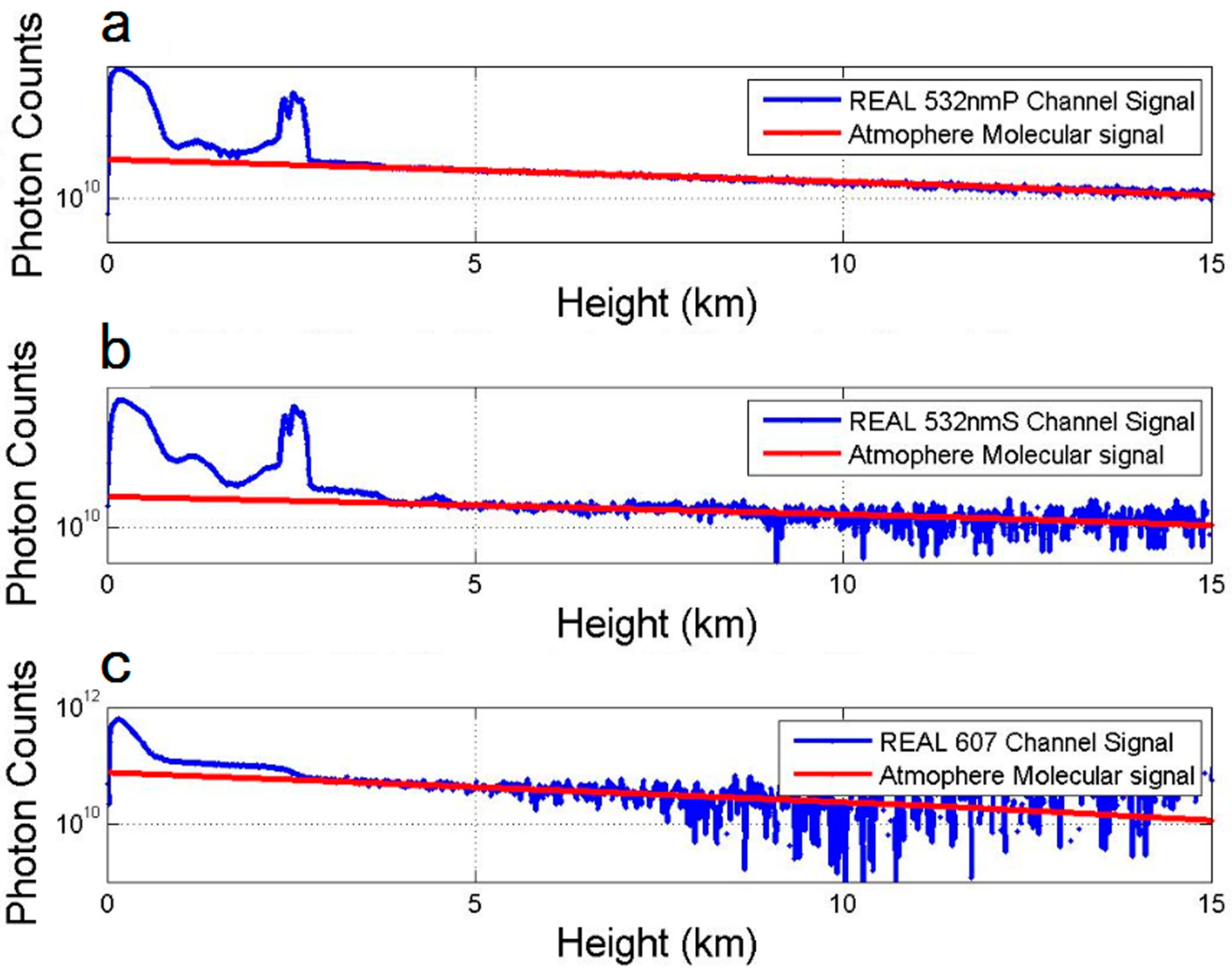
3.1. Consistency Analysis between REAL Echo Signal and Atmospheric Molecular Model Signal

To illustrate the accuracy of the REAL echo signal, the REAL 532 nm P, 532 nm S, and 607 nm channel echo signals were compared and analyzed with the atmospheric molecular echo signals calculated by the model. The 532 nm P channel of REAL in the range of 4–15 km height (Figure 4a), the 532 nm S channel in the range of 5–15 km height (Figure 4b), and the 607 nm channel in the range of 4–10 km height (Figure 4c) exhibited good consistency with the molecular echo signal.

For the height range of 5–10 km, the system difference and standard deviation of the three channels are presented in

Table 2. Comparison error of 532 nm P, 532 nm S, and 607 nm channels in 5–10 km range.

Channel	Relative Error		Relative Standard Deviation
	5–7 km	7–10 km	5–7 km	5–7 km
532 nm P	0.63%	3.6%	532 nm P	0.63%
532 nm S	−0.07%	−8.7%	532 nm S	−0.07%
607 nm	−1.7%	9.5%	607 nm	−1.7%

. The systematic errors for the 5–7 and 7–10 km ranges were less than 2% and 10%, respectively, which satisfy the design requirements. The relative standard deviations of the 532 nm S and 607 nm channels at 7–10 km were relatively larger, which was attributed to the reduction of the SNR of the detection signal.

3.2. REAL Low Blind Zone Data Analysis

According to the optical design requirements of the receiving system, Figure 5 shows the geometric factors obtained by the simulation of the optical path using the raytracing method of Zemax 13 optical design software in non-sequential mode [17]. Further, it was compared with the geometric factors calculated by the elastic scattering signals of the Raman signals in REAL [18]. The two were consistent. The range of the blind zone was less than 50 m and the full overlap distance was less than 200 m. Thus, compared with MUSA, REAL significantly improved the detection capability for low-altitude signals.

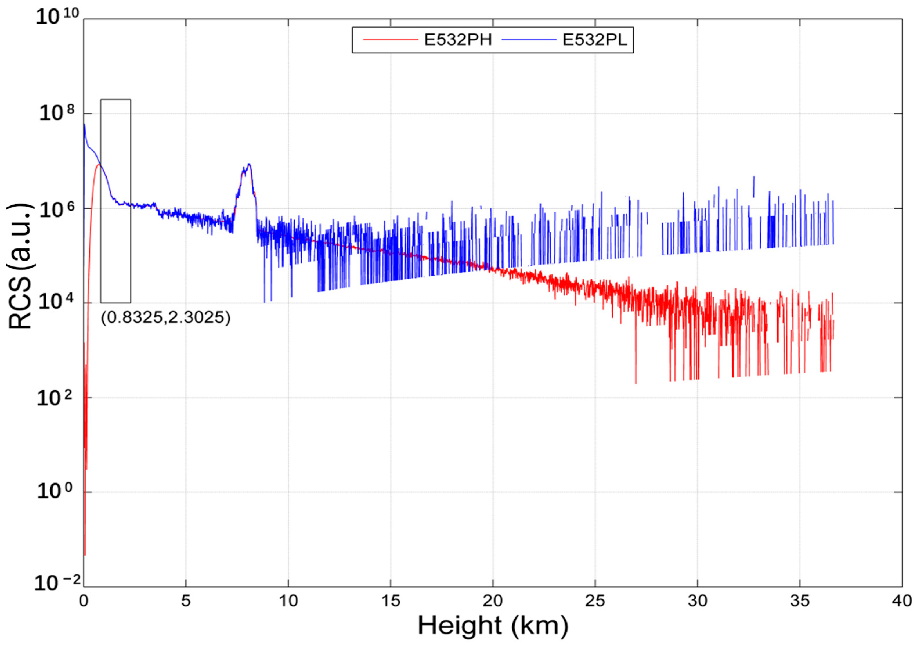
3.3. Dynamic Range Analysis of REAL Signal

REAL adopted high–low altitude separating signal acquisition systems for the 532 nm P, 532 nm S, and 607 nm channels. The high–low altitude echo signals of the three channels are shown in Figure 6. The high and low altitude signals of the 532 nm P, 532 nm S, and 607 nm channels were very consistent in the altitude range of 1–4 km. The ratio of the maximum value of the raw signal to the value of the raw signal where the signal-to-noise ratio is equal to 3 is the dynamic range.

Table 3. Table of dynamic range change after high and low space signal fitting of 532 nm P, 532 nm S, and 607 nm channels.

Channel	High Signal Channel Dynamic Range	The Change in Dynamic Range of the Signal after Fusing
532 nm P	3.3 × 109	≥200 times
532 nm S	2.2 × 108	≥10 times
607 nm	8.9 × 107	≥20 times

shows the change in dynamic range obtained by comparative analysis of REAL high–low space fusion signals. The fused signal dynamic ranges of 532 nm P, 532 nm S, and 607 nm were increased by at least 200, 10, and 20 times, respectively.

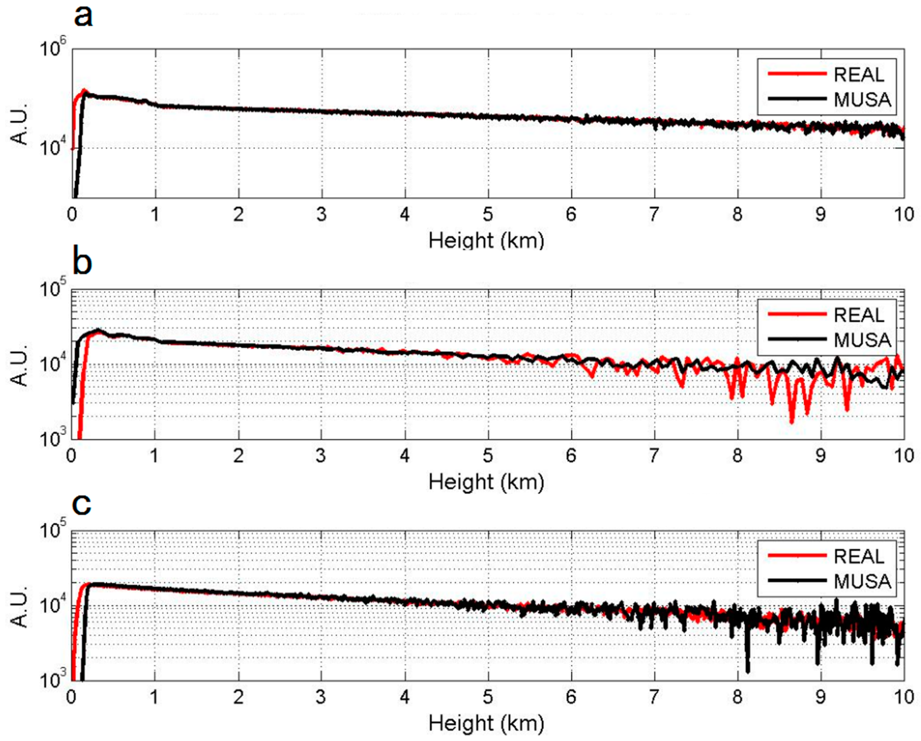
4. Comparative Analysis of REAL and MUSA Detection Data

4.1. Data Analysis Method

To compare the REAL and MUSA radar detection data, the relative average and standard deviations of the original signal were calculated and analyzed. In addition, the average and standard deviations of the polarization product were calculated and analyzed. The average deviation calculation and relative average deviation method were as follows:

$${\sigma }_{sys}=\frac{{\sum }_{k=1}^n(x_{1k}-x_{2k})}{n}$$

(3)

$$R_{sys}=\frac{{\sigma }_{sys}}{\overline{x_{2k}}}=\frac{\frac{{\sum }_{k=1}^n(x_{1k}-x_{2k})}{\overline{x_{2k}}}}{n}$$

(4)

The standard and relative standard deviations were calculated as follows:

$${\sigma }_{std}=(\frac{{\sum }_{k=1}^n(x_{1k}-x_{2k}{)}^2}{n}{)}^{1/2}$$

(5)

$$R_{std,i}=(\frac{{\sum }_{k=1}^n(x_{1k}-x_{2k}{)}^2}{n}{)}^{1/2}/\overline{x_{2k}}$$

(6)

where $x_{1k}$ and $x_{2k}$ are the measured signal values of REAL and MUSA at different range gates, and n is the calculated range gate value. The average deviation represents the systematic difference between the data profiles of REAL and MUSA, whereas the standard deviation represents the jitter of the data profiles of REAL relative to MUSA.

4.2. Comparative Analysis of Original Data

In Potenza, Italy, REAL and MUSA were calibrated on 12–13 November 2018. The calibration was conducted in two phases. The comparison of elastic scattering and Raman signals at night was conducted between 18:30 and 21:30 on 12 November, and the comparison of elastic scattering signals during the day was conducted between 12:00 and 15:00 on 13 November.

Figure 7 shows the comparison of the signals received by REAL and MUSA. The received signal from the 532 nm elastic P channel during the day and at night and that from the 607 nm Raman channel at night are illustrated.

It is evident from Figure 7 that the original signals of the 532 nm P and 607 nm channels of the REAL and MUSA lidars were consistent. Meanwhile, the low-altitude blind area of REAL was significantly smaller than that of MUSA, and the dynamic range was higher than that of MUSA. Further, a statistical analysis was conducted on the signals within the range of 0.5-5 km of the three channels, as shown in

Table 4. Comparison and analysis of original 532 nm P channel signals between REAL and MUSA.

Channel with Resolution	Results
	0.5–2 km		2–4 km		4–5 km
	Relative Mean Deviation	Relative Standard Deviation	Relative Mean Deviation	Relative Standard Deviation	Relative Mean Deviation	Relative Standard Deviation
532 nm P (15 m, nighttime)	−2.1%	3.2%	0.2%	3.2%	−0.4%	4.7%
532 nm P (60 m, daytime)	−0.0%	2.0%	−2.3%	7.8%	−1.5%	13.3%
607 nm (15 m)	−2.1%	2.5%	1.1%	4.3%	0.5%	7.6%

. It is evident that for the 532 nm P signal detected at night (Figure 7a) in the range below 2 km, the relative average and standard deviations were less than 2.1% and 3.2%, respectively; for the 532 nm P signal detected during the day (Figure 7b), the relative mean and standard deviations were less than 0.1% and 2.0%, respectively; and for the 607 nm channel signal (Figure 7c), the relative mean and standard deviations were less than 2.1% and 2.5%, respectively. In the ranges of 2–4 and 4–5 km, the relative average and standard deviations of each wavelength were less than 2% and 15%, respectively. The higher error was attributed to the decrease in SNR.

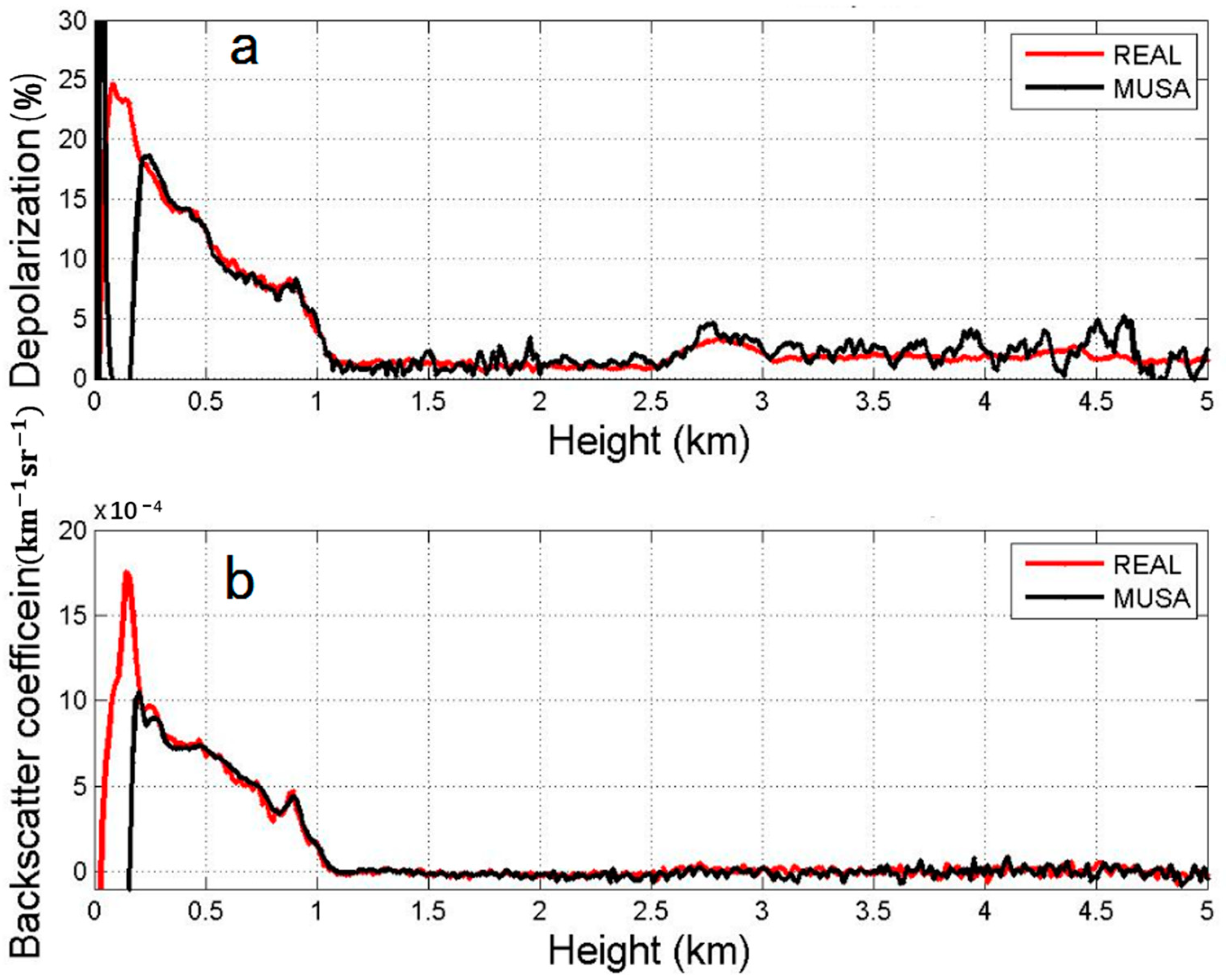
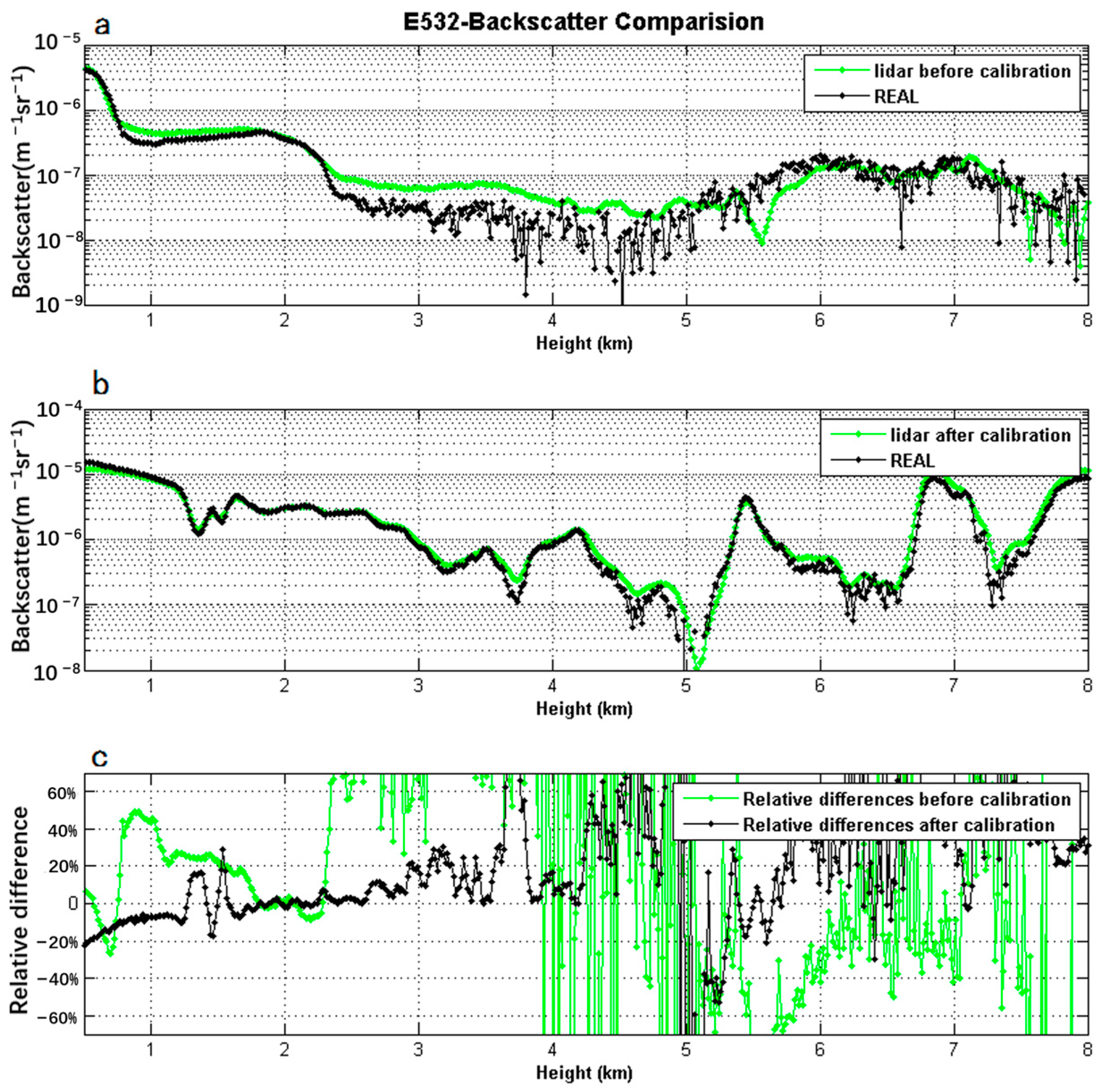
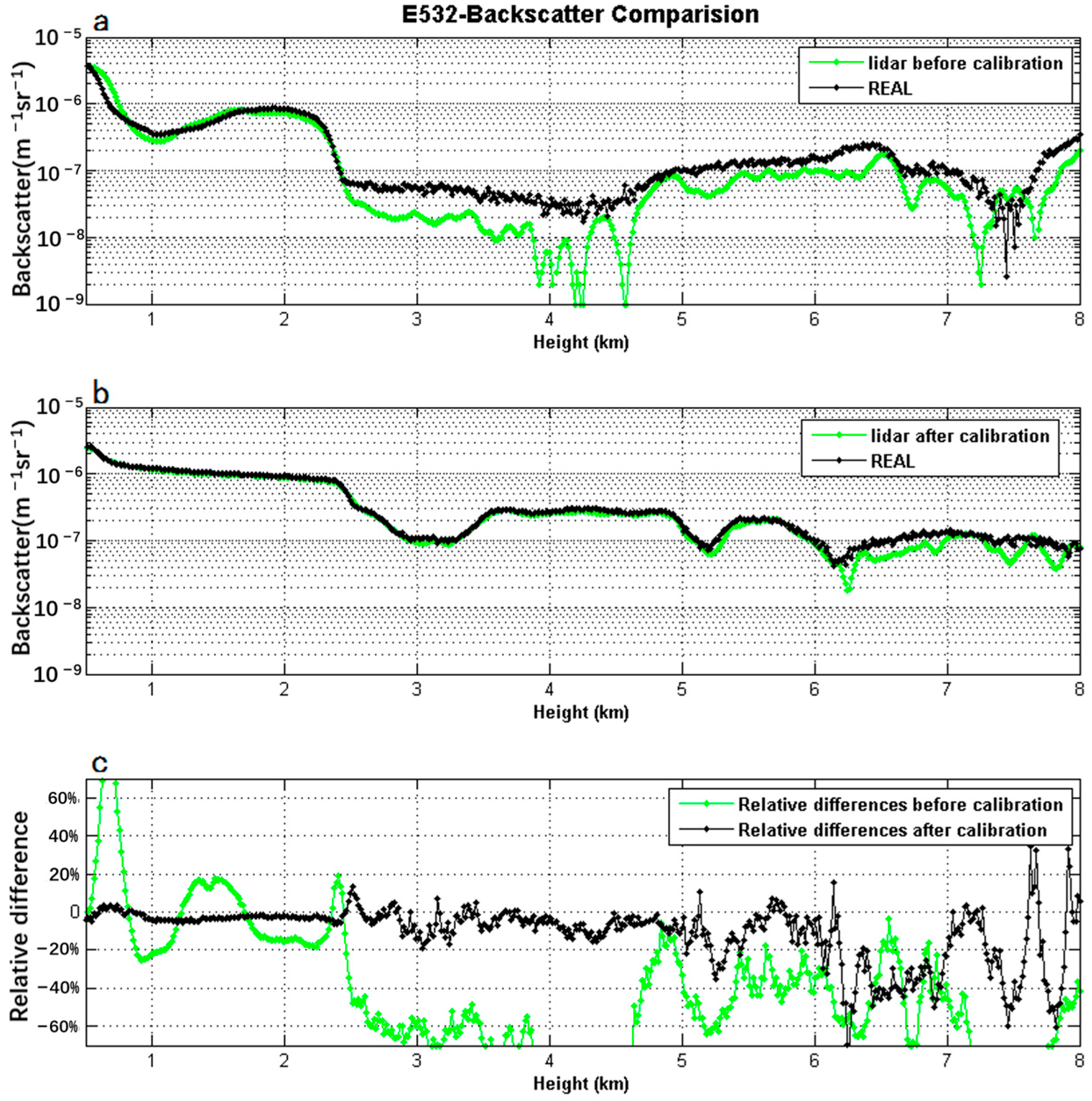
5. Comparative Analysis of 532 nm Depolarization Ratio and Backscattering Coefficient Products

The 532 nm P and 532 nm S channel signals of REAL and MUSA from 19:00 to 19:30 on 12 November 2018 were selected to calculate the depolarization ratio and backscattering coefficient products, as shown in Figure 8. The 15 m range resolution was used to compare the product data between 0.3 and 3 km, and the results are presented in

Table 5. Comparative analysis of depolarization ratio and backscatter coefficient of 532 nm channel between REAL and MUSA.

	Depolarization				Backscatter Coefficient
	Mean Deviation (%)	Relative Deviation (%)	Standard Deviation (%)	Relative Standard Deviation (%)	Mean Deviation (sr−1m−1)	Relative Deviation (%)	Standard Deviation (sr−1m−1)	Relative Standard Deviation (%)
0.3–1 km	−0.017	−0.189	0.059	0.656	1.1 × 10−8	1.556	3.6 × 10−8	5.143
1–2 km	−0.049%	\	0.60%	\	2.7 × 10−9	\	1.3 × 10−8	\
2–3 km	0.20%	\	0.30%	\	−1.1 × 10−8	\	2.4 × 10−8	\

. In the range of 0.3–3 km height, the average and standard deviations of the depolarization ratio were less than 0.05% and 0.60%, respectively. Further, the average and standard deviations of the backscatter coefficient were less than 1.1 × 10⁻⁸ and 3.6 × 10⁻⁸, respectively, which satisfy the European calibration standard.

6. Application Research of REAL

Following the alignment calibration with ACTRIS in Italy, REAL can be considered as the standard source of dissemination of quantity value. To ensure the measured results of the China’s aerosol lidar network were quantitatively comparable, REAL was added to a series of field campaigns for aerosol lidar calibration in Beijing, Shanghai, Guangzhou, and other big cities.

It was used to analyze the consistency of atmospheric echo signals and improve the detection accuracy of lidar at different stations. Figure 9 shows the comparison results of the aerosol backscatter coefficients before and after calibration. Within the range of 2–5 km, the average and standard deviations of the lidar backscatter coefficients at the station decreased from 55.4% to 7.9% and from 64.0% to 9.9%, respectively. Another similar result is shown in Figure 10 for another tested lidar. Thus, through comparative data statistics, it was confirmed that the detection accuracy of the lidar network can be effectively improved by using REAL, and the relative standard deviation of the aerosol backscatter coefficient was less than 20% (1–2 km) and 40% (2–5 km) [19,20].

7. Conclusions

Lidar calibration and rendering lidar detection data quantitatively comparable is a common problem encountered worldwide. The calibration of near-surface data is important for standard lidars based on the detection requirements of the low-boundary-layer range. Moreover, there are still certain limitations in the near-surface data correction of lidars with no or low blind areas. REAL is a Raman–Mie scattering lidar system with a low blind area and high dynamic range. It can realize the optimal design of the telescope receiving system. Further, its F-number, diameter of the secondary mirror, blind area, and overlap area are less than 4, 50 mm, 50 m, and 200 m, respectively, which improves its low-altitude detection ability. In addition, the dynamic range of 532 nm P, 532 nm S, and 607 nm signals after fusion is increased by at least 200, 10, and 20 times, respectively, which increases the detection dynamic range of atmospheric echo signals.

In the comparison calibration with the European standard MUSA, the original signals of REAL and MUSA exhibited good consistency. In the range of 2 km height, the relative average and standard deviations of the 532 nm P channel were less than 2.1% and 3.2%, respectively. Further, the relative average and standard deviations of 607 nm channel were less than 2.1% and 2.5%. Thus, the data products of REAL and MUSA exhibited good consistency. Within the range of 3 km altitude, the average and standard deviations of the depolarization ratio were less than 0.05% and 0.60%, respectively. In addition, the average and standard deviations of the backscattering coefficient were less than 1.1 × 10⁻⁸ and 3.6 × 10⁻⁸, respectively, which satisfy the European calibration standard.

In the calibration application of China’s domestic lidar network, after REAL calibration, the relative average and standard deviations of the backscattering coefficient of the in-station lidar decreased from 55.4% to 7.9% and from 64% to 9.9%, respectively. The effect was significant, which indicates that REAL is an aerosol lidar with a high-performance index, which can satisfy the requirements of calibration technology for networked aerosol lidars in China.

References

1. Bösenberg, J.; Linné, H.; Matthias, V.; Böckmann, C.; Mironova, I.; Schneidenbach; Kirsche, A.; Mekler, A.; Wiegner, M.; Freudenthaler, V.; et al. EARLINET: A European Aerosol Research Lidar Network. In Laser Remote Sensing of the Atmosphere, Proceedings of the 20th International Laser Radar Conference, Vichy, France, 10–14 July 2000; Dabas, A., Loth, C., Pelon, J., Eds.; EcolePolytechnique: Palaiseau, France, 2001; pp. 155–158. [Google Scholar]
2. Matthais, V.; Freudenthaler, V.; Amodeo, A.; Balin, I.; Balis, D.; Bösenberg, J.; Chaikovsky, A.; Chourdakis, G.; Comeron, A.; Delaval, A.; et al. Aerosol lidar intercomparison in the framework of the EARLINET project. 1. Instruments. Appl. Opt. 2004, 43, 961–976. [Google Scholar] [CrossRef] [PubMed]
3. Böckmann, C.; Wandinger, U.; Ansmann, A.; Bösenberg, J.; Amiridis, V.; Boselli, A.; Delaval, A.; De Tomasi, F.; Frioud, M.; Grigorov, I.V.; et al. Aerosol lidar intercomparison in the framework of the EARLINET project. 2. Aerosol backscatter algorithms. Appl. Opt. 2004, 43, 977–989. [Google Scholar] [CrossRef]
4. Wandinger, U.; Freudenthaler, V.; Baars, H.; Amodeo, A.; Engelmann, R.; Mattis, I.; Groß, S.; Pappalardo, G.; Giunta, A.; D’Amico, G.; et al. EARLINET instrument intercomparison campaigns: Overview on strategy and results. Atmos. Meas. Tech. 2016, 9, 1001–1023. [Google Scholar] [CrossRef]
5. D’Amico, G.; Amodeo, A.; Baars, H.; Binietoglou, I.; Freudenthaler, V.; Mattis, I.; Wandinger, U.; Pappalardo, G. EARLINET Single Calculus Chain—Overview on methodology and strategy. Atmos. Meas. Tech. 2015, 8, 4891–4916. [Google Scholar] [CrossRef]
6. Pappalardo, G.; Amodeo, A.; Apituley, A.; Comeron, A.; Freudenthaler, V.; Linné, H.; Ansmann, A.; Bösenberg, J.; D’Amico, G.; Mattis, I.; et al. EARLINET: Towards an advanced sustainable European aerosol lidar network. Atmos. Meas. Tech. 2014, 7, 2389–2409. [Google Scholar] [CrossRef]
7. Papagiannopoulos, N.; Mona, L.; Alados-Arboledas, L.; Amiridis, V.; Baars, H.; Binietoglou, I.; Bortoli, D.; D’Amico, G.; Giunta, A.; Guerrero-Rascado, J.L.; et al. CALIPSO climatological products: Evaluation and suggestions from EARLINET. Atmos. Chem. Phys. 2016, 16, 2341–2357. [Google Scholar] [CrossRef]
8. Donovan, D.P.; Apituley, A. Practical depolarization-ratio-based inversion procedure: Lidar measurements of the Eyjafjallajökull ash cloud over the Netherlands. Appl. Opt. 2013, 52, 2394–2415. [Google Scholar] [CrossRef]
9. Madonna, F.; Amodeo, A.; Boselli, A.; Cornacchia, C.; Cuomo, V.; D’Amico, G.; Giunta, A.; Mona, L.; Pappalardo, G. CIAO: The CNR-IMAA Advanced Observatory for Atmospheric Research. Atmos. Meas. Tech. 2011, 4, 1191–1208. [Google Scholar] [CrossRef]
10. Zhou, B.; Zhang, L.; Jiang, D.; Cao, X.; Sui, B. Analysis of aerosol optical depth over Lanzhou based on lidar measurement. Arid. Meteorol. 2013, 31, 666–671. [Google Scholar]
11. Chen, B.; Zhang, Y.; Chen, S.; Chen, H.; Guo, P. Fitting aerosol optical depth and PM2.5 in atmospheric boundary layer by using rotational Roman-mielidar. Trans. Beijing Inst. Technol. 2016, 36, 857–861. [Google Scholar]
12. Chen, Y.; Li, F.; Shao, N.; Wang, X.; Wang, Y.; Hu, X.; Wang, X. Aerosol Lidar Intercomparison in the Framework of the MEMO Project. 1. Lidar Self Calibration and 1st Comparison Observation Calibration Based on Statistical Analysis Method. In Proceedings of the 2019 International Conference on Meteorology Observations (ICMO), Chengdu, China, 28–31 December 2019; pp. 1–5. [Google Scholar] [CrossRef]
13. Lv, L.; Liu, W.; Zhang, T.; Lu, Y.; Dong, Y.; Chen, Z.; Fan, G.; Qi, S. A new micro-pulse lidar for atmospheric horizontal visibility measurement. Chin. J. Lasers. 2014, 41, 0908005. [Google Scholar]
14. Guo, W.; Bu, L.; Jia, X.; Liu, D.; Lei, Y.; Chen, D.; Wang, B. Analyses on sand-dust aerosol properties with ceilometer in Beijing. Meteorol. Mon. 2016, 42, 1540–1546. [Google Scholar]
15. Zhang, Z.; Su, L.; Chen, L. Retrieval and analysis of aerosol lidar ratio at several typical regions in China. Chin. J. Lasers 2013, 40, 513002. [Google Scholar] [CrossRef]
16. Liu, W.; Lun, W.; Kuang, J.; Liu, J.; Xie, P. PBL aerosol monitoring by lidar over GuangZhou in winter. Guangzhou Environ. Sci. 2011, 26, 7–10. [Google Scholar]
17. Zhang, Y.; Wang, L.; Wang, C.; Sun, Y.; Chen, S.; Guo, P.; Tan, W.; Jiang, Y.; Chen, H. Analysis and Research on Influencing Factors of Non-Coaxial Lidar Overlap Factor Based on Ray Tracing. Trans. Beijing Inst. Technol. 2023, 43, 213–220. [Google Scholar] [CrossRef]
18. Wandinger, U.; Ansmann, A. Experimental determination of the lidar overlap profile with Raman lidar. Appl. Opt. 2002, 41, 511–514. [Google Scholar] [CrossRef] [PubMed]
19. Zhang, Y. Applied Optics; Publishing House of Electronics Industry: Beijing, China, 2011; pp. 29–71. (In Chinese) [Google Scholar]
20. Bu, Z.; Wang, X.; Wang, Y.; Liu, J.; Wang, X.; Li, F.; Shao, N.; Zhou, Z.; Hu, X.; Chen, Y.; et al. Comparison and Analysis of Aerosol Lidar Network. Mega City of Beijing Using Real Lidar. In Proceedings of the International Conference on Meteorology Observations (ICMO), Chengdu, China, 28–31 December 2019; Volume 2019. [Google Scholar]
Figure 1. Schematic diagram of the optical system of the 532 nm Raman–Mie aerosol lidar.
Remotesensing 16 00570 g001
Figure 2. Diagram of telescope structure design ((a) F O V = 1 mrad, δ = 0.5 mrad, F = 10, f = 2000 mm, Φ = 200 mm, and the focal plane is below the main mirror; (b) F O V = 1 mrad, δ = 0.5 mrad, F = 10, f = 2000 mm, Φ = 200 mm, and the focal plane is at the apex of the main mirror; (c) F O V = 1 mrad, δ = 0.5 mrad, F = 2.5, f = 500 mm, and Φ = 200 mm, the focal plane is at the apex of the main mirror).
Remotesensing 16 00570 g002
Figure 3. The 532 nm P channel example of high and low space fusion results (RCS means range correction signal, and the pair values indicate the aerosol load).
Remotesensing 16 00570 g003
Figure 4. Comparison between the echo signals of the REAL 532 nm P, 532 nm S, and 607 nm channels and atmosphere molecular echo signals ((a) REAL 532 nm P Channel and Molecular Signal Compare; (b) REAL 532 nm S Channel and Molecular Signal Compare; (c) REAL 607 nm Channel and Molecular Signal Compare).
Remotesensing 16 00570 g004
Figure 5. Comparison of Z-max simulation and measured geometric factor curves.
Remotesensing 16 00570 g005
Figure 6. Low and high space signals of REAL from 532 nm P, 532 nm S, and 607 nm channels ((a) REAL 532 nm P Channel High and Low Signal; (b) REAL 532 nm S Channel High and Low Signal; (c) REAL 607 nm Channel High and Low Signal).
Remotesensing 16 00570 g006
Figure 7. Comparison of the original signals of the 532 nm P channel and 607 nm channel between REAL and MUSA ((a) 532 nm P Channel Original Signal detected on night; (b) 532 nm P Channel Original Signal detected on day; (c) 607 nm Channel Original Signal detected on night).
Remotesensing 16 00570 g007
Figure 8. Comparison of depolarization ratio and backscatter coefficient between REAL and MUSA at 532 nm ((a) 532 nm Depolarization; (b) 532 nm Backscatter Coefficeint).
Remotesensing 16 00570 g008
Figure 9. Case 1: The aerosol backscatter coefficients before and after contrast and calibration ((a) before calibration; (b) after calibration; (c) relative differences).
Remotesensing 16 00570 g009
Figure 10. Case 2: The aerosol backscatter coefficients before and after contrast and calibration ((a) before calibration; (b) after calibration; (c) relative differences).
Remotesensing 16 00570 g010