Abstract
Accurately understanding the distribution and changing trends of Center Pivot Irrigation (CPI) farmland in the Mu Us region and exploring the impact of CPI farmland construction on sandy land vegetation growth hold significant importance for local sustainable development. By using Landsat images to extract CPI farmland information and applying buffer zone analysis to explore the impact of CPI farmland construction on the surrounding vegetation growth, the results revealed the following key findings: (1) The number and area of CPI farmland units showed a continuous growth trend from 2008 to 2022. Spatially, Etoke Front Banner was the focal point of the CPI farmland unit construction, gradually expanding outward. In terms of scale, small-scale CPI farmland units (0–0.2 km2) dominated, while large-scale CPI farmland units (>0.4 km2) were primarily distributed in Yulin City (Mu Us). (2) The growth rate of CPI farmland units in Yulin City gradually slowed down, while that in Ordos City (Mu Us) continued to exhibit a high growth trend. Affected by water-resource pressure and policies, CPI farmland units in Ordos City may continue to increase in the future, while they may stop growing or even show a downward trend in Yulin City. (3) CPI farmland mainly came from the conversion of cultivated land, but over time, more and more grassland was reclaimed as CPI farmland. The absence of cover planting after crop harvesting and the lack of shelterbelt construction may exacerbate land desertification in the region. (4) Within the typical region, CPI farmland unit construction promoted vegetation growth within the CPI units and the 500 m buffer zone but had an inhibitory effect on vegetation growth within the 500–3000 m buffer zone and no significant effect on vegetation growth within the 3000–5000 m buffer zone. (5) The decrease in groundwater reserves caused by CPI farmland unit construction was the primary reason for inhibiting the vegetation growth within the 500–3000 m buffer zone of CPI farmland units in the Mu Us region. This study can provide a scientific basis for the sustainable development of CPI farmland in semi-arid areas.
1. Introduction
Desertification is the process of land degradation in arid, semi-arid and sub-humid regions. It is one of the greatest environmental challenges of the current era and is known as the “cancer of the earth” [1,2]. Desertification threatens the survival and development of one-third of the world’s countries and regions and one-fifth of the world’s population by causing a decline in productivity and loss of land resources [3,4]. China is one of several countries severely affected by desertification. According to the results of the Sixth National Desertification and Desertification Survey in China, China’s desertified land region was 2.547 × 10⁶ km2 in 2019, accounting for 26.81% of the total land region. In China, the regions with the most serious desertification problems are the Farming–Pastoral Ecotone of Northern China (FPENC) and in the oases along inland rivers or in the lower reaches of inland rivers in northwestern China’s arid zone [5].
The Mu Us region, situated in the FPENC, is among the most sensitive, fragile, severely degraded, and desertification-prone regions in northern China [6]. Historically, over-cultivation, over-grazing and over-logging in the Mu Us region were the main causes of land desertification in the region [7,8]. Since the 1980s, the Chinese government has implemented a series of key ecological projects in the region, such as the Three-North Shelter Forest Program, Beijing-Tianjin Sand-storm Source Project, and Grain for Green Project to prevent and control desertification [9]. Many studies have found that vegetation in the Mu Us region has recently recovered, the degree of desertification has been reduced, and the ecological environment has been significantly improved [10,11,12]. However, some studies have shown that in arid or semi-arid regions, large-scale vegetation restoration and agricultural expansion will increase irrigation water consumption [13,14], leading to a decrease in water resources and exacerbating regional water-resource pressure [15,16].
In arid or semi-arid regions, irrigation is an important means of maintaining agricultural productivity [17,18], and the Center Pivot Irrigation (CPI) system is one of the most widely used irrigation systems due to its versatility and robustness [19]. The application of CPI technology began in the plains of the United States in the mid-20th century [20], with the fulcrum as the center and crops distributed in a circular pattern [21]. Compared with traditional agriculture, CPI farmland has a series of advantages, including saving water resources, reducing labor demand and increasing crop yields [22]. At the beginning of the 21st century, CPI technology was introduced to grow crops in the Mu Us region, which has become the main agricultural method in the region in recent years. On the one hand, the construction of CPI farmland has rapidly expanded the scope of suitable agricultural production, playing an important role in ensuring the normal growth of crops in arid regions and pursuing high and stable yields; on the other hand, large-scale construction of CPI farmland will cause a decrease in groundwater levels [23,24] ecosystem degradation [25] and ecological and environmental problems such as land desertification and salinization. Existing research mainly focuses on the impact of CPI farmland unit construction on water resources, but there are few studies on its impact on land use changes and surrounding vegetation growth.
The Landsat series of datasets are one of the most widely used remote sensing datasets at present [26,27]. This study takes the Mu Us region as the research region, extracts CPI farmland units distribution data from 2008 to 2022 through Landsat images visual interpretation and analyzes its spatiotemporal change characteristics combined with land use data. At the same time, typical regions were selected to study the impact range of CPI farmland construction on surrounding vegetation growth, and a Structural Equation Modeling (SEM) was established to explore the influencing mechanism of vegetation growth differences around CPI farmland in the entire study region. We provide a scientific basis for CPI farmland construction in semi-arid regions.
2. Study Area and Data Sources
2.1. Study Area
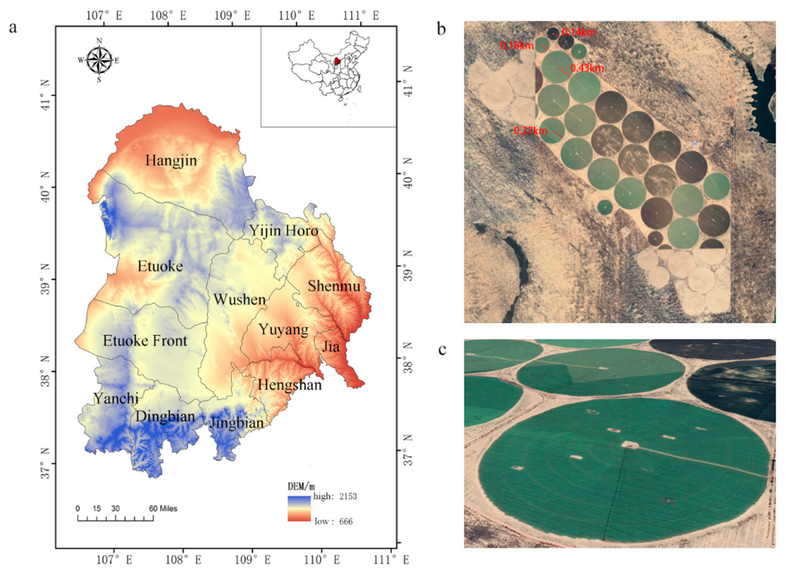
The Mu Us region is situated in the northwestern area of China, encompassing the northern parts of Yulin City in Shaanxi Province, the northern parts of Wuzhong City in Ningxia Hui Autonomous Region and the southern parts of Ordos City in Inner Mongolia Autonomous Region (36°48′–40°52′N, 106°28′–110°54′E). The region spans 12 counties (banners) and covers a total area of approximately 100,000 km2 (Figure 1a). The region falls with the temperate continental monsoon climate, with an annual precipitation gradient that decreases from southeast to northwest, ranging from 250 mm to 440 mm. The CPI system represents the primary agricultural production method in the Mu Us region in recent times, documented in Figure 1b,c; it is an irrigation approach employing a rotating tower-supported radial pipe to evenly distribute water onto crops.

Figure 1.
The geographical location of Mu Us region. ((a) Administrative division and geographical location of Mu Us region; (b) satellite image illustrating the different size classes of CPI farmlands in Mengjiawan (38.653°N, 109.605°E); (c) CPI farmland near-ground image in Mengjiawan. The base map was derived from Google Earth).
2.2. Data Sources
The NDVI data were obtained from the MOD13Q1 data, which had a spatial resolution of 250 m and a temporal resolution of 16 days, and two images were accessible every month. The analysis was restricted to the growing season, which was defined as April to October in the Mu Us region [28,29]. To reduce the noise in the NDVI data, which may be caused by cloud cover, the monthly NDVI was calculated on the Google Earth Engine (GEE) platform using the maximum value synthesis method. Subsequently, annual NDVI data were obtained using the mean method [30,31]. Pixels with an annual NDVI below 0.05 were excluded from this study as non-vegetated areas, in accordance with previous studies [32,33].
The land use data originated from the China Land Cover Annual Dataset (CLCD), which used the GEE platform to collect all available Landsat data and generated land use classification results by constructing spatiotemporal features and combining random forest classifiers [34]. CLCD is among the primary land use datasets in China, with elevated spatial resolution and classification precision [35].
The temperature and precipitation data were obtained from the “China Surface Climate Data Daily Dataset (V 3.0)” of the China Meteorological Data Sharing Service Network. Stations with complete data from 2008 to 2019 were selected, and the daily data were aggregated into annual data, calculating two indicators: annual mean temperature and annual total precipitation. Using ANUSPLIN4.1 software, elevation information was introduced as a covariate, and spatial interpolation was performed on these two climatic factors to generate raster data with a resolution of 30 m.
The data for total terrestrial water storage was obtained from the Mass Concentration data released by the Center for Space Research at the University of Texas at Austin. In instances where data gaps occurred, singular spectrum analysis (SSA) was employed to interpolate [36]. Furthermore, in order to determine groundwater fluctuations in the study area, a water balance equation was formulated:
In the equation, ΔTWS is the total water storage change provided by Mass Concentration, ΔGWS is the groundwater storage change, Δsoil is the soil water change, and Δcanopy is the vegetation water change. Vegetation water and soil water data were extracted from the Global Land Data Assimilation System.
3. Method
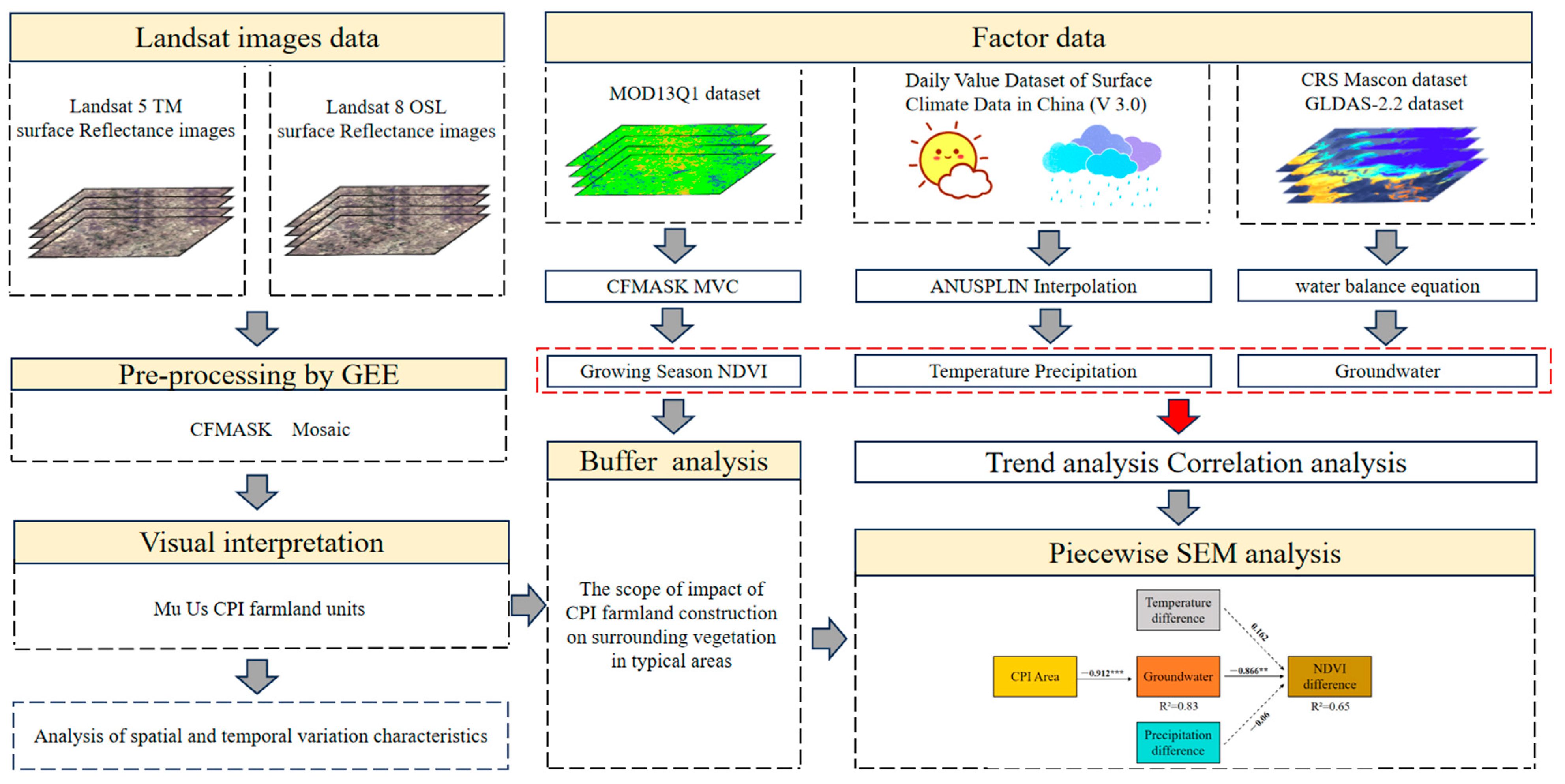
This study consists of four main steps: (1) using visual interpretation of Landsat images to extract annual CPI farmland units data from 2008 to 2022; (2) analyzing the spatiotemporal characteristics of CPI farmland units based on multi-year data; (3) setting buffer zones to analyze the impact range of CPI farmland unit construction on the surrounding vegetation in typical areas; (4) establishing SEM to analyze the impact mechanism of CPI farmland unit construction on the surrounding vegetation growth in the study area. The detailed workflow is shown in Figure 2.

Figure 2.
Technical flow chart of the study. The significance levels of each predictor are ** p < 0.01, *** p < 0.001.
3.1. CPI Farmland Extraction
The annual CPI farmland unit data from 2008 to 2022 were obtained by visual interpretation of Landsat (TM/ETM+/OLI) images with a spatial resolution of 30 m. The Landsat images were downloaded from the GEE platform, which provided Landsat SR remote sensing image data that had been atmospherically corrected and radiometrically calibrated. The images were then cloud-removed and mosaic-processed for visual interpretation. The active cultivation of crops made the CPI farmland unit easier to identify, so the remote sensing images were mostly selected in the growing season.
3.2. Mann–Kendall Trend Test
The Mann–Kendall trend test is a non-parametric test method recommended by the World Meteorological Organization, which is widely used worldwide by many scholars to analyze the changes of time series such as temperature, precipitation, runoff, etc. [37,38].
We compared the given time series data x in sequence, and the result is recorded as sgn(xi − xj) = sgn(θ):
Mann–Kendall statistical parameters S and variance are defined as follows:
In the formula, xj and xk are random variables, and j and k are integers from 1 to n and satisfy j > k.
In the equation, Z is the statistic, Z > 0 indicates an upward trend in the data series, Z < 0 indicates a downward trend in the data series, |Z| ≥ 1.96 indicates a significant change trend, and |Z| ≥ 2.58 indicates a very significant change trend.
3.3. Pearson Correlation Analysis
The Pearson correlation coefficient can be used to express the degree of correlation between two sets of variables. In this study, this coefficient was used to analyze the correlation between the total CPI farmland area, NDVI data, temperature, precipitation, and groundwater storage. The calculation formula is as follows:
In the formula, r is the correlation coefficient between variables x and y; xi and yi are the data of two factors in a certain year, respectively; x and y are the average values of two factors in many years, respectively; for the correlation coefficient value [−1, 1], the greater the absolute value of the correlation coefficient, the stronger the correlation, and vice versa. We used the t test to verify the significance of the correlation.
3.4. Typical Regional Buffer Analysis
The principles for selecting typical areas are (1) CPI farmland units have a long sprinkler irrigation time, have been irrigated for many years and have not been abandoned, resulting in a strong ecological effect; (2) they can be composed of one or several CPI farmland units, but after they are built, there are no new CPI farmland units added in their 5 km buffer zone in the subsequent time, ensuring that they are not affected by the cross-effect of multiple CPI farmland units; and (3) there are no impermeable surfaces or more cultivated land in the buffer zone, avoiding the impact of other human activities on vegetation growth.
In this study, two typical regions were selected (Figure 3), namely typical area 1 (TA1, 38°34′1″–38°43′23″N; 109°26′41″–109°42′33″E) and typical area 2 (TA2, 38°18′41″–38°17′48″N; 108°45′45″–108°46′32″E). The CPI farmland units in TA1 and TA2 were built in 2015, consisting of 45 and 5 CPI farmland units, respectively. In order to analyze the impact of CPI farmland unit construction on the vegetation growth in the typical area, we used buffer zone analysis method to compare the NDVI change trends in each buffer zone. Considering the size of CPI farmland unit and the spatial resolution of NDVI data, we drew a circular ring as a buffer zone every 500 m from the center of CPI farmland unit, with a total of 10 buffer zones, which were named as Buffer1–Buffer10 according to their distance from CPI farmland unit.
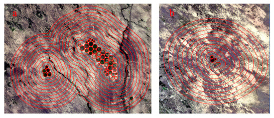
Figure 3.
Real images of the surface of the typical area. ((a) TA1; (b) TA2).
3.5. Propensity Score Matching
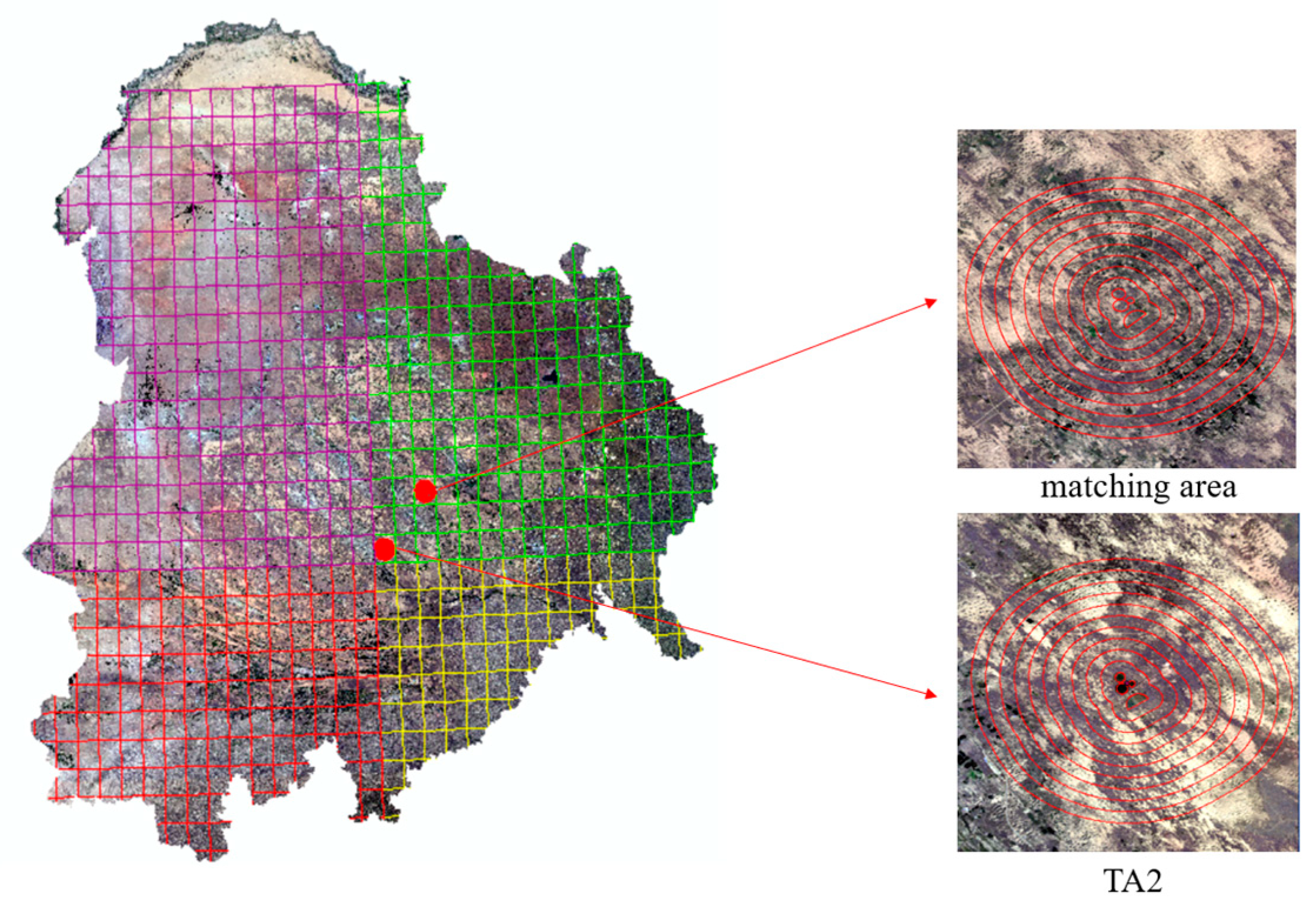
To verify whether the construction of CPI farmland units has an impact on the vegetation growth around them, we use the propensity score matching method to select areas with similar temperature and precipitation as the matching area and conduct a comparative analysis. The specific steps are as follows: (1) We draw a square around TA 2, so that TA 2 and its buffer zone are completely within the square. Using the fishnet tool of Arcgis, we divide the Mu Us region into equal-sized square grids, with the square of TA 2 as the coordinate center. (2) Using the propensity score matching method, we find the grid that is most similar to TA 2 in terms of temperature, precipitation, terrain, etc. (3) In the second step, we draw a buffer zone with the same area as TA 2 in the matched grid (Figure 4). The reason for choosing the TA 2 for propensity score matching is that it has a small area and is easier to find similar areas.

Figure 4.
Propensity score matching method matches similar areas.
3.6. Structural Equation Model
In order to investigate the mechanism of the impact of CPI farmland construction on the differences in the growth of surrounding vegetation, two buffer zones of 500–3000 m and 3000–5000 m were set up based on the 2019 CPI farmland data, and the changes in their air temperature, precipitation, NDVI and groundwater reserves were calculated from 2008 to 2019, respectively. Piecewise Structural Equation Model [39] was used to explore how changes in air temperature, precipitation and groundwater storage affect the impact of CPI farmland construction on the growth of surrounding vegetation. The NDVI, temperature and precipitation are the annual differences within the two buffer zones, and the groundwater storage change value is the annual average within the two buffer zones. The NDVI difference calculation formula is as follows:
In the formula, NDVID is the difference between the two buffer zones, NDVIB1 and NDVIB2 are the mean values of NDVI in the 500–3000 m and 3000–5000 m buffer zones, respectively, and i represents the year. The above formula also applies to the temperature difference and precipitation difference.
All data subjected to SEM analyses were divided by the corresponding standard deviation to keep data volumes on the same scale. The superiority of model fit was assessed using Fisher’s C statistic [40], and all statistical analyses were performed using R4.3.1.
4. Results
4.1. Temporal and Spatial Variation Characteristics of CPI Farmland Units in Mu Us Area
4.1.1. Time Changing Characteristics
From 2008 to 2022, the number and area of CPI farmland units in the Mu Us region showed a continuous increasing trend and did not reach the peak (Figure 5a). The changes in CPI farmland unit number and area can be divided into three stages: (1) A slow growth period (2008–2012) from the first appearance in 2008 to 2012, where the number and total area of CPI farmland units were only 309 and 52.64 km2. (2) A rapid growth period (2013–2017) from 2013, where the number and total area of CPI farmland units increased rapidly, with 803 and 111.41 km2 added in 2014 alone, reaching 3306 and 472.83 km2 in 2017. (3) A decelerated growth period (2018–2022) from 2018, where the number and total area of CPI farmland units continued to increase but at a slower pace, with the lowest number and area added in 2018 being only 171 and 17.42 km2 and an average of about 400 and 30.44 km2 added annually from 2019 to 2022, reaching 4829 and 641.61 km2 in 2022 and possibly continuing the increasing trend.
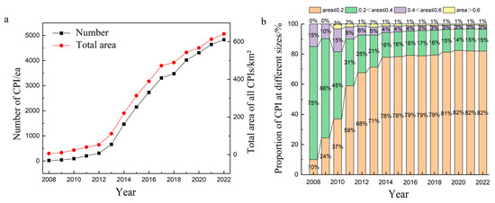
Figure 5.
Change trend of CPI farmland units. ((a) Number and growth trend of CPI farmland units; (b) proportion of CPI farmland units of different sizes).
According to the area of CPI farmland units, it can be divided into four scales: small (0–0.2 km2), medium (0.2–0.4 km2), large (0.4–0.6 km2) and huge (>0.6 km2). In 2008, medium-sized CPI farmland dominated, accounting for 75%. Subsequently, the proportion of medium and large CPI farmland units gradually decreased, while the proportion of small CPI farmland gradually increased. After 2014, the proportion of various scales of CPI farmland units was basically stable, with the combined proportion of small and medium-sized reaching up to 95%, and the combined proportion of large and huge being only 5% (Figure 5b).
4.1.2. Spatial Variation Characteristics
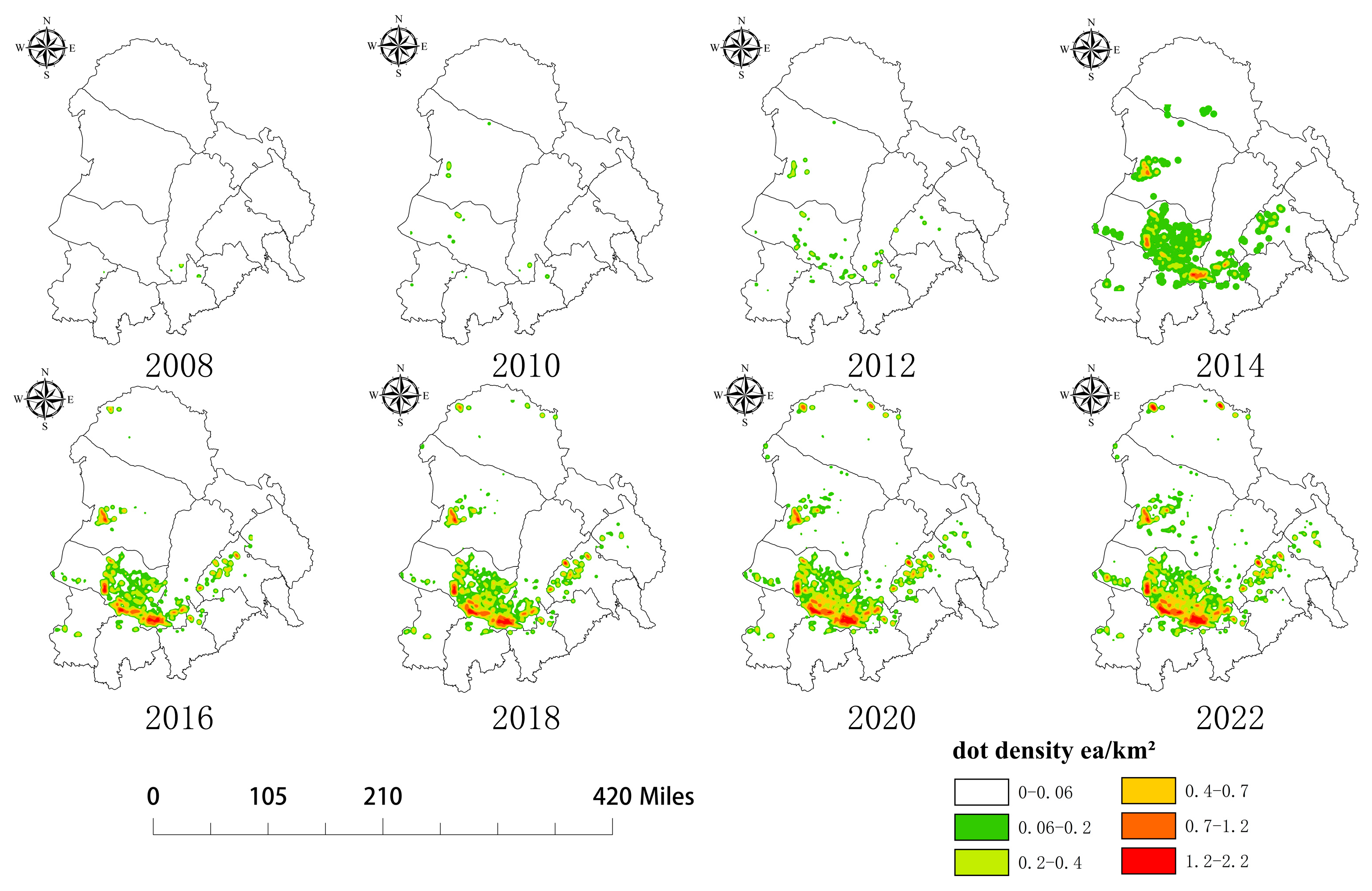
The spatial distribution and development changes of CPI farmland units in the Mu Us region are shown in Figure 6. From 2008 to 2012, there were few CPI farmland units in the Mu Us region, which were only distributed in some areas of Etoke Banner, Etoke Front Banner, Wushen Banner, Yuyang District and Jingbian County. From 2014, the number of CPI farmland units increased sharply, mainly concentrated in Etoke Front Banner. After 2016, CPI farmland units formed a spatial pattern with Etoke Front Banner as the core and Etoke Banner, Yuyang District and Wushen Banner as the support.
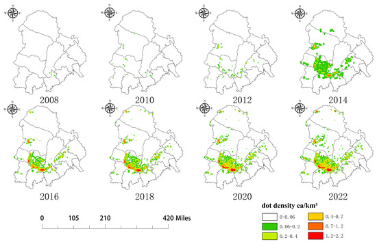
Figure 6.
Spatial distribution of CPI farmland unit hotspots every two years from 2008 to 2022.
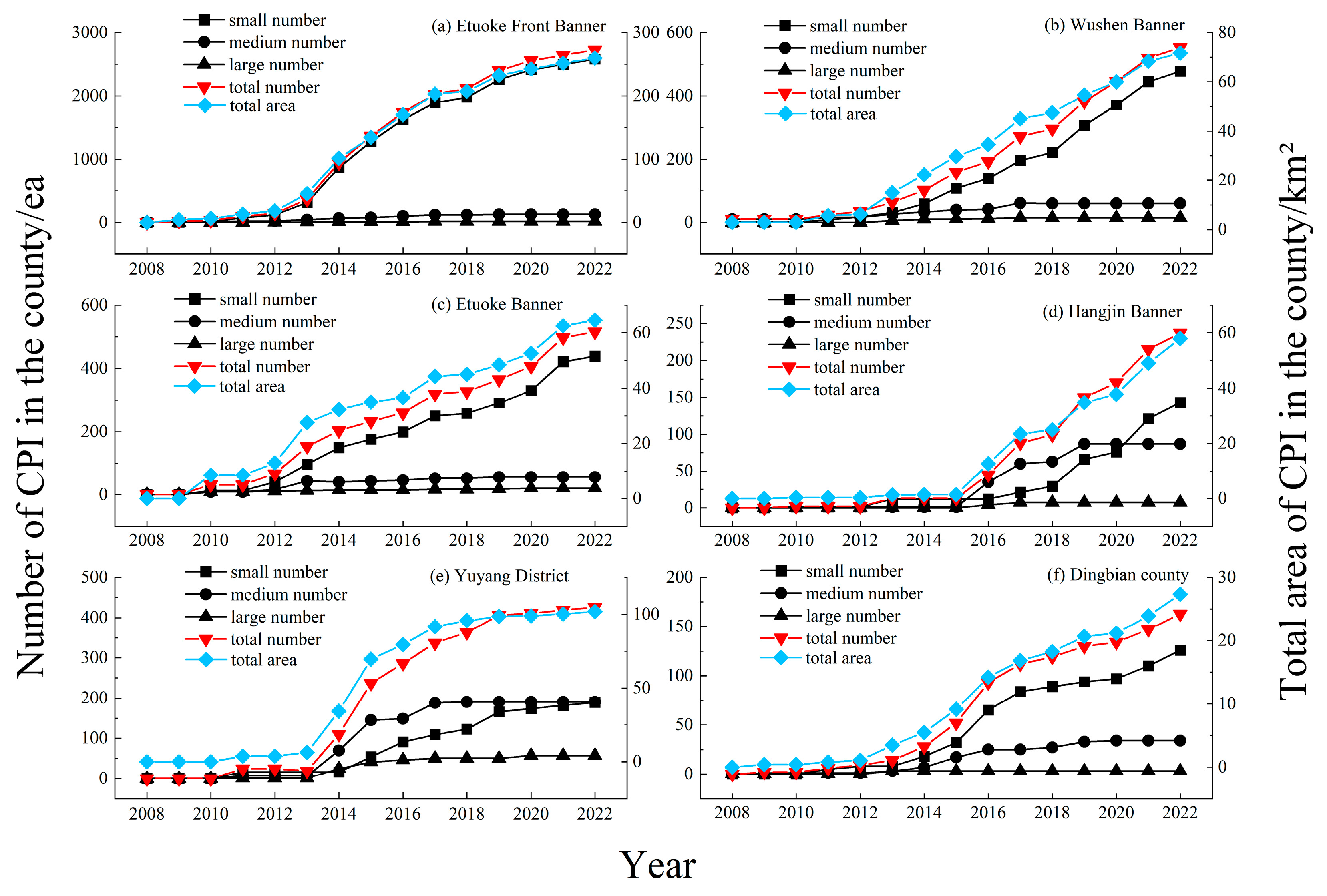
4.1.3. Analysis of Changes in CPI Farmland Units in Each County
The number, area and scale of CPI farmland units in each county of the Mu Us region vary greatly (Figure 7). From the perspective of CPI farmland unit number and area change trends, Etoke Front Banner experienced rapid growth from 2013 to 2017, but the growth rate has slowed down since 2018. By 2022, the number of CPI farmland units in this banner reached 2727, with a total area of 259.75 km2, which is the county with the largest number and area of CPI farmland units in the study area. The number and area of CPI farmland units in Wushen Banner, Etoke Banner and Hangjin Banner showed a continuous increasing trend, among which, the construction of CPI farmland units in Hangjin Banner started in 2016, relatively late, and the number and area were relatively small. Yuyang District experienced rapid growth from 2014 to 2015, gradually slowed down from 2017 to 2019 and almost no growth after 2020. Dingbian County experienced rapid growth from 2013 to 2016, slowed down from 2017 to 2020 and strengthened its growth momentum from 2021 to 2022. From the perspective of scale change, Etoke Front Banner, Wushen Banner, Etoke Banner and Dingbian County were dominated by small-scale CPI farmland units, and there were relatively few medium and large-scale CPI farmland units. Hangjin Banner and Yuyang District both started with the construction of medium-sized CPI farmland units, with concentrated construction time from 2016 to 2019 and from 2014 to 2017, respectively, and no growth afterwards. By 2022, the number of medium-sized CPI farmland units accounted for 43.5% and 36.7% of the total number in the two places, respectively. The number of large-scale CPI farmland units was very small, concentrated in Yuyang District.
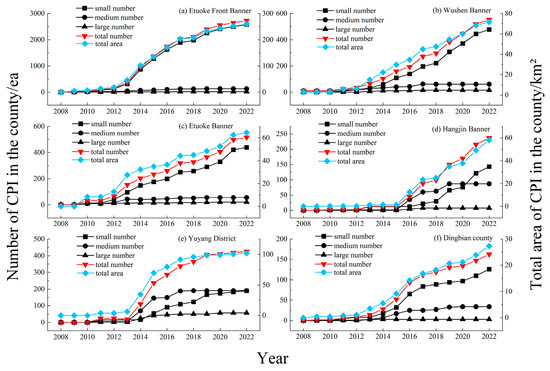
Figure 7.
CPI farmland unit change trend of each county in Mu Us prefecture from 2008 to 2022. (Note: the figure only shows counties with more than 100 CPI farmland units by 2022; because the number of giant CPI farmland units is very small, they are counted as large CPI farmland units during calculation).
4.1.4. Land Use Analysis
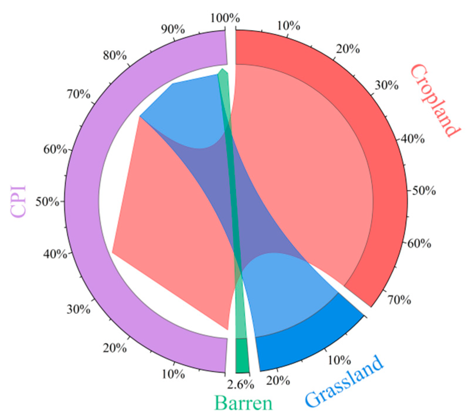
To explore the conversion relationship between CPI farmland and other land use types in the Mu Us region, we overlaid the data of newly added CPI farmland each year with the land use data of the previous year, and the results were drawn as a chord diagram (Figure 8). The formation of CPI farmland mainly involved the conversion process of cultivated land, grassland and wasteland. Among them, the conversion area of cultivated land was the largest, reaching 475.3 km2, accounting for 74% of the total amount of CPI area transferred. The second was grassland, with a conversion area of 149.5 km2, accounting for 23.4% of the total amount of CPI area transferred. The conversion area of wasteland to CPI farmland was the smallest, only 16.8 km2, accounting for 2.6% of the total amount of CPI area transferred.

Figure 8.
Proportion of CPI farmland land types transferred into.
4.2. Typical Area Analysis
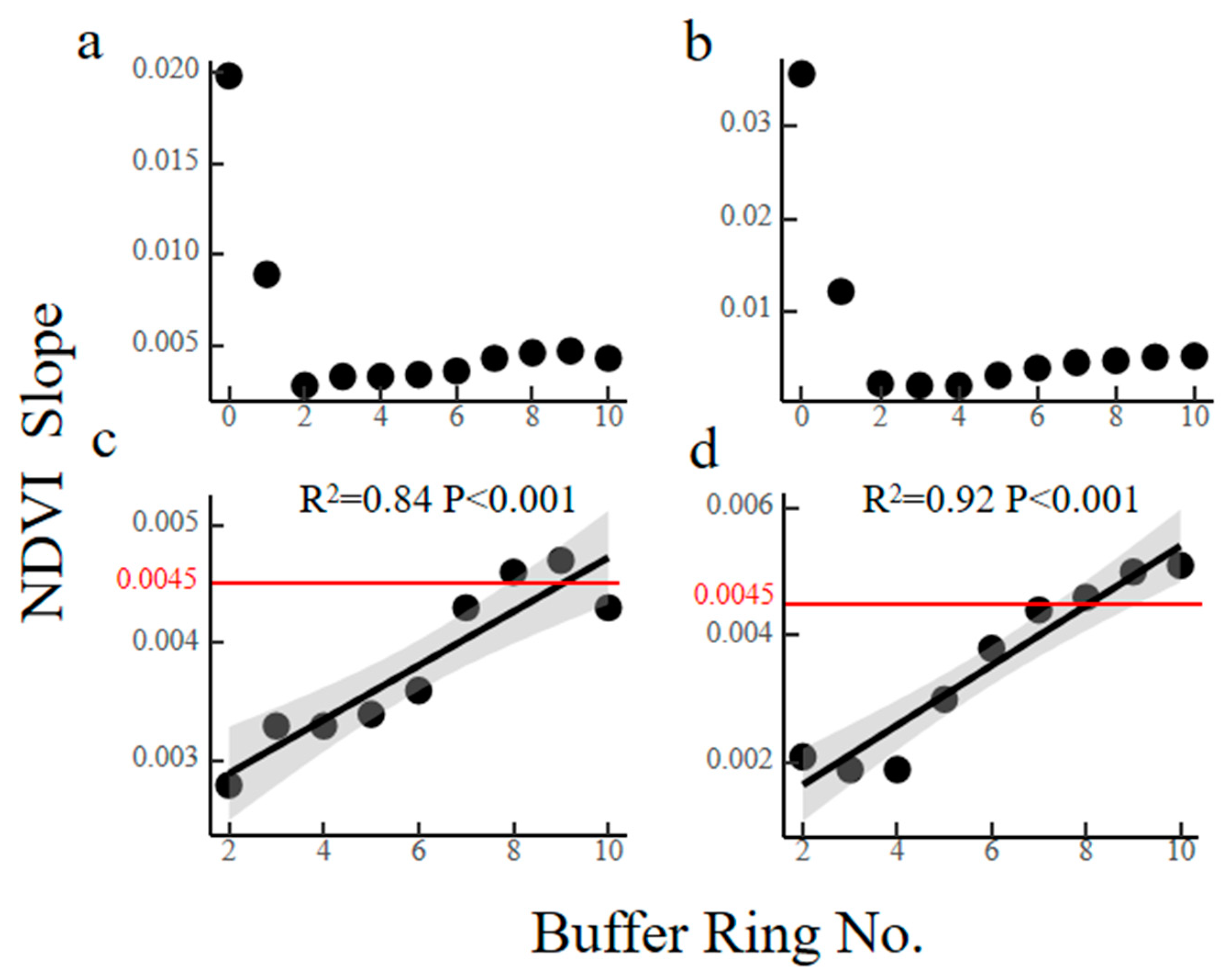
In TA1 and TA2, NDVI increased significantly with the construction age of CPI farmland units in the interior of CPI farmland, Buffer1 and Buffer6–Buffer10, while NDVI did not increase significantly with the construction age of CPI farmland units in Buffer2–Buffer5 (Figures S1 and S2). In TA1 and TA2, the NDVI change rate of CPI farmland and Buffer1 both exceeded the average level of 0.0045/a in the Mu Us region (Figure 9a,b). The NDVI change rates of CPI farmland units and Buffer1 in TA1 were 0.0198/a and 0.0091/a, respectively, which were four and two times higher than the average level of the Mu Us region. The NDVI change rates of CPI farmland units and Buffer1 in TA2 were 0.0375/a and 0.0121/a, respectively, which were eight and two times higher than the average level of the Mu Us region.
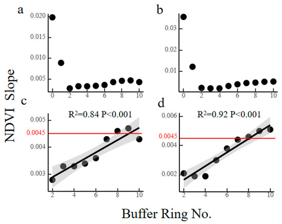
Figure 9.
The spatial trend of annual NDVI changes. ((a,b) The trend of NDVI changes in CPI farmland units and Buffer1–Buffer10 of TA1 and TA2 from 2015 to 2022; (c,d) the regression analysis of the buffer distance and the NDVI change trends in TA1 and TA2).
In the buffers from Buffer2 to Buffer10, the NDVI change trend increased with the distance from the CPI farmland (Figure 9c,d). This pattern was consistent in TA1 and TA2. Among the buffers, the NDVI change trends of Buffer2–Buffer6 were lower than the average level of the Mu Us region, while the NDVI change trends of Buffer7–Buffer10 were close to the average level of the Mu Us region. To verify whether the above pattern was caused by the construction of CPI units, we used the propensity score matching method to select a similar area for verification. The results showed that the NDVI change trend of each buffer zone in the matching area was around 0.0045/a, and that the NDVI change trends of Buffer2–Buffer6 were not lower than those of Buffer7–Buffer10 (Figure S3). This indicates that the construction of CPI farmland units indeed inhibits the NDVI increase in Buffer2–Buffer6.
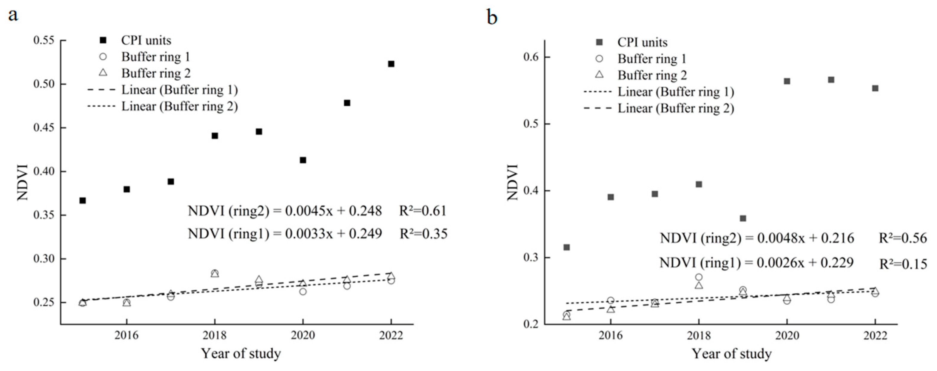
The regression analysis of the mean NDVI values in Buffer2–Buffer6 and Buffer7–Buffer10 with the construction age of CPI farmland units showed that the NDVI change trends of Buffer7–Buffer10 were significantly higher than that of Buffer2–Buffer6. In TA1, the NDVI change trends of Buffer2–Buffer6 and Buffer7–Buffer10 were 0.0045/a and 0.0033/a, respectively, while in TA2, they were 0.0048/a and 0.0026/a (Figure 10).

Figure 10.
NDVI change trends of CPI farmland units, ring1 and ring2. ((a) TA1; (b) TA2. Note: ring1 refers to the mean NDVI of Buffer2–Buffer6, ring2 refers to the mean NDVI of Buffer7–Buffer10).
4.3. Impact Mechanism Analysis
4.3.1. Characteristics of Climate, Groundwater and Vegetation Changes
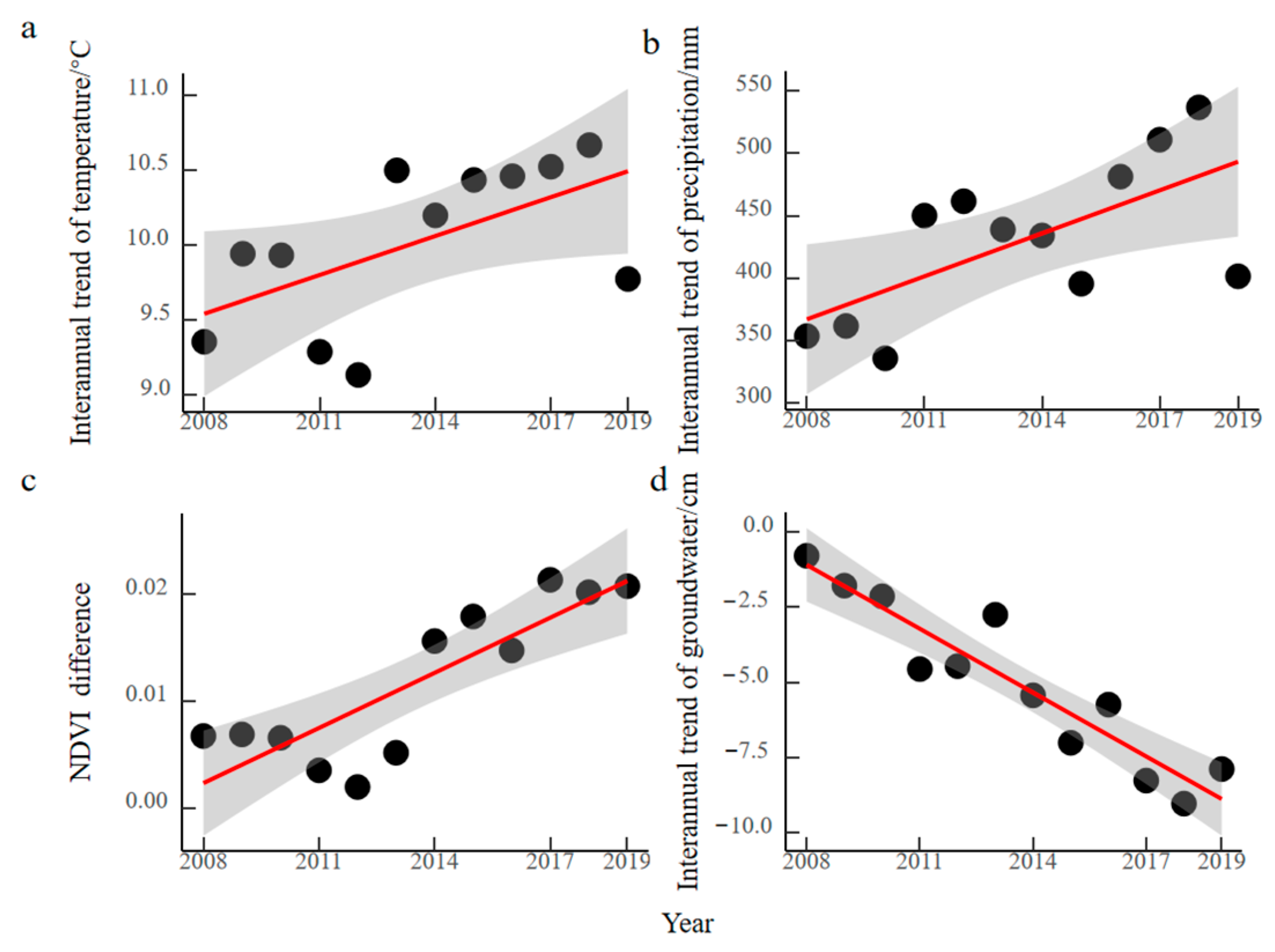
During 2008–2019, temperature, precipitation and NDVI difference within the 5000 m buffer zone of CPI farmland in Mu Us region all showed an increasing trend, while groundwater storage showed a decreasing trend (Figure 11). The temperature increase was not significant, with a change rate of 0.08 °C/a (p < 0.05) and a total increase of about 0.9 °C. The precipitation increase was significant, with a change rate of 13 mm/a (p < 0.05); although, there were some years with a precipitation reduction, but the overall trend was obvious. The NDVI difference gradually narrowed from 2008 to 2012, but expanded rapidly after 2013, with a change rate of 0.0003/a (p < 0.05). Among them, the increase in 2014 was the highest, reaching 0.001, which is noteworthy that this year was also the year with the most CPI farmland increase. The groundwater level change showed a continuous downward trend from 2008 to 2019 (−0.71 cm/a, p < 0.01), with a total drop of about 10 cm.
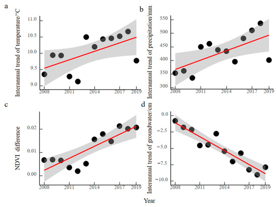
Figure 11.
Interannual variation trends. ((a) Temperature; (b) precipitation; (c) NDVI differences; (d) groundwater).
4.3.2. Impact on the Growth of Surrounding Vegetation
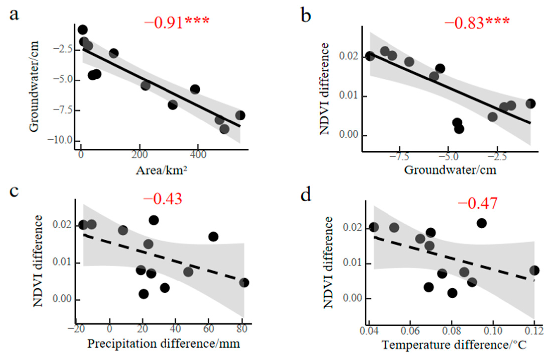
To find the factors related to the increase in NDVI difference between 500 and 3000 m and 3 and 5 km in the Mu Us region, we selected the changes in groundwater storage, temperature difference and precipitation difference for the correlation analysis. Both temperature difference and precipitation difference were the differences between 500 and 3000 m and 3000 and 5000 m. The correlation analysis showed that the change in groundwater storage was significantly negatively correlated with the total area of CPI farmland, and the NDVI difference was significantly negatively correlated with the change in groundwater storage, while there was no significant correlation with the temperature difference and precipitation difference (Figure 12).
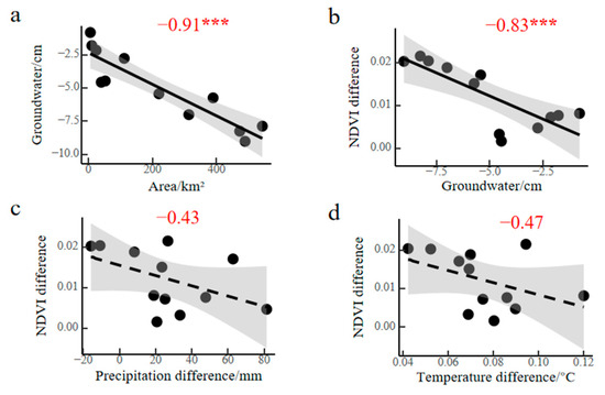
Figure 12.
Correlation analysis. ((a) Correlation analysis of CPI farmland area and groundwater storage change; (b) correlation analysis of NDVI difference and groundwater storage change; (c) correlation analysis and NDVI difference and precipitation difference; (d) correlation analysis of NDVI difference and temperature difference. The significance level of predictor is *** p < 0.001).
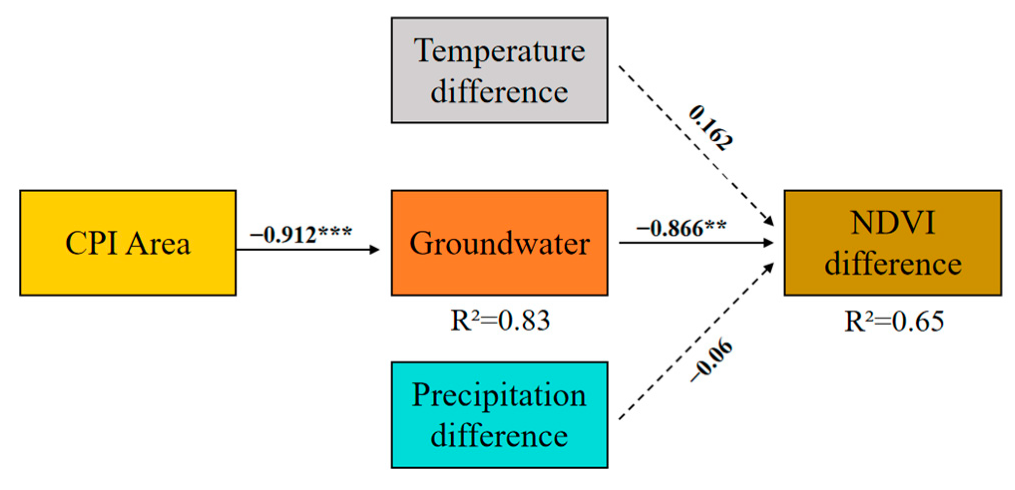
The structural equation model had a good fit (Fisher’s C = 10.449, df = 6, p = 0.11), and the relationships among the variables were effectively expressed (Figure 13). The increase in CPI farmland area would significantly enlarge the NDVI difference between 500 and 3000 m and 3000 and 5000 m, which was mainly achieved by consuming groundwater storage. The effects of temperature and precipitation on NDVI difference were not significant. The mediation effect of CPI farmland expansion on NDVI difference was 0.789, and the effects of temperature difference and precipitation difference were 0.162 and −0.06, respectively. The total effect could explain 65% of the variation in NDVI difference (R2 = 0.65).
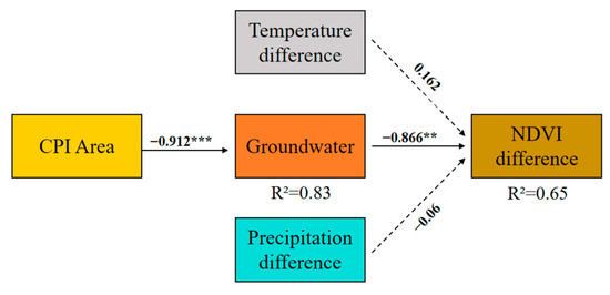
Figure 13.
Attribution analysis of NDVI difference (Note: The significance levels of each predictor are ** p < 0.01, *** p < 0.001).
5. Discussion
5.1. Current Status of CPI Farmland Units Construction in Mu Us Area
The number and area of CPI farmland units in the Mu Us region are in a continuous growth stage, with small-scale CPI farmland units as the main scale, which is consistent with the previous research results [41]. Initially, the Mu Us region tried to promote the construction of large-scale CPI farmland units, but the actual results showed that large-scale CPI farmland units did not achieve effective promotion, but small-scale CPI farmland units were favored by farmers, which mainly benefited from the support of local projects [42,43]. The CPI farmland units in the Mu Us region are mainly distributed in Ordos City and Yulin City, with Ordos City as the main development area. In Ordos City, the construction of CPI farmland units is a demonstration project of the one million modern agriculture construction project in Inner Mongolia, which is responsible for construction and operation by local farmer–herder cooperatives or mutual aid groups. The sprinkler irrigation equipment is jointly invested in by the national and local governments, with a relatively small-scale and discrete distribution, with an average of about 0.13–0.2 km2 per operation area. In Yulin City, with the help of the cultivated land occupation and compensation balance fund of Shaanxi Province, the modern agricultural park project is adopted for corporate development and construction, and the CPI farmland units shows a contiguous distribution with a relatively large scale.
5.2. Future Growth Trend of CPI Farmland Units in Mu Us Area
In recent years, the growth trend of CPI farmland unit number and area in each county of the Mu Us region shows that some counties in Yulin City have experienced growth stagnation, and the overall growth rate is very low, while most areas in Ordos City still maintain a continuous growth momentum. Yulin City is water-scarce, although there is data showing that groundwater storage is abundant in the Mu Us region (Yulin City) [44], but due to a low utilization rate and large-scale land reclamation and development, the groundwater level has dropped significantly [45]. Recently, Yulin City issued the “Development Plan for Building Shaanxi Modern Agriculture Leading Zone in the 14th Five-Year Plan Period”, which will gradually replace sprinkler irrigation technology with drip irrigation technology as the main means to promote efficient dryland water-saving agriculture. Ordos City issued the “Implementation Opinions of Ordos Municipal People’s Government on Further Strengthening High-standard Farmland Construction and Enhancing National Food Security Guarantee Capacity”, which emphasized continuing to promote high-standard farmland construction mainly based on sprinkler irrigation. Affected by the different water resources and local policies of the two places, it is expected that the number and area of CPI farmland units in Ordos City will continue to increase in the future, while Yulin City may show a trend of stopping growth or even decline.
5.3. Problems Existing in CPI Farmland Units in Mu Us Area
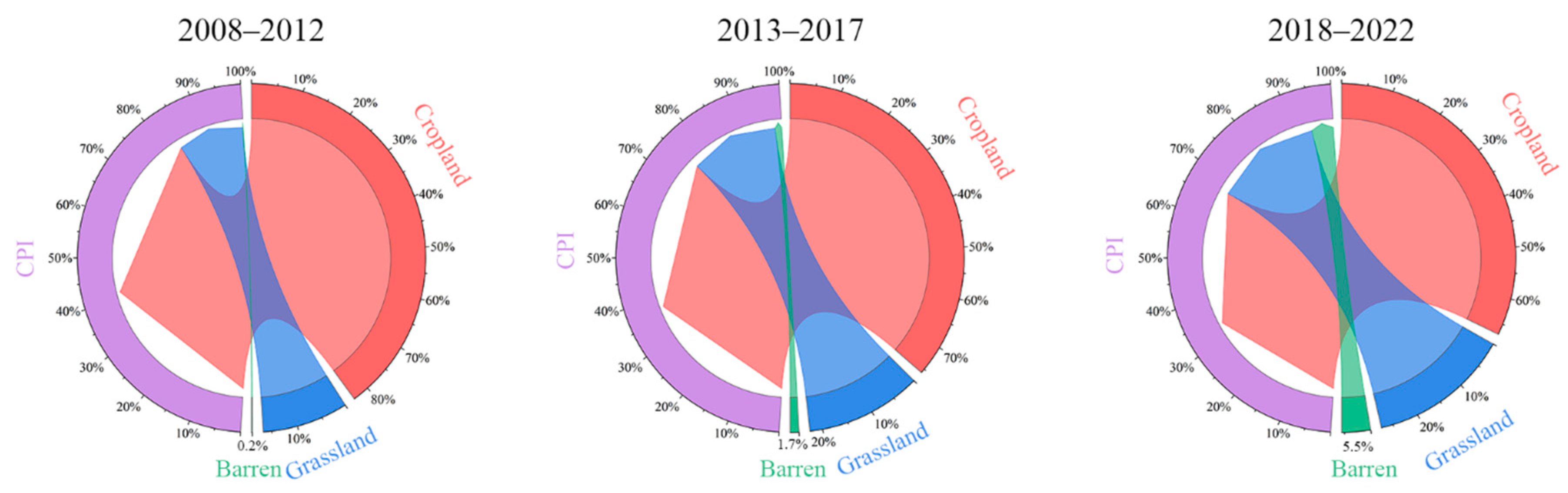
CPI farmland in the Mu Us region mainly came from the conversion of three land use types, cultivated land, grassland and wasteland, among which cultivated land was the main one (Figure 8). According to the growth trend of CPI farmland in the Mu Us region (Figure 5), we analyzed the proportion of land use types transferred to CPI farmland in three stages (Figure 14). The results showed that over time, although cultivated land still dominated, its proportion was gradually decreasing, while the proportion of grassland and wasteland was gradually increasing. This means that the area of cultivated land available for constructing CPI farmland is gradually decreasing, and the expansion of CPI farmland will inevitably increase the reclamation of grassland and wasteland. However, CPI farmland construction mainly considered its economic benefits, without considering its dual effects of economy and ecology. Most herbaceous plants still have their root systems after defoliation in winter [46], which can effectively reduce soil loss [47], thus playing a positive role in inhibiting land desertification. Within CPI farmland, forage corn and potatoes are mainly planted. After harvesting in autumn, their root systems also die, and the plowed sand is completely exposed, with no vegetation cover on the surface (Figure 15a,b) until the seedlings emerge after sowing in the next spring, lasting for about 6 months, during which there is a high possibility of wind and sand dust. In addition, there is also a lack of shelterbelt system construction near CPI farmland, even if a few trees are planted around some cultivated land, but they do not meet the standard of farmland shelterbelt in terms of scale and distribution (Figure 15c,d). With more and more grassland reclaimed as CPI farmland, it may aggravate the local land desertification problem.
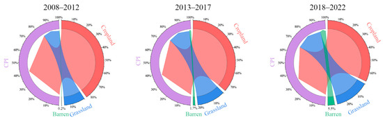
Figure 14.
Proportion of CPI farmland land types transferred in three stages (2008–2012, 2013–2017, 2018–2022).
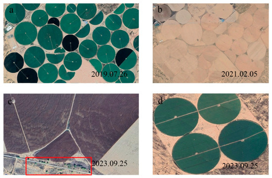
Figure 15.
CPI farmland unit image from Google Earth. ((a) CPI farmland image during the growing season; (b) CPI farmland image during the non-growing season; (c,d) CPI farmland surrounding images. Note: 1. The remote sensing image data source in Google Earth comes from Landsat. 2. Marked in the red box are the protective forests near CPI farmland units).
5.4. Impact of CPI Farmland Unit Construction on Surrounding Vegetation Growth in Typical Areas
The study of the typical region found that the NDVI increasing trend within the CPI farmland units was higher due to continuous irrigation and no abandonment, while the surrounding buffer zones were relatively lower. However, the NDVI increasing trend in Buffer1 was also faster. On the one hand, it may be due to excessive irrigation, resulting in water outflow and forming small runoff [48,49], which promoted the growth of surrounding vegetation; on the other hand, when being visually interpreted, the CPI units were circular, which caused some extraction errors, and some parts that belonged to CPI units were not completely extracted, which was equivalent to increasing the NDVI within Buffer1. The NDVI values in Buffer2–Buffer5 did not increase significantly with time, while Buffer6–Buffer10 increased significantly, which may be related to the change in groundwater level. The excessive extraction of groundwater would cause land subsidence [50,51], which would affect the surrounding vegetation [52], and this effect would weaken as it was farther away from CPI farmland units. The phenomenon that the NDVI change trend in Buffer2–Buffer10 gradually increased also seemed to confirm this point. In addition, in the Mu Us region, vegetation was mainly perennial herbs [53,54,55,56], and the proportion of annual and perennial plants in the buffer zone would also affect the NDVI change trend.
We also found that the temporal patterns of NDVI in all buffer zones in TA1 and TA2 are similar, which seems to be influenced by some environmental factors. We used a random forest model to examine the relationship between the growing season NDVI value, as the dependent variable, and three factors that are closely related to vegetation growth, as independent variables, namely temperature, precipitation and groundwater change. Then, we used the sobol global sensitivity analysis method to find out the environmental factor that has the greatest impact on vegetation NDVI (Table S1). The results of the sensitivity analysis show that temperature is the main factor affecting the vegetation NDVI in TA1 and TA2. This is consistent with previous studies. On the larger scale of the Yellow River basin compared to the Mu Us region, Li et al. [57] found that temperature was the main factor affecting the vegetation growth change on the temporal scale, through correlation analysis and factor detection analysis. Zhao et al. [58] also found that temperature was the main factor affecting NDVI in the Heihe River basin, based on the study of the relationship between meteorological factors and NDVI.
5.5. The Impact of CPI Farmland Units Construction on Vegetation Growth
The SEM results showed that the increase in CPI farmland area led to the decrease in groundwater storage, which became the main factor inhibiting the vegetation growth in the buffer zone of 500 m to 3000 m. Chen et al. [59] used trend analysis and spatial correlation method to study CPI farmland units in Ulanqab City and found that the groundwater cone of depression caused by CPI farmland units construction led to vegetation degradation within 10,000 m, and the farther away from CPI farmland units, the smaller this degradation effect. At present, there is no obvious vegetation degradation effect near CPI farmland units in the Mu Us region, but it has produced a significant inhibitory effect, and the impact range is smaller than that in Ulanqab City. The reason for this difference may be related to the groundwater depth and storage in the two places. The groundwater in the Mu Us region is buried deep and has abundant storage [60], and the groundwater storage decreased by about 10 cm in the past 20 years, while the groundwater in Ulanqab City is buried shallow and has relatively less storage, and the groundwater level dropped by about 2 m from 2015 to 2018 [59]. Therefore, for the Mu Us region, the continuous expansion of CPI farmland units resulted in a relatively mild situation of groundwater cone of depression, and its impact range was limited to about 3000 m near CPI farmland units. However, the impact range of 3000 m is only applicable to the overall CPI farmland units in the Mu Us region, and the aggregation degree of CPI farmland units may affect this range. For example, when there are a limited number of CPI farmland units in a large area, its impact on the surrounding vegetation growth may be small or even insignificant; when there are many CPI farmland units in a small area, its impact range may exceed 3000 m. In addition, the hydrogeological conditions of different regions will also have an impact on this range. With the continuous expansion of CPI farmland units and the increase in sprinkler irrigation time, groundwater consumption may further intensify, which may also lead to the expansion of impact range, or even cause problems such as vegetation degradation.
6. Conclusions
CPI farmland units in the Mu Us region started to be built in 2008, and the number and area change trend can be divided into three stages: a slow growth period from 2008 to 2013, a rapid growth period from 2013 to 2017, and a decelerated growth period from 2017 to 2022. The construction scale of CPI farmland units were mainly small and medium-sized CPI farmland units, and large-scale CPI farmland units were mainly distributed in Yuyang District. From the perspective of spatial change, Etoke Front Banner was the focus of CPI farmland unit construction in the study area and showed a trend of expanding outward.
The number and area of CPI farmland units in Yulin City grew slowly, while those in Ordos City maintained a continuous upward trend. Affected by water resources and policies, CPI farmland units in Ordos City may continue to increase in the future, while it may stop growing or even show a downward trend in Yulin City.
CPI farmland unit construction destroyed natural vegetation, causing land desertification to some extent. Therefore, wind and sand control measures should be paid attention to in the construction of the protection system, and standardized management should be carried out.
Within the typical region, CPI farmland unit construction had a promoting effect on the vegetation within it and within the 500 m buffer zone, an inhibitory effect on the vegetation within the 500–3000 m buffer zone, and no significant effect on the vegetation within the 3000–5000 m buffer zone.
The main factor inhibiting the vegetation growth in the CPI farmland units buffer zone of 500–3000 m in the Mu Us region is the overexploitation of groundwater, rather than the meteorological factors.
Supplementary Materials
The following supporting information can be downloaded at: https://www.mdpi.com/article/10.3390/rs16030569/s1, Figure S1: Changes in value of NDVI in each buffer zone of CPI farmland in TA1 from 2015 to 2022. (a): CPI internal; (b–k): Buffer1-Buffer10. The solid line indicates a significant effect and the dotted line indicates no significant effect, as will be the case in subsequent analyses; Figure S2: Changes in value of NDVI in each buffer zone of CPI farmland in TA2 from 2015 to 2022. (a): CPI internal; (b–k): Buffer1-Buffer10; Figure S3: Changes in value of NDVI in each buffer zone of CPI farmland in matching area from 2015 to 2022. (a–j): matching area Buffer1-Buffer10; Table S1: Sobol sensitivity analysis.
Author Contributions
Conceptualization, J.D. and Z.S.; methodology, Z.S.; software, Z.S.; validation, F.C., X.Z. and L.L.; formal analysis, Z.S.; investigation, G.Z.; resources, J.H.; data curation, L.W.; writing—original draft preparation, Z.S.; writing—review and editing, Z.S. and J.D.; visualization, Z.S.; supervision, J.D.; project administration, X.C.; funding acquisition, J.D. All authors have read and agreed to the published version of the manuscript.
Funding
This study was supported by the Special Fund for Basic Scientific Research Business of Central Public Research Institutes (Grant No.2019YSKY-017, No. 2022YSKY-17) and the National Natural Science Foundation of China (Grant No. 41001055).
Data Availability Statement
The data presented in this study are available from the corresponding author upon reasonable request. The data are not publicly available due to we need to do more research based on this data.
Conflicts of Interest
The authors declare no conflicts of interest.
References
- Wang, X.; Diao, Z.Y.; Zheng, Z.R.; Jing, S.L.; Ma, P.; Lü, S.H. Temporal and Spatial Dynamics of Desertification in Adjacent Steppe of China and Mongolia. Res. Environ. Sci. 2021, 34, 2935–2944. [Google Scholar]
- Zhou, R.P. Zonation and Spatiotemporal Evolution of China’s Desertification. J. Geogr. Sci. 2019, 21, 675–687. [Google Scholar]
- Chen, Y.N.; Li, Y.P.; Li, Z.; Liu, Y.C.; Huang, W.J.; Liu, X.G.; Feng, M.Q. Analysis of the Impact of Global Climate Change on Dryland Areas. Adv. Earth Sci. 2022, 37, 111–119. [Google Scholar]
- Feng, Q.; Tian, Y.Z.; Yu, T.F.; Yin, Z.L.; Cao, S.X. Combating desertification through economic development in northwestern China. Land Degrad. Dev. 2019, 30, 910–917. [Google Scholar] [CrossRef]
- Wu, B.; Ci, L.J. Landscape change and desertification development in the Mu Us Sandland, northern China. J. Arid Environ. 2002, 50, 429–444. [Google Scholar] [CrossRef]
- Zhang, M.M.; Wu, X.Q. The rebound effects of recent vegetation restoration projects in Mu Us Sandy land of China. Ecol. Indic. 2020, 113, 106228. [Google Scholar] [CrossRef]
- Sun, J.M.; Ding, Z.L. Precess and cause of land desertification in Northern East China. Quat. Sci. 1998, 18, 156–164. [Google Scholar]
- Lin, N.F.; Tang, J. Study on the Environmental Evolution and the Causes of Desertification in Arid and Semiarid Regions in China. Sci. Geol. Sin. 2001, 21, 24–29. [Google Scholar]
- Huang, L.; Zhu, P.; Xiao, T.; Cao, W.; Gong, G.L. The Sand Fixation Effects of Three-North Shelter Forest Program in Recent 35 Years. Sci. Geol. Sin. 2018, 38, 600–609. [Google Scholar]
- Li, Y.R.; Cao, Z.; Long, H.L.; Liu, Y.S.; Li, W.J. Dynamic analysis of ecological environment combined with land cover and NDVI changes and implications for sustainable urban-rural development: The case of Mu Us Sandy Land, China. J. Clean. Prod. 2017, 142, 697–715. [Google Scholar] [CrossRef]
- Cheng, J.F.; Jia, B.Q.; Zhao, X.H.; Kang, X.L. Dynamic change of desertification in semi-arid and arid environment. J. Arid. Land Resour. Environ. 2009, 23, 172–176. [Google Scholar]
- Cao, Y.P.; Pang, Y.J.; Jia, X.H. Vegetation Growth in Mu Us Sandy Land from 2001 to 2016. Bull. Soil Water Conserv. 2019, 39, 29–37. [Google Scholar]
- Gu, X.F.; Jamshidi, S.; Sun, H.G.; Niyogi, D. Identifying multivariate controls of soil moisture variations using multiple wavelet coherence in the US Midwest. J. Hydrol. 2021, 602, 126755. [Google Scholar] [CrossRef]
- Fathian, M.; Bazrafshan, O.; Jamshidi, S.; Jafari, L. Impacts of climate change on water footprint components of rainfed and irrigated wheat in a semi-arid environment. Environ. Monit. Assess. 2023, 195, 324. [Google Scholar] [CrossRef]
- Lv, M.X.; Ma, Z.G.; Li, M.X.; Zheng, Z.Y. Quantitative Analysis of Terrestrial Water Storage Changes Under the Grain for Green Program in the Yellow River Basin. J. Geophys. Res. Atmos. 2019, 124, 1336–1351. [Google Scholar] [CrossRef]
- Jiang, C.; Zhang, H.Y.; Wang, X.C.; Feng, Y.Q.; Labzovskii, L. Challenging the land degradation in China’s Loess Plateau: Benefits, limitations, sustainability, and adaptive strategies of soil and water conservation. Ecol. Eng. 2019, 127, 135–150. [Google Scholar] [CrossRef]
- Jamshidi, S.; Zand-Parsa, S.; Kamgar-Haghighi, A.A.; Shahsavar, A.R.; Niyogi, D. Evapotranspiration, crop coefficients, and physiological responses of citrus trees in semi-arid climatic conditions. Agric. Water Manag. 2020, 227, 105838. [Google Scholar] [CrossRef]
- Cammarano, D.; Jamshidi, S.; Hoogenboom, G.; Ruane, A.C.; Niyogi, D.; Ronga, D. Processing tomato production is expected to decrease by 2050 due to the projected increase in temperature. Nat. Food 2022, 3, 437–444. [Google Scholar] [CrossRef]
- Izquiel, A.; Carrion, P.; Tarjuelo, J.M.; Moreno, M.A. Optimal reservoir capacity for centre pivot irrigation water supply: Maize cultivation in Spain. Biosyst. Eng. 2015, 135, 61–72. [Google Scholar] [CrossRef]
- Splinter, W.E. Center-pivot irrigation. Sci. Am. 1976, 234, 90–99. [Google Scholar] [CrossRef]
- Zhang, J.W.; Guan, K.Y.; Peng, B.; Jiang, C.Y.; Zhou, W.; Yang, Y.; Pan, M.; Franz, T.E.; Heeren, D.M.; Rudnick, D.R.; et al. Challenges and opportunities in precision irrigation decision-support systems for center pivots. Environ. Res. Lett. 2021, 16, 053003. [Google Scholar] [CrossRef]
- Liao, X.L.; Su, Z.H.; Liu, G.D.; Zotarelli, L.; Cui, Y.Q.; Snodgrass, C. Impact of soil moisture and temperature on potato production using seepage and center pivot irrigation. Agric. Water Manag. 2016, 165, 230–236. [Google Scholar] [CrossRef]
- Liu, C.M.; Yu, J.J.; Kendy, E. Groundwater exploitation and its impact on the environment in the North China Plain. Water Int. 2001, 26, 265–272. [Google Scholar]
- Guermazi, E.; Milano, M.; Reynard, E.; Zairi, M. Impact of climate change and anthropogenic pressure on the groundwater resources in arid environment. Mitig. Adapt. Strateg. Glob. Change 2019, 24, 73–92. [Google Scholar] [CrossRef]
- Yang, B.; Zhang, Y.C.; Qian, Y.; Tang, J.; Liu, D.Q. Climatic effects of irrigation over the Huang-Huai-Hai Plain in China simulated by the weather research and forecasting model. J. Geophys. Res. Atmos. 2016, 121, 2246–2264. [Google Scholar] [CrossRef]
- Jamshidi, S.; Zand-parsa, S.; Pakparvar, M.; Niyogi, D. Evaluation of evapotranspiration over a semiarid region using multiresolution data sources. J. Hydrol. 2019, 20, 947–964. [Google Scholar] [CrossRef]
- Cuenca, R.H.; Ciotti, S.P.; Hagimoto, Y. Application of Landsat to evaluate effects of irrigation forbearance. Remote Sens. 2013, 5, 3776–3802. [Google Scholar] [CrossRef]
- Wang, J.P.; Liu, L.Y.; Jia, K.; Tian, L.H. Spatiotemporal Variation of Vegetation Phenology and Its Affecting Factors in the Mu Us Sandy Land. J. Desert Res. 2015, 35, 624–631. [Google Scholar]
- Zhu, Y.K.; Qin, S.G.; Zhang, Y.Q.; Zhang, J.T.; Shao, Y.Y.; Gao, Y. Vegetation phenology dynamic and its responses to meteorological factor changes in the Mu Us Desert of northern China. J. Beijing For. Univ. 2018, 40, 98–106. [Google Scholar]
- Zhou, L.M.; Tucker, C.J.; Kaufmann, R.K.; Slayback, D.; Shabanov, N.V.; Myneni, R.B. Variations in northern vegetation activity inferred from satellite data of vegetation index during 1981 to 1999. J. Geophys. Res. Atmos. 2001, 106, 20069–20083. [Google Scholar] [CrossRef]
- Peng, S.S.; Chen, A.P.; Xu, L.; Cao, C.X.; Fang, J.Y.; Myneni, R.B.; Pinzon, J.E.; Tucker, C.J.; Piao, S.L. Recent change of vegetation growth trend in China. Environ. Res. Lett. 2011, 6, 044027. [Google Scholar] [CrossRef]
- Mohammat, A.; Wang, X.H.; Xu, X.T.; Peng, L.Q.; Yang, Y.; Zhang, X.P.; Myneni, R.B.; Piao, S.L. Drought and spring cooling induced recent decrease in vegetation growth in Inner Asia. Agric. For. Meteorol. 2013, 178, 21–30. [Google Scholar] [CrossRef]
- Du, J.Q.; Fu, Q.; Fang, S.F.; Wu, J.H.; He, P.; Quan, Z.J. Effects of rapid urbanization on vegetation cover in the metropolises of China over the last four decades. Ecol. Indic. 2019, 107, 105458. [Google Scholar] [CrossRef]
- Yang, J.; Huang, X. The 30 m annual land cover dataset and its dynamics in China from 1990 to 2019. Earth Syst. Sci. Data 2021, 13, 3907–3925. [Google Scholar] [CrossRef]
- Liu, B.; Zhang, Z.M.; Pan, L.B.; Sun, Y.B.; Ji, S.N.; Guan, X.; Li, J.S.; Xu, M.Z. Comparison of Various Annual Land Cover Datasets in the Yellow River Basin. Remote Sens. 2023, 15, 2539. [Google Scholar] [CrossRef]
- Yi, S.; Sneeuw, N. Filling the Data Gaps within GRACE Missions Using Singular Spectrum Analysis. J. Geophys. Res. Solid Earth 2021, 126, e2020JB021227. [Google Scholar] [CrossRef]
- Gumus, V.; Avsaroglu, Y.; Simsek, O. Streamflow trends in the Tigris river basin using Mann-Kendall and innovative trend analysis methods. J. Earth Syst. Sci. 2022, 131, 34. [Google Scholar] [CrossRef]
- Mustapha, A. Detecting surface water quality trends using Mann-Kendall tests and Sen’s slope estimates. Int. J. Agric. Innov. Res. 2013, 1, 108–114. [Google Scholar]
- Lefcheck, J.S. Piecewisesem: Piecewise structural equation modelling in R for ecology, evolution, and systematics. Methods Ecol. Evol. 2016, 7, 573–579. [Google Scholar] [CrossRef]
- Shipley, B. Confirmatory path analysis in a generalized multilevel context. Ecology 2009, 90, 363–368. [Google Scholar] [CrossRef] [PubMed]
- Liu, X.K.; Dong, Z.B.; Ding, Y.P.; Lu, R.J.; Liu, L.Y.; Ding, Z.Y.; Li, Y.J. Development of center pivot irrigation farmlands from 2009 to 2018 in the Mu Us dune field, China: Implication for land use planning. J. Geogr. Sci. 2022, 32, 1956–1968. [Google Scholar] [CrossRef]
- He, Z.J.; He, W.; Li, L.R.; Zhang, J.; Li, H. Analysis of factors influencing quality of newly increased cultivated land and grain productivity in arid highland area—taking occupation complementary balance project as an example. J. Irrig. Drain Eng. 2022, 40, 1151–1158+1166. [Google Scholar]
- Tong, C.F.; Li, H.P.; Liu, H.Q.; Fan, W.B.; Leng, Y.J.; Su, Z.X. Practice of Efficiency Utilization and Countermeasures for Sustainable Utilization of Water Resources in Hangjin Banner of Erdos City. China Rural. Water Hydropower 2019, 10, 70–74+80. [Google Scholar]
- Hui, B.; Su, J.Y.; Hui, L.; Tian, J.M.; Wang, T.; Lei, X. Current status of water resources in Yulin City and solutions for development. China Water Resour. 2020, 1, 33–35. [Google Scholar]
- Wang, Y.S.; Li, Y.H.; Liu, Y.S. China’s Sandy Land Consolidation Engineering and Regional Agricultural Sustainable Development Practice under Water Resource Constraint: Case Study of Yulin City in Shaanxi Province, China. Bull. Chin. Acad. Sci. 2020, 35, 1408–1416. [Google Scholar]
- Lubbe, F.C.; Klimesova, J.; Henry, H.A.L. Winter belowground: Changing winters and the perennating organs of herbaceous plants. Funct. Ecol. 2021, 35, 1627–1639. [Google Scholar] [CrossRef]
- Liu, J.Y.; Zhou, Z.C.; Liu, J.E.; Su, X.M. Effects of root density on soil detachment capacity by overland flow during one growing season. J. Soils Sediments 2022, 22, 1500–1510. [Google Scholar] [CrossRef]
- Hasheminia, S.M. Controlling runoff under low pressure center pivot irrigation systems. Irrig. Drain. Syst. 1994, 8, 25–34. [Google Scholar] [CrossRef]
- Kincaid, D.C. The WEPP model for runoff and erosion prediction under sprinkler irrigation. Trans. ASAE 2002, 45, 67–72. [Google Scholar] [CrossRef]
- Poland, J.F.; Davis, G.H. Land subsidence due to withdrawal of fluids. Rev. Eng. Geol. 1969, 2, 187–270. [Google Scholar]
- Larson, K.J.; Basagaoglu, H.; Mariño, M.A. Prediction of optimal safe ground water yield and land subsidence in the Los Banos-Kettleman City area, California, using a calibrated numerical simulation model. J. Hydrol. 2001, 242, 79–102. [Google Scholar] [CrossRef]
- Deng, W.; Chen, M.J.; Zhao, Y.; Yan, L.; Wang, Y.; Zhou, F. The role of groundwater depth in semiarid grassland restoration to increase the resilience to drought events: A lesson from Horqin Grassland, China. Ecol. Indic. 2022, 141, 109122. [Google Scholar] [CrossRef]
- Yan, F.; Cong, R.C. Study on classification progress and cataloging system of sandy land in China. Geogr. Res. 2015, 34, 455–465. [Google Scholar]
- Bai, Y.X.; Zhang, Y.Q.; Michalet, R.; She, W.W.; Jia, X.H.; Qin, S.G. Responses of different herb life-history groups to a dominant shrub species along a dune stabilization gradient. Basic Appl. Ecol. 2019, 38, 1–12. [Google Scholar] [CrossRef]
- Jiang, X.; Gao, S.; Jiang, Y.; Tian, Y.; Jia, X.; Zha, T. Species diversity, functional diversity, and phylogenetic diversity in plant communities at different phases of vegetation restoration in the Mu Us sandy grassland. Sheng Wu Duo Yang Xing 2022, 30, 18–28. [Google Scholar] [CrossRef]
- She, W.W.; Bai, Y.X.; Zhang, Y.Q.; Qin, S.G.; Liu, Z.; Wu, B. Plasticity in Meristem Allocation as an Adaptive Strategy of a Desert Shrub under Contrasting Environments. Front. Plant Sci. 2017, 8, 1933. [Google Scholar] [CrossRef] [PubMed]
- Li, Q.Q.; Cao, Y.P.; Miao, S.L. Spatio-temporal variation in vegetation coverage and its response to climate factors in the Yellow River Basin, China. Acta Ecol. Sin. 2022, 42, 4041–4054. [Google Scholar]
- Zhao, X.W.; Fu, Z.Y.; Sun, H.T.; Otsuki, K.; Yu, J.S.; Wang, G.Q. Temporal and spatial variations of vegetation response to dynamic change of meteorological factors and groundwater in the Heihe River Basin, China. J. Fac. Agric. Kyushu Univ. 2017, 62, 503–511. [Google Scholar] [CrossRef]
- Chen, X.; Wang, F.T.; Jiang, L.; Huang, C.; An, P.L.; Pan, Z.H. Impact of center pivot irrigation on vegetation dynamics in a farming-pastoral ecotone of Northern China: A case study in Ulanqab, Inner Mongolia. Ecol. Indic. 2019, 101, 274–284. [Google Scholar] [CrossRef]
- Wan, F.W.; Li, Q.B.; Liu, Y.F.; Zeng, F. Assessment of Deep Confined Groundwater Sustainable Yield Based on Renewal Rate. RHEUCE 2014, 36, 66–69. [Google Scholar]


Disclaimer/Publisher’s Note: The statements, opinions and data contained in all publications are solely those of the individual author(s) and contributor(s) and not of MDPI and/or the editor(s). MDPI and/or the editor(s) disclaim responsibility for any injury to people or property resulting from any ideas, methods, instructions or products referred to in the content. |
© 2024 by the authors. Licensee MDPI, Basel, Switzerland. This article is an open access article distributed under the terms and conditions of the Creative Commons Attribution (CC BY) license (https://creativecommons.org/licenses/by/4.0/).