Radar Signal Classification with Multi-Frequency Multi-Scale Deformable Convolutional Networks and Attention Mechanisms

Abstract

In the realm of short-range radar applications, the focus on detecting “low, slow, and small” (LSS) targets has escalated, marking a pivotal aspect of critical area defense. This study pioneers the use of one-dimensional convolutional neural networks (1D-CNNs) for direct slow-time dimension radar feature extraction, sidestepping the complexity tied to frequency and wavelet domain transformations. It innovatively employs a network architecture enriched with multi-frequency multi-scale deformable convolution (MFMSDC) layers for nuanced feature extraction, integrates attention modules to foster comprehensive feature connectivity, and leverages linear operations to curtail overfitting. Through comparative evaluations and ablation studies, our methodology not only simplifies the analytic process but also demonstrates superior classification capabilities. This establishes a new benchmark for efficiently classifying low-altitude entities, such as birds and unmanned aerial vehicles (UAVs), thereby enhancing the precision and operational efficiency of radar detection systems.

1. Introduction

Avian collisions, commonly referred to as bird strikes, occur when aircraft encounter birds or other wildlife during takeoff, landing, or in flight, leading to disruptions in normal aviation operations. Annually, these incidents are responsible for approximately 21,000 occurrences worldwide, inflicting financial damages estimated at $1.2 billion [1]. The increase of flight operations, coupled with environmental enhancements, has heightened the challenges of avian strike prevention at Chinese airports, establishing such incidents as predominant safety threats during aircraft operational phases. Concurrently, the proliferation of low-altitude aerial vehicles, notably UAVs, has rapidly developed, complicating airport safety due to unauthorized UAV intrusions [2]. Additionally, drones now have widespread applications in many fields [3], and applications based on drone detection and tracking [4,5,6,7,8] also have a wide range of demands in civilian security and military reconnaissance. However, with the rapid increase in the number of drones, their flight safety also needs to be given attention. Therefore, there is an urgent need to develop surveillance methods and technologies for “Low, Slow, and Small” targets, such as birds and UAVs, that are capable of “seeing” (strong detection capabilities) and “discerning” (high identification probability), in order to achieve refined target description and recognition [9].

Short-range radar systems, integral to airport and vicinity security, employ advanced resolution and sensitivity in order to detect diminutive targets under adverse weather conditions, ensuring aviation safety [10]. Despite traditional radar’s limited efficacy against LSS targets, its utility in aerial and maritime surveillance and in the defense sector for monitoring and early warning persists. Advances in radar technologies and signal processing now facilitate the identification of low-observable targets, enhancing their capability to discern minute target characteristics and thus broadening the scope for detection and recognition in security applications [11,12].

The foremost strategies for radar-based classification and recognition of birds and UAVs encompass the following: (1) utilization of prolonged observation or expansive search techniques to augment Doppler resolution; (2) employment of the distinct micro-motion signatures of UAVs and birds as an efficacious means for differentiation; (3) implementation of bistatic radar observations to surmount the constraints imposed by monostatic radar’s orientation sensitivity and occlusion, thereby harnessing multi-angular perspectives for enhanced resolution and feature extraction precision; (4) application of advanced deep learning methodologies for intelligent categorization and identification, transforming range-Doppler and time–frequency representations into images for deep CNNs to extract and refine target features comprehensively [13,14].

In the midst of rapid technological evolution and computational advancement, artificial intelligence has achieved notable success across various fields, particularly in image, text, and audio signal processing. Deep learning networks have emerged as groundbreaking tools for the intelligent recognition of UAVs and birds, addressing the complexities of their movements and the environmental variations which traditional modeling struggles to capture. This approach, utilizing deep CNNs, has proven its strength in the identification of intricate patterns within high-dimensional data, offering superior feature representation and accuracy in classification tasks [15,16,17]. The application of deep learning to radar echo analysis for LSS targets has garnered attention [18].

Amidst prevalent advancements in deep learning for image-based applications, the direct employment of one-dimensional radar echo amplitude for identifying UAVs and avian targets is notably scarce. This manuscript delves into the characteristics of phased-array radar within LSS defense mechanisms, capturing birds, UAVs, and clutter data over slow-time dimensions. It underscores the notion that the amplitudes of radar echoes encompass essential information on a target’s material and shape. Illustrating this with Figure 1, this study demonstrates the feasibility of leveraging radar echo amplitude data for the classification and recognition of LSS targets, providing a novel approach to radar-based target identification.

The main contributions of this research paper can be summarized as follows:

• Utilizing an S-band phased-array full-domain LSS radar detection system, with a sampling rate of 20 MHz and a pulse repetition time (PRT) of 115 microseconds, extensive field collection was conducted. The relevant classification target data were verified one by one through optoelectronic devices to confirm the authenticity and accuracy of the targets, thus forming the foundational dataset for the LSS target detection verification experiment presented in this paper.
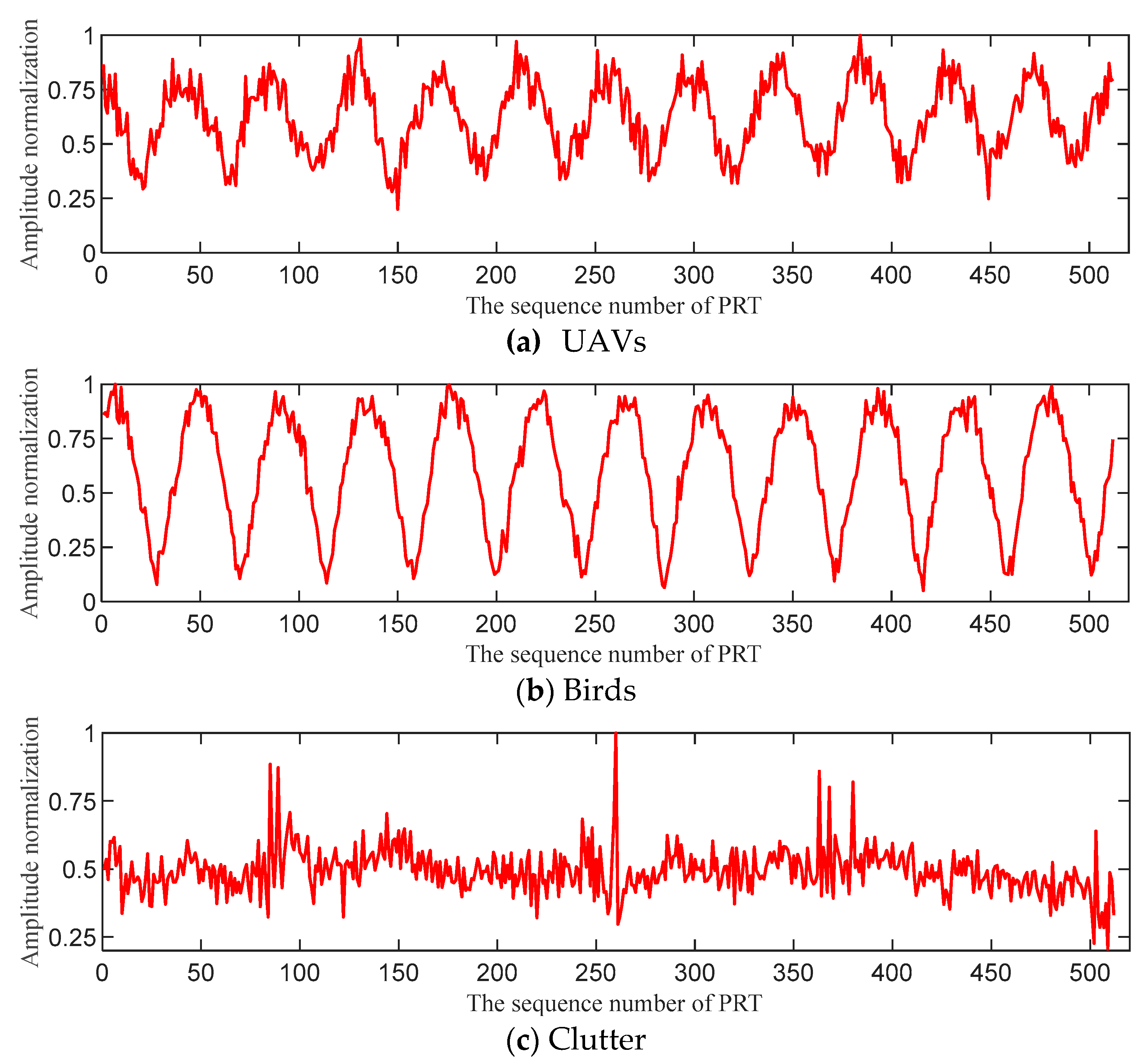
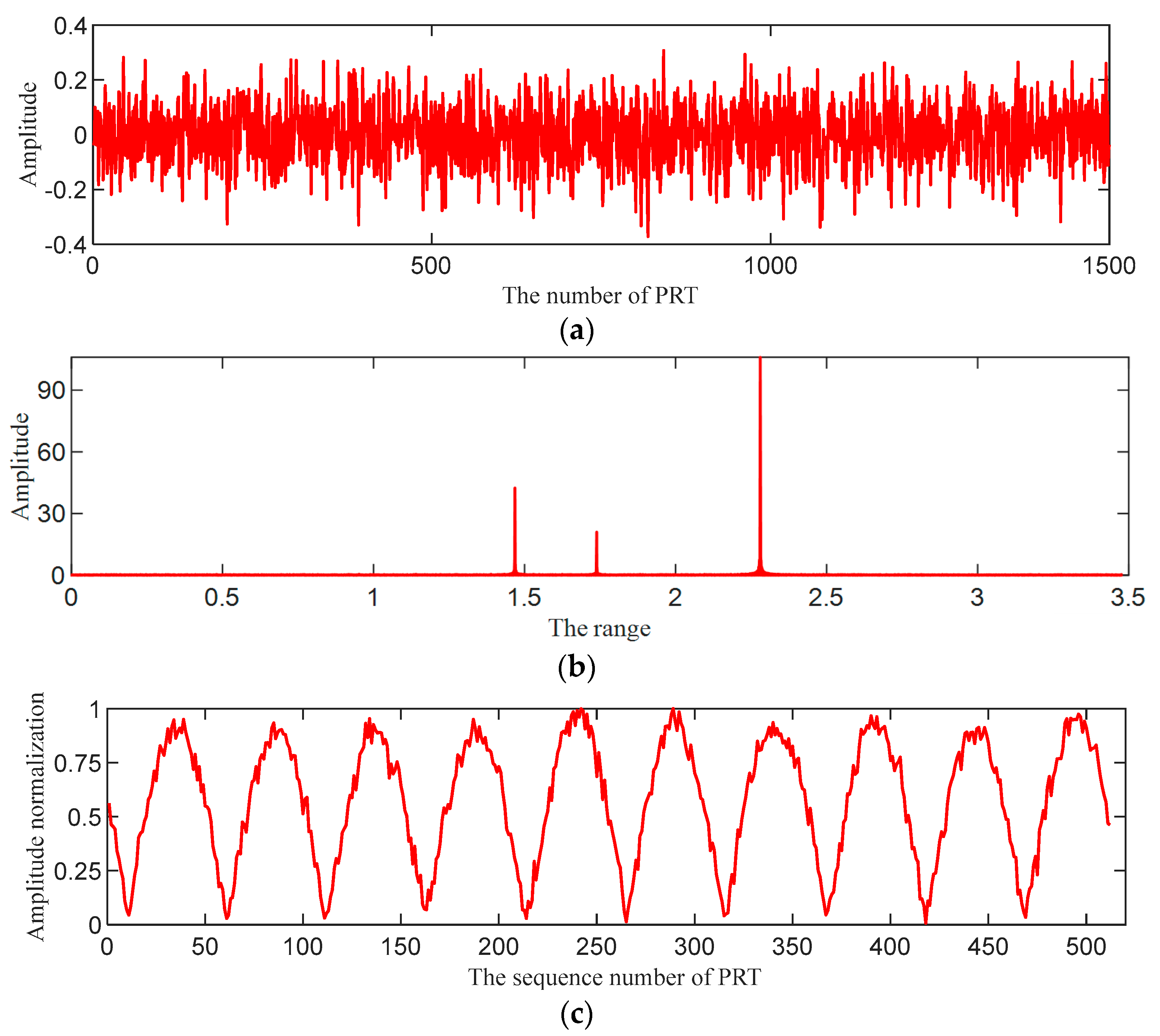
• An in-depth study of the motion frequency characteristics of birds, UAVs, and clutter targets in radar signals was conducted. The differences in frequencies within the radar signals show strong discriminability. By integrating the signal frequency difference characteristics of the targets with the network’s multi-frequency, multi-scale processing, an MFMSDC network was constructed, forming the core processing module of this paper.
• By flexibly using attention modules, the differences between targets and the background, especially in distinguishing clutter signals, were emphasized. This enabled the network to focus more on the features of birds and UAVs and effectively increased the network’s attention to the differentiated frequency characteristics of various targets, thereby improving the model’s performance.
• Through comparative experiments on the accumulation length of the slow-time dimension, it was determined that an accumulation length of 512 offers high timeliness for target classification. Method comparison experiments and ablation studies have demonstrated that directly processing one-dimensional radar signals in the slow-time dimension with a 1D-CNNs can efficiently distinguish categories of LSS targets.

2. Related Works

2.1. 1D-CNNs

1D-CNNs are specialized neural networks designed for processing time-series data, such as radar signals, where capturing temporal dynamics is crucial [19]. These networks leverage convolutional layers to automatically and adaptively learn spatial hierarchies of features from input data. 1D-CNNs have demonstrated effectiveness in various applications, including anomaly detection, environmental sensing, and particularly in radar signal processing for target detection and classification.

In recent years, deep learning has emerged as a pivotal technique across various domains including computer vision [20], speech recognition [21], and beyond, establishing itself as a cornerstone learning methodology. Its application in the individual identification of communication stations has garnered significant attention. While traditional methods like wavelet transform [22], Fourier transform [23], and Hilbert–Huang transform [24] are commonly employed to extract features from signals in the time, frequency, and time–frequency domains, they often overlook critical information during the extraction process, limiting the efficacy of feature characterization. Notably, ref. [25] introduces automated feature extraction and classification utilizing 1D-CNNs, yielding promising recognition outcomes. Additionally, ref. [26] demonstrates the direct learning of features from original vibration signals and fault diagnosis using 1D-CNNs. This underscores the broad applicability and efficacy of 1D-CNNs in one-dimensional signal classification tasks.

1D-CNNs offer a robust framework for handling the complex, noisy nature of radar data, enabling the extraction of meaningful features without the need for manual feature engineering [27]. Methods utilizing 1D-CNNs have been developed to address challenges in detecting and classifying LSS targets, improving signal-to-noise ratios, and reducing false positives. Recent academic research has advanced 1D-CNN applications in signal processing, offering robust methods for target recognition, anomaly detection, and signal classification. Techniques like multi-frequency multi-scale convolution and attention mechanisms have been introduced to improve feature extraction and network performance [28].

The research landscape in this domain continues to evolve, with ongoing exploration into the optimization of network architectures, enhancement of signal preprocessing techniques, and integration of attention mechanisms to improve model interpretability and performance [29,30]. Despite progress, challenges persist in dealing with highly dynamic target behaviors, cluttered environments, and adapting models to real-time processing requirements, indicating rich avenues for future research. In the field of one-dimensional signal processing research, current effective methodologies span traditional techniques such as Gaussian Naive Bayes (NB) [31] and Random Forest [32], complemented by deep learning-based one-dimensional networks like the Auto-Regressive Network (ARNet) [33], Resolution Adaptive Network (RANet) [34], and Residual Networks (ResNet) [35].

2.2. Radar Signal Processing

In the realm of radar signal processing, traditional methods have primarily focused on statistical and spectral analysis techniques, with notable contributions from scholars aiming to enhance detection and classification accuracy. Recently, one-dimensional CNNs have emerged as a powerful tool for processing radar signals, offering significant improvements in recognizing complex patterns within the data [36,37].

However, in the context of airport radar systems for UAVs and bird mitigation, current research has predominantly applied deep learning to extract features from the frequency and wavelet spectra of radar echoes. Studies by Kim B.K. [38] and Mendis G.J. [39], utilizing deep CNNs to analyze distinct micro-Doppler signatures of birds and UAVs, have demonstrated the potential for intelligent signal extraction and recognition. This is further exemplified by adaptations of CNN architectures for maritime micro-motion target classification.

In the realm of short-range radar systems, deep-learning-based one-dimensional signal processing remains an underexplored area. Due to characteristics, such as weight sharing and sparse connectivity, CNNs possess powerful feature extraction capabilities and generalizability, significantly enhancing the accuracy of target classification. They have now become an important solution for target classification in engineering applications. Researchers have ventured into this domain using various deep learning approaches for target recognition in high-resolution range profiles (HRRP) [40,41,42]. For the radar applications studied in this paper, many scholars employ a method using CNNs to process radar spectrograms by transforming the original echo signals from one-dimensional time series signals into two-dimensional image signals. These images are then inputted into CNNs for feature extraction and recognition classification. Jiang et al. [43] utilized a time–frequency analysis method based on windowed short-time Fourier transform to analyze the time–frequency characteristics of time-domain modulated signals. They applied a convolutional neural network based on transfer learning to classify modulation types according to RGB spectrogram images. Dongsuk Park et al. [44] proposed a deep-learning-based classification model that learns the micro-Doppler signatures (MDS) represented in the radar spectrogram images of targets. This research employs frequency modulated continuous wave (FMCW) radar to record various targets, including UAVs and human activities, converting these signals into spectrograms for the dataset. The ResNet-SP model, with a design based on ResNet-18 but requiring less computation, has demonstrated greater accuracy and stability, proving the potential of using deep learning for real-time UAV recognition.

All of the aforementioned methods require the conversion of one-dimensional signals into an image form for input, one which does not fully leverage the powerful feature extraction capabilities of CNNs and which still involves a certain degree of manual intervention [45]. Upon reviewing the literature, it has been found that there is limited research on the direct classification of birds and UAVs using deep learning convolutions on radar signals in one-dimensional space. However, one-dimensional convolution has already been widely applied in the processing of one-dimensional signals. Recent studies have made significant advances in the application of one-dimensional CNNs for radar signal processing, demonstrating progress in interference suppression, intelligent noise interference, and clutter suppression through deep learning techniques. Wang et al. [46] investigated an innovative interference suppression method that utilizes echo pre-processing for spread spectrum smearing (SMSP) interference, commonly employed in electronic countermeasures. This approach is designed to counteract the challenges associated with the suppression of SMSP interference without losing the energy of real targets, in turn achieving a 100% target detection probability under certain conditions. Zhu et al. [47] explored self-defense intelligent noise jamming, examining two typical intelligent noise barrier methods and proposing a suppression technique based on pulse frequency stepping. This method effectively filters radar echoes by exploiting the phase shifts caused by frequency stepping, thereby mitigating the threat posed by intelligent noise jamming. Additionally, Zou et al. [48] have devised a novel approach to airborne radar space-time adaptive processing (STAP), integrating sparse recovery (SR) with CNNs to overcome the limitations of conventional subscription methods. This hybrid approach, informed by deep unfolding, enhances the estimation accuracy of the spatiotemporal spectrum of clutter, thereby improving clutter suppression performance while simultaneously reducing computational complexity.

Previous approaches to spectrogram conversion have not only resulted in significant computational costs but also overlooked characteristics such as the target’s own motion frequency, relying solely on differences in image information. This presents challenges to the spectrogram conversion method. These advancements illustrate the potent application of 1D-CNNs in radar signal processing, offering promising solutions to longstanding challenges through the integration of deep learning algorithms. We conducted feature analysis on UAVs, birds, and clutter targets from the slow-time dimension and performed classification experiments using a one-dimensional convolutional network. It was found that this approach has a comparable classification capability to that of transforming signals into spectrograms, but with a significantly reduced computational load. Additionally, the frequency characteristics of UAVs, birds, and clutter targets exhibit considerable regularity and distinctiveness. The algorithm presented in this paper extracts multi-scale frequency features of targets through a network-embedded multi-frequency, multi-scale module, and incorporates an attention mechanism by which to enhance the network’s spatial and channel associations. This effectively increases the network’s focus on the differentiated frequency features of various targets, thereby providing stronger feature extraction capabilities than other algorithms.

3. Our Method

In this section, we explore the detailed application of the proposed CNN network for the identification of birds and UAVs, utilizing radar detection of slow-time dimension signals. Initially, a multi-frequency multi-scale convolutional neural network is constructed, leveraging the periodic characteristics of radar slow-time signals [49,50,51]. In the network design for recognition, the network features MFMSDC layers and transition layers. The MFMSDC layer employs varying stride lengths in the multi-scale convolution process for analyzing multiple frequencies, thus extracting multi-scale features of slow-time signals across different frequencies. The transition layers utilize attention modules to weight and filter the extracted features based on their significance.

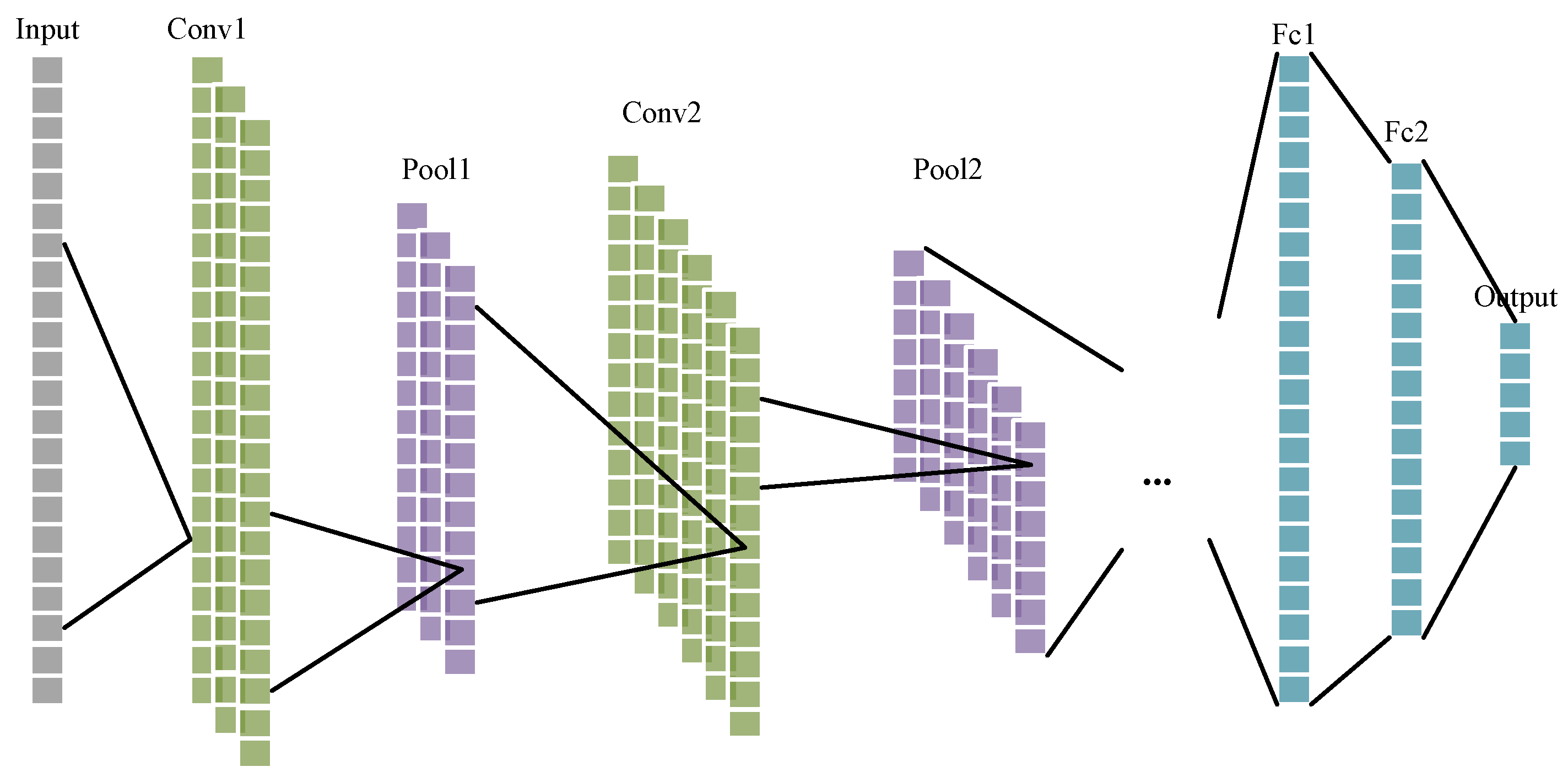
3.1. One-Dimensional Convolutional Neural Network

As depicted in Figure 2, the 1D-CNNs primarily utilize alternating stacks of convolutional layers and pooling layers to extract features from the input samples layer by layer. This process is followed by the application of fully connected layers that integrate and classify the extracted features, culminating in the identification of the radar slow-time dimension signal’s category.

The essence of the neural network training process lies in the model’s ability to learn the differences in data distributions. If there is a significant variance in the distribution of each batch of training samples, the network must adapt to these differences in every iteration, potentially slowing down the training process. A large discrepancy between the distributions of the training and test sets can diminish the network’s generalization ability. Moreover, during back-propagation, the network may experience vanishing gradients as the number of iterations increases. Therefore, batch normalization (BN) is employed to optimize the prediction model by alleviating the vanishing gradient issue in deep networks, accelerating model convergence, and reducing training time. The formula for BN is as follows:

$$y=\frac{\gamma }{\sqrt{Var\left[x\right]+\epsilon }}•x+\beta -\frac{\gamma E\left[x\right]}{\sqrt{Var\left[x\right]+\epsilon }}$$

(1)

where $E\left[x\right]$ and $Var\left[x\right]$ represent the unbiased estimates of the mean and variance of all batch features during the training phase, respectively. $\epsilon$ is a small positive number added to prevent division by zero, and learnable parameters $\gamma$ and $\beta$ are introduced. The purpose is to allow batch data to undergo scale transformation and shifting, enabling the restoration of the original data distribution through these adjustable parameters.

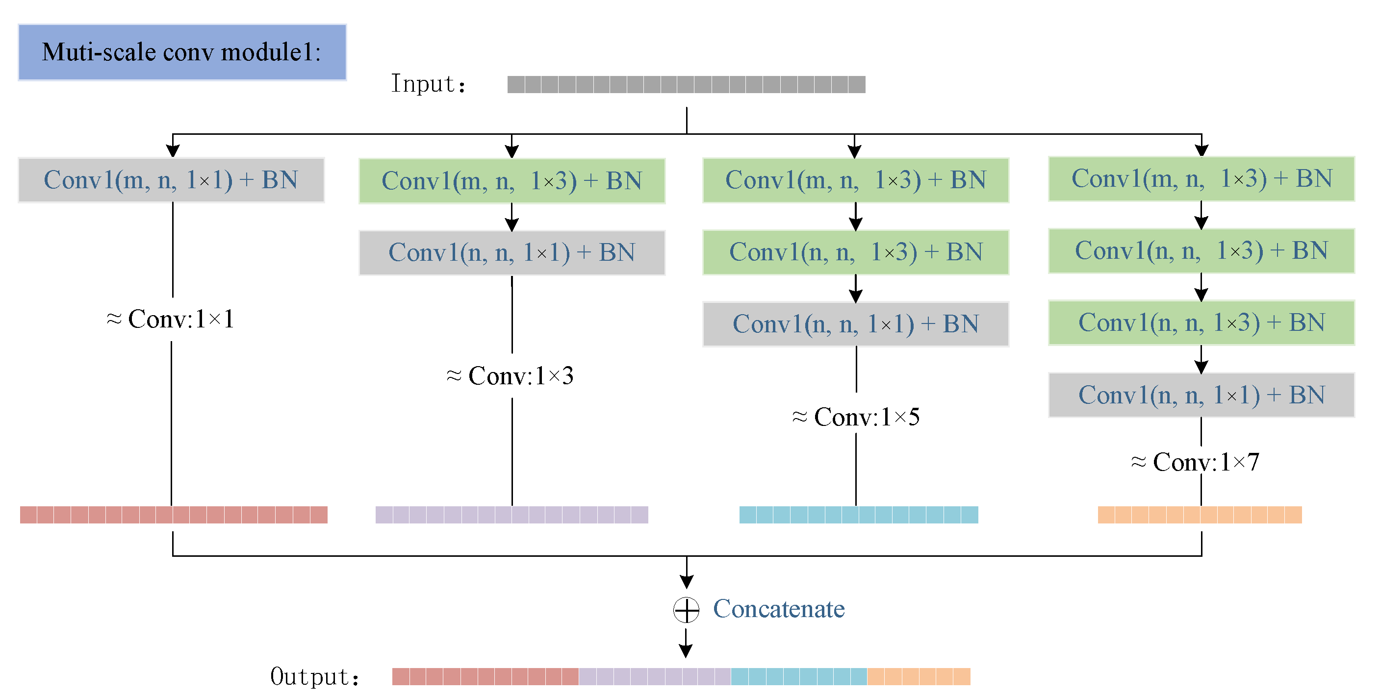
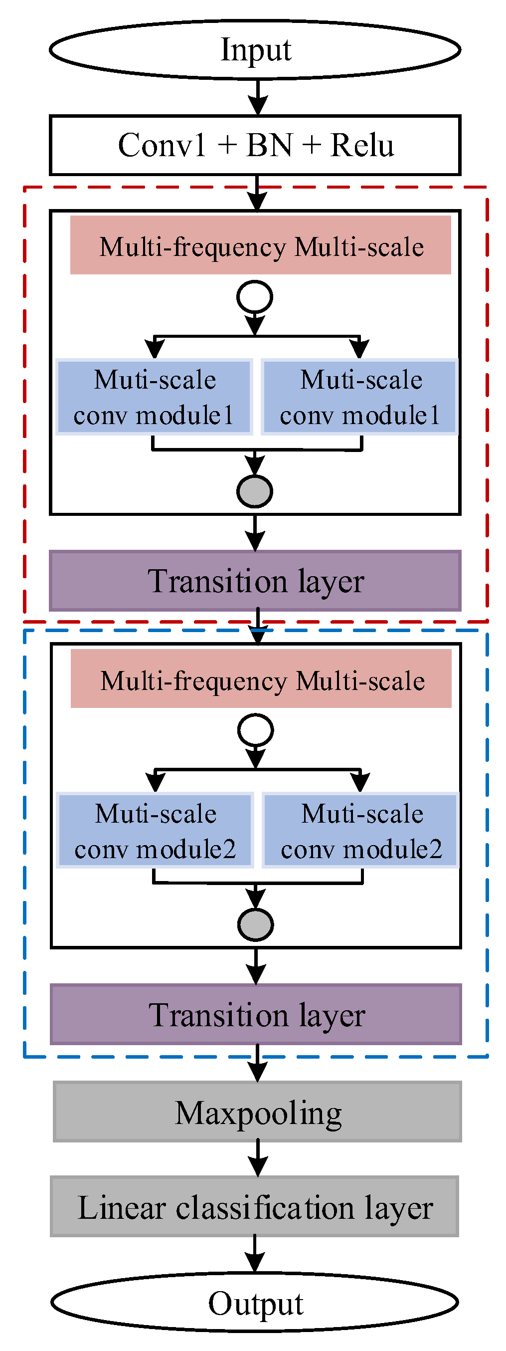
3.2. Multi-Frequency Multi-Scale Convolutional Neural Network

In this study, we elaborate on the use of slow-time dimension signals for the classification and identification of LSS radar targets. The LSS targets are diverse in nature and exhibit varying frequencies in the slow-time dimension signals. For instance, birds typically show low-frequency characteristics in these signals, whereas UAVs primarily exhibit higher harmonic frequencies. Hence, frequency serves as a crucial basis for identification and classification. To fully leverage the frequency information within the slow-time dimension signals, this study designs MFMSDC layers within the network based on the periodic characteristics of radar slow-time signals. As illustrated in Figure 3, the network comprises MFMSDC layers and transition layers. The MFMSDC layer employs varying stride lengths for multi-frequency analysis in order to extract multi-scale features across different frequencies of slow-time signals. In contrast, the transition layers use attention modules to weight and filter the extracted features based on their significance. The detailed architecture of both the MFMSDC layers and the transition layers will be further elaborated.

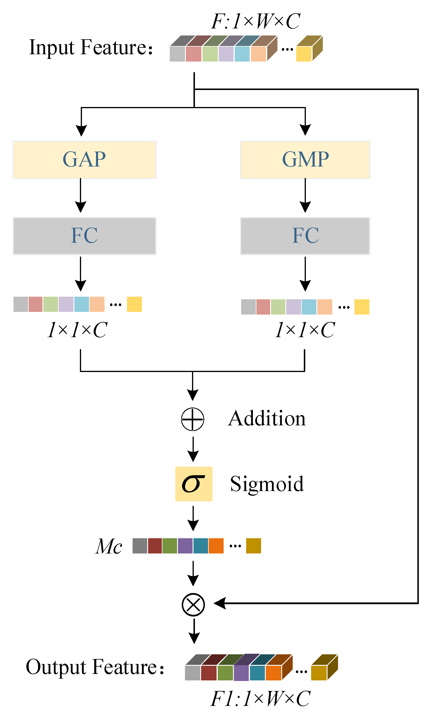
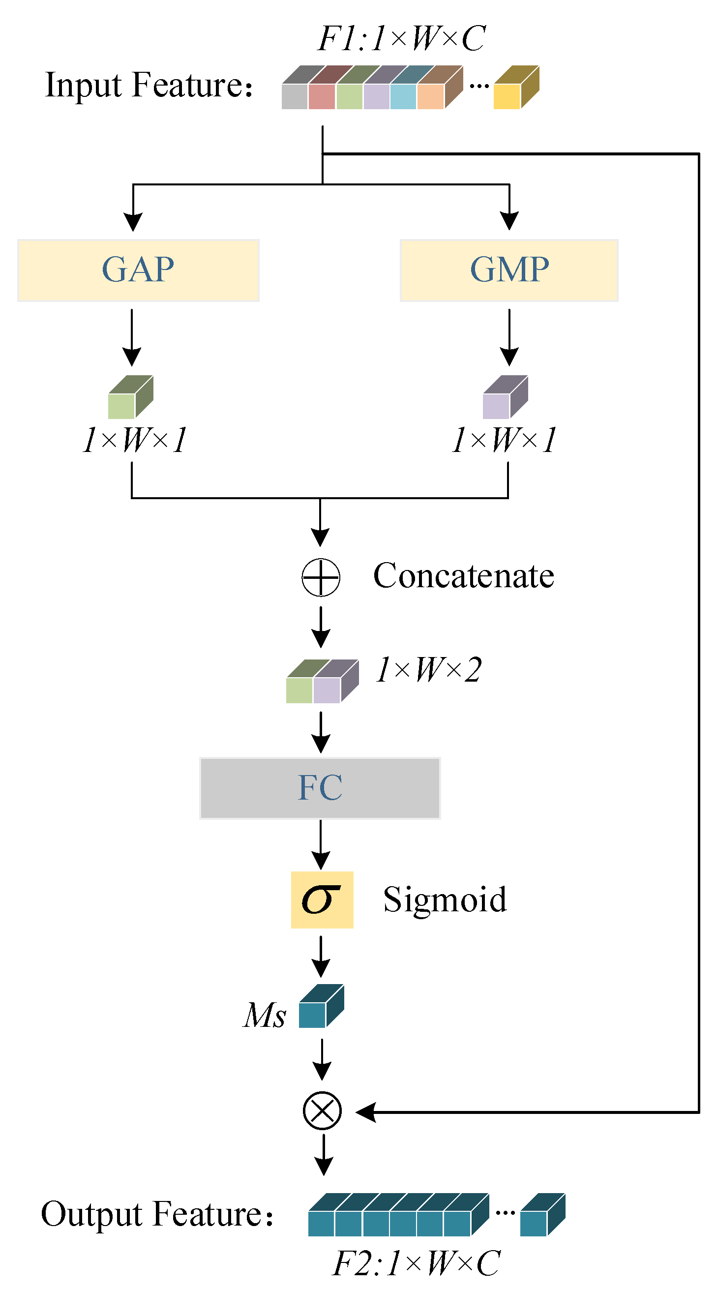
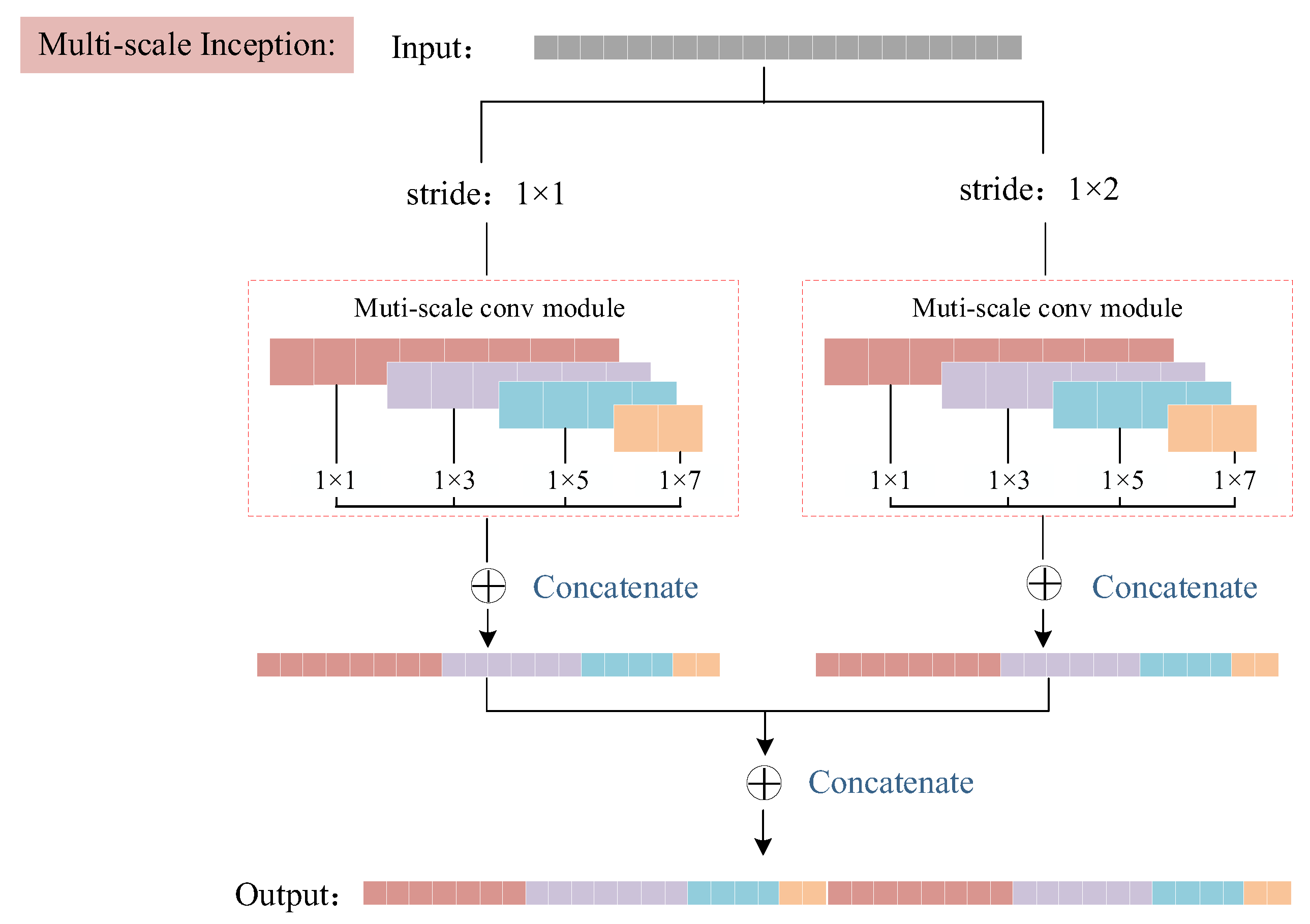
3.2.1. MFMSDC Module

The constructed network structure comprises two multi-frequency, multi-scale deformable convolution branches, one utilizing a convolution stride of 1 and the other employing a stride of 2, as depicted in Figure 4. Each branch incorporates four multi-scale convolution modules. This configuration facilitates the analysis of features across various frequencies of radar slow-time signals, with the stride-2 convolutions effectively down-sampling the slow-time signals to extract features from differing frequency bands.

The specific structure of the two multi-scale convolution modules nested within each multi-scale layer is depicted in Figure 5. It consists of four convolutional channels. The first channel processes input data with a 1 × 1 convolution and merges it directly with the data from other channels to preserve shallow feature characteristics. The subsequent three channels achieve convolutions of 1 × 3, 1 × 5, and 1 × 7, facilitated by stacking 1 × 3 convolutions, enabling multi-scale feature extraction from the input data. Each channel concludes with a 1 × 1 convolution to standardize the output dimensions across all channels. This is followed by the concatenation of data from the four channels to integrate multi-scale features.

In the structure depicted in Figure 5, each channel incorporates a 1 × 1 convolution operation. This operation is instrumental in reducing the number of feature channels, thereby decreasing the computational demand of the network. Additionally, it facilitates the integration of features across channels, enhancing the network’s capability to synthesize information from various sources for more effective analysis and interpretation.

Assuming the input to the MFMSDC layer is $x_0$, $x_0$ is fed into two multi-scale convolution modules. Each module has four channels extracting feature maps of different scales. The feature maps from all channels are then concatenated and fused, which can be represented by the following formula:

$$y=H(H({[x0•x1•x2•x3]}_{k=1})•H({[x0•x1•x2•x3]}_{k=2}))$$

(2)

In the formula, $•$ denotes the concatenation operation of feature vectors across channels, $[x0•x1•x2•x3]$ represents the concatenated feature vectors extracted by each channel of the multi-scale convolution module, $k$ is the stride, and $H(·)$ signifies a nonlinear transformation.

3.2.2. Transition Layer

While the multi-scale deformable convolution module captures multi-scale features of data, not all features equally contribute to the classification decisions. The attention modules can dynamically allocate weights based on the characteristics of input data, enabling the network to focus more on functions critical to the task. By dynamically adjusting the weights of features, attention modules can highlight the differences between targets and the background. For instance, UAVs in radar slow-time signals are characterized by periodicity and regularity, unlike clutter, which lacks these features. By flexibly employing attention mechanisms, the network pays more attention to the characteristics of UAV targets in radar slow-time signals, thus enhancing the effectiveness of target classification. Therefore, the use of attention modules can effectively increase the network’s focus on the differentiated frequency characteristics of various targets, thereby improving model performance. To emphasize crucial features, this study integrates a transition layer after each deformable convolution module, employing an attention mechanism for feature significance filtering. The structure is depicted in Figure 6. This mechanism adaptively weights multi-scale features, enhancing focus on essential attributes while disregarding irrelevant attributes. After feature extraction, attention modules compute weights in both the channel and the spatial dimensions, as depicted in the subsequent figure. This approach incorporates channel attention modules (CAM) and spatial attention modules (SAM), independently assessing and filtering the multi-scale features from both channel and spatial perspectives.

(a)

Channel Attention Module

As illustrated in Figure 7, the channel attention module takes an input feature vector F with dimensions 1 × W × C, and performs global max pooling (GMP) and global average pooling (GAP) based on width and height, resulting in two 1 × 1 × C feature vectors. These vectors are then passed through a one-dimensional convolution layer to produce two vectors of the same dimensions. By element-wise addition of these vectors and by applying a sigmoid activation function, the final channel attention weights M_C are generated. Finally, the input feature F is multiplied by M_C to output the channel-weighted feature F1.

(b)

The Spatial Attention Module

As shown in Figure 8, the spatial attention module uses the feature F1 output from the channel attention module as its input. It performs global max pooling and global average pooling across channels on the input feature vector, yielding two feature vectors of dimensions 1 × W × 1. These vectors are concatenated along the channel dimension to form a 1 × W × 2 dimensional feature vector. This vector is then subjected to a one-dimensional convolution to reduce it to a single-channel feature vector. A sigmoid activation function generates the spatial attention weights M_S, which are then multiplied with the input F1 to produce the spatially weighted feature F2.

(c)

The Linear Classification (LC) layer

Traditional CNNs often route extracted feature vectors through two or more fully connected layers before applying a softmax function to calculate the probability of each class for a sample, selecting the class with the highest probability as the sample’s category. However, the extensive parameters required for multiple fully connected layers, such as those for a feature map of dimensions W × H × C that is fed into a layer with M neurons and necessitating W × H × C × M parameters, can lead to increased computational complexity, slower processing speeds, more complicated parameter updates, lower efficiency, and potentially overfitting.

This study opts for global average pooling instead of fully connected layers for classification post-convolution. After several convolutions, it produces feature maps equal in number to the classes (W × H × Label), where “Label” denotes class count. Averaging each map yields a 1 × 1 × Label matrix, simplifying to a vector for classification. Global pooling, including both GAP and GMP, enhances training efficiency, parameter tuning, overfitting prevention, and spatial information aggregation, offering robustness against spatial transformations.

4. Experiment and Result Analysis

In this section, we begin by comparing the proposed multi-frequency multi-scale radar signal weak target detection network, which is constructed based on frequency periodicity features, to demonstrate its superior performance. Subsequent ablation studies are conducted to ascertain the efficacy of each component and the various configurations within our methodology. Finally, we discuss implementation details, offering insights into the practical application and optimization of the network for enhancing weak target detection capabilities in radar signal processing.

4.1. Evaluation Dataset

The data collection equipment utilized in this study is an LSS radar detection system, employing a full-domain phased-array radar operating in the S-band with HH polarization. The PRT is set at 115 microseconds, and the sampling rate is 20 MHz. The radar conducts target detection via electronic scanning. The original radar echoes captured at each wave position are subjected to pulse compression processing. For single-point data, an accumulation over 512 PRT yields the slow-time dimension data presented in this paper. All related data are verified through optoelectronic devices to confirm target information, ensuring the authenticity of the data used. The transformation from original echoes to the slow-time dimension signals described in this paper is visualized in Figure 9.

Figure 9 illustrates the schematic conversion from original echoes to slow-time dimension signals. Panel (a) presents a partial display of the amplitude–time distribution of the original echoes, where the row coordinate represents time, with the unit being milliseconds (ms), the echo collection is conducted at a sampling rate of 20 MHz and the column coordinate represents amplitude values. Panel (b) shows a partial display of the signal amplitude–distance distribution post-pulse compression, where the row coordinate denotes distance in kilometers and the column coordinate represents amplitude values. Panel (c) displays the distribution of amplitude normalization values over the accumulation number in the slow-time dimension. Here, the row coordinate represents 512 discrete PRT points and the vertical axis represents the normalized amplitude corresponding to each discrete PRT.

Additionally, through the integration of visual observation equipment for radar target validation, an LSS radar one-dimensional recognition database was established after an extensive three-month field collection and photoelectric verification process, as illustrated in

Table 1. The data collected in the field for UAVs and bird targets using a phased-array radar detection system.

Categories	Subcategories	Count
UAVs	UAV_10	222
	UAV_5	28
	UAV_4–6	469
	UAV_5–7	359
	UAV_1	68
	UAV_1–2	95
	UAV_2–3	127
birds	Bird_1–10	542
Clutter		2272
Total		4182

. The data encompasses three categories of target signals: UAVs, birds, and clutter. Each dataset has been manually verified to ensure the authenticity of the information. The collection of this data will facilitate the development of specialized radar system application technologies and provide a fundamental database for radar target identification.

In Table 1, “UAV_10” indicates signals detected by radar from UAVs at a distance of 10 km(kilometers), “UAV_5” signifies UAV signals detected at 5 km, “UAV_4–6” refers to UAVs hovering within 4 to 6 km as detected by radar, “UAV_5–7” represents UAVs flying within 5 to 7 km detected by radar, “UAV_1” marks UAV signals detected at 1 km, “UAV_1–2” shows UAVs hovering within 1 to 2 km detected by radar, “UAV_2–3” denotes UAVs flying within 2 to 3 km detected by radar, and “Bird_1–10” accounts for bird target signals detected by radar within 1 to 10 km.

The process involves preprocessing radar data in order to obtain the initial input data for the classification network proposed in this paper. Data preprocessing involves several steps, as follows: initially, collected data undergo cleansing; subsequently, the cleaned data is subjected to absolute amplitude detection using algorithms like Constant False Alarm Rate (CFAR), with detected target regions being clipped to a length of L. Then, the amplitude of the clipped data is calculated and normalized. Finally, the data are annotated with categories and divided into datasets, primarily into training, validation, and test sets, to facilitate structured analysis and model training.

(a)

Data cleansing for collected data primarily involves removing invalid, duplicate, and outlier entries from the database to ensure the integrity and reliability of the dataset for further processing and analysis.

(b)

Following data cleansing, absolute amplitude detection is carried out using algorithms such as CFAR. Based on the detection outcomes, data segments are extracted with a length of L, where L is determined by specific requirements and typically ranges from 256, 512, etc., with this study selecting 512 for extraction length.

(c)

For the data segments obtained after clipping, amplitude information is calculated. Assuming a point in the complex signal of length L is a + bi, the amplitude is calculated as follows:

$$z=\sqrt{a^2+b^2}$$

(3)

After calculating the amplitude, the signal can be represented as Z_i, where $i=1,2,\dots ,L$ denotes the index. The normalization of the amplitude-calculated signal X_i is then performed according to the following formula:

$$X_i=\frac{Z_i}{max(Z_i)}$$

(4)

In the formula, $i=1,2,\dots ,L$.

4.2. Implementation Details

Our experiments were implemented in Python using PyTorch (2.2.0). All experiments were conducted on a cluster equipped with 2 NVIDIA 3090 Tensor Core GPUs, facilitating high-performance computation for deep learning. The organized data were partitioned into training, validation, and test sets. The dataset comprised three categories, each containing 600 samples, for a total of 1800 samples. We randomly selected 360 samples from each category, totaling 1080, to form the training set. Additionally, 120 samples from each category, totaling 360, were allocated for the validation set, and the remaining 120 samples per category, also totaling 360, constituted the test set. These datasets do not overlap to ensure the authenticity of the algorithm testing results. To maximize GPU memory usage and rapidly reach the convergence point, we set the batch size to 128. The learning rate was set to 0.0005, with the learning rate decay set to 1/20 every 30,000 iterations. The dataset underwent a total of 150,000 iterations using stochastic gradient descent (SGD) with momentum optimizers.

4.3. Result Comparisons on Varying Length of Accumulation Time

In this paper, we compare the effects of our method based on features at four different accumulation time lengths: 128, 256, 512 and 1024. The selection of these lengths is motivated by several considerations: (1) FFT processing is particularly efficient for lengths that are powers of 2; (2) too short an accumulation time may result in the loss of target feature information; and (3) conversely, excessively long accumulation times can introduce redundant information and unnecessarily increase the number of parameters. Therefore, choosing an effective sequence length is crucial when accurately distinguishing between UAVs, birds, and clutter. Utilizing the MFMSDC developed in this study, we conducted signal recognition using the same target dataset across the four specified accumulation time lengths. The results of this analysis are presented in

Table 2. Experimental evaluation of the proposed method for target signals across four different accumulation time lengths, based on accuracy (A), precision (P), recall (R), and F1 score. The table presents the performance evaluation metrics for each accumulation time length. In the table, numbers in bold indicate the highest values in each column.

Length	Accuracy (A)	Precision (P)	Recall (R)	F1-Score
128	0.585	0.252	0.223	0.237
256	0.782	0.496	0.438	0.416
512	0.912	0.68	0.746	0.711
1024	0.913	0.65	0.756	0.704

.

As illustrated in Table 2, classification experiments were conducted on the datasets collected for UAVs, birds, and clutter using the one-dimensional network established in this study, across four different accumulation times: 128, 256, 512 and 1024. The results indicate that, compared with 128 and 256, all metrics show significant improvements at 512. While the classification outcomes at 1024 demonstrate a 0.001 increase in accuracy rate, other metrics experience a decline. Moreover, the data volume at 1024 is doubled compared with that at 512. Upon comprehensive analysis, an accumulation time of 512 proves to be the most cost-effective for target classification within this study. Consequently, subsequent experiments in this paper will be conducted based on 512 slow-time dimension accumulations for further experimental validation.

4.4. Result Comparisons on Self-Collected Dataset

Due to the scarcity of publicly available radar datasets, this study utilizes a self-collected dataset, comparing traditional methods (Gaussian NB, Random Forest) and deep learning-based one-dimensional networks (ARNet, RANet, ResNet18, ResNet34, ResNet50) as control groups for signal recognition. This comparison aims to validate the superiority of the proposed one-dimensional convolutional neural network in processing slow-time dimension signals. Experimental results are presented in

Table 3. Comparison of results on the self-collected dataset across different one-dimensional signal processing methods based on accuracy (A), precision (P), recall (R), and F1-score, demonstrating the performance evaluation metrics for each technique. In the table, numbers in bold indicate the highest values in each column.

Methods	Accuracy (A)	Precision (P)	Recall (R)	F1-Score
Gaussian NB	0.687	0.426	0.417	0.421
Random Forest	0.664	0.408	0.442	0.424
ARNet	0.785	0.452	0.423	0.437
RANet	0.732	0.456	0.418	0.436
Resnet18	0.811	0.488	0.413	0.447
Resnet34	0.833	0.485	0.426	0.454
Resnet50	0.845	0.51	0.582	0.527
Our	0.912	0.68	0.746	0.711

, where “Our” represents results after network refinement and data balancing.

From the experimental results depicted in Table 3, our method exhibits an approximate 23.6% improvement in average accuracy over traditional machine learning approaches, with moderate precision, and with F1 scores of 31.6% and 28.8%. Compared with methods employing one-dimensional neural networks (such as ARNet, RANet, ResNet18, ResNet34, and ResNet50), our approach demonstrates superior feature extraction capabilities by incorporating the motion characteristics of targets. This leads to the best performance across all relevant metrics.

4.5. Result Comparisons on Spectrogram

In the field of radar signal processing for LSS target classification and recognition, most approaches convert one-dimensional signals into spectrograms for subsequent image-based classification. To generate spectrograms, the radar signal is typically divided into short segments, and the Fourier transform is applied to each segment to obtain its frequency components. These frequency components are then plotted over time, resulting in a spectrogram in which the intensity of the plot corresponds with the magnitude of the frequency components.

By analyzing spectrograms, researchers can identify distinct patterns and signatures associated with different types of targets or phenomena. This approach enables efficient classification and recognition of targets in radar applications, especially for LSS targets where traditional methods may face challenges.

In our study, we leverage spectrogram processing techniques to transform one-dimensional radar signals into visual representations, allowing us to apply image-based classification methods, such as ResNet34 and ResNet50. This approach enhances our ability to accurately classify targets like birds, UAVs, and clutter, as depicted in Figure 10. Each row in the image represents an example of the display of spectrograms after classification using the method described in this paper.

Additionally, a quantitative comparison of the data classification results with the methods discussed in this manuscript was conducted, with experiments run on servers under identical configurations for a performance test comparison.

Table 4. Comparison of results between different two-dimensional ResNet networks on processed spectrogram results and the method described in this paper based on accuracy (A), precision (P), recall (R), and F1-score. In the table, numbers in bold indicate the highest values in each column.

Methods	Accuracy (A)	Precision (P)	Recall (R)
ResNet18	0.659	0.43	0.580
ResNet34	0.678	0.48	0.612
ResNet50	0.815	0.61	0.682
Our	0.912	0.68	0.746

presents the classification results of the two-dimensional networks ResNet18, ResNet34, and ResNet50 on spectrograms, comparing them with our method in terms of accuracy (A), precision (P), and recall (R). The detection effectiveness of our method significantly surpasses that of current and typical image processing-based classification techniques. Moreover, processing one-dimensional signal data requires considerably less data volume than two-dimensional spectrogram analysis, substantially enhancing the timeliness of radar signal processing.

4.6. Ablation Study

Ablation studies were conducted on self-collected data in order to assess the effectiveness of the designed MFMSDC network and optimized transition layers in enhancing method performance. The studies, based on the network depicted in Figure 2, involved variations like MFMSDC, CAM, SAM and LC layer. The first row corresponds to the standard one-dimensional convolutional network illustrated in Figure 2. MFMSDC1 denotes the network module on the left half of Figure 4 with a stride of 1, while MFMSDC2 represents the network module on the right half of Figure 4 with a stride of 2. MFMSDC3 refers to the multi-frequency network module in Figure 4, which combines both stride 1 and stride 2 configurations. The final row depicts the network structure designed in this study, which achieved optimal performance on relevant metrics. Through ablation experiments, as shown in

Table 5. Ablation study on the self-collected dataset, comparing the results from accuracy (A), precision (P), recall (R), and F1-score. In the table, numbers in bold indicate the highest values in each column, ‘’ indicates that the processing structure is not included during the network processing, while ‘ ’ indicates that the processing structure is included during the network processing.

MFMSDC1	MFMSDC2	MFMSDC3	CAM	SAM	LC	Accuracy (A)	Precision (P)	Recall (R)	F1-Score
						0.456	0.34	0.385	0.400
						0.602	0.39	0.420	0.450
						0.651	0.45	0.481	0.508
						0.851	0.51	0.612	0.556
						0.871	0.57	0.672	0.617
						0.898	0.53	0.712	0.608
						0.912	0.68	0.746	0.711

, the impact of each module on the overall network performance is demonstrated.

Table 5 demonstrates that incorporating multi-frequency multi-scale deformable convolution, channel and spatial attention mechanisms, and an LC layer significantly enhances model performance, enabling the prediction of a greater number of positive samples. It is also evident that incorporating the motion frequency information of the targets significantly enhances the classification performance for the subjects of this study, namely birds and UAVs.

4.6.1. The Impact of the MFMSDC Module

The manuscript discusses the construction of a network architecture with MFMSDC convolution layers, which utilize convolutions of two different strides in order to analyze features across various frequencies of radar slow-time signals. Specifically, the stride-2 convolution allows for multiple down-sampling of slow-time signals, facilitating the extraction of features from signals of diverse frequencies. By simultaneously capitalizing on the extraction and utilization of the low-frequency features of bird targets and high-frequency characteristics of UAVs, the study fully leverages the frequency information embedded in the slow-time dimension signals. This approach enhances the network’s capability to extract frequency multi-scale features of slow-time signals, significantly bolstering the network’s robustness. Table 5 reveals that MFMSDC3, which considers multi-frequency feature information, when compared with the low-frequency feature extraction method of MFMSDC1, results in an in increase in accuracy of 24.9%, precision of 12.0%, recall of 19.2%, and F1 score of 10.6%. Furthermore, when comparing MFMSDC3, which considers multi-frequency feature information, with the high-frequency feature extraction method of MFMSDC2, accuracy increased by 20.0%, precision by 6.0%, recall by 13.1%, and the F1 score by 4.8%.

4.6.2. The Impact of Optimizing the Transition Layer

The integration of attention mechanisms following each multi-scale deformable convolution module significantly enhances model performance by focusing on essential features. This approach enables the adaptive weighting of multi-scale features, improving the neural network’s attention to critical attributes while disregarding irrelevant ones. Implementing this attention structure has notably improved various model metrics, boosting the recall rate in particular, by 10%. This improvement underscores the effectiveness of attention mechanisms in optimizing feature selection for better classification outcomes.

Opting for GAP instead of fully connected layers for post-convolution classification brings significant advantages. GAP reduces training time due to the absence of parameters, eliminating the need for adjustments to the optimization algorithm and effectively preventing overfitting. Additionally, by aggregating spatial information, GAP enhances the model’s robustness to spatial transformations, providing a streamlined and efficient method for feature extraction and classification.

Building on the experiments in Section 4.6.1, the network structure was refined by incorporating attention modules within the transition layers, enhancing feature connectivity both channel-wise and spatially. This modification allows the model to focus on more critical features from a vast dataset while employing linear operations in the classification layer to effectively prevent overfitting. Consequently, there was a noticeable improvement in all evaluation metrics of the network.

The enhancements made to the one-dimensional convolutional neural network structure, as detailed in Table 5, resulted in significant performance improvements compared with a standard one-dimensional convolutional network, accuracy increased by 45.6%, precision by 34%, recall by 36.1%, and the F1 score by 31.1%. The outcomes of these improvements are illustrated in Figure 11.

5. Conclusions

In this paper, we have introduced a novel approach to radar echo recognition that leverages a 1D-CNN to directly extract features from the slow-time dimension of radar signals. This methodology marks a departure from conventional techniques that rely heavily on the transformation of signals into the frequency or wavelet domains for feature extraction. By directly analyzing the slow-time dimension, our approach simplifies the processing workflow and enhances the efficiency of feature extraction.

The core of our network architecture is the MFMSDC layers, which facilitate the extraction of features across a broad spectrum of signal frequencies. Furthermore, the integration of attention modules within the transition layers of the network significantly improves feature connectivity, both channel-wise and spatially, thereby bolstering the network’s capacity to focus on pertinent features while minimizing the influence of irrelevant data. Crucially, the implementation of linear operations in the classification layer of our network serves to mitigate the risk of overfitting, thereby ensuring more reliable and generalizable classification outcomes. Ablation studies conducted as part of our research validate the effectiveness of our network design, demonstrating notable improvements across all evaluation metrics when compared with existing classification networks.

The findings of our study underscore the potential of employing 1D-CNNs for the recognition of radar echoes, specifically in the context of LSS target detection. Our method not only streamlines the analytic process but also achieves superior classification performance, thereby offering a promising avenue for future research and development in radar signal processing.

References

1. Chen, W.H.; Liu, J.; Chen, X.L. Non-cooperative UAV Target Recognition in Low-altitude Airspace Based on Motion Model. J. Beijing Univ. Aeronaut. Astronaut. 2019, 45, 687–694. [Google Scholar] [CrossRef]
2. Wu, X.S.; Fang, Z.J.; Chen, T.H. Research on Civil UAV Countermeasure Technology. China Radio 2018, 3, 55–58. [Google Scholar] [CrossRef]
3. Han, Y.; Liu, H.; Wang, Y.; Liu, C. A comprehensive review for typical applications based upon unmanned aerial vehicle platform. IEEE J. Sel. Top. Appl. Earth Obs. Remote Sens. 2022, 15, 9654–9666. [Google Scholar] [CrossRef]
4. Han, Y.; Deng, C.; Zhao, B.; Tao, D. State-aware anti-drift object tracking. IEEE Trans. Image Process. 2019, 28, 4075–4086. [Google Scholar] [CrossRef] [PubMed]
5. Han, Y.; Deng, C.; Zhao, B.; Zhao, B. Spatial-temporal context-aware tracking. IEEE Signal Process. Lett. 2019, 26, 500–504. [Google Scholar] [CrossRef]
6. Deng, C.; He, S.; Han, Y.; Zhao, B. Learning dynamic spatial-temporal regularization for UAV object tracking. IEEE Signal Process. Lett. 2021, 28, 1230–1234. [Google Scholar] [CrossRef]
7. Zhao, B.; Wang, H.; Tang, L.; Han, Y. Towards long–term UAV object tracking via effective feature matching. Electron. Lett. 2020, 56, 1056–1059. [Google Scholar] [CrossRef]
8. Han, Y.; Wang, H.; Zhang, Z.; Wang, Z. Boundary–aware vehicle tracking upon UAV. Electron. Lett. 2020, 56, 873–876. [Google Scholar] [CrossRef]
9. Luo, H.H.; Lu, Y.Q. Ability Status and Development Trend of Anti-“low, slow and small” UAVs. Aerodyn. Missile J. 2019, 6, 32–36. [Google Scholar] [CrossRef]
10. Chen, W.H.; Li, J. Review on Development and Applications of Avian Radar Technology. Mod. Radar 2017, 39, 7–17. [Google Scholar] [CrossRef]
11. Chen, X.L.; Guan, J.; Huang, Y. Radar Low-observable Target Detection. Sci. Technol. Rev. 2017, 35, 30–38. [Google Scholar] [CrossRef]
12. Wang, F.Y.; Guo, R.J.; Hao, M. Balloon Borne Radar Target Detection within Ground Clutter Based on Fractal Character. National Defense Invention Patent Application No.201110015890.X, 16 September 2011. [Google Scholar]
13. Wang, C.; Xia, H.Y.; Liu, Y.P. Spatial Resolution Enhancement of Coherent Doppler Wind Lidar Using Joint Time-frequency Analysis. Opt. Commun. 2018, 424, 48–53. [Google Scholar] [CrossRef]
14. Du, L.; Chen, X.Y.; Shi, Y. MMRGait-1.0: A Radar Time-frequency Spectrogram Dataset for Gait Recognition under Multi-view and Multi-wearing Conditions. J. Radars 2019, 45, 687–694. [Google Scholar] [CrossRef]
15. Hinton, G.E.; Osindero, S.; Teh, Y.W. A Fast Learning Algorithm for Deep Belief Nets. Neural Comput. 2006, 18, 1527–1554. [Google Scholar] [CrossRef] [PubMed]
16. Krizhevsky, A.; Sutskever, I.; Hinton, G.E. ImageNet Classification with Deep Convolutional Neural Networks. In Proceedings of the Advances in Neural Information Processing Systems, Lake Tahoe, NV, USA, 3–6 December 2012; Volume 1, pp. 1097–1105. [Google Scholar]
17. Kan, S.; He, Z.; Cen, Y.; Li, Y.; Mladenovic, V.; He, Z. Contrastive Bayesian Analysis for Deep Metric Learning. IEEE Trans. Pattern Anal. Mach. Intell. 2023, 45, 7220–7238. [Google Scholar] [CrossRef] [PubMed]
18. Yu, B.; Guo, Z.; Asian, S. Flight Delay Prediction for Commercial Air Transport: A Deep Learning Approach. Transp. Res. Part E Logist. Transp. Rev. 2019, 125, 203–221. [Google Scholar] [CrossRef]
19. Su, N.Y.; Chen, X.L.; Guan, J. Detection and Classification of Maritime Target with Micro Motion Based on CNNs. J. Radars 2018, 7, 565–574. [Google Scholar] [CrossRef]
20. Hinton, G.; Salakhutdinov, R. Reducing the Dimensionality of Data with Neural Networks. Science 2006, 313, 504–507. [Google Scholar] [CrossRef]
21. Hinton, G.; Deng, L.; Yu, D. Deep Neural Networks for Acoustic Modeling in Speech Recognition: The Shared Views of Four Research Groups. IEEE Signal Process. Mag. 2012, 29, 82–97. [Google Scholar] [CrossRef]
22. Yu, Q.; Cheng, W.; Li, J.W. Specific Emitter Identification Using Wavelet Transform Feature Extraction. Signal Process. 2018, 34, 1076–1085. [Google Scholar]
23. Ye, W.Q.; Yu, Z.F. Signal Recognition Method Based on Joint Time-frequency Radiation Source. Electron. Warf. Technol. 2018, 33, 16–19. [Google Scholar]
24. Wu, H.; Yuan, Y.; Wang, X. Specific Emitter Identification Based on Hilbert-Huang Transform-based-time Frequency-energy Distribution Features. IET Commun. 2014, 8, 2404–2412. [Google Scholar] [CrossRef]
25. Yang, Y.; Lian, J.J.; Zhou, G.G.; Chen, Z.H. Steel Truss Structure Damage Identification Based on One-dimensional Convolutional Neural Network. In Proceedings of the Tianjin University, Tianjin Steel Structure Society, Academic Committee of the National Symposium on Modern Structural Engineering, Tianjin, China, 19 September 2020; Volume 4. [Google Scholar]
26. Wu, C.Z.; Jiang, P.C.; Feng, F.Z.; Chen, T.; Chen, X.L. Gearbox Fault Diagnosis Based on One-dimensional Convolutional Neural Network. Vib. Shock 2018, 37, 51–56. [Google Scholar]
27. Li, G.; Zhang, R.; Ritchie, M. Sparsity-driven MicroDoppler Feature Extraction for Dynamic Hand Gesture Recognition. IEEE Trans. Aerosp. Electron. Syst. 2018, 54, 655–665. [Google Scholar] [CrossRef]
28. Tao, C.; Pan, H.B.; Li, Y.S. Unsupervised Spectral-spatial Feature Learning with Stacked Sparse Autoencoder for Hyperspectral Imagery Classification. IEEE Geosci. Remote Sens. Lett. 2015, 12, 2438–2442. [Google Scholar] [CrossRef]
29. Wang, Q.; Wu, B.; Zhu, P. Supplementary Material for ECA-Net: Efficient Channel Attention for Deep Convolutional Neural Networks. In Proceedings of the 2020 IEEE/CVF Conference on Computer Vision and Pattern Recognition, Seattle, WA, USA, 14–19 June 2020; pp. 13–19. [Google Scholar]
30. Deng, Y.J.; Wu, Z.H.; Lin, Y.F. Flight Passenger Load Factors Prediction Based on RNN Using Multi Granularity Time Attention. Comput. Eng. 2020, 46, 294–301. [Google Scholar]
31. Li, D.Q.; Hu, S.J.; He, W.P.; Zhou, B.Q. Correction to: The Area Prediction of Western North Pacific Subtropical High in Summer Based on Gaussian Naive Bayes. Clim. Dyn. 2022, 60, 4199–4205. [Google Scholar] [CrossRef]
32. Svetnik, V. Random Forest: A Classification and Regression Tool for Compound Classification and QSAR Modeling. J. Chem. Inf. Comput. Sci. 2003, 43, 1947–1958. [Google Scholar] [CrossRef] [PubMed]
33. Triebe, O.; Laptev, N.; Rajagopal, R. AR-Net: A Simple Auto-Regressive Neural Network for Time-series. arXiv 2019, arXiv:1911.12436. [Google Scholar]
34. Yang, L.; Han, Y.Z.; Chen, X. Resolution Adaptive Networks for Efficient Inference. In Proceedings of the Computer Vision and Pattern Recognition (CVPR), Seattle, WA, USA, 14–19 June 2020. [Google Scholar] [CrossRef]
35. He, K.M.; Zhang, X.Y.; Ren, S.Q. Deep Residual Learning for Image Recognition. In Proceedings of the IEEE Conference on Computer Vision and Pattern Recognition, Las Vegas, NV, USA, 27–30 June 2016; pp. 770–778. [Google Scholar]
36. Devlin, J.; Chang, M.W.; Lee, K. Bert: Pre-training of Deep Bidirectional Transformers for Language Understanding. In Proceedings of the 2019 Conference of the North American Chapter of the Association for Computational Linguistics, Human Language Technologies, Minneapolis, MN, USA, 2–7 June 2019; pp. 4171–4186. [Google Scholar] [CrossRef]
37. Gui, R.H.; Wang, W.Q.; Pan, Y. Cognitive Target Tracking Via Angle-range-Doppler Estimation with Transmit Subaperturing FDA Radar. IEEE J. Sel. Top. Signal Process. 2018, 12, 76–89. [Google Scholar] [CrossRef]
38. Kim, B.K.; Kang, H.S.; Park, S.O. Drone Classification Using Convolutional Neural Networks with Merged Doppler Images. IEEE Geosci. Remote Sens. Lett. 2017, 14, 38–42. [Google Scholar] [CrossRef]
39. Mendis, G.J.; Wei, J.; Madanayake, A. Deep Learning Cognitive Radar for Micro UAS Detection and Classification. In Proceedings of the 2017 Cognitive Communications for Aerospace Applications Workshop, Cleveland, OH, USA, 27–28 June 2017; pp. 1–5. [Google Scholar] [CrossRef]
40. Wang, Y.H.; Ma, Y.C.; Zhang, Z.L.; Zhang, X.; Zhang, L. Type-aspect Disentanglement Network for HRRP Target Recognition with Missing Aspects. IEEE Geosci. Remote Sens. Lett. 2023, 20, 350–930. [Google Scholar] [CrossRef]
41. Zhang, L.; Li, Y.; Wang, W.H.; Wang, J.F.; Long, T. Polarimetric HRRP Recognition Based on ConvLSTM with Self-Attention. IEEE Sens. J. 2021, 21, 7884–7898. [Google Scholar] [CrossRef]
42. Song, J.; Wang, Y.H.; Chen, W.; Li, Y.; Wang, J.F. Radar HRRP Recognition Based on CNN. J. Eng. 2019, 21, 7766–7769. [Google Scholar] [CrossRef]
43. Jiang, W.; Wu, X.; Wang, Y.; Chen, B.; Feng, W.; Jin, Y. Time–Frequency-Analysis-Based Blind Modulation Classification for Multiple-Antenna Systems. Sensors 2021, 21, 231. [Google Scholar] [CrossRef]
44. Park, D.; Lee, S.; Park, S.; Kwak, N. Radar-Spectrogram-Based UAV Classification Using Convolutional Neural Networks. Sensors 2021, 21, 210. [Google Scholar] [CrossRef] [PubMed]
45. Huang, C.-Y.; Dzulfikri, Z. Stamping Monitoring by Using an Adaptive 1D Convolutional Neural Network. Sensors 2021, 21, 262. [Google Scholar] [CrossRef] [PubMed]
46. Wang, X.; Chen, H.; Liu, W.; Zhang, L.; Li, B.; Ni, M. Echo Preprocessing-Based Smeared Spectrum Interference Suppression. Electronics 2023, 12, 3690. [Google Scholar] [CrossRef]
47. Zhu, Y.; Zhang, Z.; Li, B.; Zhou, B.; Chen, H.; Wang, Y. Analysis of Characteristics and Suppression Methods for Self-Defense Smart Noise Jamming. Electronics 2023, 12, 3270. [Google Scholar] [CrossRef]
48. Zou, B.; Feng, W.; Zhu, H. Airborne Radar STAP Method Based on Deep Unfolding and Convolutional Neural Networks. Electronics 2023, 12, 3140. [Google Scholar] [CrossRef]
49. Confuorto, P.; Di, M.D.; Centolanza, G. Postfailure Evolution Analysis of a Rainfall-triggered Landslide by Multi-temporal Interferometry SAR Approaches Integrated with Geotechnical Analysis. Remote Sens. Environ. 2017, 188, 51–72. [Google Scholar] [CrossRef]
50. Lundén, J.; Koivunen, V. Deep Learning for HRRP-based Target Recognition in Multistatic Radar Systems. In Proceedings of the 2016 IEEE Radar Conference, Philadelphia, PA, USA, 2–6 May 2016; pp. 1–6. [Google Scholar]
51. Liu, Y.; Long, T.; Zhang, L.; Wang, Y.; Zhang, X.; Li, Y. SDHC: Joint semantic-data guided hierarchical classification for fine-grained HRRP target recognition. IEEE Trans. Aerosp. Electron. Syst. 2024; early access. [Google Scholar] [CrossRef]
Figure 1. Schematic diagram of slow-time dimension signals for three types of targets. Each image displays the distribution of amplitude normalization values over the accumulation number in the slow-time dimension. Here, the row coordinate represents 512 discrete PRT points, and the vertical axis represents the normalized amplitude corresponding to each discrete PRT. (a) UAVs. (b) Birds. (c) Clutter.
Remotesensing 16 01431 g001
Figure 2. Structure diagram of a one-dimensional convolutional neural network.
Remotesensing 16 01431 g002
Figure 3. Overall structure diagram of the multi-frequency multi-scale convolutional network.
Remotesensing 16 01431 g003
Figure 4. Structure diagram of the MFMSDC module.
Remotesensing 16 01431 g004
Figure 5. Structure diagram of the multi-scale convolution module.
Remotesensing 16 01431 g005
Figure 6. Transition layer network structure.
Remotesensing 16 01431 g006
Figure 7. Channel attention module structure diagram.
Remotesensing 16 01431 g007
Figure 8. Spatial attention module structure diagram.
Remotesensing 16 01431 g008
Figure 9. Schematic of the conversion from original echoes to slow-time dimension signals. (a) A partial display of the amplitude-time distribution of the original echoes. (b) A partial display of the signal amplitude–distance distribution post-pulse compression. (c) The distribution of amplitude normalization values over the accumulation number of PRT in the slow-time dimension.
Remotesensing 16 01431 g009
Figure 10. The spectrogram recognition results, with each row representing a category of targets. The images illustrate examples of the spectrogram displays after classification using the method described in this paper.
Remotesensing 16 01431 g010
Figure 11. Display of typical target classification result data. Each image displays the distribution of amplitude normalization values over the number of accumulations in the slow-time dimension, following the accumulation of amplitude information. In these images, the row coordinate represents 512 discrete PRT points, and the vertical axis represents the normalized amplitude corresponding to each discrete PRT.
Remotesensing 16 01431 g011