Lake Ice Thickness Retrieval Method with ICESat-2-Assisted CyroSat-2 Echo Peak Selection

Abstract

Lake ice thickness (LIT) is one of the key climate variables in the lake ice domain, but there are currently large uncertainties in the retrieval of LIT. We present and validate a new LIT retrieval method that utilizes ICESat-2 data to assist CryoSat-2 echo peak selection, aiming to improve the accuracy of LIT retrieval and enable data acquisition without on-site measurements. The method involves screening out similar ICESat-2 and CryoSat-2 tracks based on time and space constraints. It also involves dynamically adjusting the range constraint window of CryoSat-2 waveforms based on the high-precision lake ice surface ellipsoid height obtained from ICESat-2/ATL06 data. Within this range constraint window, the peak selection strategy is used to determine the scattering interfaces between snow-ice and ice-water. By utilizing the distance between the scattering horizons, the thickness of the lake ice can be determined. We performed the ice thickness retrieval experiment for Baker Lake in winter and verified it against the on-site measurement data. The results showed that the accuracy was about 0.143 m. At the same time, we performed the ice thickness retrieval experiment for Great Bear Lake (GBL), which does not have on-site measurement data, and compared it with the climate change trend of GBL. The results showed that the retrieval results were consistent with the climate change trend of GBL, confirming the validity of the proposed method.

1. Introduction

Lake ice is an essential component of the climatic environment within the Arctic and sub-Arctic regions and is a critical research object in the cryosphere. In the middle- and high-latitude regions of the Northern Hemisphere, the maximum area covered by lake ice can reach $1.59\times {10}^6{ \mathrm{km}}^2$ as the climate cycles [1]. Lake ice thickness (LIT), an essential climate variable in the lake ice domain of the Global Climate Observing System [2], is effective in ensuring the safety of ice activities and providing data support for climate forecasting. In addition, LIT not only affects the ecology, climate, and environment of the Arctic and sub-Arctic regions but also significantly impacts the economic development of local societies [3,4,5]. With the onset of global warming, some lakes appear ice-free during the winter months [6]. Brown and Duguay predicted the LIT in the Arctic and sub-Arctic regions based on a lake ice model, and their results showed that the mean maximum ice thickness will decrease by 5–60 cm by 2070 [7]. In recent years, lake ice phenology records from artificial stations have decreased in number. According to the Global Lake and River Ice Phenology Database, an average of 970 observations per year were recorded in the Northern Hemisphere between 1970 and 1990, but only an average of 198 observations were made between 2004 and 2020 [8]. Remote sensing technology has become the most important tool for current observations in the middle- and high-latitude regions.

Remote sensing methods for LIT retrieval can be primarily categorized into three types based on the type of sensors used: thermal infrared remote sensing, passive microwave remote sensing, and active microwave remote sensing [9]. LIT retrieval based on the thermal infrared remote sensing simplifies and makes several assumptions regarding the physical processes of lake ice. The method based on the thermal infrared remote sensing primarily utilizes surface temperature information of the lake ice and combines it with corresponding models to estimate the ice thickness. The model parameters and performance may vary significantly in different regions [10]. The passive microwave remote sensing method has a low spatial resolution and can only perform ice thickness retrieval for lakes with large water areas. It relies on the measured or simulated LIT to construct a regression equation between the bright temperature and LIT, which cannot guarantee the robustness of the parameters transplanted to other lakes [11]. Active microwave remote sensing data can be divided into two categories; one is synthetic aperture radar (SAR) data and the other is radar altimetry data. LIT retrieval based on SAR images mainly utilizes the fitting relationship between the backward scattering coefficient and the LIT [12,13], but this method is limited by the special imaging regime of SAR, and the retrieval accuracy is relatively low when the thickness of the lake ice exceeds 40 cm [14]. And the most commonly used ice thickness retrieval data are radar altimetry data.

There are also two types of methods for LIT retrieval using radar altimetry data: one utilizes the backscattering coefficient of the altimetry radar, while the other is based on the analysis of the radar waveform. The main idea of the first method is that the ice layer absorbs and scatters effects on radar waves. As the ice thickness increases, the corresponding backscattering coefficient gradually decreases. Therefore, it is possible to establish a regression relationship between the radar backscattering and the ice thickness, thereby enabling an accurate ice thickness retrieval [3]. Li et al. [15] combined radar altimetry waveforms and backscattering coefficients to estimate the LIT, which utilized a logarithmic regression model to establish the relationship between the backscattering coefficient and ice thickness; the accuracy of estimating the LIT was approximately 0.2 m. However, recent studies have shown that the backscattering coefficient is mainly affected by the roughness of the lake ice surface, and an increase in the LIT does not have a significant effect on the backscattering coefficient of lake ice [8]; therefore, the use of the backscattering coefficient in LIT retrieval needs to be verified for the reasonableness of the model. The thickness retrieval by the altimetry radar waveforms is a rigorous physical process; the use of altimetry radar echo bimodal characteristics for ice thickness retrieval was first proposed by Beckers et al. [16]. In their study, the peak detection is limited to a fixed range, but there is a lack of sufficient evidence to confirm this choice. The main challenge of this method lies in accurately identifying the radar echo peaks caused by the upper and lower surfaces of the lake ice. This is referred to as the bimodal blurring problem (BBP) in this study. Shu et al. [17] proposed a bimodal correction algorithm using Sentinel-3 data that can be used to retrieve LIT data and estimate water levels in frozen lakes during winter. Yang et al. [18] developed a modified subwaveform threshold retracking method that can improve the estimation of the lake water level during the freezing season and can also be utilized for LIT calculations. However, the BBP was not solved because of the large footprint of the altimetric radar and the complex structure inside the lake ice [11].

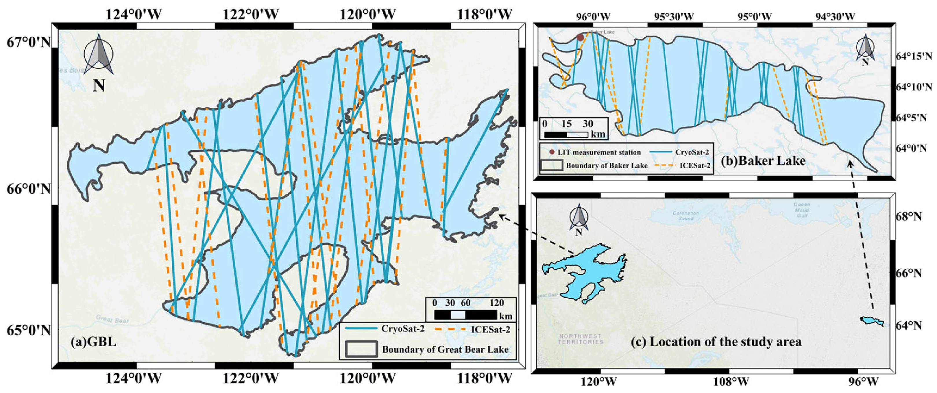
To address the limitations identified in previous studies, this study designed an LIT retrieval algorithm that combines ICESat-2 and CryoSat-2. ICESat-2 laser altimetry data are used to obtain the surface elevation values of the lake ice. Then, the high-precision surface elevation values of the lake ice are used to assist in peak identification in CryoSat-2 waveforms. In contrast to the peak identification method with the empirical fixed-range bin, the proposed method dynamically adjusts the position of the range bins based on ICESat-2 data, thereby possessing clear physical significance. Furthermore, the ice thickness retrieval experiments were conducted on Baker Lake and GBL during winter. The results indicate that the proposed method achieves a high precision in ice thickness retrieval.

The remainder of this article is arranged as follows. Section 2 provides an overview of the study area. Section 3 introduces the various types of data used in the article. Section 4 explains the data preprocessing and the proposed lake ice retrieval method. Section 5 presents the lake ice retrieval experiments and compares and analyzes the results. Section 6 concludes the article.

2. Study Area and Data

2.1. Study Area

This study investigated two lakes in Canada: Baker Lake and GBL. Baker Lake is located in the north-central part of the Nunavut district, at a latitude of 64°N and longitude of 94–96°W (Figure 1b), with a length of 82.51 km from east to west, a width of approximately 62.38 km from north to south, and a surface area of 1888 km². Winters are cold and long, and temperatures are low all year round, with average winter temperatures reaching −30 °C. According to the measured data, Baker Lake is covered by lake ice from November to June of the following year, with an average LIT of about 1.45 m and a maximum LIT of more than 2 m. Meanwhile, Baker Lake is the largest lake among the existing LIT measurement stations in Canada which is suitable for observing on a large scale by remote sensing. GBL is the largest lake in Canada and the fourth-largest lake in North America. It is situated in the northern part of Canada approximately 65–67°N and 118–123°W (Figure 1a). There are many small islands in the lake. The lake shape is irregular, approximately 322 km long and approximately 40–175 km wide, with a lake surface area of 31,153 km², and a shoreline of up to 2719 km. The lake is relatively deep, with an average depth of 137 m and a maximum depth of 413 m. The maximum LIT in GBL was approximately 1.5 m from October to June of the following year [19], and the lake became navigable after mid-July. The GBL area is large enough and can respond significantly to climate change, and ice thickness studies of GBL are a research interest [9,10,11,16,17].

2.2. Data

This study primarily utilized ICESat-2 and CryoSat-2 altimetry data, as well as field measurements from Baker Lake. The selected study period was from winter 2021 to spring 2022 (

Table 1. Overview of major datasets in this study.

	Study Area	Period	Instrument
A	Baker Lake	7 November 2021–3 May 2022	CryoSat-2
		16 November 2021–27 April 2022	ICESat-2
B	GBL	2 December 2021–4 April 2022	CryoSat-2
		30 November 2021–2 April 2022	ICESat-2
C	Baker Lake	27 November 2021–15 April 2022	On-site measurement

), during which the study area was covered by lake ice, facilitating result validation.

2.2.1. CryoSat-2 Altimetry Data

CryoSat-2 is a radar altimetry satellite launched by the ESA in April 2010 [20]. The primary payload for altimetry carried by a satellite is SAR Interferometric Radar Altimeter (SIRAL). This radar altimeter has three measurement modes: low-resolution mode (LRM), synthetic aperture radar (SAR), and state-of-the-art dual-channel synthetic aperture interferometric radar (SARIn) [21]. Within the GBL region, CryoSat-2 operates in SARIn mode, in which the processor avoids the effects of terrain relief in the along-track direction with a footprint size of approximately 0.5 km². Moreover, within the Baker Lake region, CrySat-2 operates in LRM mode. The track of the CryoSat-2 data used in this study is shown in Figure 1.

2.2.2. ICESat-2 Altimetry Data

On 15 September 2018, NASA successfully launched the ICESat-2 satellite, which carried an Advanced Topographic Laser Altimeter System (ATLAS) payload [22,23]. ATLAS uses a six-beam laser to detect the ground, with two beams as a group; each group has a strong and weak laser beam, and the energy ratio of the strong and weak laser beams is approximately 3:1. Figure 2 shows the position of the six laser beams of ATLAS, perpendicular to the direction of the flight path; the distance between each pair of laser beams is 3.3 km, and the strong and weak laser beams in each group are 90 m apart. The combination of strong and weak laser beams allows the laser to obtain sufficient return photons on both bright and dark surfaces, and the three groups of strong and weak beams form a cross-measurement that can effectively improve the detection of the slope and change in ground surface elevation. ICESat-2 data products are available to the public in HDF5 format and are classified into four levels: 0, 1, 2, and 3, among which the ATL06 product provides land ice ellipsoid elevation. The track of the ICESat-2 data used in this study is shown in Figure 1.

2.2.3. On-Site Measurement Data

On-site measurements of LIT were obtained from the Canadian Ice Thickness Program (https://www.canada.ca/en/environment-climate-change, accessed on 27 January 2024), which was divided into the “Original Ice Thickness Program Collection” and the “New Arctic Ice Thickness Program”. The “original ice thickness program” comprises ice thickness and snow depth measurements collected at 195 stations. However, the program was discontinued in 2002. The latter began in the fall of 2002 and continues to the present day, but with a significantly reduced number of stations. Existing ice thickness measurement programs measure LIT at the same sites each year, starting when the ice is safe to walk on after the lake has frozen over and continuing until the ice breaks up, with measurements taken at 1-week intervals. The locations of the measure station at Baker Lake are marked with a red origin in Figure 1b. Measurements are conducted approximately once a week at the same location each year, starting from when the ice is safe to walk on after freezing and continuing until the ice cracks or becomes unsafe. The ice thickness is measured using either a special auger kit or a hot wire ice thickness gauge. The depth of snow on the ice at the measurement locations is also measured and reported, with accuracy to the nearest centimeter. There are no sites on GBL where the LIT is measured, and this study extends the use of the method to GBL to demonstrate its generalizability.

Temperature data were obtained from the Canadian Historical Climate Data website (https://climate.weather.gc.ca/historical_data, accessed on 27 January 2024), which provides access to historical weather and climate data and related information across Canada.

2.2.4. Lake Mask Data

The Global Self-consistent, Hierarchical, High-resolution Geography database [24] (https://www.soest.hawaii.edu/pwessel/gshhg, accessed on 27 January 2024) was used to determine the exact extent of the lake to screen laser point cloud data for footprints within the lake as well as radar altimetry data. The database contained data at five different resolutions, and the highest-resolution data were used to accurately map the boundaries of the lake.

3. Method

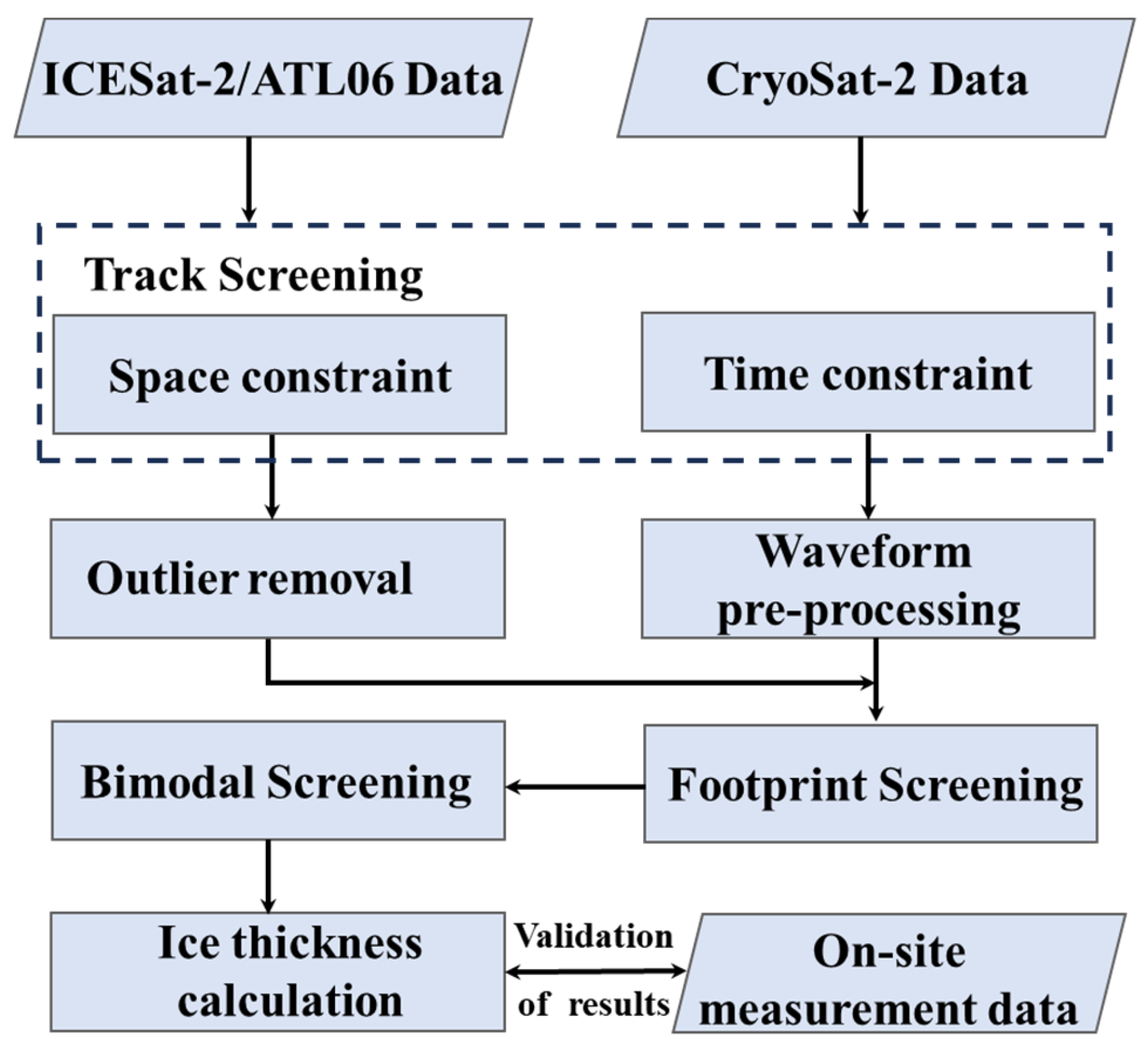
The proposed workflow of the LIT retrieval method using ICESat-2 to assist CryoSat-2 echo peak selection is shown in Figure 3. Suitable ICESat-2 and CrySat-2 tracks were screened based on spatial constraints and time restrictions. The characteristics of the ICESat-2/ATL06 data in the study area were then analyzed. We used a combination of global and local strategies to remove elevation anomalies from the ATL06 data to obtain more accurate elevation information on the lake ice surface. Simultaneously, we pre-processed the waveforms and analyzed their characteristics of CyroSat-2 waveforms above the lake ice during different seasons. Upon analysis of the lake ice structure and the radar waveforms, we found that there were obvious bimodal features in the radar echoes owing to the effects of snow–lake–ice surface reflections as well as lake–ice–water reflections. We screened the ICESat-2 and CryoSat-2 footprints that satisfied the distance conditions, found the sampling points in the CryoSat-2 waveforms corresponding to the ICESat-2 elevations, selected a suitable range window around the sampling points, and identified the echo bimodal feature points according to the energy limitation within the window, thus realizing LIT retrieval.

3.1. Pre-Processing

3.1.1. Track Screening

When dealing with satellite altimetry data with relatively sparse tracks and a long revisit period, time constraints and space constraints were used to screen out similar track data between two satellites to obtain a dataset with high relevance. The maximum distance between tracks and maximum separation time were set above the same lake to achieve this purpose. The maximum separation distance is a vital threshold used to determine whether the tracks of two satellites overlap spatially. If the tracks of the two satellites have moments above the lake that are less than the maximum distance, the two tracks are considered spatially coincident and can be retained. The maximum separation time is the maximum time between observations from the two satellites. If it is less than this threshold, the observations are considered to coincide in time. The simultaneous application of the maximum separation distance and maximum separation time constraints contributes to produce similar track data between the two satellites for subsequent data analysis and comparison. This approach can filter datasets with high spatial and temporal correlations for better LIT retrieval.

3.1.2. ICESat-2 Data Pre-Processing

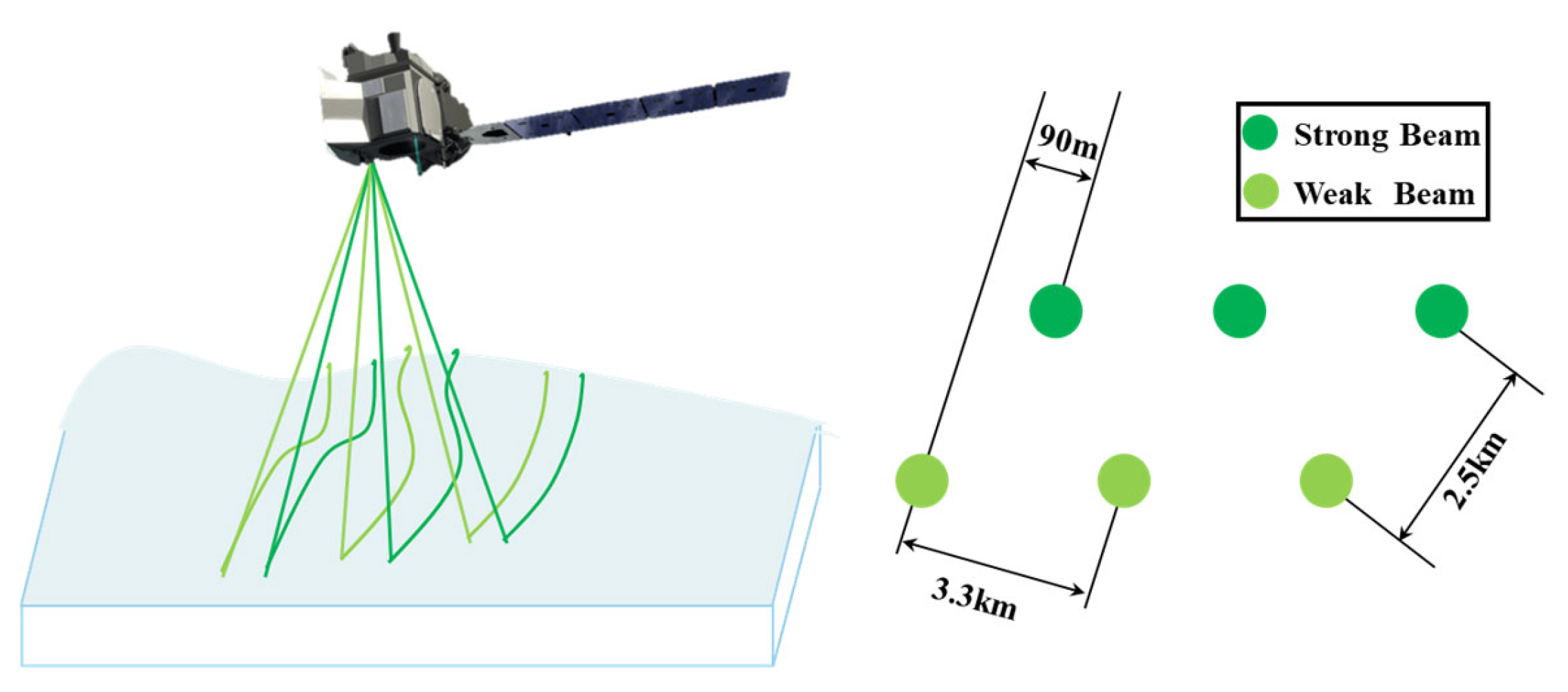
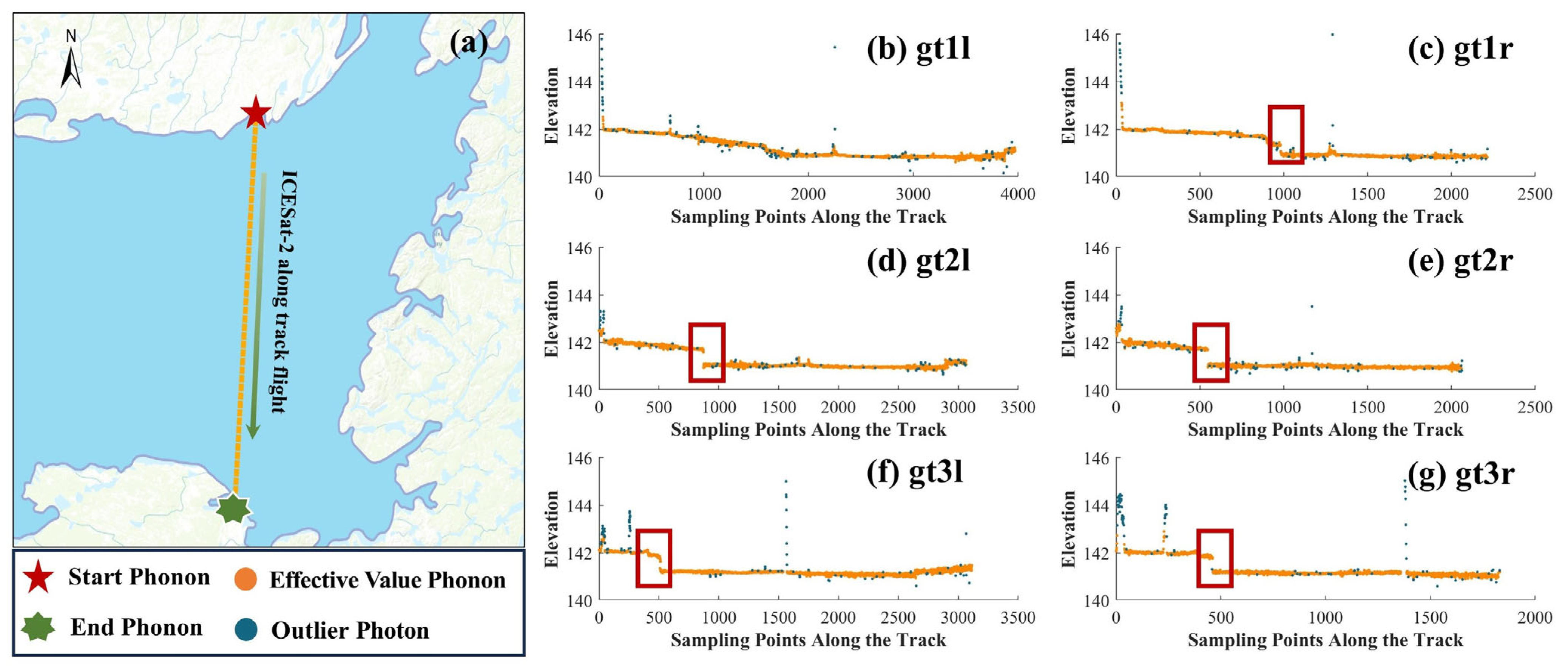
We used the ICESat-2/ATL06 data products in this study. ATL06 was generated using signal photons identified by ATL03 to produce land ice heights at fixed 20 m along-track intervals, with elevations generated from the median of signal photons within a 40 m range (overlapping each other by 20 m) [25]. Figure 4 shows the freeze-period lake ice surface elevation information obtained from the ICESat-2 satellite, and the subfigure (a) presents a satellite track across GBL. ICESat-2 flies backward, with the left beam indicating a strong beam and the right beam indicating a weak beam. From Figure 4b–g, we can see that the surface of the lake ice is relatively flat; however, we can still see a sudden change in height along the track distance direction, which is marked by a red rectangular box.

Although the ATL06 data have been filtered before the product release, the coarseness cannot be completely eliminated because the accuracy of the ATL06 data is mainly affected by factors, such as slope and cloudiness, and the elevation accuracy is reduced by an increase in slope [26]. A few anomalous data points deviate from the track elevation in Figure 4b–g (the blue dots are outlier photons), and it is necessary to eliminate the anomalous elevation data to obtain the accurate lake ice surface elevation information. In this study, two statistical methods were utilized to reject the outliers in ATL06. (a) For the entire track, data that were above the upper quartile or below the lower quartile by more than 1.5 times the interquartile range were labeled as outliers. This method is effective for removing outliers from data that are not normally distributed. (b) To detect local outliers, a method is used in which data points deviating from the local median by more than three times the median absolute deviation (MAD) within a certain window length are marked as outliers. For a random variable A composed of N scalar observations, the MAD is defined as

$$\mathrm{MAD}=\mathrm{median}\left(\left|A_i-\mathrm{median}\left(A\right)\right|\right),i=1,2,\dots ,N$$

(1)

A combined global and local strategy was used to remove outliers in the ATL06 data above the lake ice, with blue dots indicating elevation outliers and yellow dots indicating valid elevation values in Figure 4b–g, showing that this strategy can accurately remove most of the outliers.

3.1.3. CryoSat-2 Data Pre-Processing

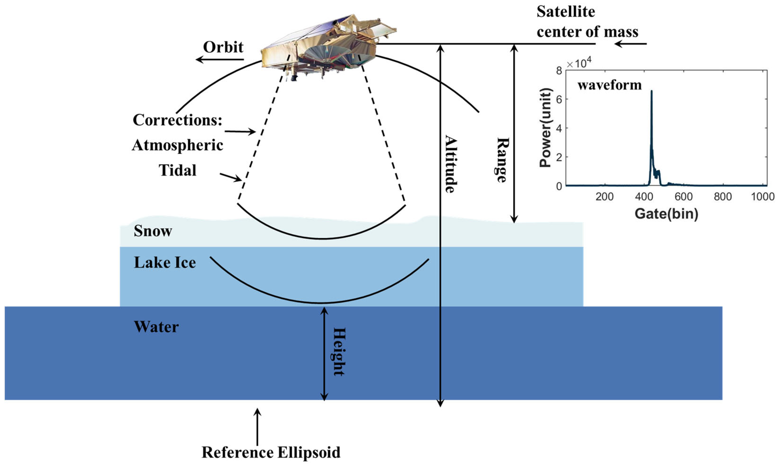
The radar altimetry satellite emits radar pulses toward the Earth’s surface and measures the distance between the satellite and the reflecting surface by receiving echoes. The surface elevation can be obtained using a distance conversion process. Figure 5 illustrates the altimetry principle of CryoSat-2 and provides an example of a typical echo produced on the surface of a frozen lake. In the vertical dimension, CryoSat-2 can only receive echoes within a “range window” specified by the width of the spectrum. In the new version of the CryoSat-2 L1B level data, the range window corresponded to 1024 sampling points for the SARIn mode and 128 for the LRM mode [27,28].

According to Figure 5, the ellipsoidal height of the target producing the echo can be calculated as follows:

$$H=Alt-R-C$$

(2)

where H denotes the ellipsoid height. Alt denotes the distance between the center of gravity of the satellite and the reference ellipsoid WGS84, R denotes the range between the target generating the echo and the satellite, and C denotes all range corrections required.

For sampling point n, the range R(n) between CryoSat-2 and the target generating the echo are calculated using the following equation:

$$\begin{array}{l}R\left(n\right)=\frac{T_{w}c}{2}-\frac{N_{s}c}{8B}+\frac{nc}{4B}=\frac{c}{8B}\left(4T_{w}B-N_s+2n\right)\\ N_s=\left\{\begin{array}{l}128, \mathrm{LRM}\\ 256, \mathrm{SAR}\\ 1024, \mathrm{SARIn}\end{array}\right.\end{array}$$

(3)

where $T_w$ denotes the distance delay from the center distance gate, given as parameter window_del_20_ku in the CryoSat-2 data, c denotes the speed of light in vacuum, B is the bandwidth obtained from the measurements, here taken as $B=320 \mathrm{MHz}$, and $N_s$ is the number of range window sampling points associated with the measurement mode. Notably, we used the speed of light in a vacuum to calculate the range, which is only a rough approach to determine the range window and does not conflict with the method of calculating the LIT later in the paper.

Because of the refractive properties of the atmosphere, radar pulses are slightly slowed down when they pass through the Earth’s troposphere. When the speed of light in a vacuum is used to convert the time delay to the distance bias, many range corrections must be made to remove this slight additional delay. Tidal corrections are also required to correct for the effects of tidal factors on satellite altitude.

$$\begin{array}{l}C=C_{dry}+C_{wet}+C_{iono}+C_{inv bar}+C_{DAC}\\ \hspace{1em} +C_{oce}+C_{oce eq}+C_{load}+C_{solid}+C_{pole}\end{array}$$

(4)

Range corrections can be divided into two main parts [18]. The first row of Equation (4) on the right side represents atmospheric corrections; from left to right, they are dry tropospheric, wet tropospheric, ionospheric, inverse barometric, and dynamic atmospheric corrections. The second row represents tidal corrections; from left to right, they are the ocean tide correction, the long-period equilibrium tide correction, the ocean loading tide correction, the solid earth tide correction, and the geocentric polar tide correction. All correction values were obtained from the CryoSat-2 products.

The radar waveforms received above lake ice by different altimetry radar systems exhibited different features. For example, the waveforms of the traditional nadir-pointing radar altimeter (TOPEX/Poseidon-Jason series) above lake ice show less pronounced bimodal peaks with very long trailing tails [18], which is quite different from the waveforms exhibited by CryoSat-2 in the SARIn mode [16].

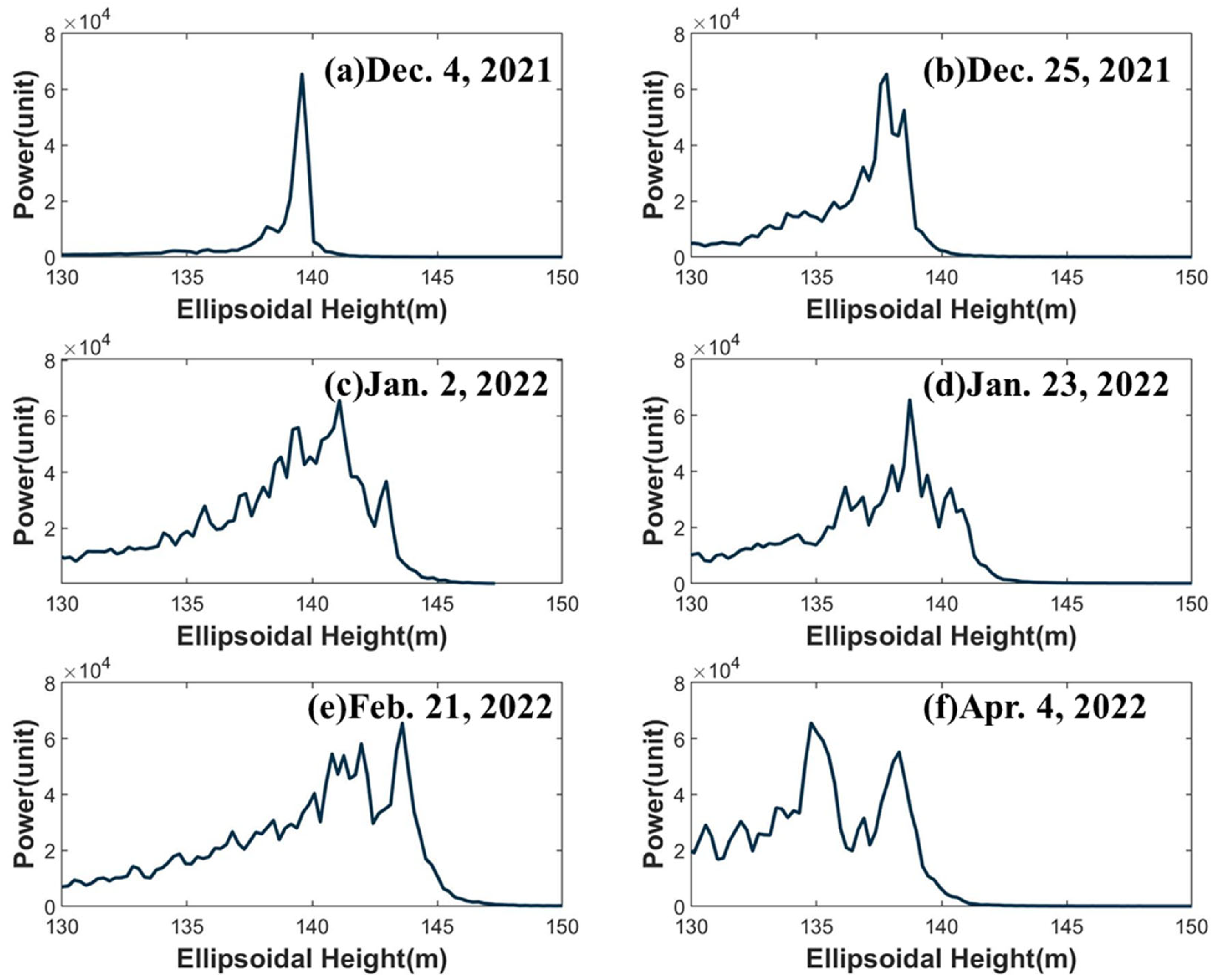
Figure 6 illustrates the echo waveforms of CryoSat-2 above GBL during different periods. Figure 6a shows an echo from 4 December 2021, which shows a clear single peak. It is possible that GBL is not fully frozen during this period, causing such a single peak. Figure 6b shows the echo from 25 December 2021. It is clear that the echo has two prominent peaks when the lake is completely frozen. However, in Figure 6c, three distinct peaks are visible: two are very high and one is relatively low. By 23 January 2022, the lake ice had grown thicker, and Figure 6d shows more complex peak features. As shown in Figure 6e,f, the LIT grows quite thick, but it is difficult to determine the snow-lake ice surface reflection as well as the lake ice-water body reflection points. In addition, by combining the data from multiple tracks, we observed that the peaks appeared at different elevations, which makes it challenging to identify peak feature points.

3.2. ICESat-2-Assisted CryoSat-2 Echo Peak Selection

By combining Figure 5 and Figure 6, we can see that above the lake surface in winter, the electromagnetic waves emitted by the radar altimeter satellite undergo multiple scattering because of the influence of layered media, such as lake water, lake ice, and snows. The difference in the scattering location is reflected in the echo to produce multiple peaks. The main challenge in using radar waveform analysis to retrieve LIT is correctly identifying the feature points of the echo peaks. Previous methods assumed that peaks appeared within a fixed-range bin [16]. However, owing to variations in lake water levels and fluctuations in the surface elevation of the lake ice, this method performed differently in different lakes.

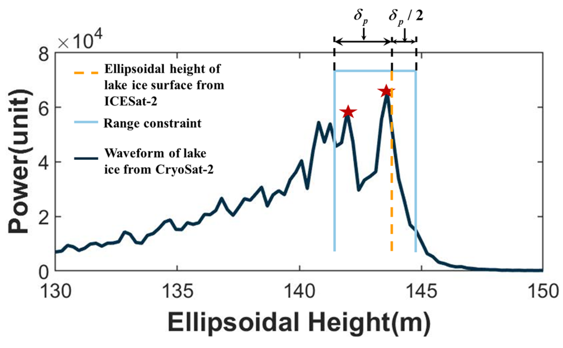
It is known that ICESat-2 can measure elevations with very high precision (<0.1 m elevation accuracy in smooth areas); therefore, we can use ICESat-2 to determine the ellipsoidal height of the lake ice surface. At the same time, we can calculate the elevation corresponding to each sampling point within the range window of CryoSat-2. By identifying the sampling points corresponding to the ellipsoid height of the lake ice surface, we can select a narrower range window around these points, such that the peak echo feature point will necessarily be within this window, thereby limiting erroneous peak detection.

We determined the size of the range constraint window based on the maximum thickness of the lake ice that electromagnetic waves can penetrate. Assuming the elevation of the lake ice surface is $h_{\mathrm{elli}}$ and the maximum thickness of the lake ice that the electromagnetic wave can penetrate is ${\delta }_p$, then the size of the range constraint window is set as $\left[h_{\mathrm{elli}}-{\delta }_p,h_{\mathrm{elli}}+{\delta }_p/2\right]$.

This method requires the observation points of CryoSat-2 and ICESat-2 to be sufficiently close in space to avoid the influence of undulations on the lake ice surface. We used Equation (5) to limit the distance between the footprint points of CryoSat-2 and ICESat-2.

$$\mathrm{L}\left[P_{\mathrm{CS}2}\left(\phi ,\theta \right),P_{\mathrm{IS}2}\left(\phi ,\theta \right)\right]<{\mathrm{T}}_{\mathrm{dist}}$$

(5)

where $P_{\mathrm{CS}2}\left(\phi ,\theta \right)$ and $P_{\mathrm{IS}2}\left(\phi ,\theta \right)$ are the latitude and longitude coordinates of the observation points of CryoSat-2 and ICESat-2, respectively; $\mathrm{L}(·)$ denotes the function used to determine the distance between the two coordinates; and ${\mathrm{T}}_{\mathrm{dist}}$ is the distance threshold between the two observation points. We averaged all the ICESat-2 elevation values that satisfied Equation (5) as the elevation values of the CryoSat-2 footprint points.

Under ideal conditions, there are usually only two peaks within the range constraint window. However, due to the complex environment of the lake ice surface, there may be more than two peaks within the range window. To effectively identify the peak feature points caused by the reflection of the upper and lower surfaces of the lake ice, we adopted the following strategy. We assumed that the most significant peak within the range constraint window was necessarily caused by the reflection of the snow–ice interface or the ice–water interface. Therefore, we considered the most significant peak point within the range constraint window as the feature point. For the second peak feature point, the peak point that appeared first within the range constraint window was searched. If the first peak that appeared was the maximum peak, we selected the second-most prominent peak as the second peak feature point. To ensure that the selected second peak point has sufficient distinctiveness, an energy constraint needs to be satisfied, which means that the peak value of the second peak point must be no less than 0.5 times the maximum peak value. Figure 7 shows a schematic diagram of filtering peak feature points with the above method, and this range constraint window method effectively avoids the identification of erroneous peak points.

3.3. LIT Calculation

In the previous section, we identified two peak feature points in the waveforms of the two echoes. Based on the interaction mechanism between electromagnetic waves and ices, we can calculate the thickness of the lake ice. When electromagnetic waves propagate in a medium, energy loss, known as attenuation, inevitably occurs. Simultaneously, as electromagnetic waves traverse a medium, the atoms or molecules within the medium undergo excitation in response to the electromagnetic field, subsequently emitting new electromagnetic waves. This phenomenon results in a reduction in the propagation velocity of electromagnetic waves within the medium. The complex dielectric constant is commonly used to characterize the electromagnetic properties of a medium [29]. The real part of the relative permittivity is represented by ${\epsilon }_r^{\prime }$, and the imaginary part is represented by ${\epsilon }_r^{″}$. The real part ${\epsilon }_r^{\prime }$ corresponds to the dielectric constant without attenuation, whereas the imaginary part ${\epsilon }_r^{″}$ represents the energy attenuation. Between 10 MHz and 300 GHz, the real part ${\epsilon }_r^{\prime }$ of the dielectric constant of ice is temperature-dependent [30]:

$${\epsilon }_r^{\prime }=\left\{\begin{array}{l}3.1884+(9.1·{10}^{-4})·T_i\hspace{1em}-30 °\mathrm{C}\le T_i\le 0 °\mathrm{C} \\ 3.1\hspace{1em}\hspace{1em}\hspace{1em}\hspace{1em}\hspace{1em}\hspace{1em}\hspace{1em}\hspace{1em}\hspace{1em}{T}_i\le -30 °\mathrm{C}\end{array}\right.$$

(6)

The propagation velocity $v$ of an electromagnetic wave in a medium can be calculated using Equation (7):

$$v=\frac{c}{\sqrt{{\epsilon }_r}}$$

(7)

where $c$ is the speed of propagation of light in vacuum $c=2.997924562\times {10}^8\mathrm{m}/\mathrm{s}$ and ${\epsilon }_r$ are the dielectric constants of the medium.

In the previous section, we identified the peak feature points in the CryoSat-2 echoes using the ICESat-2-assisted method. By combining the penetrative properties of electromagnetic waves in ices and snows, we can calculate the thickness of the lake ice.

$$\begin{array}{l}{h}_i=v·\Delta t=v·\frac{\Delta P}{2·nB}\\ n=\left\{\begin{array}{l}1, \mathrm{LRM}\\ 2, \mathrm{SAR}/\mathrm{SARIn}\end{array}\right.\end{array}$$

(8)

where $v$ represents the radar penetration speed in ices and snows, $\Delta P$ is the sampling range between two peak feature points, and B is the bandwidth. Along a track, we retrieved the LIT corresponding to each echo and averaged the LIT on this track to obtain the LIT at the time of the track crossing.

3.4. Validation of Results

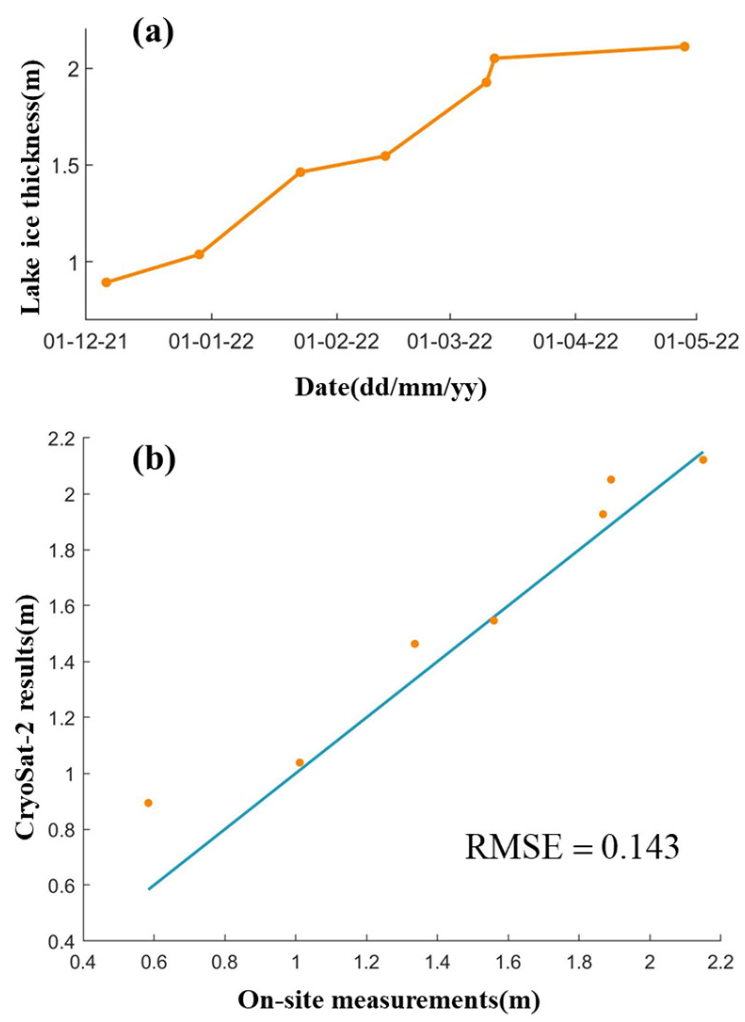
The validation of satellite-based altimeter retrieval results has always been a complex and challenging problem in the field of remote sensing. For the two study areas, there is only one lake ice measurement station in Baker Lake, which can be used as a basis for quantitative assessment of the retrieval results. Therefore, this paper only quantitatively evaluates the results at Baker Lake and qualitatively analyzes the results at GBL.

Although there is a measurement station in Baker Lake, the large footprint and sparse track of CryoSat-2 make it difficult to guarantee that all orbit data cover the measurement station. Therefore, it becomes challenging to validate the retrieval results at the measurement station [31,32]. Meanwhile, cross-validation is also complicated due to the difficulty in obtaining other satellite data transiting the study area in the same time series [33]. According to the characteristics of lake ice, the lake ice thickness should remain stable in the same area, but sudden changes in ice thickness may occur due to grounding/deformation, which are reflected as outliers in the retrieval results. To improve the accuracy of result evaluation, the average LIT is used for result validation. The performance of the three ice thickness retrieval methods is compared by calculating the root mean square error (RMSE) to evaluate their advantages and disadvantages.

$$\mathrm{RMSE}=\sqrt{\frac{{\displaystyle \sum _{i=1}^n{\left(h_{m,i}-h_{r,i}\right)}^2}}{n}}$$

(9)

where $h_{m,i}$ represents the measured data and $h_{r,i}$ represents the satellite retrieval results.

For GBL, due to the lack of on-site measurement data, we are unable to quantitatively evaluate the accuracy of the results. However, we have extensively utilized meteorological data for qualitative analysis to validate the trend of GBL LIT during the study period. This qualitative analysis can provide a certain level of result validation, although it cannot provide precise numerical comparisons. In the absence of measured data, utilizing meteorological data for trend analysis remains an effective approach, which helps validate the rationality and reliability of the model or remote sensing retrieval results.

4. Result

4.1. Retrieval Results

According to the methodology of this paper, the retrieval of the winter lake ice thickness in Baker Lake and GBL has been carried out, of which part results are shown in Figure 8. From the results, we can observe that, whether in Baker Lake or GBL, the retrieved ice thickness exhibits fluctuations but overall tends to be stable along the same track. In Baker Lake, there are clearly several outliers in the ice thickness. Due to the lack of actual measurement data, we are currently unable to determine the specific reasons for these outliers. It could be caused by deformation and compression of the lake ice or data quality issues. Therefore, in subsequent evaluations, averaging the results is necessary to ensure the validity of the assessment.

At the same time, most of the retrieval results show a peak-like shape. In the first part of each track, the ice thickness tends to increase, while in the latter part of each track, the ice thickness tends to decrease. This may be due to the smaller ice thickness near the shore and thicker ice thickness in the middle of the lake. Such trends demonstrate the complexity of lake ice structure and provide valuable information for further understanding the distribution of lake ice thickness.

4.2. Algorithm Performance

We verified the feasibility and accuracy of our method by retrieving LIT from Baker Lake. In Figure 9a, the vertical axis represents the retrieved LIT values and the horizontal axis represents the dates when CryoSat-2 passed over Baker Lake. The orange dots show the growth trend of the LIT. In Figure 9b, the retrieval results of the lake ice in Baker Lake are compared with the on-site measurements. The RMSE between the retrieved results and on-site measurements was 0.143 m, indicating good accuracy. When the LIT was 1–2 m, there was a strong correlation between the retrieved results and on-site measurements. However, during the initial freezing period, there was a large deviation in the retrieved results, which may be due to the presence of water on the lake ice surface. The water blurs the echo peaks of CryoSat-2 and poses the misidentification of peak features.

5. Discussion

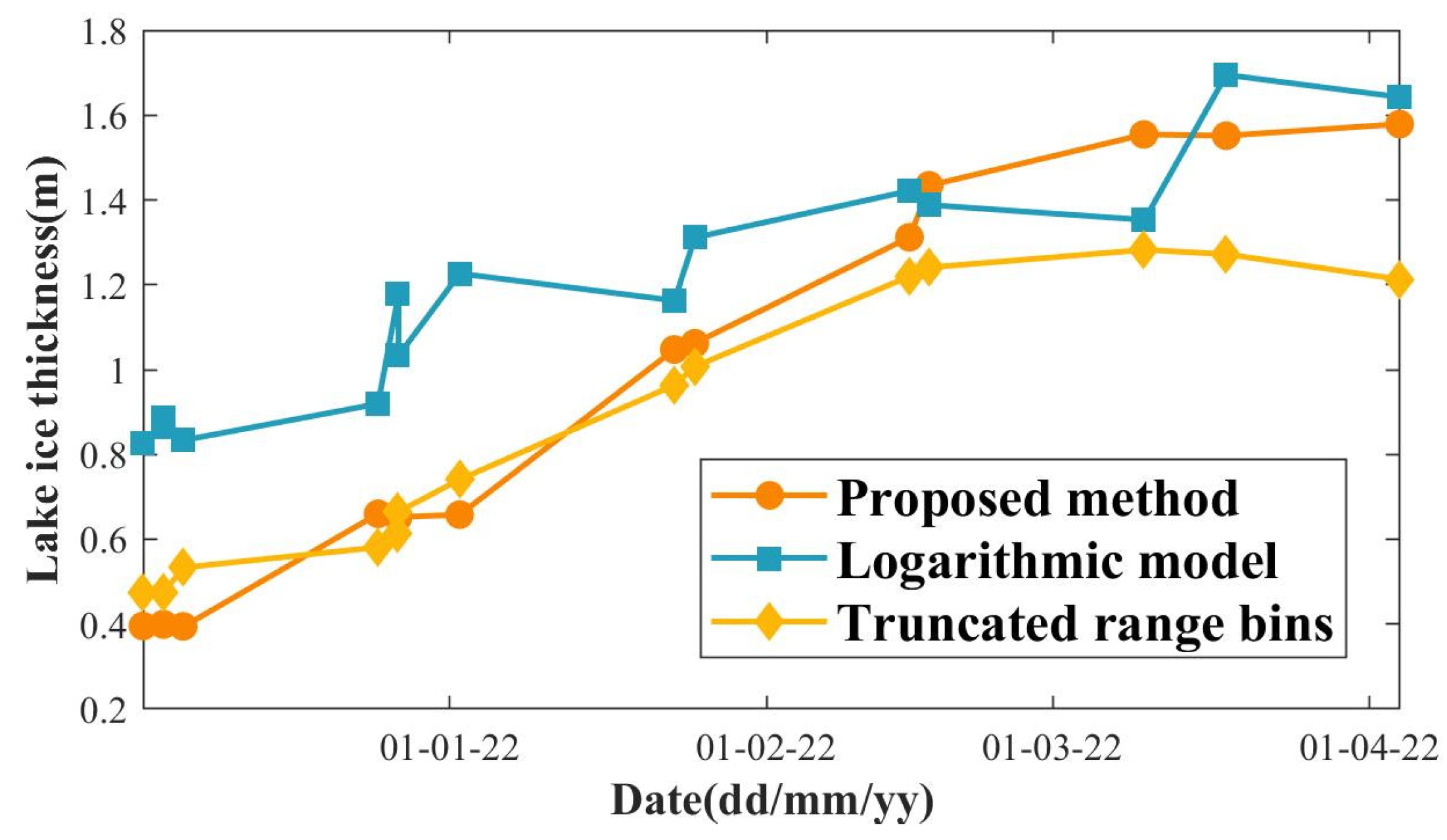
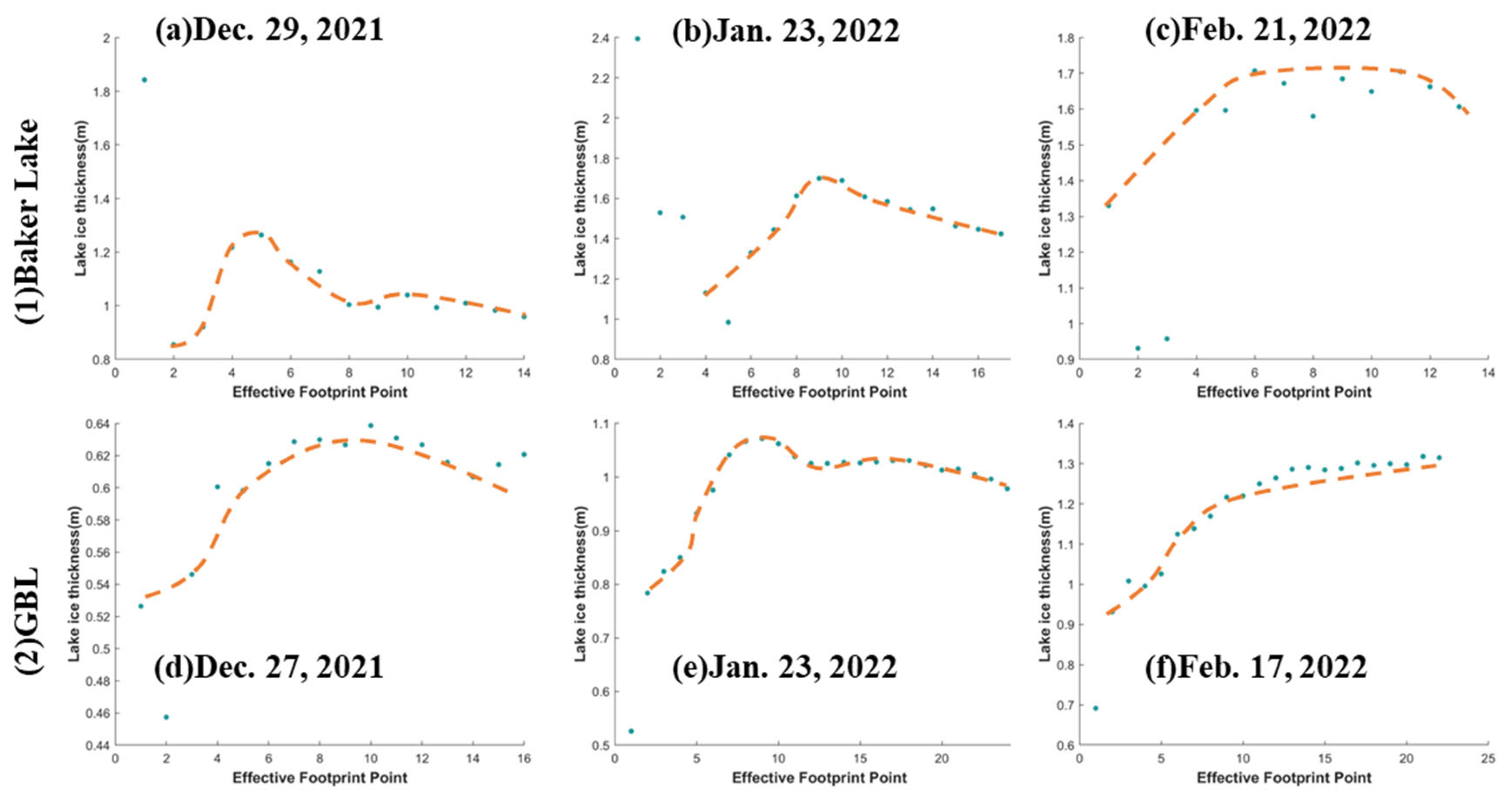
In this section, the proposed method is compared with two other methods. One method utilizes the backscattering coefficient for LIT retrieval [15], whereas the other uses a fixed-range bin for LIT retrieval [16]. By comparing the two methods, we evaluate the performance of the proposed method for LIT retrieval. Figure 10 shows the results of the LIT retrieval for Baker Lake using the three methods.

Table 2. The results of the three methods for LIT retrieval in Baker Lake are as follows.

Date	Logarithmic Model	Fixed Range Bins	Proposed Method	On-Site Measurements
6 December 2021	1.10	1.08	0.89	0.58
29 December 2021	1.07	1.03	1.04	1.01
23 January 2022	1.14	1.49	1.46	1.34
13 February 2022	1.18	1.65	1.55	1.56
10 March 2022	1.23	1.44	1.93	1.87
12 March 2022	1.24	1.77	2.05	1.89
28 April 2022	1.55	1.68	2.12	2.15
RMSE	0.48	0.32	0.14

provides detailed results as well as quantitative evaluations for each method. It can be observed that the proposed method achieved the highest accuracy and performed the best. The logarithmic model exhibits the lowest accuracy, possibly due to the unsuitability of the parameters in the logarithmic regression model. The fixed-range bin method yields poor retrieval results, possibly because some peak features are not within the fixed-range bin, leading to the incorrect identification of peak features and a decrease in retrieval accuracy.

Using only the backscattering coefficient and a regression model for LIT retrieval in the lakes, the regression model parameters were calculated using the measured data. However, this method is not applicable to lakes that lack measurement data. Owing to the potential differences in the physical and environmental characteristics of lakes, the direct application of the model parameters of one lake may result in decreased performance. It is assumed that the peak feature point appearing within a fixed-range bin is highly unreasonable and may lead to incorrect identification. In contrast, the proposed method adopts a strategy based on the identification of peak feature points using ICESat-2-assisted CryoSat-2 by dynamically adjusting the possible range of the peak feature points. This strategy improves the accuracy of the feature point identification and effectively enhances the precision of LIT retrieval.

GBL has no station to measure its ice thickness, but it is an essential lake in the sub-Arctic region. Therefore, it is indispensable to retrieve its ice thickness by the remote sensing method. GBL is a relatively large lake with slow ice growth, and its ice is thinner than that of Baker Lake, making its retrieval more challenging. However, the proposed method demonstrates good retrieval accuracy and provides valuable references for the GBL ice thickness. Figure 11 shows the retrieval results of GBL using different methods, indicating varying outcomes, but with similar trends. According to the latitude and temperature of GBL, the initial freezing period occurred from November to December. As the temperature increased, ice melting began, and the thickness decreased until May of the following year. The results obtained using the proposed method align with the seasonal variations in GBL, enhancing its credibility.

6. Conclusions

This study proposes a novel method for retrieving LIT, which uses ICESat-2-assisted CryoSat-2 waveform peak selection and validation through on-site measurement data. The method demonstrates excellent accuracy and can be applied to lakes without on-site measurement data. In the proposed method, effective ICESat-2 and CryoSat-2 tracks were first selected based on spatio-temporal constraints. The ICESat-2/ATL06 level product was then pre-processed to remove outliers and obtain accurate lake ice surface ellipsoid heights. Next, the echo sampling points of CryoSat-2 were converted to their corresponding ellipsoid heights, and the range constraint window for the peak feature points was dynamically adjusted based on the measurement results of ICESat-2. Finally, accurate LIT retrieval results were obtained by combining the peak feature point selection strategy and LIT calculation formula.

On the experimental side, this study performed LIT retrieval for Baker Lake with on-site measurements. The feasibility and superior accuracy of the proposed method were verified by comparison with logarithmic retrieval models and fixed-range bin methods. Subsequently, the method was applied to GBL, which lacks on-site measurement data. The comparison with other methods in this study demonstrates that the proposed method has higher reliability. In the future, we will apply this method to other lakes to enhance its value and application scope.