Abstract
The Bidirectional Reflectance Distribution Function (BRDF) is a critical spatial distribution parameter in the quantitative research of remote sensing and has a wide range of applications in radiometric correction, elemental inversion, and surface feature estimation. As a new means of BRDF modeling, UAV push-broom hyperspectral imaging is limited by the push-broom imaging method, and the multi-angle information is often difficult to obtain. In addition, the random variation of solar illumination during UAV low-altitude flight makes the irradiance between different push-broom hyperspectral rows and different airstrips inconsistent, which significantly affects the radiometric consistency of BRDF modeling and results in the difficulty of accurately portraying the three-dimensional spatial reflectance distribution in the UAV model. These problems largely impede the application of outdoor BRDF. Based on this, this paper proposes a fast multi-angle information acquisition scheme with a high-accuracy BRDF modeling method considering illumination variations, which mainly involves a lightweight system for BRDF acquisition and three improved BRDF models considering illumination corrections. We adopt multi-rectangular nested flight paths for multi-gray level targets, use multi-mode equipment to acquire spatial illumination changes and multi-angle reflectivity information in real-time, and introduce the illumination correction factor K through data coupling to improve the kernel, Hapke, and RPV models, and, overall, the accuracy of the improved model is increased by 20.83%, 11.11%, and 31.48%, respectively. The results show that our proposed method can acquire multi-angle information quickly and accurately using push-broom hyperspectral imaging, and the improved model eliminates the negative effect of illumination on BRDF modeling. This work is vital for expanding the multi-angle information acquisition pathway and high-efficiency and high-precision outdoor BRDF modeling.
1. Introduction
The Bidirectional Reflectance Distribution Function (BRDF) is defined as the ratio of the irradiance in a given outgoing direction to the irradiance in a given incoming direction on that surface element, and this function can be used to characterize the surface reflectance anisotropy [1,2]. Currently, it is mainly applied to radiometric correction of satellite-borne instruments [1], radiometric correction of low-altitude images [3], light utilization, albedo inversion [4,5], crop mapping [6], crop element estimation [7], and estimation of metal surface roughness [8]. The modeling accuracy of the BRDF has directly impacted the application of quantitative remote sensing. In addition, random variations in illumination can directly affect the radiometric consistency of the raw multi-angle reflectance data, and BRDF modeling relies heavily on data quality. Therefore, the effective acquisition of multi-angle reflectance information and the random illumination variation significantly affect the BRDF modeling accuracy.
UAV multi-angle remote sensing of the ground has the advantages of flexibility and convenience, flexible imaging time, strong data acquisition ability in complex areas, and high spatial resolution [9] and has gradually become an essential means of BRDF data acquisition. Centimeter-level UAV equipment provides [10] platform support for surface aerial surveys; Tao et al. [11] used a UAV-carried spectrometer to take multiple shots of the Dunhuang radiation correction field, and the relative deviation of reflectance of the characteristic bands was within 5% and simulated the calculation of changes in the amount of solar radiation. However, there is still a slight error compared to the actual value. Latini et al. [12] demonstrated the consistency of the vegetation spectral dimensions by using a UAV to collect vegetation data at 90 m altitude and modeling the comparison of the BRDF with Sentinel satellite data. Still, the number of acquired images was small, and the illumination effect was not considered.
UAV-based hyperspectral imagers can be categorized into frame-amplitude and push-broom imaging modes. Framed imaging can utilize UAV hovering to collect multi-angle information at a fixed point on the target area to ensure the stability of the spatial structure and texture of the photographed target image. Still, acquiring images that consider spectral accuracy, spatial resolution, and spectral resolution simultaneously is challenging. Hovering imaging is not possible when using push-broom imaging, and the UAV must be controlled to push-broom along a straight line at a uniform speed to acquire multi-angle information [12]. Push-broom imagers have high signal-to-noise ratios (SNRs) and high spectral resolutions. Yet, they are seldom used to carry out the acquisition of multi-angle information and the modeling of the BRDF [13]. Considering that both spectral and spatial resolutions need to be considered for BRDF modeling, push-broom hyperspectral imagers can undoubtedly provide greater convenience for existing BRDF model building. However, the characteristics of push-broom imaging are more sensitive to the flight altitude of the UAV platform carried, so optimizing the multi-angle information acquisition method and tapping the potential of the push-broom hyperspectral imager in multi-angle information acquisition and BRDF modeling are of broad significance to ensure the accuracy of BRDF modeling and extend the data acquisition path.
Eliminating the effect of random variations in illumination on BRDF modeling is critical. When acquiring images of a target area using a UAV-borne hyperspectral imager, the flight altitude is generally located under clouds, and it takes time cycles to capture multi-angle information. The illumination changes over time during the cycle, which results in the acquired reflectance information being captured with inconsistent illumination [14]. Directly using such data with illumination bias for BRDF modeling, both the model parameters and reflectance inversion will produce large deviations, and the changes in illumination are generally random, making the random effects on BRDF modeling difficult to eliminate. Most existing research assumes the consistency of illumination radiation within a certain period and does not consider the impact of random changes in illumination [1,10,15,16,17,18,19,20]. However, if all hyperspectral images are corrected with the same atmospheric parameters, there is still a significant error in the model parameters [12]. Currently, there are two main methods to eliminate illumination; one is to eliminate it by synchronized monitoring of equipment [21,22,23], but there is no uniform method for this elimination process. The other is elimination by simulation [11] or model iteration [24], but when the random illumination variation lacks regularity, the data from the simulation loses its meaning. Model iteration requires ample data support in long time series, which is hugely inefficient. It is urgent to solve the problem of inconsistent irradiance due to illumination variations and thus improve the accuracy of BRDF modeling.
Models that characterize the BRDF can be classified as semi-empirical models, physical models, and statistical models. The general modeling approach uses the model prototype to invert the model parameters with the observation data and then perform the BRDF distribution in the target area [15,16,17,25,26]. For example, the prototype Kernel model can be used to invert the isotropic scattering, body scattering, and geometrical optics kernel coefficients in the model to obtain the reflectance distribution in 3D space with a small amount of observational data [27,28,29]. However, particular surface types often limit the applicability of the original model. Then, the improvement of the model is significant, such as the body scattering kernel that fully considers the hotspot effect [15], the snow kernel that characterizes the anisotropic reflectivity of snow [30], the terrain kernel for rugged terrain [31], etc., which have effectively extended the application of the kernel model. The Hapke model, as a physical model, maximizes the considerations of single scattering, multiple scattering, and hotspot effects for the application of this model mainly focuses on the quantification and calculation of each parameter, and its characterization ability also tends to depend on the accuracy of each parameter. The RPV model is a semi-empirical diametrically oriented reflectance model containing three parameters. The three parameters are the incident/observed reflectance in the zenith direction, the asymmetry factor, and the correction factor. The model is between the traditional semi-empirical and physical models, which retains a better fit and highlights the physical factors affecting the spatial albedo [28,29,31]. Therefore, the improvement based on the original BRDF model should explore the model’s potential while considering the applicability of different models to the improvement, reducing the difficulty of the improvement method and the complexity of the model.
The main contributions of this paper are as follows:
- Designed a multi-rectangle nested acquisition method applicable to push-broom hyperspectral imaging, utilizing a UAV-carried hyperspectral imaging system and ground-based auxiliary equipment to improve the access and efficiency of multi-angle information acquisition, including illumination.
- Acquired multi-angle hyperspectral images in the 400–1000 nm range, including 150 bands and multiple gray-level targets, and simultaneously acquired outdoor illumination changes.
- Model improvement by theorizing, normalizing, and introducing illumination variations into three BRDF models. BRDF modeling of multi-gray level targets using the improved models improves the ability of the models to characterize reflectance in three-dimensional space.
2. System and Methods
2.1. BRDF Data Acquisition System
BRDF modeling requires multi-angle reflectance information of the target region at different bands, including reflectance at the solar zenith angle (SZA), solar azimuth angle (SAA), observed zenith angle (VZA), and observed azimuth angle (VAA) [11]. The air and ground equipment cooperate to collect information systems from different angles as shown in Figure 1. Firstly, the coordinates of the imaging center are established, and the planned flight route of the UAV is written into the flight control software, relying on the coordinate positioning to realize multi-angle information acquisition under different VZAs and VAAs. A VZA contains 12 groups of data within 0–360° at 30° intervals, and the SZA and SAA are obtained by calculating the imaging time and latitude/longitude coordinates of the imaging center.
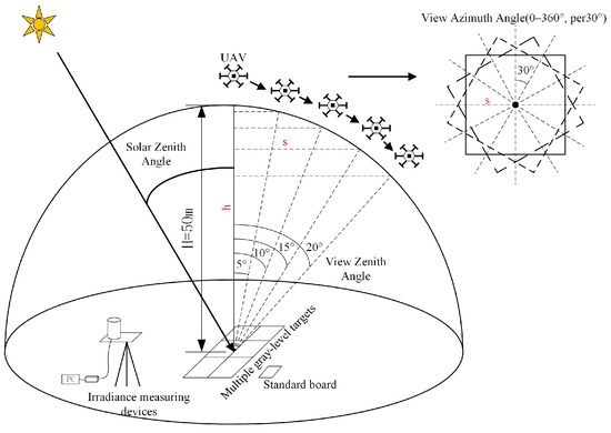
Figure 1.
BRDF data acquisition system.
This research utilizes a UAV platform, a stabilized gimbal, a hyperspectral imager, targets and standard plate, and a downward atmospheric irradiance measurement device to form a multi-angle BRDF acquisition system. For the flight equipment, the UAV uses a DJI M600 multi-rotor UAV (Shenzhen, China), and the hyperspectral imager uses a Corning push-broom hyperspectral imager (Corning, NY, USA) with the parameters in Table 1. The spectrometer is mounted on a DJI Ronin MX stabilized gimbal, suspended underneath the UAV, and the gimbal can be adjusted from 0° to 90° of the pitch angle as in Figure 2. The imaging principle of push-broom hyperspectral is shown in Figure 3.

Table 1.
Spectrometer parameters.
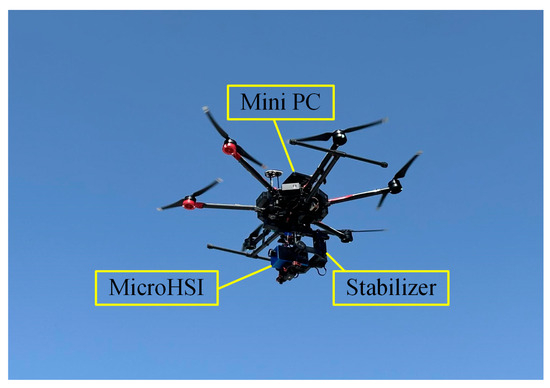
Figure 2.
UAV and auxiliary equipment.
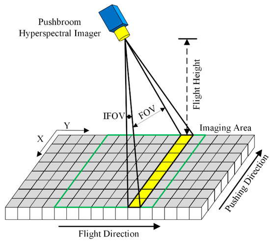
Figure 3.
Push-broom hyperspectral image.
For the ground equipment, the laying of a multi-gray level for the ground equipment, a multi-gray scale target, and a standard reflectivity plate are laid, and an atmospheric downward irradiance measurement device is set up as in Figure 4a, which consists of a spectrometer and a cosine corrector. The spectrometer uses the Ocean Optics USB2000+ (Dunedin, FL, USA), and the cosine corrector collects irradiance at a stereo angle of 180°. Multi-angle collection is achieved through UAV flight route planning, a hyperspectral imager is used to obtain multi-spectral reflectance information at different angles, multi-gray scale targets and a standard plate are used to provide reference and modeling data, and an irradiance measurement device is synchronized to monitor irradiance changes. The reflectance curves of the multi-gray level target and standard plate are shown in Figure 4b.
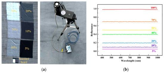
Figure 4.
Ground equipment. (a) Targets and irradiance measurement devices; (b) targets reflectance.
2.2. Reflectance Factor
The BRDF is a physical quantity that reflects the properties of the earth’s surface itself, independent of the measurement method. The strictly defined BRDF is unobservable, and the BRDF measurement is generally referred to as the measurement of the BRF or hemispherical directional reflectance factor (HDRF), which reflects the bidirectional reflectance properties of the earth’s surface. Numerically, there is a multiplicative relationship between the BRDF and BRF, as in Equation (1). In this paper, the measurement of the BRF is the main focus, and a hyperspectral imager is used to obtain data on the directional reflection of the target. A reference plate receives the outgoing illumination from the ideal diffuse reflective surface and calculates the target region’s reflectivity factor as in Equation (2).
where is the solar zenith angle, is the observation zenith angle, is the relative azimuth angle between the solar azimuth and the observation azimuth, is the corresponding wavelength, is the reflectivity factor of the target area, is the DN value curve of the target area, is the DN value curve of the standard plate, and is the reflectivity factor of the standard plate.
2.3. The Improvement of Models
By matching the hyperspectral push-broom imaging time and the atmospheric downward irradiance time, the downward irradiance corresponding to the shooting of each hyperspectral image frame can be obtained, and with the irradiance at a certain moment as a benchmark, the irradiance at all moments of the irradiance is normalized to obtain the illumination correction factor as in Equation (3):
where is a moment in time, is the corresponding wavelength, is the illumination correction factor, is the irradiance corresponding to the capture of each hyperspectral image frame, and is the irradiance at a moment in time during the UAV data collection. The DN value curve is corrected using the illumination correction factor as in Equation (4):
where is the corrected DN value curve.
The corrected DN value curve is obtained by substituting it into Equation (2):
where is the corrected reflectivity factor of the target area.
The Hapke model is formulated as
where is the bidirectional reflectivity, is the cosine of the incidence angle, is the cosine of the exit angle, is the phase angle between the incidence angle and the exit angle, is the single-scattering albedo, is the backscattering function, is the phase function, and is the multiple-scattering function.
The RPV model is formulated as
where , is the solar zenith angle and the observed zenith angle. , is the solar azimuth and observed azimuth, is the asymmetry factor with a value in the range of −1 to 1, determining the relative amount of forward and backward scattering. is the correction factor, is the incident and observed albedo in the zenith direction, is the scattering phase function, and is the hotspot effect term.
Kernel drive modeling formulas are
where , is the solar zenith angle and the observed zenith angle, is the relative azimuthal angle between the solar azimuth and the observed azimuth, is the corresponding band, is the bidirectional reflectivity, , is the volume scattering kernel and the geometric optics kernel, and , , is the coefficients of the isotropic scattering, volume scattering, and geometric optics kernel.
As in Equation (5), illumination correction factors are introduced into the three BRDF models as in Equations (9)–(11):
where , , are the bidirectional reflectance of the three models after correction. is the illumination correction factor.
2.4. Evaluation Method
The fitting ability of the three models and the model after introducing the illumination correction factor to the real data is evaluated comprehensively. Two aspects need to be considered: the fitting error within the model before and after improvement compared to the measured values and the comparison of the fitting error before and after improvement among the models. For the fitting error within each model, the Mean Square Error () and Root Mean Square Error (), as in Equations (12) and (13), are used to describe the fitting status. Scatter plots in polar coordinates between models were used to reflect the fitting differences between models.
where is the total number of spatial angle combinations, is the fitted value of the original or improved model, and is the measured true value.
To verify the change of the target in the spectral dimension after illumination correction, the spectral angle of the same target before and after illumination correction is calculated as Equation (14):
where is the number of sample points on the spectral curve, is the model fit value, and is the measured true value.
To calculate the model fit values, the least squares error method is used to inversely perform the model parameters by substituting the collected reflectance information under different combinations of angles into the model. The BRDF distribution of the target under any combination of angles is performed positively after obtaining the model parameters.
3. Experiment and Processing
3.1. BRDF Data Acquisition Scheme
The experiment was selected to be carried out under good weather conditions such as clear and less cloudy, sufficient illumination, and low wind speed. The UAV performed multi-flight and multi-angle acquisition and selected good-quality data for BRDF modeling.
Based on the imaging characteristics of push-broom hyperspectral imaging, the multi-angle information acquisition scheme required for BRDF modeling was designed, and the multi-angle refined BRDF data of the target area were obtained. The experimental site was chosen as the roof of a high-tech industrial park (34.09°N, 108.52°E); six different reflectance targets were laid in the target area, and a standard reflectance whiteboard was used to provide the reflectance data required for radiometric correction and BRDF modeling. This experiment collected 5° observation zenith angle data at intervals from 0° to 25°. The gimbal angle was adjusted to control the observation zenith angle of the UAV to ensure that the lens was always oriented to the target area. The 0° observation zenith angle data were first obtained by flying at the initial altitude of 50 m (red line track of the imaging area in Figure 5). The routine was adjust the route, fly to the starting position of the 5° observation zenith angle, start from the observation zenith angle of 5° at each observation zenith angle per the three rectangles nested route three times, fly a rectangle, and then fly the next rectangle, after each rectangle to fly to the start of the next rectangle route position (such as Figure 5, in turn flying the green, blue, and orange trajectory; the black solid dot represents the starting point of each rectangular trajectory). The three rectangles have equal side lengths, and the angle between adjacent rectangles is 30°. Each side length of each rectangle represents a set of observation azimuth data, and 12 sets of observation azimuth data can be obtained in intervals of 0–360° under one observation zenith angle. The flight trajectories under different zenith angles are the same. Only the altitude and traverse distance must be adjusted under each observation zenith angle (5° to 10° observation zenith angle in Figure 5). The length of the rectangle and the traverse distance are shown in Table 2. The calculation of the observation zenith angle, altitude, and traverse distance are shown in Equations (15) and (16). According to the data acquisition of this kind of flight trajectory, the original hovering imaging can be changed to motion imaging, and the characteristics of uniform velocity linear imaging of the swept-scan spectrometer can be considered. The change of the original hovering imaging to motion imaging can assess the characteristics of the push-broom spectrometer and acquire the BRDF modeling information with more decadent spectral bands and more accurate spatial angles. At the same time, it can also be used to construct several rectangular nested flight schemes with different pinch angles according to the demand to collect more refined data.
where is the initial altitude at 0° observation zenith angle, is the observation zenith angle, is the altitude corresponding to different observation zenith angles, and is the traverse distance corresponding to different observation zenith angles.
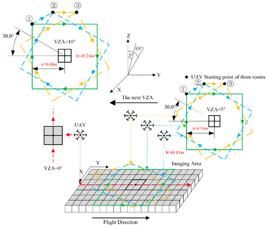
Figure 5.
UAV flight track. (the numbers ①, ②, and ③ represent the starting points of the three rectangular flight paths according to the flight order under each VZA).

Table 2.
VZA with aerial height and traverse distance.
The UAV acquires a complete hyperspectral image under one VZA in 3 to 5 min and reaches all preset VZAs in less than 20 min. We automated the chemical data collection as much as possible and conducted multiple experiments to ensure the high quality of BRDF modeling at the data level. During UAV hyperspectral data acquisition, the downward atmospheric irradiance measurement device captures changes in solar irradiance in different bands in real time. To match the image data acquired by the UAV hyperspectral, it is necessary to ensure that the irradiance acquisition is carried out throughout the experimental process, the sampling frequency must be greater than the shooting frequency of the hyperspectral image, and the spectral range includes the hyperspectral image spectral band. The acquired solar illumination variation data were processed by noise reduction and normalization to obtain the illumination correction factor. At the same time, the irradiance measurement device is spectrally equivalent to the hyperspectral image to ensure consistency in the spectral dimension [32]. For each spectral channel of the irradiance measurement device, firstly, based on its original center wavelength and full width at half peak (FWHM) , drift by the amount of , is unchanged, and we simulate it using the Gaussian function to obtain the spectral response function of the channel corresponding to different , with the expression
Then, we convolve with the hyperspectral image irradiance to obtain the equivalent irradiance of the channel corresponding to different ; the expression is
Finally, the illumination over time curve and the hyperspectral image shooting time are obtained from the irradiance measurement device and the UAV hyperspectral imaging system, and the normalized illumination correction factor is matched to the hyperspectral image on the order of seconds to realize the illumination correction of the hyperspectral image.
3.2. Irradiance Monitoring and Reflectance Distribution
The atmospheric downward irradiance measurement device was set up near the target area. The solar irradiance was acquired before the UAV took off to collect data, with a spectral range of 340–1028 nm, a sampling interval of 1 s, and a total of 2220 sets of irradiance data from 9:00 to 9:37. This period consists of the UAV taking off, adjusting its attitude, collecting information from multiple angles, and landing. Figure 6 shows the irradiance change (e.g., Figure 6a) with time for a typical monochromatic wavelength band between 450 nm and 950 nm and the mean and standard deviation (e.g., Figure 6b) of irradiance of each band’s mean and standard deviation of irradiance in that period. The range of solar irradiance fluctuations is relatively flat on a clear day. In the 450 nm to 650 nm range, solar irradiance varied from about 9% to 47% between the beginning and end of the collection and less than 5% at wavelengths greater than 750 nm.
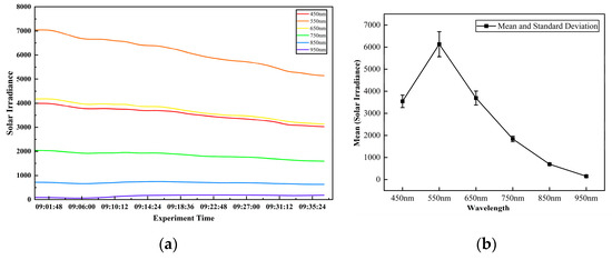
Figure 6.
Solar irradiance and deviation. (a) Solar irradiance changes; (b) mean and standard deviation.
To reflect the effect of random illumination variation on BRDF modeling, we intercepted the same image elements within the same position from the acquired hyperspectral images at different times. We acquired the changes in their DN value curves as shown in Figure 7. It can be seen that there are obvious changes in the DN value curves acquired at the same position before and after 10 min on the 50% target mark, with the largest changes in the DN values between 500 and 800 nm. This variation affects the BRDF quantization research to a great extent, with random and unpredictable effects on the fitting of BRDF models. Therefore, it is crucial to eliminate the random variation of illumination.
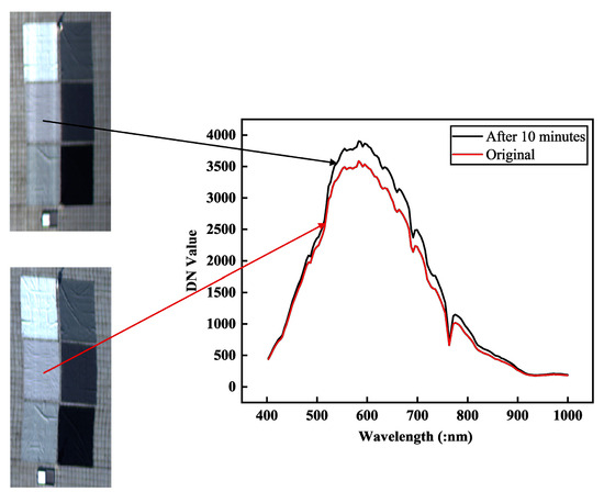
Figure 7.
Change in DN curve after 10 min on the same target.
The hyperspectral imager used in the experiment has a spectral range of 400–1000 nm and contains 150 bands. The acquired hyperspectral images were arranged according to the spatial angle at the acquisition time. The corresponding hyperspectral images under each angular combination were sampled and averaged at multiple points to obtain the reflectance data under the 150 bands. The target area was radiatively corrected by utilizing the acquired target and the standard plate reflectance, and the targets were corrected with each other. The target area was radiometrically fixed using the collected target and standard plate reflectance, and the targets were corrected with each other to obtain the standard reflectance curve under the corresponding spatial angle combination in the target area.
4. Results
4.1. Measured Reflectance Distribution
Multiple-angle information was measured for each target in the test. This section selected 40% of the targets to demonstrate the measured reflectance at 495 nm and 695 nm monochromatic bands (e.g., Figure 8). In Figure 8, the polar diameter indicates the reflectivity magnitude, and the polar angle shows the observation azimuth angle VAA, with the 0° direction being the geographic due north direction and the VAA interval of 30°. The different shaped blocks in red, orange, yellow, and green colors represent the reflectance of the VZA at 5° intervals within 0–20°. The relative errors of the measured data for the 40% target are 6.25% and 6.26% at 495 nm and 695 nm, respectively. The directional distribution of the BRF properties of the same target tends to be consistent in different wavelength bands.
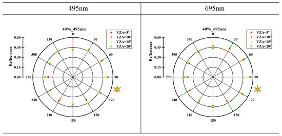
Figure 8.
Measured reflectance of 495 and 695 nm 40% targets.
4.2. Model Fitting Results for Different Bands of the Same Target
In the test, 150 typical bands between 400 nm and 1000 nm were fitted. For demonstration purposes, 40% of the target fitting results at 495 nm and 695 nm were selected in this chapter to compare the fitting results of the three models before and after the improvement.
The fitting results at 495 nm are shown in Figure 9, and those at 695 nm are shown in Figure 10. Figure 9 shows that the three models have a “clustering” effect on the original data, and the BRF shapes fitted by each model are more precise and symmetrically distributed. The difference between the maximum and minimum values narrows, but the three fitting results are slightly higher than the accurate reflectance data. After introducing the illumination correction factor, the BRF distribution of the target is more uniform, which vastly improves the slightly higher fitted values and reduces the error between the fundamental values and the target. From the deviation of the model before and after the improvement, the change of the Kernel model is mainly concentrated in the center of the target, and the shape of the BRF distribution before and after illumination correction changes a lot but still maintains a symmetric distribution.
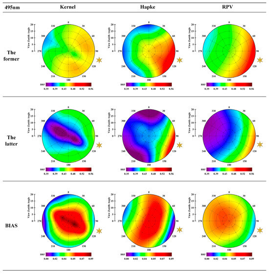
Figure 9.
40% target model fitting and bias before and after illumination correction at 495 nm.
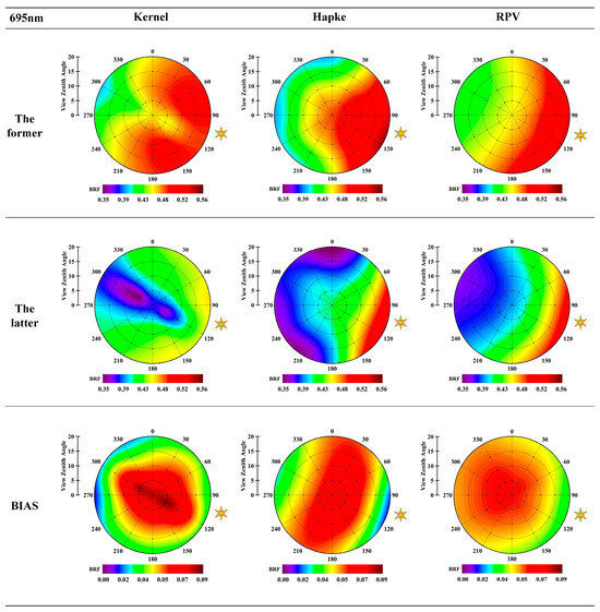
Figure 10.
40% target model fitting and bias before and after illumination correction at 695 nm.
The “RPV” model is the same as the “Hapke” model; the illumination correction does not affect the shape distribution of the BRF, and the range of changes in the “RPV” model has a “region-like” distribution. The fitting results show that the BRF of the target is spatially distributed regionally, and the hotspot effect of the Hapke model and the RPV model is noticeable. After introducing the illumination correction factor, all three models numerically reduced the fitting error significantly compared with the original model, making the fitting results close to the real value of the target.
Figure 10 shows the fitting results of 695 nm data under the 40% target; compared with the 495 nm fitting results, the shape of the BRF is more similar, and the directional distribution is more consistent; the difference mainly focuses on the size of the numerical aspects; the fitting value of 495 nm is more significant, and the fitting value of 695 nm is smaller, which is mainly dependent on the actual collection of the reflectance data. The original model focuses on the reflectance data under the corresponding wavelength only, while the improved model introduces the wavelength term, which can distinguish the BRF distribution between different wavelengths to a more significant extent and link the BRF between different wavelengths. The original model only focuses on the reflectance data at the corresponding wavelengths and is not sensitive to the magnitude of the wavelengths. In contrast, the improved model introduces a wavelength term, which can differentiate the BRF distributions between different wavelengths to a greater extent and can also link the BRFs between different wavelengths.
4.3. Model Fitting Results for Different Targets in the Same Band
For the BRF distribution of targets in typical bands, 20%, 40%, and 50% reflectance targets were selected at 495 nm. The fitting ability and distribution of the results before and after the improvement of the three models were considered. The effect of the observation zenith angle on the accuracy of the models was investigated. The results for fixed observation zenith angles of 5°, 10°, and 15° are shown in Figure 11, where the polar angle indicates the observation azimuth and the polar diameter indicates the reflectance value at the observation azimuth and fixed observation zenith angle. For the same target, the reflectivity factors collected under different observation zenith angles match, indicating that the observation azimuth angle has less influence on the reflectivity of the same target.
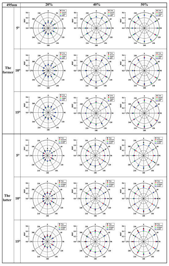
Figure 11.
Multi-gray scale targets fitting results under different observation zenith angles.
In Figure 11, the measured data on 20% of the targets are significant in the observed azimuth angle of 0–90°, small in 180–270°, and “complementary” in the symmetric position in the range of 0–360°, and similar distribution patterns exist in the measured data on 40%, 50%, and the rest of the targets. The three models were fitted to the raw data, and all three models had reasonable constraints on the reflectance factor in the spatial range and could limit the discrete raw data to the neighborhood of the standard data, as shown in Figure 11 (the former). Before the illumination correction factor, the results of the three models were slightly more prominent. Still, the relative deviation between the models is minor, the target spatial reflectance distribution characteristics are apparent, and the three models are numerically more consistent. After the introduction of the illumination correction factor to improve the model, as shown in Figure 11 (The latter), the constraints of the three models on the data still exist; at the 5° observation zenith angle, the kernel model for different reflectance targets is slight, but the degree of smallness will be reduced with the increase of target reflectance. At the 10° zenith angle, the Kernel model fits are significant, but again, the effect is reduced with increasing target emissivity, and the Hapke and RPV models are closer, with the exact location of the hotspot effect. At the 15° zenith angle, the raw data distribution shows that the data quality is higher at this time, and the fitting results of the three models are more consistent in distribution and closer in value.
4.4. Model Fit Coefficients
The Kernel model was fitted to six targets with different reflectivity, and the model’s essential coefficients C(Coefficient) for typical monochromatic bands are shown in Table 3. The anisotropic kernel coefficient, ƒiso, increases with the target reflectivity in all three typical monochromatic bands before the introduction of the illumination change. The body scattering kernel coefficient ƒvol decreases with increasing target reflectivity and increases in absolute value. The geometrical optics kernel ƒgeo improves with increasing target reflectivity. After considering illumination, ƒiso, ƒvol, and ƒgeo of typical monochromatic bands all decrease compared to the previous ones but still tend to change with the increase of target reflectivity.

Table 3.
Kernel coefficient.
The Hapke model is more sensitive to the single-scattering albedo and the hotspot effect, and the single-scattering albedo shows different trends at different wavelengths, as shown in Table 4, with values between 0 and 1. The single-scattering albedo increases gradually from low reflectivity to high reflectivity targets. For the same target, in the typical monochromatic wavelength band, the single scattering albedo changes little and tends to a stable value; in the high reflectivity target, it is more prominent and gradually grows to a saturation value.

Table 4.
Hapke coefficient.
The RPV model was fitted to the data, and its parameters reflect the relative amount of forward and backward scattering. In Table 5, the forward scattering is larger than the backward scattering for different targets in typical monochromatic bands, and the relative amount increases after introducing the light correction factor.

Table 5.
RPV coefficient.
4.5. Effect of Illumination and VZA Variations on Model Accuracy
Figure 12 shows the effect of illumination volatility on model accuracy. Selecting six typical bands of irradiance change values during the test period, it can be seen that the volatility of illumination has an increasing trend between 450 nm and 550 nm, reaches the maximum value at 550 nm, has a decreasing trend after 550 nm, and is stable after 950 nm, but the volatility value of illumination is still considerable before 750 nm. The three models increase the MSE with the increase of illumination volatility. The model error is the largest between 550 nm and 750 nm, and the illumination volatility is also the strongest in the range of the band; 950 nm, and the nearby illumination bands have the most minor change. The model’s accuracy is kept stable but still has a significant error. This is because, for solar illumination, most of the radiant energy is concentrated in the visible part. The actual illumination fluctuations and random changes are mainly focused in this part. The illumination fluctuations in the rest of the band range are insignificant compared to the visible part. At the same time, 950 nm is already located at the end of the hyperspectral camera response; the acquired data is relatively rough, so the model is maintained at a lower and more stable accuracy.

Figure 12.
Impact of illumination variations on model accuracy.
Figure 13 shows the effect of changing the observed zenith angle from 5° to 25° on the model’s accuracy before and after the model improvement. The trend of the model before and after the model improvement is the same; the model error continues to decrease in the range of 5° to 15°, and the model accuracy is highest at the observed zenith angle of 15°. The model error gradually increases in the range of 15° to 25°.

Figure 13.
Impact of VZA on model accuracy.
4.6. Spectral Angle of the Target before and after Model Improvement
Table 6, Table 7 and Table 8 calculate the spectral angles of the model-fitted values and the measured values under typical monochromatic bands after the three model improvements, respectively. Six gray-level targets at 495 nm, 695 nm, and 795 nm maintain smaller spectral angles.

Table 6.
K-Kernel spectral angle.

Table 7.
K-Hapke spectral angle.

Table 8.
K-RPV spectral angle.
5. Discussion
We used a UAV push-broom hyperspectral imaging system to obtain multi-angle information on six gray-scale targets in the target area and synchronously acquired the illumination changes during the experiment. The reflectance distribution characteristics of the raw data, i.e., the problems of uneven data distribution and low quality, are first analyzed, and solutions are given. Three different types of BRDF original and improved models were used for fitting, and the fitting ability of the three models, the sensitivity, and the focus of the model parameters to multi-angle data were analyzed. The reflectance deviations before and after illumination correction are also compared.
In Figure 8, the measured reflectance data of the 40% target under the monochromatic typical bands of 495 nm and 695 nm can be seen as a more obvious symmetrical distribution, with better uniformity and numerically significant values. Still, the distribution of BRF shapes of the 40% target under the two bands tends to be consistent, which is in line with the spatial distribution characteristics of the target. The acquired data strongly support the model fitting, which verifies the use of push-broom hyperspectral imaging for BRDF modeling at the data level.
Figure 9 and Figure 10 show that the data fitted to 40% of the target at 495 and 695 nm. The three original models can constrain the distribution of target BRFs smoothly and uniformly, but the model-fitted data have the problem of large fitted values. After introducing the illumination correction factor (the latter), the improved model retains the characteristics of the previous uniformity distribution but reduces the BRF value to be closer to the target’s real value. The reason for this is that the measured data, due to illumination variations and noise, affects the fitting effect of the model and makes it difficult to highlight the BRF characteristics of the target. Under different wavelength bands, the BRF shapes of 40% of targets fitted by the improved model converge under 495 nm and 695 nm, and the changes are mainly manifested in the slight differences in the numerical values. From the fitting effect of each model, the fitting value of the Kernel model is on the large side, and the shape of BRF before and after illumination improvement is more different. The Hapke model can fully describe the distribution of surface properties of the target, so it can reflect the influence of scattering on the distribution of BRF and highlight the hotspot effect. The RPV model can consider the hotspot effect and backward and forward scattering, and the results have the details of the Hapke model and the uniformity of the Kernel model. The improvement effects of the three BRDF models demonstrate the applicability of the proposed illumination correction factors to different models.
In Figure 11, the distribution of the measured reflectivity factors of the 20%, 40%, and 50% targets at 5°, 10°, and 15° observation zenith angles are not uniform, and there are differences with the real data of the targets. The reasons for this are analyzed as systematic errors caused by the radiometric calibration and UAV system acquisition process and the influence of illumination changes on the measured data. When enough data are collected, the systematic error can be reduced or eliminated by multiple iterations of the model, and illumination variations can be eliminated by improving the model. In terms of BRF values, after introducing the illumination correction factor to improve the model, the fitting error of the model is substantially reduced, and the numerical deviation of the target BRF is diminished. The results of the three grayscale targets and three VZAs demonstrate that the proposed improved model is robust to different reflectance and observation angles and can increase its ability to resist multiple influencing factors while retaining the fitting characteristics of the original model.
The BRF fitting results and representative parameters for the six targets before and after the model improvement are shown in Table 3, Table 4 and Table 5, which show that the illumination correction factor is real and effective for the model improvement, and it reduces the uncertainty effects of random illumination changes on the model parameters. The original model itself can improve the inversion accuracy of the parameters contained in the model.
In Figure 12 and Figure 13, the effect of illumination and VZA changes on the model accuracy can be seen as a trend of increasing or decreasing illumination volatility, with a subsequent increase or decrease in model error. After illumination correction, the model shows higher accuracy under different VZA; the best VZA is 15°. For the optimal observation angle, we believe that it is related to the surface characteristics of the target as well as the position of the target in the imaging space; specifically, features made of different materials, when imaged at different positions in space, will show better reflections at certain angles. Table 6, Table 7 and Table 8 reflect the stability of the improved model in the spectral dimension for the same target, which can eliminate the effect of illumination on the target’s BRF characteristics while preserving the target’s spectral characteristics.
The illumination correction factor proposed in this paper can eliminate the illumination variations to the maximum extent. We calculated the RMSE of the three models before and after the improvement, as shown in Table 9, Table 10 and Table 11. From the results, the three improved models significantly improved the accuracy of different targets and bands. In the actual BRDF modeling, the illumination is unchanged, or the irradiance change in a particular band is smooth; the improved model can be degraded to the original BRDF model, and the illumination changes are significant and more random; the enhanced model is able to eliminate this effect, and the larger the fluctuation and the more random the changes are, the more the improved model advantages are manifested. The model has obvious superiority in various illumination environments and all bands. This is significant for exploring the model’s potential and promoting its application.

Table 9.
BRF fitting errors of the Kernel model for multiple targets and bands before and after illumination correction.

Table 10.
BRF fitting errors of the Hapke model for multiple targets and bands before and after illumination correction.

Table 11.
BRF fitting errors of the RPV model for multiple targets and bands before and after illumination correction.
6. Conclusions
To solve the problem of UAV-carried push-broom hyperspectral BRDF being challenging to acquire and model, the random variation of outdoor illumination affects the accuracy of BRDF modeling. In this paper, we propose a rapid multi-angle information acquisition scheme and BRDF modeling method considering outdoor illumination variations, which solves the problem of difficulty in acquiring and modeling UAV-carried push-broom hyperspectral BRDFs and incorporates illumination variations into the BRDF model, which solves the problem of illumination affecting the actual modeling accuracy of the BRDF model. This lightweight system can quickly acquire multi-angle reflectance information under different wavelength bands required for BRDF modeling in the target area. It can obtain solar illumination changes in real-time. We propose a light correction factor by combining the effect of illumination changes on the BRDF model and using this factor to improve the three traditional BRDF models. The improved model can eliminate the effect of illumination changes on the accuracy of BRDF modeling. Multi-target BRDF modeling was completed using this set of schemes and methods. The errors before and after model improvement were verified on targets with different gray levels. The potential of push-broom hyperspectral imagers at the data level of BRDF modeling was explored to demonstrate the feasibility and applicability of the modeling. Our next goal is to continue to improve the multi-angle information acquisition system, further optimize the matching scheme of the data acquired by the multi-mode equipment, gain multi-angle information based on single-pixel accuracy, fully consider the spatial factors affecting the model accuracy, and continue to explore the model’s upgradability and generalizability, to achieve fast BRDF modeling with high accuracy and high spectra and in a wide range.
Author Contributions
Conceptualization, Z.W. and H.L.; methodology, Z.W. and H.L.; validation, Z.W., L.S. and J.C.; investigation, Z.W.; writing—original draft preparation, Z.W.; writing—review and editing, Z.W., H.L. and S.W.; project administration, H.L.; funding acquisition, H.L. and S.W. All authors have read and agreed to the published version of the manuscript.
Funding
This work was supported in part by the National Key Research and Development Program of China (No. 2022YFF1300201 and 2021YFD2000100) and in part by the National Natural Science Foundation of China (No. 42101380 and 42176182).
Data Availability Statement
The data presented in this study are available on request from the corresponding author. The data are not publicly available due to private.
Conflicts of Interest
The authors declare no conflicts.
References
- Zhang, H.; Jiao, Z.T.; Dong, Y.D.; Li, J.Y.; Li, X.W. Albedo retrieved from BRDF archetype and surface directional reflectance. J. Remote Sens. 2015, 19, 355–367. [Google Scholar] [CrossRef]
- Zhu, W.; You, D.; Wen, J.; Tang, Y.; Gong, B.; Han, Y. Evaluation of Linear Kernel-Driven BRDF Models over Snow-Free Rugged Terrain. Remote Sens. 2023, 15, 786. [Google Scholar] [CrossRef]
- Wierzbicki, D.; Kedzierski, M.; Fryskowska, A.; Jasinski, J. Quality Assessment of the Bidirectional Reflectance Distribution Function for NIR Imagery Sequences from UAV. Remote Sens. 2018, 10, 1348. [Google Scholar] [CrossRef]
- Han, Y.; Wen, J.; Xiao, Q.; Bao, Y.; Chen, X.; Liu, Q.; He, M. Review of the Land Surface BRDF Inversion Methods Based on Remotely Sensed Satellite Data. Natl. Remote Sens. Bull. 2023, 27, 2024–2040. [Google Scholar] [CrossRef]
- Zhang, H.; Jiao, Z.; Chen, L.; Dong, Y.; Zhang, X.; Lian, Y.; Qian, D.; Cui, T. Quantifying the Reflectance Anisotropy Effect on Albedo Retrieval from Remotely Sensed Observations Using Archetypal BRDFs. Remote Sens. 2018, 10, 1628. [Google Scholar] [CrossRef]
- Zhen, Z.; Chen, S.; Yin, T.; Gastellu-Etchegorry, J.-P. Improving Crop Mapping by Using Bidirectional Reflectance Distribution Function (BRDF) Signatures with Google Earth Engine. Remote Sens. 2023, 15, 2761. [Google Scholar] [CrossRef]
- Yao, C.; Sun, Z.; Lu, S. Reducing BRDF Effects on the Estimation of Leaf Biochemical Parameters Using the Nonpolarized Reflectance Factor in the Hemispheric Space. IEEE Trans. Geosci. Remote Sens. 2022, 60, 1–17. [Google Scholar] [CrossRef]
- Han, W.; Lim, J.; Lee, S.-J.; Kim, C.-Y. Reducing BRDF Effects on the Estimation of Leaf Biochemical Parameters Using the Nonpolarized Reflectance Factor in the Hemispheric SpaceDistribution Function (BRDF)-Based Coarseness Prediction of Textured Metal Surface. IEEE Access 2022, 10, 32461–32469. [Google Scholar] [CrossRef]
- Zhong, Y.; Wang, X.; Xu, Y.; Wang, S.; Jia, T.; Hu, X.; Zhao, J.; Wei, L.; Zhang, L. Mini-UAV-Borne Hyperspectral Remote Sensing: From Observation and Processing to Applications. IEEE Geosci. Remote Sens. Mag. 2018, 6, 46–62. [Google Scholar] [CrossRef]
- Zhang, C.B.; Yang, S.T.; Zhao, C.S.; Lou, H.Z.; Zhang, Y.C.; Bai, J.; Wang, Z.W.; Guan, Y.B.; Zhang, Y. Topographic data accuracy verification of small consumer UAV. J. Remote Sens. 2018, 22, 185–195. [Google Scholar] [CrossRef]
- Tao, B.C.; Hu, X.Q.; Yang, L.K.; Zhang, L.; Chen, L.; Xu, N.; Wang, L.; Wu, R.Q.; Zhang, D.F.; Zhang, P. BRDF feature observation method and modeling of desert site based on UAV platform. Natl. Remote Sens. Bull. 2021, 25, 1964–1977. [Google Scholar] [CrossRef]
- Song, L.; Li, H.; Chen, T.; Chen, J.; Liu, S.; Fan, J.; Wang, Q. An Integrated Solution of UAV Push-Broom Hyperspectral System Based on Geometric Correction with MSI and Radiation Correction Considering Outdoor Illumination Variation. Remote Sens. 2022, 14, 6267. [Google Scholar] [CrossRef]
- Zhang, H.; Zhang, B.; Wei, Z.; Wang, C.; Huang, Q. Lightweight Integrated Solution for a UAV-Borne Hyperspectral Imaging System. Remote Sens. 2020, 12, 657. [Google Scholar] [CrossRef]
- Shi, Y.; Fu, B.; Wang, N.; Chen, Y.; Fang, J. Multispectral Image Quality Improvement Based on Global Iterative Fusion Constrained by Meteorological Factors. Cogn. Comput. 2023, 16, 1–21. [Google Scholar] [CrossRef]
- Chang, Y.X.; Jiao, Z.T.; Dong, Y.D.; Zhang, X.N.; He, D.D.; Yin, S.Y.; Cui, L.; Ding, A.X. Parameterization and correction of hotspot parameters of Ross-Li kernel driven models on POLDER dataset. J. Remote Sens. 2019, 23, 661–672. [Google Scholar] [CrossRef]
- Dong, Y.D.; Jiao, Z.T.; Zhang, H.; Li, J.Y.; Jiao, G.P.; Shi, H.Y. Efficient algorithm for improving the hotspot effect of the operational MODIS BRDF product. J. Remote Sens. 2014, 18, 804–825. [Google Scholar] [CrossRef]
- Guo, J.; Jiao, Z.T.; Ding, A.X.; Dong, Y.D.; Zhang, X.N.; Cui, L.; Yin, S.Y.; Chang, Y.X.; Xie, R. Evaluation of three BRDF models’ performance using spaceborne POLDER snow data. Natl. Remote Sens. Bull. 2022, 26, 2060–2072. [Google Scholar] [CrossRef]
- Li, J.; Jiao, Z.; Zhang, H.; Dong, Y. Variance of bidirectional reflectance and its application using operational MODIS BRDF model. J. Remote Sens. 2015, 19, 750–760. [Google Scholar] [CrossRef]
- Qiu, F.; Huo, J.W.; Zhang, Q.; Chen, X.H.; Zhang, Y.G. Observation and analysis of bidirectional and hotspot reflectance of conifer forest canopies with a multiangle hyperspectral UAV imaging platform. Natl. Remote Sens. Bull. 2021, 25, 1013–1024. [Google Scholar] [CrossRef]
- Wang, L.; Hu, X.Q.; Xu, N.; Chen, L.; Zhang, P.; Xu, H.L. Research on Construction of directional reflectance reference Model for Desert Stable Earth Targets. Natl. Remote Sens. Bull. 2023, 27, 2270–2282. [Google Scholar] [CrossRef]
- Mamaghania, B.G.; Salvaggioa, C. Comparative study of panel and panelless-based reflectance conversion techniques for agricultural remote sensing. arXiv 2019, arXiv:1910.03734. [Google Scholar]
- Burkart, A.; Cogliati, S.; Schickling, A.; Rascher, U. A Novel UAV-Based Ultra-Light Weight Spectrometer for Field Spectroscopy. IEEE Sens. J. 2014, 14, 62–67. [Google Scholar] [CrossRef]
- Schneider-Zapp, K.; Cubero-Castan, M.; Shi, D.; Strecha, C. A new method to determine multi-angular reflectance factor from lightweight multispectral cameras with sky sensor in a target-less workflow applicable to UAV. Remote Sens. Environ. 2019, 229, 60–68. [Google Scholar] [CrossRef]
- Franch, B.; Vermote, E.; Skakun, S.; Roger, J.-C.; Masek, J.; Ju, J.; Villaescusa-Nadal, J.L.; Santamaria-Artigas, A. A Method for Landsat and Sentinel 2 (HLS) BRDF Normalization. Remote Sens. 2019, 11, 632. [Google Scholar] [CrossRef]
- Han, J.; Tao, Z.; Xie, Y.; Li, H.; Yi, H.; Guan, X. Validation of the TOA Products of the Baotou Sandy Site With Landsat8/OLI Considering BRDF Correction. IEEE Trans. Geosci. Remote Sens. 2023, 61, 1–11. [Google Scholar] [CrossRef]
- Jia, W.; Pang, Y.; Tortini, R.; Schläpfer, D.; Li, Z.; Roujean, J.-L. A Kernel-Driven BRDF Approach to Correct Airborne Hyperspectral Imagery over Forested Areas with Rugged Topography. Remote Sens. 2020, 12, 432. [Google Scholar] [CrossRef]
- Tan, Y.; Li, X.; Yang, X.; Jin, Y. Research and Analysis on the Angles Normalization of the Domestic GF-1 Satellite Based on MODIS BRDF Products. In Proceedings of the 2022 3rd International Conference on Geology, Mapping and Remote Sensing (ICGMRS), Zhoushan, China, 22–24 April 2022; pp. 565–573. [Google Scholar]
- Cheng, J.; Wen, J.; Xiao, Q.; Hao, D.; Lin, X.; Liu, Q. Exploring the Applicability of the Semi-Empirical BRDF Models at Different Scales Using Airborne Multi-Angular Observations. IEEE Geosci. Remote Sens. Lett. 2022, 19, 1–5. [Google Scholar] [CrossRef]
- Ye, L.; Xiao, P.; Zhang, X.; Feng, X.; Hu, R.; Ma, W.; Li, H.; Song, Y.; Ma, T. Evaluating Snow Bidirectional Reflectance of Models Using Multiangle Remote Sensing Data and Field Measurements. IEEE Geosci. Remote Sens. Lett. 2022, 19, 1–5. [Google Scholar] [CrossRef]
- Jiao, Z.; Ding, A.; Kokhanovsky, A.; Schaaf, C.; Bréon, F.-M.; Dong, Y.; Wang, Z.; Liu, Y.; Zhang, X.; Yin, S.; et al. Development of a snow kernel to better model the anisotropic reflectance of pure snow in a kernel-driven BRDF model framework. Remote Sens. Environ. 2019, 221, 198–209. [Google Scholar] [CrossRef]
- Yan, K.; Li, H.; Song, W.; Tong, Y.; Hao, D.; Zeng, Y.; Mu, X.; Yan, G.; Fang, Y.; Myneni, R.B.; et al. Extending a Linear Kernel-Driven BRDF Model to Realistically Simulate Reflectance Anisotropy Over Rugged Terrain. IEEE Trans. Geosci. Remote Sens. 2022, 60, 1–16. [Google Scholar] [CrossRef]
- Zhang, Y.; Zhang, W.; Chen, Z.; Li, H. Influence of Channel Center Wavelength Shift of the Hyperspectral Remote Sensor on Red Edge Spectra. Acta Opt. Sin. 2021, 41, 1428003. [Google Scholar]
Disclaimer/Publisher’s Note: The statements, opinions and data contained in all publications are solely those of the individual author(s) and contributor(s) and not of MDPI and/or the editor(s). MDPI and/or the editor(s) disclaim responsibility for any injury to people or property resulting from any ideas, methods, instructions or products referred to in the content. |
© 2024 by the authors. Licensee MDPI, Basel, Switzerland. This article is an open access article distributed under the terms and conditions of the Creative Commons Attribution (CC BY) license (https://creativecommons.org/licenses/by/4.0/).