
Unified Interpretable Deep Network for Joint Super-Resolution and Pansharpening


Abstract
1. Introduction
- -
- To the best of our knowledge, we are the first to build a new model to formulate the SR and pansharpening objective in a unified optimization problem, which is convenient for effectively preserving spatial as well as spectral resolution. In addition, two deep priors about the latent distributions of the latent high-resolution multispectral images are adopted to improve the accuracy of the model.
- -
- To solve this model efficiently, we construct UIJSP-Net by utilizing the unfolding technology based on some iterative steps derived from the ADMM.
- -
- Then we validate this method in both simulated and real datasets, proving its advantage over other state-of-the-art methods.
2. Related Work
2.1. SR
2.2. Pansharpening
3. Proposed Method
3.1. Formulation of the Proposed JSP Model
3.2. Solution to the Proposed JSP Model
| Algorithm 1: Proposed JSP algorithm. |
| Input , , , , , , , (maximum number of iterations), , , , , For to do Update in the closed-form from Equations (7), (10), and (11). Update in the closed-form from Equation (13). Update in the closed-form from Equation (14). End Output . |
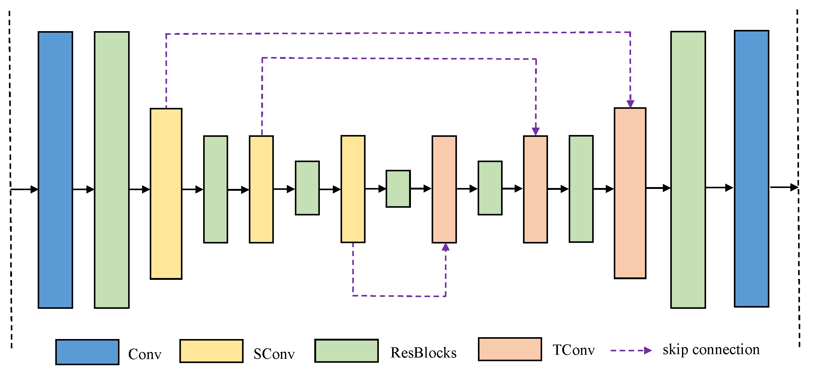
3.3. Network Design
4. Experimental Results
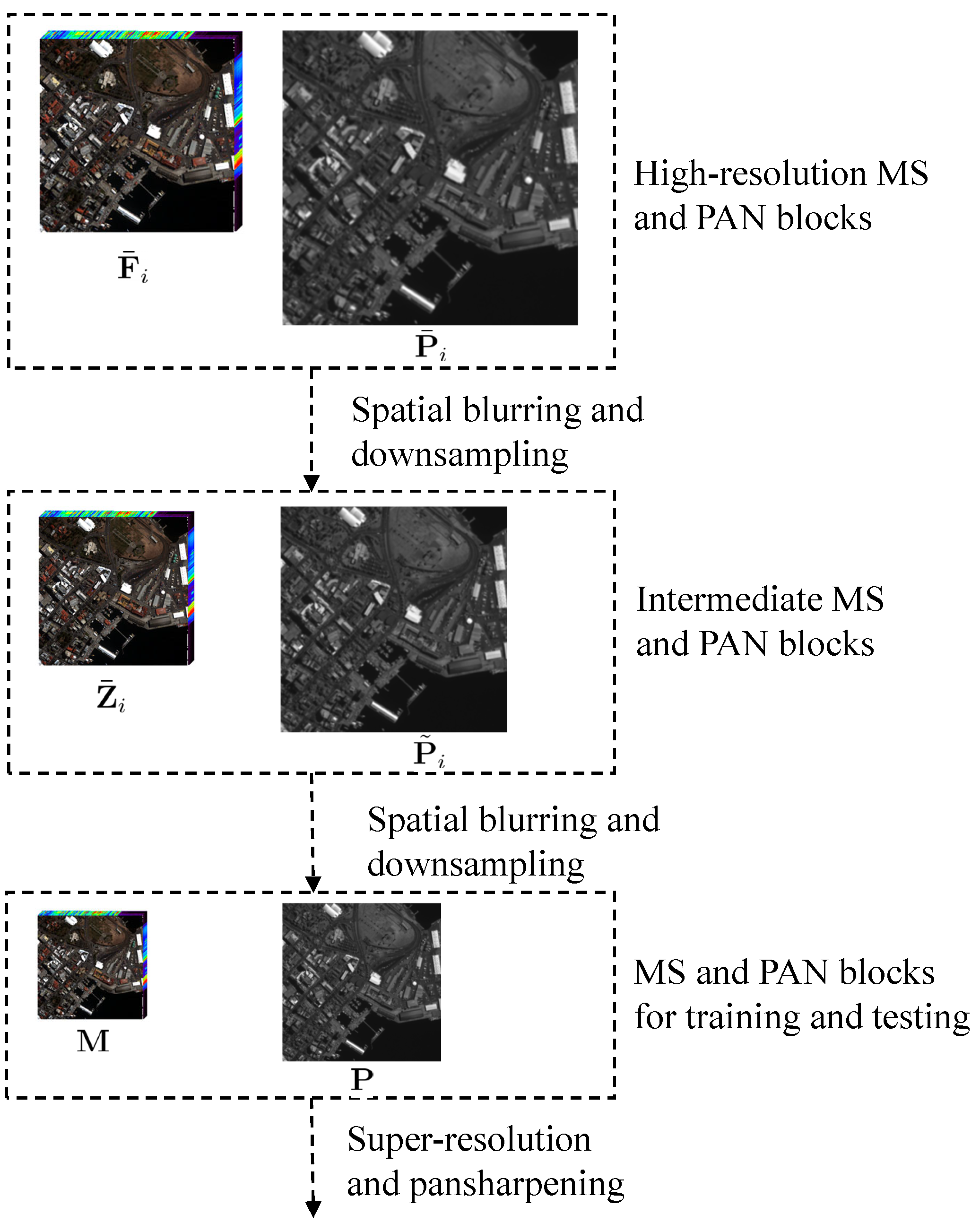
4.1. Experimental Setting
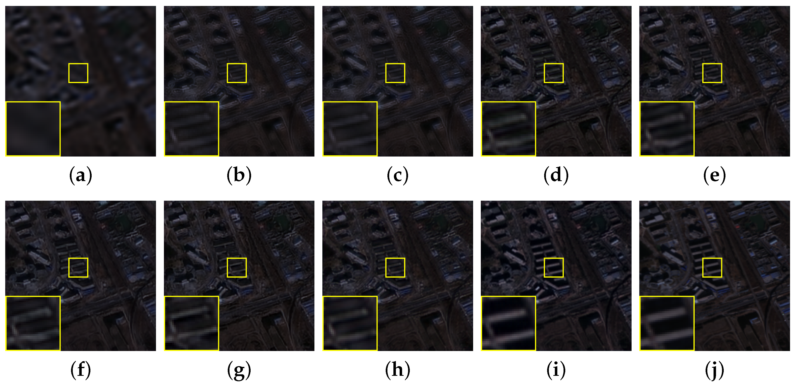
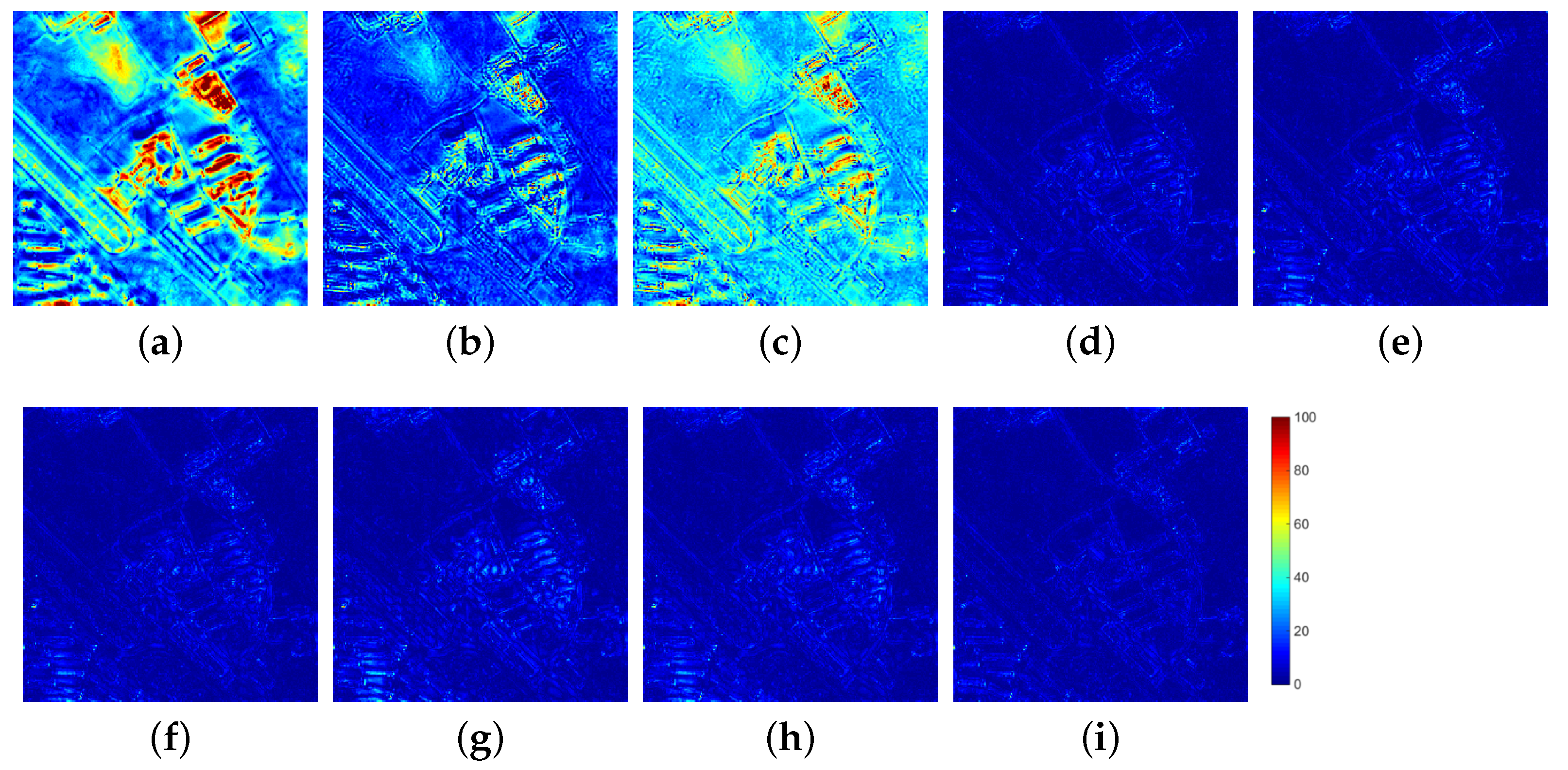
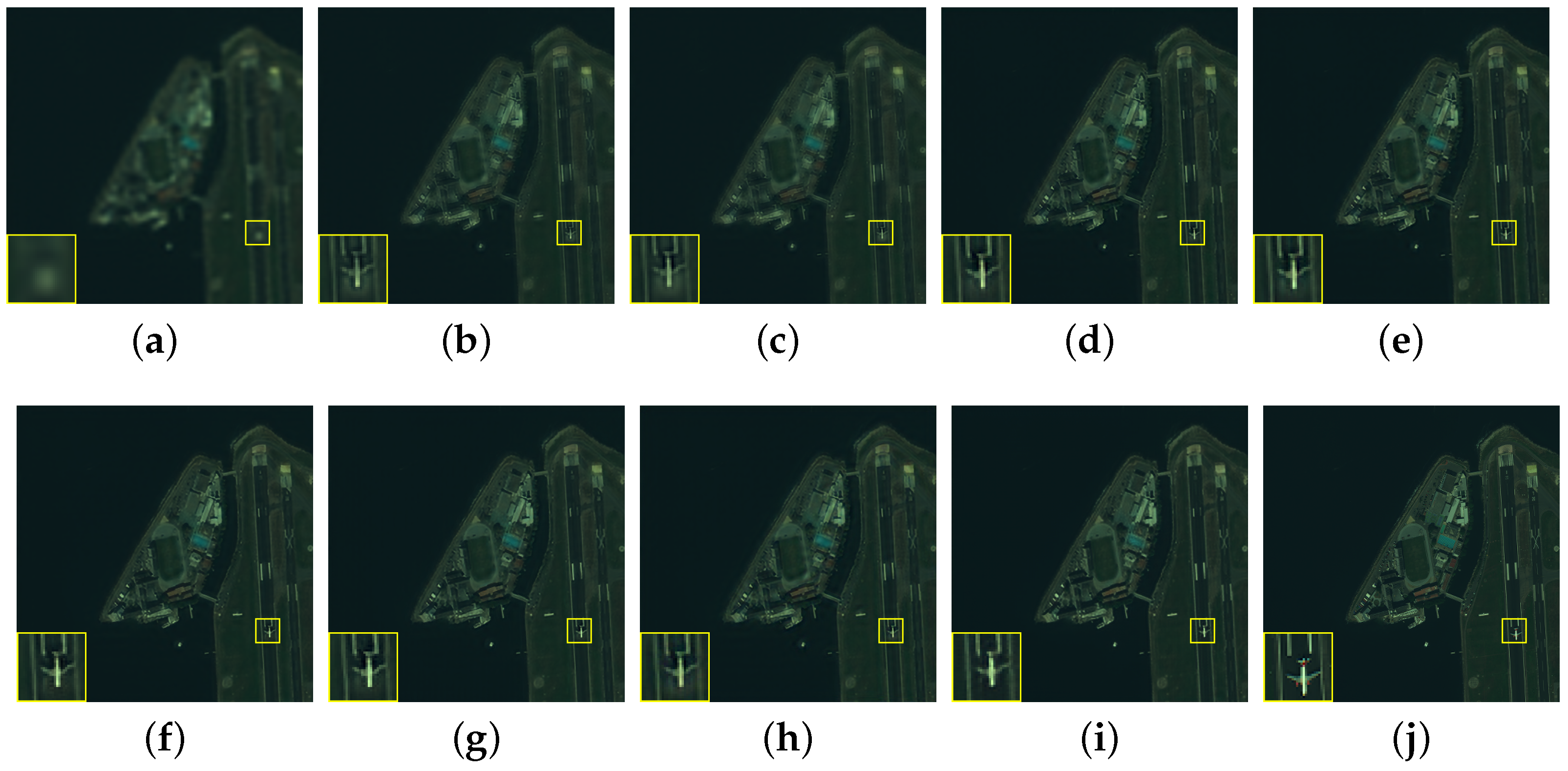
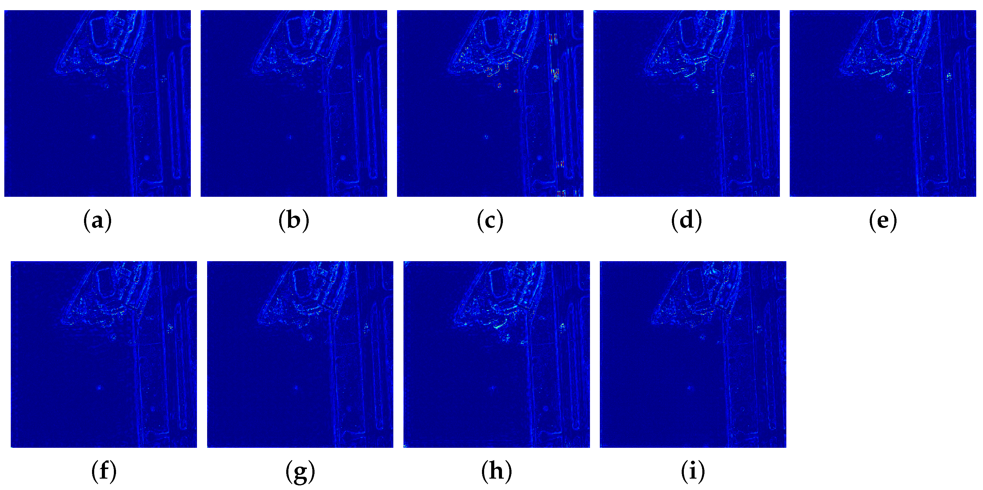
4.2. Simulation Experiments
4.2.1. GaoFen-2 Dataset
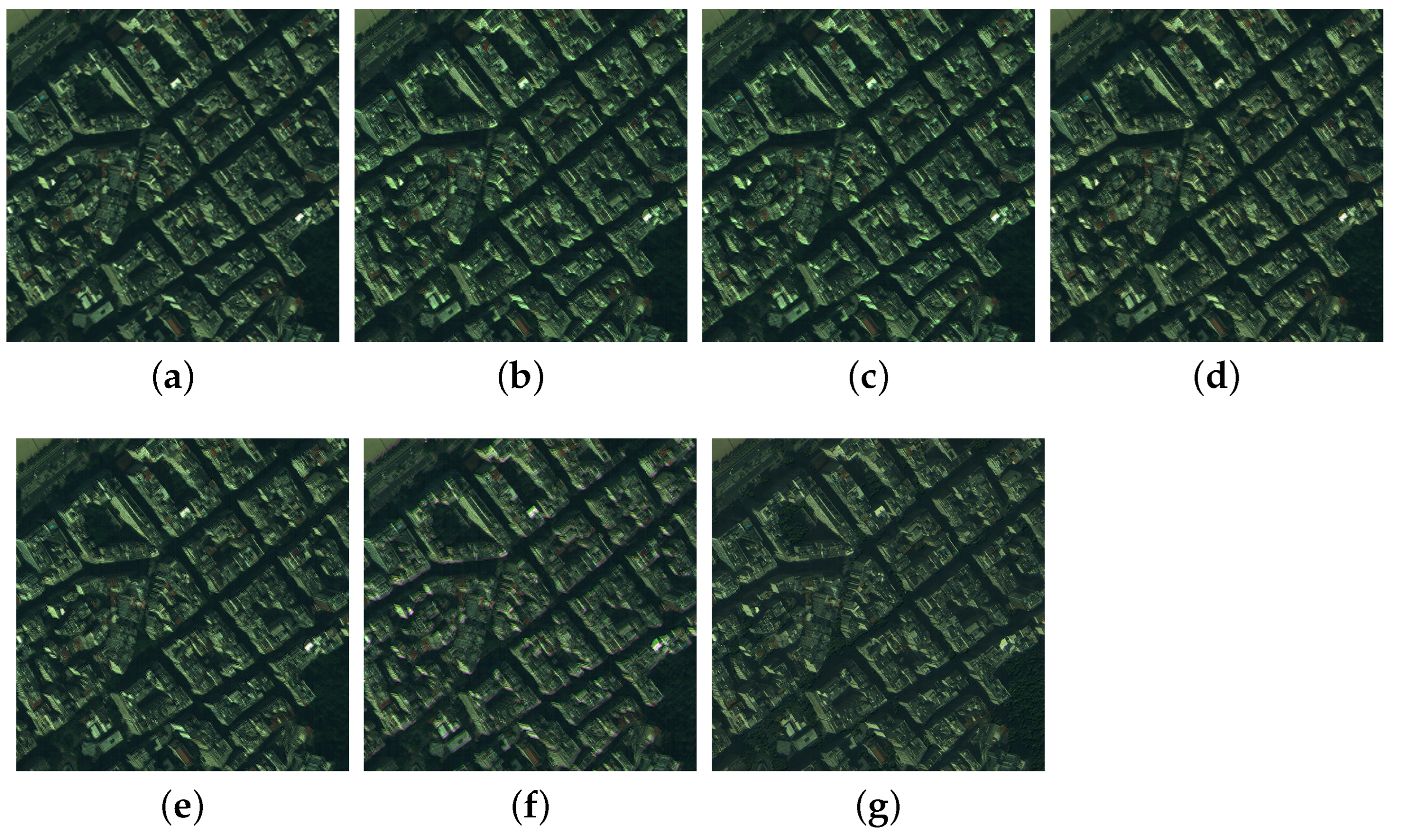
4.2.2. QuickBird Dataset
4.2.3. WorldView-3 Dataset
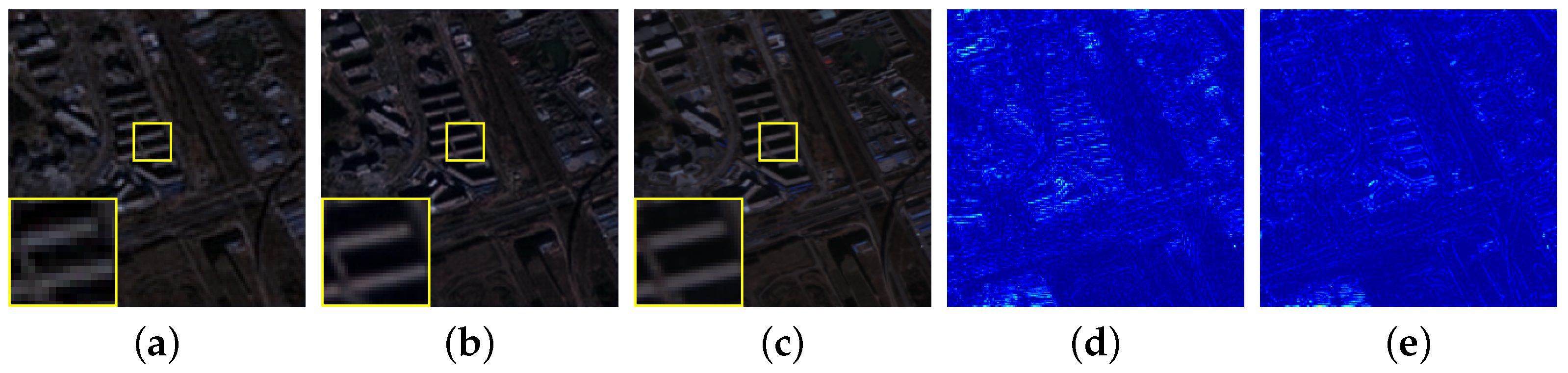
4.3. Real Experiment
4.4. Analysis of Computational Efficiency
4.5. Ablation Study
4.6. NDVI Experiment
5. Conclusions
Author Contributions
Funding
Data Availability Statement
Acknowledgments
Conflicts of Interest
References
- Zhang, T.J.; Deng, L.J.; Huang, T.Z.; Chanussot, J.; Vivone, G. A Triple-Double Convolutional Neural Network for Panchromatic Sharpening. IEEE Trans. Neural Netw. Learn. Syst. 2023, 34, 9088–9101. [Google Scholar] [CrossRef]
- Zhang, M.; Li, S.; Yu, F.; Tian, X. Image fusion employing adaptive spectral-spatial gradient sparse regularization in UAV remote sensing. Signal Process. 2020, 170, 107434. [Google Scholar] [CrossRef]
- Tian, X.; Zhang, W.; Yu, D.; Ma, J. Sparse Tensor Prior for Hyperspectral, Multispectral, and Panchromatic Image Fusion. IEEE/CAA J. Autom. Sin. 2023, 10, 284–286. [Google Scholar] [CrossRef]
- Wang, W.; Zhou, Z.; Zhang, X.; Lv, T.; Liu, H.; Liang, L. DiTBN: Detail Injection-Based Two-Branch Network for Pansharpening of Remote Sensing Images. Remote Sens. 2022, 14, 6120. [Google Scholar] [CrossRef]
- Masi, G.; Cozzolino, D.; Verdoliva, L.; Scarpa, G. Pansharpening by convolutional neural networks. Remote Sens. 2016, 8, 594. [Google Scholar] [CrossRef]
- Yang, J.; Fu, X.; Hu, Y.; Huang, Y.; Ding, X.; Paisley, J. PanNet: A deep network architecture for pan-sharpening. In Proceedings of the IEEE International Conference on Computer Vision, Venice, Italy, 22–29 October 2017; pp. 5449–5457. [Google Scholar]
- Yuan, Q.; Wei, Y.; Meng, X.; Shen, H.; Zhang, L. A multiscale and multidepth convolutional neural network for remote sensing imagery pan-sharpening. IEEE J. Sel. Top. Appl. Earth Obs. Remote Sens. 2018, 11, 978–989. [Google Scholar] [CrossRef]
- Jin, C.; Deng, L.J.; Huang, T.Z.; Vivone, G. Laplacian pyramid networks: A new approach for multispectral pansharpening. Inf. Fusion 2022, 78, 158–170. [Google Scholar] [CrossRef]
- Ke, C.; Liang, H.; Li, D.; Tian, X. High-Frequency Transformer Network Based on Window Cross-Attention for Pansharpening. In Proceedings of the IEEE International Conference on Acoustics, Speech and Signal Processing, Rhodes Island, Greece, 4–10 June 2023; pp. 1–5. [Google Scholar]
- Ma, J.; Yu, W.; Chen, C.; Liang, P.; Guo, X.; Jiang, J. Pan-GAN: An unsupervised pan-sharpening method for remote sensing image fusion. Inf. Fusion 2020, 62, 110–120. [Google Scholar] [CrossRef]
- Chouteau, F.; Gabet, L.; Fraisse, R.; Bonfort, T.; Harnoufi, B.; Greiner, V.; Le Goff, M.; Ortner, M.; Paveau, V. Joint Super-Resolution and Image Restoration for PLÉIADES NEO Imagery. Int. Arch. Photogramm. Remote Sens. Spat. Inf. Sci. 2022, 43, 9–15. [Google Scholar] [CrossRef]
- Zhu, S.; Zeng, B.; Zeng, L.; Gabbouj, M. Image interpolation based on non-local geometric similarities and directional gradients. IEEE Trans. Multimed. 2016, 18, 1707–1719. [Google Scholar] [CrossRef]
- Yang, J.; Wright, J.; Huang, T.; Ma, Y. Image super-resolution as sparse representation of raw image patches. In Proceedings of the IEEE Conference on Computer Vision and Pattern Recognition, Anchorage, AK, USA, 23–28 June 2008; pp. 1–8. [Google Scholar]
- Zhang, K.; Gao, X.; Tao, D.; Li, X. Multi-scale dictionary for single image super-resolution. In Proceedings of the IEEE Conference on Computer Vision and Pattern Recognition, Providence, RI, USA, 16–21 June 2012; pp. 1114–1121. [Google Scholar]
- Freedman, G.; Fattal, R. Image and video upscaling from local self-examples. ACM Trans. Graph. (TOG) 2011, 30, 1–11. [Google Scholar] [CrossRef]
- Dong, C.; Loy, C.C.; He, K.; Tang, X. Learning a deep convolutional network for image super-resolution. In Proceedings of the European Conference on Computer Vision, Zurich, Switzerland, 6–12 September 2014; Springer: Berlin/Heidelberg, Germany, 2014; pp. 184–199. [Google Scholar]
- Dai, T.; Cai, J.; Zhang, Y.; Xia, S.T.; Zhang, L. Second-order attention network for single image super-resolution. In Proceedings of the IEEE Conference on Computer Vision and Pattern Recognition, Long Beach, CA, USA, 15–20 June 2019; pp. 11065–11074. [Google Scholar]
- Zhang, K.; Gool, L.V.; Timofte, R. Deep unfolding network for image super-resolution. In Proceedings of the IEEE Conference on Computer Vision and Pattern Recognition, Seattle, WA, USA, 14–19 June 2020; pp. 3217–3226. [Google Scholar]
- Zhang, Y.; Wei, D.; Qin, C.; Wang, H.; Pfister, H.; Fu, Y. Context reasoning attention network for image super-resolution. In Proceedings of the IEEE International Conference on Computer Vision, Montreal, BC, Canada, 11–17 October 2021; pp. 4278–4287. [Google Scholar]
- Gao, S.; Zhuang, X. Bayesian image super-resolution with deep modeling of image statistics. IEEE Trans. Pattern Anal. Mach. Intell. 2022, 45, 1405–1423. [Google Scholar] [CrossRef]
- Zhou, Z.; Ma, N.; Li, Y.; Yang, P.; Zhang, P.; Li, Y. Variational PCA fusion for Pan-sharpening very high resolution imagery. Sci. China Inf. Sci. 2014, 57, 1–10. [Google Scholar] [CrossRef]
- Aiazzi, B.; Baronti, S.; Selva, M. Improving component substitution pansharpening through multivariate regression of MS + Pan data. IEEE Trans. Geosci. Remote Sens. 2007, 45, 3230–3239. [Google Scholar] [CrossRef]
- Rahmani, S.; Strait, M.; Merkurjev, D.; Moeller, M.; Wittman, T. An adaptive IHS pan-sharpening method. IEEE Geosci. Remote Sens. Lett. 2010, 7, 746–750. [Google Scholar] [CrossRef]
- Liu, J. Smoothing filter-based intensity modulation: A spectral preserve image fusion technique for improving spatial details. Int. J. Remote Sens. 2000, 21, 3461–3472. [Google Scholar] [CrossRef]
- Vivone, G.; Restaino, R.; Dalla Mura, M.; Licciardi, G.; Chanussot, J. Contrast and error-based fusion schemes for multispectral image pansharpening. IEEE Geosci. Remote Sens. Lett. 2013, 11, 930–934. [Google Scholar] [CrossRef]
- Addesso, P.; Restaino, R.; Vivone, G. An Improved Version of the Generalized Laplacian Pyramid Algorithm for Pansharpening. Remote Sens. 2021, 13, 3386. [Google Scholar] [CrossRef]
- Alparone, L.; Garzelli, A.; Vivone, G. Intersensor statistical matching for pansharpening: Theoretical issues and practical solutions. IEEE Trans. Geosci. Remote Sens. 2017, 55, 4682–4695. [Google Scholar] [CrossRef]
- Liu, J.; Liang, S. Pan-sharpening using a guided filter. Int. J. Remote Sens. 2016, 37, 1777–1800. [Google Scholar] [CrossRef]
- Ballester, C.; Caselles, V.; Igual, L.; Verdera, J.; Rougé, B. A variational model for P+ XS image fusion. Int. J. Comput. Vis. 2006, 69, 43–58. [Google Scholar] [CrossRef]
- Palsson, F.; Sveinsson, J.R.; Ulfarsson, M.O. A new pansharpening algorithm based on total variation. IEEE Geosci. Remote Sens. Lett. 2013, 11, 318–322. [Google Scholar] [CrossRef]
- Fu, X.; Lin, Z.; Huang, Y.; Ding, X. A variational pan-sharpening with local gradient constraints. In Proceedings of the IEEE/CVF Conference on Computer Vision and Pattern Recognition, Long Beach, CA, USA, 15–20 June 2019; pp. 10265–10274. [Google Scholar]
- Tian, X.; Chen, Y.; Yang, C.; Ma, J. Variational pansharpening by exploiting cartoon-texture similarities. IEEE Trans. Geosci. Remote Sens. 2021, 60, 1–16. [Google Scholar] [CrossRef]
- Xu, H.; Le, Z.; Huang, J.; Ma, J. A Cross-Direction and Progressive Network for Pan-Sharpening. Remote Sens. 2021, 13, 3045. [Google Scholar] [CrossRef]
- Wei, Y.; Yuan, Q.; Shen, H.; Zhang, L. Boosting the accuracy of multispectral image pansharpening by learning a deep residual network. IEEE Geosci. Remote Sens. Lett. 2017, 14, 1795–1799. [Google Scholar] [CrossRef]
- Zhang, Y.; Liu, C.; Sun, M.; Ou, Y. Pan-sharpening using an efficient bidirectional pyramid network. IEEE Trans. Geosci. Remote Sens. 2019, 57, 5549–5563. [Google Scholar] [CrossRef]
- Deng, L.J.; Vivone, G.; Jin, C.; Chanussot, J. Detail injection-based deep convolutional neural networks for pansharpening. IEEE Trans. Geosci. Remote Sens. 2021, 59, 6995–7010. [Google Scholar] [CrossRef]
- Tian, X.; Li, K.; Wang, Z.; Ma, J. VP-Net: An interpretable deep network for variational pansharpening. IEEE Trans. Geosci. Remote Sens. 2021, 60, 1–16. [Google Scholar] [CrossRef]
- Wen, R.; Deng, L.J.; Wu, Z.C.; Wu, X.; Vivone, G. A novel spatial fidelity with learnable nonlinear mapping for panchromatic sharpening. IEEE Trans. Geosci. Remote Sens. 2023, 61, 5401915. [Google Scholar] [CrossRef]
- Zhou, M.; Huang, J.; Fang, Y.; Fu, X.; Liu, A. Pan-sharpening with customized transformer and invertible neural network. In Proceedings of the AAAI Conference on Artificial Intelligence, Washington, DC, USA, 7–14 February 2022; Volume 36, pp. 3553–3561. [Google Scholar]
- Beck, A.; Teboulle, M. A fast iterative shrinkage-thresholding algorithm for linear inverse problems. SIAM J. Imaging Sci. 2009, 2, 183–202. [Google Scholar] [CrossRef]
- Zhang, K.; Li, Y.; Zuo, W.; Zhang, L.; Van Gool, L.; Timofte, R. Plug-and-Play Image Restoration With Deep Denoiser Prior. IEEE Trans. Pattern Anal. Mach. Intell. 2022, 44, 6360–6376. [Google Scholar] [CrossRef] [PubMed]
- Yang, D.; Sun, J. Proximal dehaze-net: A prior learning-based deep network for single image dehazing. In Proceedings of the European Conference on Computer Vision, Munich, Germany, 8–14 September 2018; pp. 702–717. [Google Scholar]
- Zhuo, Y.W.; Zhang, T.J.; Hu, J.F.; Dou, H.X.; Huang, T.Z.; Deng, L.J. A Deep-Shallow Fusion Network With Multidetail Extractor and Spectral Attention for Hyperspectral Pansharpening. IEEE J. Sel. Top. Appl. Earth Obs. Remote Sens. 2022, 15, 7539–7555. [Google Scholar] [CrossRef]
- Zhou, H.; Liu, Q.; Wang, Y. PGMAN: An Unsupervised Generative Multiadversarial Network for Pansharpening. IEEE J. Sel. Top. Appl. Earth Obs. Remote Sens. 2021, 14, 6316–6327. [Google Scholar] [CrossRef]


| Notations | Definitions |
|---|---|
| , , | JSP result, low-resolution MS image, and low-resolution PAN image. |
| , | Spatial blurring and down-sampling operations for SR and pansharpening, respectively. |
| , | Deep operators for different modules. |
| , | Auxiliary variables. |
| Spatial resolution of JSP result. | |
| r | Ratio of spatial resolution between the PAN image and the MS image . |
| s | Scale of SR for the PAN or MS image. |
| Method | PSNR | SSIM | CC | Q | ERGAS | SAM |
|---|---|---|---|---|---|---|
| EXP | 4.049 ± 0.482 | |||||
| SR+SFIM | 0.893 ± 0.019 | |||||
| SR+HPF | 4.252 ± 0.468 | |||||
| SR+PNN | ||||||
| SR+MSDCNN | ||||||
| SR+Hyper_DSNet | ||||||
| SR+FusionNet | ||||||
| SR+DRPNN | 31.738 ± 1.395 | 0.851 ± 0.020 | 0.894 ± 0.018 | 5.375 ± 0.562 | ||
| UIJSP-Net | 32.954 ± 0.904 | 0.880 ± 0.019 | 0.901 ± 0.018 | 0.929 ± 0.022 | 4.829 ± 0.667 | |
| Ideal value | 1 | 1 | 1 | 0 | 0 |
| Method | PSNR | SSIM | CC | Q | ERGAS | SAM |
|---|---|---|---|---|---|---|
| EXP | 5.261 ± 0.978 | |||||
| SR+SFIM | ||||||
| SR+HPF | ||||||
| SR+PNN | ||||||
| SR+MSDCNN | ||||||
| SR+Hyper_DSNet | 35.478 ± 4.975 | 0.916 ± 0.042 | 0.946 ± 0.054 | 0.926 ± 0.096 | 4.794 ± 1.170 | 5.199 ± 0.958 |
| SR+FusionNet | ||||||
| SR+DRPNN | ||||||
| UIJSP-Net | 36.332 ± 4.011 | 0.926 ± 0.031 | 0.952 ± 0.068 | 0.929 ± 0.119 | 4.424 ± 1.181 | |
| Ideal value | 1 | 1 | 1 | 0 | 0 |
| Method | PSNR | SSIM | CC | Q | ERGAS | SAM |
|---|---|---|---|---|---|---|
| EXP | ||||||
| SR+SFIM | 0.925 ± 0.042 | |||||
| SR+HPF | 0.918 ± 0.043 | |||||
| SR+PNN | ||||||
| SR+MSDCNN | ||||||
| SR+Hyper_DSNet | 31.164 ± 2.468 | |||||
| SR+FusionNet | 0.970 ± 0.006 | 0.908 ± 0.019 | 7.070 ± 0.832 | 3.412 ± 1.284 | ||
| SR+DRPNN | ||||||
| UIJSP-Net | 31.386 ± 2.317 | 0.974 ± 0.005 | 0.913 ± 0.018 | 6.961 ± 0.844 | 3.430 ± 1.187 | |
| Ideal value | 1 | 1 | 1 | 0 | 0 |
| SR+PNN | SR+MSDCNN | SR+Hyper_DSNet | SR+FusionNet | SR+DRPNN | UIJSP-Net |
|---|---|---|---|---|---|
| Models | PSNR | SSIM | CC | Q | ERGAS | SAM | ||
|---|---|---|---|---|---|---|---|---|
| w/o | × | √ | ||||||
| w/o | √ | × | ||||||
| UIJSP-Net | √ | √ |
| Method | PSNR | SSIM | CC | Q | ERGAS | SAM |
|---|---|---|---|---|---|---|
| U-USRNet+Hyper_DSNet | ||||||
| UIJSP-Net |
| Method | RMSE | SSIM | CC |
|---|---|---|---|
| EXP | |||
| SR+SFIM | 11.476 | 0.946 | |
| SR+HPF | |||
| SR+PNN | |||
| SR+MSDCNN | |||
| SR+Hyper_DSNet | |||
| SR+FusionNet | 0.946 | 0.837 | |
| SR+DRPNN | |||
| UIJSP-Net | 11.154 | 0.949 | 0.864 |
| Ideal Value | 0 | 1 | 1 |
Disclaimer/Publisher’s Note: The statements, opinions and data contained in all publications are solely those of the individual author(s) and contributor(s) and not of MDPI and/or the editor(s). MDPI and/or the editor(s) disclaim responsibility for any injury to people or property resulting from any ideas, methods, instructions or products referred to in the content. |
© 2024 by the authors. Licensee MDPI, Basel, Switzerland. This article is an open access article distributed under the terms and conditions of the Creative Commons Attribution (CC BY) license (https://creativecommons.org/licenses/by/4.0/).
Share and Cite
Yu, D.; Zhang, W.; Xu, M.; Tian, X.; Jiang, H. Unified Interpretable Deep Network for Joint Super-Resolution and Pansharpening. Remote Sens. 2024, 16, 540. https://doi.org/10.3390/rs16030540
Yu D, Zhang W, Xu M, Tian X, Jiang H. Unified Interpretable Deep Network for Joint Super-Resolution and Pansharpening. Remote Sensing. 2024; 16(3):540. https://doi.org/10.3390/rs16030540
Chicago/Turabian StyleYu, Dian, Wei Zhang, Mingzhu Xu, Xin Tian, and Hao Jiang. 2024. "Unified Interpretable Deep Network for Joint Super-Resolution and Pansharpening" Remote Sensing 16, no. 3: 540. https://doi.org/10.3390/rs16030540
APA StyleYu, D., Zhang, W., Xu, M., Tian, X., & Jiang, H. (2024). Unified Interpretable Deep Network for Joint Super-Resolution and Pansharpening. Remote Sensing, 16(3), 540. https://doi.org/10.3390/rs16030540