Communication

Spatial-Spectral BERT for Hyperspectral Image Classification

1
School of Microelectronics and Communication Engineering, Chongqing University, Chongqing 400044, China
2
National Research Council, Institute of Methodologies for Environmental Analysis (CNR-IMAA), 85050 Tito, Italy
3
NBFC—National Biodiversity Future Center, 90133 Palermo, Italy
4
School of Artificial Intelligence and Computer Science, Jiangnan University, Wuxi 214122, China
5
Department of Electrical Engineering, Ardabil Branch, Islamic Azad University, Ardabil 1477893855, Iran
*
Author to whom correspondence should be addressed.
Remote Sens. 2024, 16(3), 539; https://doi.org/10.3390/rs16030539
Submission received: 19 December 2023 / Revised: 26 January 2024 / Accepted: 29 January 2024 / Published: 31 January 2024
(This article belongs to the Topic Hyperspectral Imaging and Signal Processing)

Abstract

:
Several deep learning and transformer models have been recommended in previous research to deal with the classification of hyperspectral images (HSIs). Among them, one of the most innovative is the bidirectional encoder representation from transformers (BERT), which applies a distance-independent approach to capture the global dependency among all pixels in a selected region. However, this model does not consider the local spatial-spectral and spectral sequential relations. In this paper, a dual-dimensional (i.e., spatial and spectral) BERT (the so-called D2BERT) is proposed, which improves the existing BERT model by capturing more global and local dependencies between sequential spectral bands regardless of distance. In the proposed model, two BERT branches work in parallel to investigate relations among pixels and spectral bands, respectively. In addition, the layer intermediate information is used for supervision during the training phase to enhance the performance. We used two widely employed datasets for our experimental analysis. The proposed D2BERT shows superior classification accuracy and computational efficiency with respect to some state-of-the-art neural networks and the previously developed BERT model for this task.

1. Introduction

Since hyperspectral imagery can capture hundreds of spectral bands, it can provide richer spectral information to address the classification task. Moreover, these data have great potential for other Earth observation applications, including, but not limited to, the monitoring of the environment and the change detection in urban areas [1,2]. HSI classification (HSIC) methods exploit different spatial and spectral information to identify pixels’ labels, which play a vital role in lots of applications, such as mineral exploration [3], environmental monitoring [4], and precision agriculture [5]. To achieve accurate hyperspectral image classification (HSIC), many different methods, such as classical methods [6], convolutional neural networks CNNs [7], and transformers [8,9], have been studied to identify each pixel’s label in the past and current decades. State-of-the-art techniques utilize feature extraction to obtain state-of-the-art outcomes [10,11].
Classical methods usually combine typical classifiers and manual feature extractors for HSIC. This category includes approaches such as support vector machines (SVM) [12,13] regression [14], and k-nearest neighbors (KNN) [15,16,17], incorporating feature extraction techniques, such as kernel methods [10] and Markov random field [18]. They assume a linear relationship between the input variables and the output. In the context of hyperspectral data, linear models, such as Multiple Linear Regression (MLR) [19] and Principal Component Analysis (PCA), have been widely used due to their computational efficiency and ease of implementation [20]. Despite their simplicity and efficiency, these classical HSIC methods have some limitations, e.g., the curse of dimensionality, the design of features in a manual way, the difficulty in managing high nonlinearity, and the sensitivity to noise/outliers.
Thanks to the overcoming of many drawbacks of classical methods, convolutional neural network (CNN)-based methods have become increasingly popular for HSIC. For example, Chen et al. [21] introduced a CNN to extract the deep hierarchical spatial-spectral features for HSIC. To extract the context-based local spatial-spectral information, Lee and Known introduced 3DCNN [22] for HSIC. CNN-based methods could improve the performance but could not extract the spatial-spectral features from the HSIs deeply; hence, a dual tunnel method was proposed by Xue et al. in [23]; 1DCNN was used for the spectral features, and 2DCNN was introduced for the spatial features to explore the deep features from spatial and spectral domains. Cao et al. [24] introduced a method using active deep learning to boost classification performance and decrease labeling costs. Although several CNNs have been proposed for HSIC, they still encounter the limitation of a local receptive field, which cannot fully use the spectral and spatial information of HSIs to classify a given pixel. Moreover, they cannot model sequential data (that is a relevant issue considering that the spectrum of targets acquired by HSIs can be viewed as a sequence of data along the wavelength). Different materials have their own spectral characteristics, such as absorption or reflectance peaks. Therefore, CNNs cannot fully use this information to identify the targets. Hence, recurrent neural networks (RNNs) have been proposed to effectively analyze hyperspectral pixels as sequential data [25] for HSIC. However, RNN is a simple sequential model that hardly has long-term memory and cannot run in parallel, resulting in a time-consuming framework for HSIs. CNN-based techniques belonging to non-linear models offer a more complex but often more accurate representation of relationships in data. Techniques like kernel-based methods and neural networks fall into this category. Their ability to model complex, nonlinear interactions makes them particularly effective for hyperspectral data, which often contains intricate spectral signatures. Comparing these two types of models, linear approaches are generally faster and require less computational resources, making them suitable for large datasets or real-time applications. However, non-linear models, despite their higher computational cost, can significantly outperform linear models in capturing the complex spectral variability inherent in hyperspectral data, thus potentially leading to more accurate classifications and predictions.
Recently, transformers have been proposed for HSIC to overcome the issue of the local receptive field of CNNs and to make full use of long-range dependence. SpectralFormer is a novel backbone network that improves hyperspectral image classification by utilizing transformers to capture spectrally local sequence information from neighboring bands, resulting in group-wise spectral embedding. BERT for HSIC, i.e., HSI-BERT [26], is one of the classical transformer-based solutions for HSIC. The method provides a robust framework for learning long-range dependencies and capturing the contextual information among pixels. However, it neglects the information of spectral dependency and spectral order. As mentioned above, different materials show absorption or reflectance peaks at different wavelengths. Thus, the spectral order is an essential cue for HSIC.
To address the above-mentioned limitations, this paper proposes a dual-dimensional BERT (the so-called D2BERT). The goal is to improve HSI-BERT by capturing the global and local dependencies among pixels and spectral bands independently from their spatial distance and spectral orders. In D2BERT, we use two BERT modules to learn the relations between the neighboring pixels and the spectral bands, respectively. To do it, the proposed model has two separate (and parallel) branches: one to explore the relations among neighboring pixels in the spatial domain and another to explore the relations among spectral bands in the spectral domain. The extracted features from both the spatial and spectral domains are then combined before classification. Specifically, a BERT module is applied in each dimension to explore the relations among the corresponding dimensions. For the spatial branch, we select a square region around the target pixels to classify a pixel, while for the spectral branch, spatial features extracted from the CNN-based model for each spectral band of the selected region are fed into the spectral BERT module to explore the relations among the spectral bands. Since the input order of spectral features are important cues for classifying the target material, we also adopt position embedding in the spectral BERT module, thus enabling D2BERT to distinguish the material according to the spectral features, such as absorption or reflectance peaks. In conclusion, the main contributions of this paper are as follows:
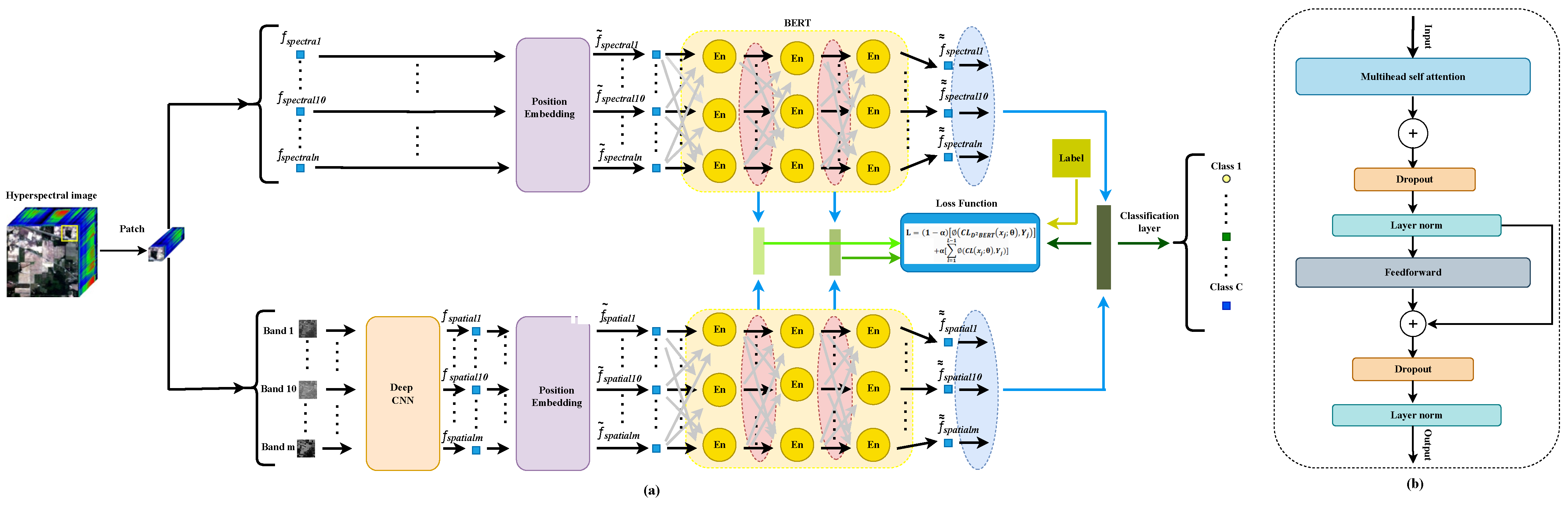
  • To make full use of spatial dependencies among neighboring pixels and spectral dependencies among spectral bands, a dual-dimension (i.e., spatial-spectral) BERT is proposed for HSIC, overcoming the limitations of merely considering the spatial dependency as in HSI-BERT.
  • To exploit long-range spectral dependence among spectral bands for HSIC, a spectral BERT branch is introduced, where a band position embedding is integrated to build a band-order-aware network.
  • To improve the learning efficiency of the proposed BERT model, a multi-supervision strategy is presented for training, which allows features from each layer to be directly supervised through the proposed loss function.
An overview of the main parts of the D2BERT model is discussed in Section 2. The results of our experiments are presented in Section 3, and the conclusions are presented in Section 4.

2. Proposed D2BERT Model

As shown in Figure 1, the D2BERT model has two branches to extract the optimal distinctive features for HSIC. In the upper branch, the spatial BERT is used to explore the spatial dependency for the given HSI, while in the bottom branch, a spectral BERT is introduced to explore the spectral dependency. D2BERT combines these spatial-spectral features from the two branches and this model is learned by multiple supervision of features from each intermediate BERT layer.

2.1. Deep Spatial Feature Learning in Spatial BERT

The upper branch, i.e., the spatial branch, aims to determine long-range relationships among pixels in a selected region. In this branch, a square region (patch) containing a target pixel is first selected for label prediction. This area is initially flattened to form a sequential representation that passes through position embedding and stacked spatial encoders. Features extracted by these encoders are given in input to classification layers for multi-layer supervision. More in detail, each patch is flattened to create a pixel sequence ( f s p e c t r a l 1 , , f s p e c t r a l 10 , , f s p e c t r a l n ). The positional embedding (PE) module is fed by the flattened patch. The PE learns positional embeddings and works independently and identically for each pixel [27]. The PE encodes the positional information. Thus, we have:
f ˜ spectral = f spectral + p ,
where f ˜ spectral is the learned positional embedding and p is the learned positional element.
The BERT module receives these features that are enhanced by the stacked spatial BERT encoders, see Figure 1. A BERT encoder consists of a multi-head self-attention (MHSA), a feedforward network, layer norms, and dropouts. MHSA captures different aspects, by different heads, of the relationships among pixels in the patch [28]. Each attention function can be defined as a mathematical operation that takes a query vector and a set of key-value pairs as inputs and produces an output vector. In this context, vectors represent the query, the keys, the values, and the output. Different heads are related to distinct attentions. All heads operate independently and concurrently. There is a global receptive field for each head in the patch. The scaled dot-product attention is used to calculate all the attention distributions. The final result is calculated by adding all the weighted values. The importance of each value is computed using a compatibility function that compares the query to each key:
Attention ( Q , K , V ) = softmax Q K T d k V ,
where Q , K , V , and d k denote the query, the key, the value, and the dimension of the data in the input. The feedforward process affects all heads by utilizing interconnected layers to enhance and refine the learned characteristics. A ReLU activation separates two linear layers in the feedforward. All encoders share the same feedforward network. Thus, we ensure that the parameters of the feedforward layer are the same in all encoders. During the model training, layer normalization decreases the internal covariate shift. The layer normalization provides several advantages (e.g., the training becomes more efficient allowing for higher learning rates). The extracted features from the spatial BERT branch ( f ˜ ˜ spectral 1 , , f ˜ ˜ spectral 10 , , f ˜ ˜ spectral n ) are then injected into the classification layer.

2.2. Deep Spectral Feature Learning in Spectral BERT

The spectral branch is similar to the spatial branch. The goal of this branch is to determine long-range relationships among spectral bands in a selected region. Initially, in the patch, all HSI bands are separated. Suppose that there are m spectral bands ( B a n d 1 , , B a n d 10 , , B a n d m ). The information of each band is represented by a vector of spatial features. A deep 2-D CNN model is used to extract spatial features for each band. In this study, we used the VGG-like architecture, in which several convolutional layers are ignored to reduce overfitting [29]. The extracted features ( f s p a t i a l 1 , , f s p a t i a l 10 , , f s p a t i a l m ) are then processed by the position embedding stage, in which the position information of the different bands is added ( f ˜ s p a t i a l 1 , , f ˜ s p a t i a l 10 , , f ˜ s p a t i a l m ). Afterwards, the output of the position embedding stage is the input of the BERT module, see Figure 1. This latter module aims to learn long-range dependencies among spectral bands in the spectral domain. As in the spatial domain, the BERT module can check different relationships among its inputs. The final features of the BERT module are injected into the classification layer.

2.3. D2BERT Model Training

Most of deep-learning hyperspectral image classification models, such as HSI-BERT, are trained based on the one-hot label [26]. However, in the proposed D2BERT model, the hidden information coming from the intermediate layers of the BERT modules is also exploited, thus improving the accuracy of the trained model. Accordingly, D2BERT is trained based on the one-hot label and the multi-layer supervision exploiting intermediate features. Moreover, the extracted features from spatial and spectral branches are combined and then given in input to a classification layer to predict the label of the target pixel.
Suppose that the number of training samples is N and C represents the number of classes. If the i-th (target) pixel, x i , belongs to class j then Y i j = 1 , otherwise Y i j = 0 . The BERT modules consist of L layers. The output features of each layer are transferred to an independent classification layer to predict the label. The input features for each classification layer are obtained by the concatenation of the features, obtained from the two BERT modules on the two (spatio-spectral) branches. We calculate the cross-entropy between the output of each classifier and the one-hot label. Therefore, the loss function given x i , L i , is defined as follows:
L i = ( 1 α ) ϕ ( C L D 2 B E R T ( x i ; θ ) , Y i j ) + α l = 1 L 1 ϕ ( C L ( x i ; θ l ) , Y i j )
where ϕ ( · ) indicates the cross-entropy, C L ( · ) is the output of the classifier of the l-th layer, θ l indicates the network parameters of the l-th BERT block, C L D 2 B E R T ( · ) denotes the classification output, θ shows the overall network parameters of the model, and the weight α balances the contribution of the information coming from the intermediate layers with respect to the one from the output layer.

3. Experimental Analysis

Two datasets have been considered for performance assessment. The first dataset is the Pavia University (PU) dataset containing 610 × 340 pixels with 103 spectral bands. Nine classes are represented in this image with 42,776 labeled pixels. The second dataset is the Indian Pines (IP). The Indian Pines dataset contains 200 bands and 16 land-cover types. This dataset has a spatial dimension of 145 × 145 .

3.1. Experimental Setting

D2BERT is implemented using PyTorch and run on a V100 GPU. For training and testing, we randomly selected 50, 100, 150, or 200 labeled pixels, dividing the data into ten sets. The learning rate was set to 3 × 10 4 with 200 training epochs and a dropout rate 0.2. The model uses three encoder layers and two attention heads to balance complexity and efficiency. Unlike the previous approach, which allowed various region shapes, the proposed method uses 32 × 32 patches for spatial feature extraction using CNNs. The selected metrics for comparison are the overall accuracy (OA), the average accuracy (AA), the training/testing times, and the number of parameters.

3.2. Evaluation Metrics
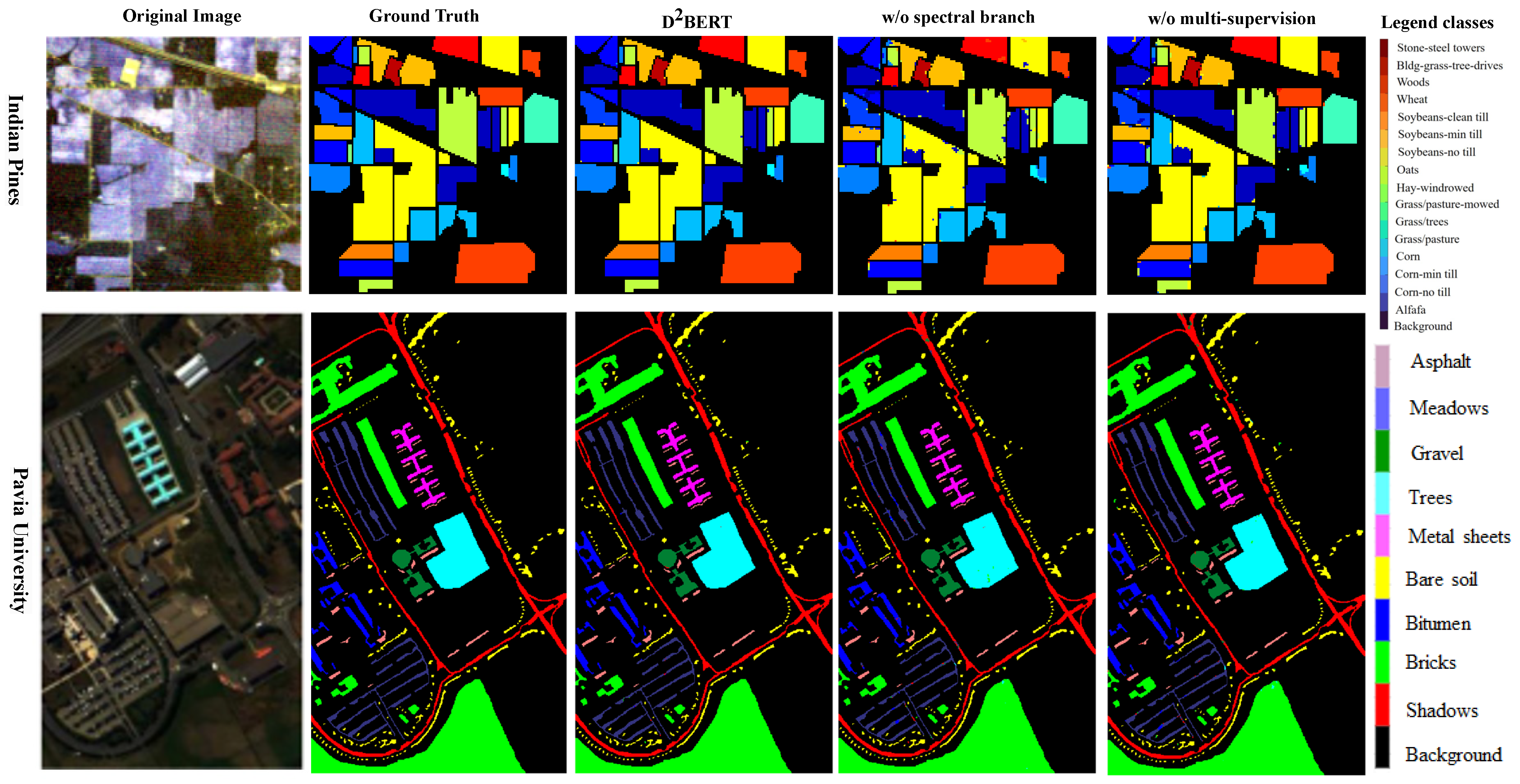
In evaluating the proposed model, two critical metrics are employed: average accuracy (AA) and overall accuracy ( O A ). The overall accuracy, O A , of the model is determined through the equation:
O A = Sum of Correct Predictions ( i X e v a l ) Total Number of Predictions
i X e v a l represents the summation of correct predictions made by the model across all test instances. The denominator, ‘Total Number of Predictions’, corresponds to the entire set of predictions made by the model, encompassing both correct and incorrect predictions.
For assessing the accuracy of individual classes within the dataset, average accuracy ( A A ) is utilized. This is calculated using the following formula:
A A = 1 Classes Count i = 1 n j = 1 X i j C i
where n is the total number of classes, C i denotes the count of instances in the ith class, and X i j represents the jth correct prediction for the ith class.

3.3. Ablation Study

In the proposed method, we claimed that the hidden information among spectral bands can improve the classification performance. In this experiment, this claim is examined. We performed this experiment on both datasets using 200 training samples. The classification accuracies from the D2BERT and D2BERT without the spectral BERT branch are reported in Table 1 and Table 2. It is obvious that D2BERT achieves much better results when the spectral BERT branch is considered. It can be seen that D2BERT achieves the lowest confusion between classes compared to the D2BERT without the spectral BERT branch model. Indeed, we have improved the classification performance, as measured by the OA, by 0.92% and 2.59% for PU and IP, respectively. Moreover, we want to analyze how the use of the intermediate layer information in the loss function impacts the classification accuracy. Hence, we evaluate our method without incorporating intermediate layer information in the loss function. The classification results are reported in Table 1 and Table 2. It is clear that layer information in the loss function plays a crucial role leading to performance reduction when it is neglected. The OA is improved by 0.72% and 1.74% for PU and IP, respectively. The corresponding classification maps for these two ablation experiments are depicted in Figure 2. Overall, D2BERT has shown superior performance compared to the ablated models on both datasets in terms of fewer misclassifications, especially for more challenging classes. This demonstrates the effectiveness of capturing spatial and spectral dependencies simultaneously using dual BERT branches, as well as utilizing intermediate layers during optimization. Although the performance gaps differ between datasets, they consistently suggest the significance of both proposed contributions toward achieving state-of-the-art hyperspectral classification.

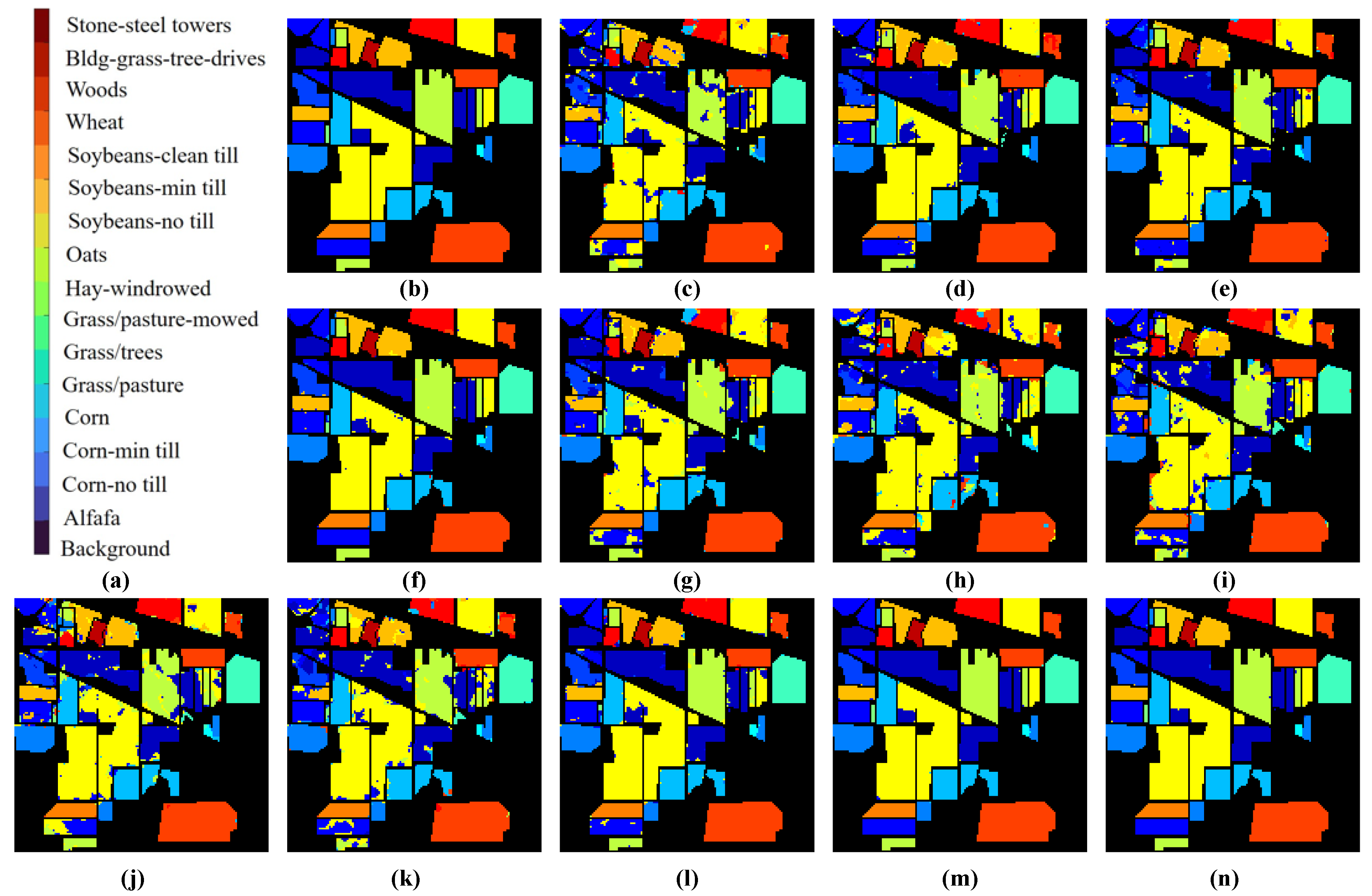
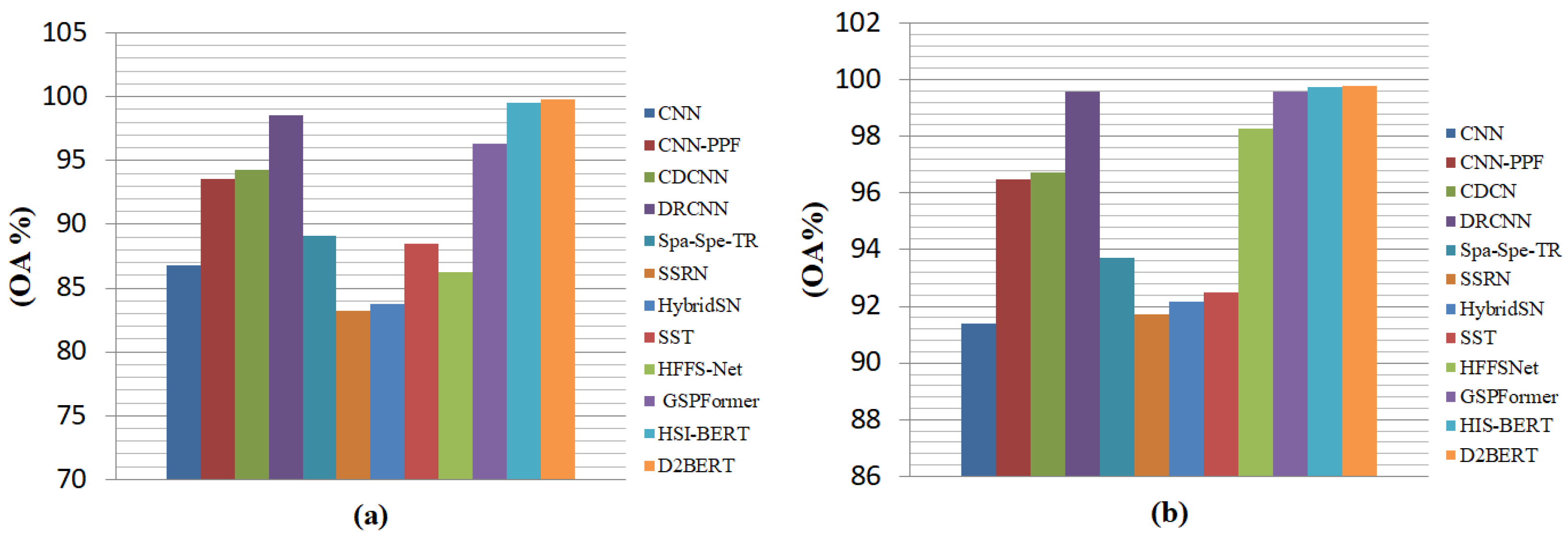
3.4. Comparison with Benchmark

This section is devoted to the comparison of the proposed D2BERT approach with state-of-the-art CNN-based, transformer-based, and BERT-based methods, i.e., CNN [22], CNN-PPF [30], CDCNN [31], DRCNN [31], Spa-Spe-TR [32], SSRN [33], HybridSN [34], SST [32], HFFSNet [35], GSPFormer [36], and HSI-BERT [26]. The first analysis is based on the comparison of the proposed approach varying the number of samples for training (i.e., 50, 100, 150, and 200) and using the rest of the dataset for testing. Some exemplary methods belonging to our benchmark have been selected for the sake of clarity, including the previously developed HSI BERT and some CNN-based methods. The classification performance varying the number of samples is depicted in Table 3. The better performance of the proposed method is clear, with OA always greater than one of the other techniques, whatever the number of training samples.
The proposed model consistently outperforms all five contemporary CNN-based methods, including HSI-BERT. Thus, D2BERT exhibits a distinct advantage over CNN-based approaches when dealing with limited training samples.
The second analysis relies upon the calculation of the OA and AA indexes for all the compared approaches, training them with 200 samples. The results are reported in Table 4, the classified maps achieved from the comparing methods are presented in Figure 3 and the OA graphs are presented in Figure 4. Among the compared methods on the Pavia University dataset, D2BERT achieves the highest OA and AA indexes, i.e., 99.79% and 99.68%, respectively. The gap in performance is clear with respect to CNN, Spa-Spe-TR, SSRN, HybridSN, and SST, with improvements in the range from 6.07% to 8.38%. D2BERT achieves the same remarkable level of accuracy as DRCNN, HSI-BERT, HFFSNet, and GSPFormer. These results point out the superiority of D2BERT in accurately classifying the Pavia University data. Focusing on the Indian Pine dataset, D2BERT achieves very high values of the OA and AA indexes, i.e., 99.76% and 99.68%, respectively, obtaining the top scores among the compared approaches. The comparison of the classification maps also shows the superiority of D2BERT. These experiments demonstrate that D2BERT achieves state-of-the-art classification performance on two benchmark datasets compared to recent CNN, transformer, and BERT-based methods.
Nonetheless, D2BERT demonstrates exceptional classification performance, indicating its effectiveness in accurately classifying the Indian Pine dataset. D2BERT offers advantages in hyperspectral image classification by capturing global and local dependencies, utilizing a neural language-based model, employing BERT modules, and incorporating spectral and spatial features. It explores relations between pixels and spectral bands, reduces complexity, and uses intermediate information for enhanced performance.
D2BERT is a high-performing model for HSIC, exploiting global and local dependencies, BERT modules, and spectral/spatial features. It efficiently explores relations among pixels and spectral bands, reducing complexity and using intermediate layer information to improve performance. Despite a longer training time than HSI-BERT, D2BERT excels in understanding data dependencies and semantic relationships, achieving a higher performance. Results about the computational burden of the compared approaches are reported in Table 5. D2BERT stands out as the most efficient model, on par with HSI-BERT, due to its relatively shallow architecture and concurrent execution of individual heads in the MHSA. Moreover, D2BERT’s parameter count is comparable to other methods, making it a competitive choice in hyperspectral image classification tasks. However, some limitations remain. First, D2BERT incurs higher memory and computational costs than traditional CNN models due to the introduction of transformers. Second, the model may not fully capture fine-grained spatial patterns at small scales due to the use of relatively large patches. Nonetheless, D2BERT also holds promising potential. Its dual-branch architecture is easily parallelizable, aiding runtime efficiency. Transformers allow modeling long-range dependencies beyond the limitations of patch-based CNN receptive fields. The main idea for future work is to investigate how lightweight transformer variants could improve efficiency while maintaining accuracy

4. Conclusions

In this paper, an image classification model based on BERT, the so-called D2BERT, has been proposed. It relies upon a dual-dimensional spatial-spectral classification in which global and local relations and dependencies among neighboring pixels are investigated, considering both the spatial and spectral domains. D2BERT exploits two BERT modules to explore spatial and spectral dependencies among pixels belonging to a selected region. The intermediate information coming from different layers of the BERT modules has been considered in the loss function, improving the performance of the model. Experimental results demonstrated the high accuracy of the proposed model outperforming state-of-the-art CNN, transformer, and BERT methods. Experimental results on two benchmark datasets demonstrated the effectiveness of D2BERT. On the PU dataset with 200 training samples, D2BERT achieved an OA of 99.79%, outperforming the second-best method (HSI-BERT) by over 0.04%. On the more challenging IP dataset, D2BERT attained an overall accuracy of 99.76%, outperforming the second-best method (HSI-BERT) by over 0.2%. When limited training data (50 samples) was used, D2BERT improved overall accuracy over HSI-BERT by 1.18% on PU and 1.94% on IP, validating its advantages in low data regimes. Ablation studies showed removing either the spectral branch or multi-supervision lowered accuracy, demonstrating the importance of both contributions.

Author Contributions

Conceptualization, M.A. and L.C.; methodology, M.A. and R.S.M.; software, M.A.; validation, L.C. and X.Z.; formal analysis, L.C.; investigation, X.Z.; resources, X.Z.; data curation, R.S.M.; writing—original draft preparation, M.A. and L.C.; writing—review and editing, Gemine Vivone and R.C.; visualization, M.A. and L.C.; supervision, L.C.; project administration, X.Z.; funding acquisition, X.Z. and L.C. All authors have read and agreed to the published version of the manuscript.

Funding

This work is supported in part by the National Natural Science Foundation of China under Grant 62301093, Grant 61971072, Grant U2133211, and under Grant 62001063, in part by the Postdoctoral Fellowship Program of CPSF under Grant GZC20233336, in part by the China Postdoctoral Science Foundation under Grant 2023M730425, and in part by the Fundamental Research Funds for the Central Universities under Project No. 2023CDJXY-037.

Data Availability Statement

The datasets utilized in this research are publicly available and can be accessed via the URL https://www.ehu.eus/ccwintco/index.php/Hyperspectral_Remote_Sensing_Scenes (accessed on 15 September 2023). The specific details regarding the datasets, including any necessary information on how to access or cite them, can be found at the provided URL(s). All data used in this study can be freely obtained from the aforementioned source.

Acknowledgments

The authors thank the Editors who handled this manuscript and the anonymous reviewers for their outstanding comments and suggestions

Conflicts of Interest

The authors declare no conflict of interest.

References

  1. Yu, C.; Huang, J.; Song, M.; Wang, Y.; Chang, C.I. Edge-inferring graph neural network with dynamic task-guided self-diagnosis for few-shot hyperspectral image classification. IEEE Trans. Geosci. Remote Sens. 2022, 60, 1–13. [Google Scholar] [CrossRef]
  2. Wang, Y.; Chen, X.; Zhao, E.; Song, M. Self-supervised Spectral-level Contrastive Learning for Hyperspectral Target Detection. IEEE Trans. Geosci. Remote Sens. 2023, 61, 1–15. [Google Scholar] [CrossRef]
  3. Guha, A. Mineral exploration using hyperspectral data. In Hyperspectral Remote Sensing; Elsevier: Amsterdam, The Netherlands, 2020; pp. 293–318. [Google Scholar]
  4. Aspinall, R.J.; Marcus, W.A.; Boardman, J.W. Considerations in collecting, processing, and analysing high spatial resolution hyperspectral data for environmental investigations. J. Geogr. Syst. 2002, 4, 15–29. [Google Scholar] [CrossRef]
  5. Caballero, D.; Calvini, R.; Amigo, J.M. Hyperspectral imaging in crop fields: Precision agriculture. In Data Handling in Science and Technology; Elsevier: Amsterdam, The Netherlands, 2019; Volume 32, pp. 453–473. [Google Scholar]
  6. Benediktsson, J.A.; Palmason, J.A.; Sveinsson, J.R. Classification of hyperspectral data from urban areas based on extended morphological profiles. IEEE Trans. Geosci. Remote Sens. 2005, 43, 480–491. [Google Scholar] [CrossRef]
  7. Zhao, F.; Zhang, J.; Meng, Z.; Liu, H. Densely connected pyramidal dilated convolutional network for hyperspectral image classification. Remote Sens. 2021, 13, 3396. [Google Scholar] [CrossRef]
  8. Hong, D.; Han, Z.; Yao, J.; Gao, L.; Zhang, B.; Plaza, A.; Chanussot, J. SpectralFormer: Rethinking hyperspectral image classification with transformers. IEEE Trans. Geosci. Remote Sens. 2021, 60, 1–15. [Google Scholar] [CrossRef]
  9. Scheibenreif, L.; Mommert, M.; Borth, D. Masked Vision Transformers for Hyperspectral Image Classification. In Proceedings of the IEEE/CVF Conference on Computer Vision and Pattern Recognition, Vancouver, BC, Canada, 17–24 June 2023; pp. 2165–2175. [Google Scholar]
  10. Fang, L.; Li, S.; Duan, W.; Ren, J.; Benediktsson, J.A. Classification of hyperspectral images by exploiting spectral-spatial information of superpixel via multiple kernels. IEEE Trans. Geosci. Remote Sens. 2015, 53, 6663–6674. [Google Scholar] [CrossRef]
  11. Majdar, R.S.; Ghassemian, H. Improved Locality Preserving Projection for Hyperspectral Image Classification in Probabilistic Framework. Int. J. Pattern Recognit. Artif. Intell. 2021, 35, 2150042. [Google Scholar] [CrossRef]
  12. Marconcini, M.; Camps-Valls, G.; Bruzzone, L. A composite semisupervised SVM for classification of hyperspectral images. IEEE Geosci. Remote Sens. Lett. 2009, 6, 234–238. [Google Scholar] [CrossRef]
  13. Ye, Q.; Zhao, H.; Li, Z.; Yang, X.; Gao, S.; Yin, T.; Ye, N. L1-Norm distance minimization-based fast robust twin support vector k-plane clustering. IEEE Trans. Neural Netw. Learn. Syst. 2017, 29, 4494–4503. [Google Scholar] [CrossRef]
  14. Pal, M. Multinomial logistic regression-based feature selection for hyperspectral data. Int. J. Appl. Earth Obs. Geoinf. 2012, 14, 214–220. [Google Scholar] [CrossRef]
  15. Yang, J.M.; Yu, P.T.; Kuo, B.C. A nonparametric feature extraction and its application to nearest neighbor classification for hyperspectral image data. IEEE Trans. Geosci. Remote Sens. 2009, 48, 1279–1293. [Google Scholar] [CrossRef]
  16. Samaniego, L.; Bárdossy, A.; Schulz, K. Supervised classification of remotely sensed imagery using a modified k-NN technique. IEEE Trans. Geosci. Remote Sens. 2008, 46, 2112–2125. [Google Scholar] [CrossRef]
  17. Li, W.; Du, Q.; Zhang, F.; Hu, W. Collaborative-representation-based nearest neighbor classifier for hyperspectral imagery. IEEE Geosci. Remote Sens. Lett. 2014, 12, 389–393. [Google Scholar] [CrossRef]
  18. Sun, L.; Wu, Z.; Liu, J.; Xiao, L.; Wei, Z. Supervised spectral–spatial hyperspectral image classification with weighted Markov random fields. IEEE Trans. Geosci. Remote Sens. 2014, 53, 1490–1503. [Google Scholar] [CrossRef]
  19. Tarabalka, Y.; Fauvel, M.; Chanussot, J.; Benediktsson, J.A. SVM-and MRF-based method for accurate classification of hyperspectral images. IEEE Geosci. Remote Sens. Lett. 2010, 7, 736–740. [Google Scholar] [CrossRef]
  20. Rodarmel, C.; Shan, J. Principal component analysis for hyperspectral image classification. Surv. Land Inf. Sci. 2002, 62, 115–122. [Google Scholar]
  21. Cheng, G.; Li, Z.; Han, J.; Yao, X.; Guo, L. Exploring hierarchical convolutional features for hyperspectral image classification. IEEE Trans. Geosci. Remote Sens. 2018, 56, 6712–6722. [Google Scholar] [CrossRef]
  22. Lee, H.; Kwon, H. Contextual deep CNN based hyperspectral classification. In Proceedings of the 2016 IEEE International Geoscience and Remote Sensing Symposium (IGARSS), Beijing, China, 10–15 July 2016; IEEE: Piscataway, NJ, USA, 2016; pp. 3322–3325. [Google Scholar]
  23. Xu, X.; Li, W.; Ran, Q.; Du, Q.; Gao, L.; Zhang, B. Multisource remote sensing data classification based on convolutional neural network. IEEE Trans. Geosci. Remote Sens. 2017, 56, 937–949. [Google Scholar] [CrossRef]
  24. Cao, X.; Yao, J.; Xu, Z.; Meng, D. Hyperspectral image classification with convolutional neural network and active learning. IEEE Trans. Geosci. Remote Sens. 2020, 58, 4604–4616. [Google Scholar] [CrossRef]
  25. Mou, L.; Ghamisi, P.; Zhu, X.X. Deep recurrent neural networks for hyperspectral image classification. IEEE Trans. Geosci. Remote Sens. 2017, 55, 3639–3655. [Google Scholar] [CrossRef]
  26. He, J.; Zhao, L.; Yang, H.; Zhang, M.; Li, W. HSI-BERT: Hyperspectral image classification using the bidirectional encoder representation from transformers. IEEE Trans. Geosci. Remote Sens. 2019, 58, 165–178. [Google Scholar] [CrossRef]
  27. Devlin, J.; Chang, M.W.; Lee, K.; Toutanova, K. Bert: Pre-training of deep bidirectional transformers for language understanding. arXiv 2018, arXiv:1810.04805. [Google Scholar]
  28. Dehghani, M.; Gouws, S.; Vinyals, O.; Uszkoreit, J.; Kaiser, Ł. Universal transformers. arXiv 2018, arXiv:1807.03819. [Google Scholar]
  29. Windrim, L.; Melkumyan, A.; Murphy, R.J.; Chlingaryan, A.; Ramakrishnan, R. Pretraining for hyperspectral convolutional neural network classification. IEEE Trans. Geosci. Remote Sens. 2018, 56, 2798–2810. [Google Scholar] [CrossRef]
  30. Li, W.; Wu, G.; Zhang, F.; Du, Q. Hyperspectral image classification using deep pixel-pair features. IEEE Trans. Geosci. Remote Sens. 2016, 55, 844–853. [Google Scholar] [CrossRef]
  31. Lee, H.; Kwon, H. Going deeper with contextual CNN for hyperspectral image classification. IEEE Trans. Image Process. 2017, 26, 4843–4855. [Google Scholar] [CrossRef] [PubMed]
  32. He, X.; Chen, Y.; Li, Q. Two-Branch Pure Transformer for Hyperspectral Image Classification. IEEE Geosci. Remote Sens. Lett. 2022, 19, 1–5. [Google Scholar] [CrossRef]
  33. Zhong, Z.; Li, J.; Luo, Z.; Chapman, M. Spectral–spatial residual network for hyperspectral image classification: A 3-D deep learning framework. IEEE Trans. Geosci. Remote Sens. 2017, 56, 847–858. [Google Scholar] [CrossRef]
  34. Roy, S.K.; Krishna, G.; Dubey, S.R.; Chaudhuri, B.B. HybridSN: Exploring 3-D–2-D CNN feature hierarchy for hyperspectral image classification. IEEE Geosci. Remote Sens. Lett. 2019, 17, 277–281. [Google Scholar] [CrossRef]
  35. Feng, Z.; Liu, X.; Yang, S.; Zhang, K.; Jiao, L. Hierarchical Feature Fusion and Selection for Hyperspectral Image Classification. IEEE Geosci. Remote Sens. Lett. 2023, 20, 1–5. [Google Scholar] [CrossRef]
  36. Chen, D.; Zhang, J.; Guo, Q.; Wang, L. Hyperspectral Image Classification based on Global Spectral Projection and Space Aggregation. IEEE Geosci. Remote Sens. Lett. 2023, 20, 1–5. [Google Scholar] [CrossRef]
Figure 1. (a) The proposed D2BERT model. (b) Encoder (En) layer.
Remotesensing 16 00539 g001
Figure 2. Classification maps achieved by D2BERT in three different configurations and the ground-truth for IP and PU.
Remotesensing 16 00539 g002
Figure 3. Classification maps of IP achieved by different methods (a) classes, (b) ground truth, (c) CNN, (d) CNN-PPF, (e) CDCNN, (f) DRCNN, (g) Spa-Spe-TR, (h) SSRN, (i) HybridSN, (j) SST, (k) HFFSNet, (l) GSPFormer, (m) HSI-BERT, (n) D2BERT.
Remotesensing 16 00539 g003
Figure 4. Classification accuracy varying the number of training samples: (a) PU, (b) IP.
Remotesensing 16 00539 g004
Table 1. Classification results of different D2BERT configurations for the Pavia University (PU) dataset.
ClassD2BERT w/o
Spectral Branch
D2BERT w/o
Multi-Supervision
D2BERT
195.83100100
295.8298.2199.54
396.2196.0799.60
497.1099.00100
597.7395.5298.32
698.9499.69100
786.9686.96100
81.00100100
91.0082.35100
OA (%)98.88 ± 0.1099.04 ± 0.1199.79 ± 0.06
AA (%)98.36 ± 0.1898.42 ± 0.1499.68 ± 0.09
Table 2. Classification results of different D2BERT configurations for the Indian Pines (IP) dataset.
ClassD2BERT w/o
Spectral Branch
D2BERT w/o
Multi-Supervision
D2BERT
198.8998.7599.93
299.7899.8599.98
396.2697.9898.85
497.4498.0199.41
5100100100
699.4499.98100
798.7196.8199.91
895.7495.6699.02
998.8698.62100
1094.4097.8599.83
1197.3097.8799.86
1294.4898.09100
1399.4798.90100
1499.56100100
1599.7096.60100
161.0092.6898.25
OA (%)99.04 ± 0.1198.05 ± 0.2799.76 ± 0.03
AA (%)97.09 ± 1.2696.22 ± 0.7099.71 ± 0.05
Table 3. Classification results (OA%) of IP with different models using different numbers of training samples. Best results are in boldface
Dataset
# Samples
PUIP
5010015020050100150200
CNN86.3988.590.8991.4180.4384.3285.3086.81
CNN-PPF88.1493.3595.596.4888.3491.7293.1493.90
CDCNN92.1993.5595.596.7384.4388.2792.2594.24
DRCNN96.9198.6799.2199.5688.7494.9497.4998.54
HSI-BERT97.4398.7899.3899.7591.3196.8698.0399.56
D2BERT98.5899.3599.7399.7993.0998.2699.1499.76
Table 4. Classification accuracy (%) of the compared approaches. The best results are in boldface.
Dataset
Methods
Pavia UniversityIndian Pines
OA%AA%OA%AA%
CNN91.4181.0386.8163.30
CNN-PPF96.4897.0393.6096.38
CDCNN96.7395.7794.2495.75
DRCNN99.5698.2298.5499.29
Spa-Spe-TR93.7291.0089.1375.23
SSRN91.7287.5683.2168.88
HybridSN92.1885.1683.7763.18
SST92.5085.1688.5166.64
HFFSNet98.2797.2086.2183.53
GSPFormer99.5699.2596.2992.60
HSI-BERT99.7599.8699.5699.72
D2BERT99.7999.6899.7699.71
Table 5. Training times, testing times, and a number of parameters for the compared approaches. H, S, and M stand for hours, seconds, and millions, respectively. The best results are in boldface.
Training Time (Hours)
Pavia UniversityIndian Pines# Parameters
MethodsTrain (H)Test (S)Train (H)Test (S)in (M)
CNN0.310.370.390.210.13
CNN-PPF1.0016.926.004.760.05
CDCNN0.1312.350.1411.211.12
DRCNN0.431050.74390.05
Spa-Spe-TR0.1649.20.1419.8027.65
SSRN1.280.342.210.060.23
HybridSN0.0220.40.033.614.85
SST16.690.7821.430.1929
HFFSNet0.022.510.023.4532.74
GSPFormer0.47530.18120.68
HSI-BERT0.079.280.123.521.21
D2BERT0.1916.410.269.112.45
Disclaimer/Publisher’s Note: The statements, opinions and data contained in all publications are solely those of the individual author(s) and contributor(s) and not of MDPI and/or the editor(s). MDPI and/or the editor(s) disclaim responsibility for any injury to people or property resulting from any ideas, methods, instructions or products referred to in the content.

