Time Lag and Cumulative Effects of Extreme Climate on Coastal Vegetation in China

Abstract

Rapid global changes are altering regional hydrothermal conditions, especially in ecologically vulnerable areas such as coastal regions, subsequently influencing the dynamics of vegetation growth. However, there is limited research investigating the response of vegetation in these regions to extreme climates and the associated time lag-accumulation relationships. This study utilized a combined approach of gradual and abrupt analysis to examine the spatiotemporal patterns of vegetation dynamics in the coastal provinces of China from 2000 to 2019. Additionally, we evaluated the time lag-accumulation response of vegetation to extreme climate events. The results showed that (1) extreme high temperatures and extreme precipitation had increased over the past two decades, with greater warming observed in high latitudes and concentrated precipitation increases in water-rich southern regions; (2) both gradual and abrupt analyses indicate significant vegetation improvement in coastal provinces; (3) significant lag-accumulation relationships were observed between vegetation and extreme climate in the coastal regions of China, and the time-accumulation effects were stronger than the time lag effects. The accumulation time of extreme temperatures was typically less than one month, and the accumulation time of extreme precipitation was 2–3 months. These findings are important for predicting the growth trend of coastal vegetation, understanding environmental changes, and anticipating ecosystem evolution.

1. Introduction

As a critical link between solar and biotic energy, vegetation significantly contributes to ecosystems by enhancing soil conditions, maintaining ecosystem stability, regulating carbon balance, supporting hydrological cycles, and mitigating greenhouse gas emissions [1,2,3]. The changes in vegetation structure and function are driven by a combination of climate and environmental variations, as well as anthropogenic activities such as land use changes [4]. Climate change primarily affects terrestrial ecosystems, mainly by altering critical processes such as plant respiration, photosynthesis, growing seasons, and soil formation, which can have long-term repercussions on the spatial distribution patterns of vegetation [5]. Current reports and forecasts indicate a consistent trend of global warming, underscoring the increased likelihood of more frequent and intense extreme climate events [6]. Different countries and regions around the world have experienced more frequent and intense extreme weather events such as droughts and heatwaves [7,8]. The responses of vegetation to climate are often intricate, and long-term climate changes result in gradual alterations in vegetation distribution and dynamics, while extreme climatic events exert significant rapid impacts on vegetation [9]. Hence, unveiling substantial alterations in global climate conditions, comprehending the influence of extreme climatic events on vegetation dynamics, and assessing the mechanisms behind these interactions are all crucial for understanding the uncertainties associated with vegetation growth and ecosystem carbon sequestration in response to climate change.

The vegetation status is a crucial indicator reflecting the evolution of the natural ecological environment. Conducting vegetation change monitoring is a fundamental requirement for evaluating the quality and suitability of the ecological environment [10]. Previous research has highlighted that vegetation indices based on “greenness” observations, such as the normalized difference vegetation index (NDVI), can only detect the “potential photosynthesis” of plants [11]. They may fail to capture variations in photosynthesis for certain vegetation types such as evergreen forests, as “greenness” and photosynthesis are occasionally decoupled [12]. Inaccurate estimation of vegetation growth based on “greenness” can introduce substantial uncertainty in estimating vegetation productivity and carbon sequestration [13,14]. The emergence of satellite-based solar-induced chlorophyll fluorescence (SIF) offers an unprecedented opportunity for more accurate tracking of actual vegetation growth [15,16]. Unlike canopy reflectance products, SIF is a by-product of vegetation photosynthesis and is tightly coupled with the photosynthetic process, allowing it to reflect changes in vegetation physiology at the onset of change, making it a more sensitive method of detecting vegetation photosynthetic physiology than traditional vegetation indices [17]. It can better capture the growth status of evergreen vegetation and arid ecosystems, especially in the early stages of vegetation stress [18,19].

Characterizing temporal changes in vegetation primarily involves two types: gradual and abrupt [20]. Gradual changes can be determined using linear trends or Sen’s trends, with the slope value indicating the direction and rate of vegetation change over time [21]. Gradual analysis assumes that the vegetation change trend remains constant throughout the period. However, growth processes may not always rise or fall steadily in the long-term trend of vegetation change; instead, they are likely to undergo various, potentially opposite, phase trends due to the impact of drought, high temperatures, and afforestation [22,23]. This can lead to certain uncertainties in gradual analysis when assessing the changing characteristics of time-series vegetation indices, potentially obscuring vital abrupt change information [24]. Therefore, it is especially crucial to effectively extract and identify breakpoint types and trends in vegetation growth stages [25]. The breaks for additive season and trend (BFAST) method is widely applied for detecting trend changes in long-time series [26]. It can segment the overall trend into multiple segments. As a result, in monitoring vegetation growth dynamics, it is necessary to combine gradual and abrupt analysis to avoid overlooking the true vegetation trends and fluctuations due to inadequate focus on either gradual or abrupt characteristics.

The growth status of vegetation is closely related to climate change patterns, and plants typically exhibit non-linear responses to climate change [27,28]. Climate change only induces inevitable vegetation changes when it accumulates beyond the environmental carrying capacity or the vegetation’s tolerance. This suggests that climate change processes involve a time lag in vegetation dynamics in response to climate [29]. Damage to growth only occurs when climate passes a critical threshold. Compared to average climate change, extreme climatic events possess characteristics of suddenness, unpredictability, and destructiveness [30]. Extreme climates typically have the potential to impact terrestrial ecosystems in various ways, such as reducing primary productivity and altering carbon budgets. They can also force species to adapt to changing environments and, in some cases, increase the risk of local species decline or even extinction [31]. The impacts of extreme climates on the ecological environment are more direct and severe [32]. Therefore, understanding the relationship between extreme climates and vegetation is crucial for assessing the adaptability and vulnerability of vegetation to extreme climates, and promoting adaptation and mitigation strategies for extreme climates. Many researchers have assessed the impact of extreme climate events (heatwaves, droughts, extreme precipitation) on vegetation from various perspectives [33,34]. However, in most previous studies, the focus has been predominantly on examining the correlation between vegetation indices and extreme climate indices, using the magnitude of the correlation coefficient to determine the extent of the impact of extreme climate on vegetation [35,36]. Nevertheless, there has been relatively little attention given to the analysis of the lag-accumulation effects of extreme climate events on vegetation. Lag effects or temporal cumulative effects may exist in the interaction between vegetation and climate change [37]. When climate changes exceed the vegetation’s tolerance threshold, vegetation responds through feedback mechanisms. In other words, the dynamic response of vegetation to climate variability may not be immediate [38]. Lag effects refer to the impact of climate conditions changing at a specific time on the current vegetation, implying that the influence of climate changes a few months earlier is more significant for current vegetation growth [39]. Time accumulation effects indicate that vegetation growth is notably influenced by the cumulative climate conditions from the past few months, including the current month [40]. The response of vegetation to climate change exhibits characteristics across multiple time scales, involving not only monthly lags but also potentially seasonal and annual delays [41,42]. Previous research at the global scale has revealed that the time lag effects on various vegetation forms and climate factors differ [43]. Specifically, the time lag-accumulation patterns in vegetation responses to climate within the same ecosystem may vary, while the time lag-accumulation patterns in vegetation responses to climate across different ecosystems may be similar. For instance, the time lag for plant communities in response to monthly maximum temperatures in mid-high latitude regions (such as the Qinghai-Tibet Plateau and the Brazilian Plateau) is relatively long (>12 months) [44].

To date, numerous studies have identified coexisting time lag or cumulative effects of climate factors and extreme climates on vegetation [45,46,47,48,49]. However, research on the time lag-accumulation effects of extreme climates on SIF remains limited, especially in the climatically complex and ecologically diverse coastal regions of China. This limitation restricts our ability to assess and attribute extreme surface phenomena, introducing uncertainty when predicting vegetation growth and ecosystem carbon sequestration responses to climate change [50]. Based on this, this study examines the spatiotemporal characteristics of vegetation activity and its response to extreme climates in the coastal provinces of China from 2000 to 2019. The innovation here lies in bridging the gap in our understanding of how extreme climate events impact sensitive coastal vegetation areas over time. Specifically, this study seeks to (1) explore the spatiotemporal evolution of vegetation activities in the coastal provinces of China using Global OCO-2 SIF dataset (GOSIF) data, in conjunction with gradual and abrupt change analyses; (2) clarify the interannual variability of trends and spatial patterns of extreme climate time series changes; and (3) estimate the relationship between extreme climate and vegetation at the pixel level, and investigate their lag-accumulation effects. This study aims to address knowledge gaps regarding the temporal lag effects of extreme climates on vulnerable coastal vegetation. The outcomes will establish a foundation for forecasting trends in coastal vegetation growth, understanding environmental shifts, and anticipating ecosystem evolution.

2. Materials and Methods

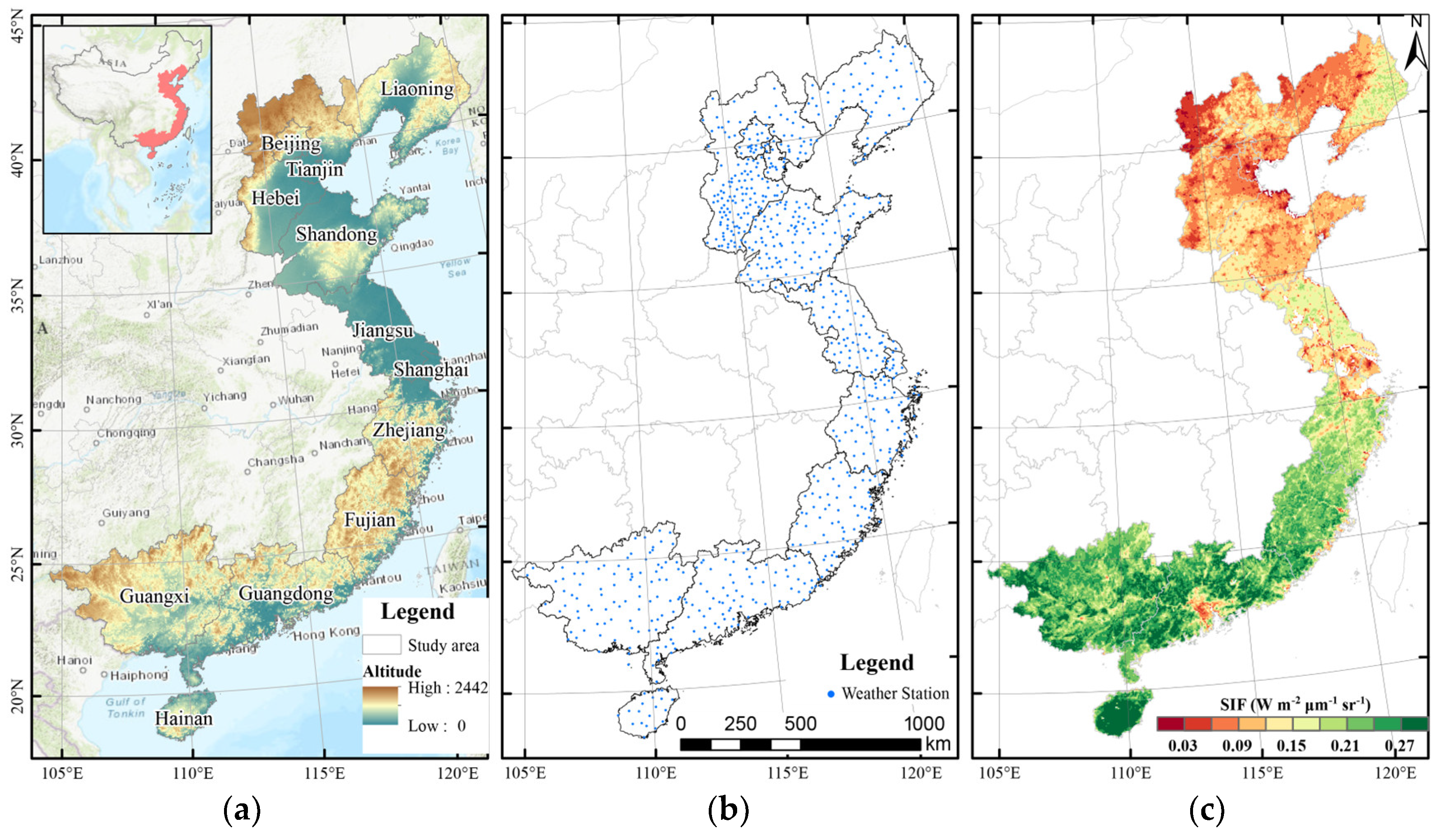
2.1. Study Area

The coastal province of mainland China is situated between approximately 104°26′ and 125°78′E longitude and between 18°16′ and 43°48′N latitude. This region experiences an annual precipitation of around 888.44 mm and an average temperature of approximately 16.50 °C (source: http://data.cma.cn, accessed on 1 January 2024). The study area is delineated based on provincial administrative boundaries, with the inclusion of 14 regions along with their respective maritime zones and islands, including Liaoning, Hebei, Tianjin, Shandong, Jiangsu, Shanghai, Zhejiang, Fujian, Taiwan, Guangdong, Hong Kong Special Administrative Region, Macau Special Administrative Region, Guangxi Zhuang Autonomous Region, and Hainan Province. Taiwan is excluded from this study due to data availability limitations. Although Beijing is situated inland, it is relatively close to the coast, surrounded by two coastal provinces and municipalities, Hebei and Tianjin. To ensure the spatial integrity of the study area and to facilitate a comprehensive and detailed understanding of the coastal regions of mainland China, Beijing has been included in the research scope [51], as shown in Figure 1a.

This study area presents diverse and intricate natural conditions that transition from land to sea, with significantly varying climate types and characteristics from north to south [52]. It is markedly influenced by monsoon climates. The northern part falls within the temperate and warm-temperate zones, while the southern part is classified under subtropical and tropical zones. Winters in most regions are characterized by cold and arid conditions, while summers enjoy ample sunshine and abundant rainfall [53]. The natural vegetation types in the study area region mainly consist of temperate deciduous broadleaf forests, temperate deciduous shrublands, subtropical and tropical evergreen needleleaf forests, subtropical evergreen broadleaf forests, and tropical evergreen broadleaf rainforests [54]. In recent years, due to the accelerating pace of global climate change and rapid socioeconomic development in coastal areas, significant changes have occurred in regional vegetation.

2.2. Data Introduction

Meteorological stations in the coastal provinces of China, illustrated in Figure 1b, cover a geographic expanse of 25 latitudinal and 21 longitudinal degrees. Long-term data from 751 stations (2000–2019) sourced from the National Meteorological Science Data Center (http://data.cma.cn, accessed on 1 January 2024) underwent rigorous quality control, involving data cleansing, outlier detection, and gap-filling methods. These stations furnish vital parameters such as average temperature (TEM), maximum temperature (TEMmax), minimum temperature (TEMmin), and daily precipitation (PRE). Spatial interpolation methods were employed for obtaining raster data. The densely and uniformly distributed stations ensure high representativeness for analyzing extreme climatic conditions in the study area.

SIF, a measure of light emitted by plant chlorophyll molecules, is highly correlated with the actual photosynthetic activity of vegetation [55]. To capture vegetation responses to extreme climate events in this study, we utilized the GOSIF dataset spanning from 2000 to 2019 (http://globalecology.unh.edu/, accessed on 1 January 2024). This dataset was developed using a machine learning algorithm, combining surface reflectance from MODIS and solar-induced fluorescence (SIF) data from the Orbiting Carbon Observatory-2 (OCO-2), along with meteorological reanalysis data [56]. The GOSIF dataset used in this study is characterized by a spatial resolution of 0.05° and an 8-day temporal resolution under clear-sky conditions, covering the period from 2000 to 2019. This dataset was selected to mitigate the limitations of discontinuity and coarse resolution present in OCO-2 SIF products. GOSIF data have been widely applied in previous studies related to productivity assessment, carbon cycling, and drought monitoring [57,58]. We extracted monthly mean GOSIF data to match the monthly scale of extreme climate indices.

2.3. Methods

2.3.1. Extraction of Extreme Climate Indices

Considering the time lag and cumulative effects of climate indices on vegetation, this study selected twenty monthly climate indices from the extreme climate indices defined by the Expert Team on Climate Change Detection and Indices (ETCCDI), which encompass eight precipitation factors and twelve temperature factors (

Table 1. Description of the 20 climatic indices.

ID	Name	Definition	Unit
TEM	TEM	Average temperature: Monthly average value of daily average temperature	°C
TEMmax	Tmax	Monthly average value of daily maximum temperature	°C
TEMmin	Tmin	Monthly average value of daily minimum temperature	°C
DTR	Temperature duration	Monthly mean value of the difference between daily maximum and minimum temperature	°C
TN10p	Cold nights	Number of days when TN < 10th percentile	Days
TX10p	Cold days	Number of days when TX < 10th percentile	Days
TN90p	Warm nights	Number of days when TN < 90th percentile	Days
TX90p	Warm days	Number of days when TX < 90th percentile	Days
TNn	Min Tmin	Monthly minimum value of daily minimum temperature °C	°C
TNx	Max Tmin	Monthly maximum value of daily minimum temperature °C	°C
TXn	Min Tmax	Monthly minimum value of daily maximum temperature °C	°C
TXx	Max Tmax	Monthly maximum value of daily maximum temperature °C	°C
PREF	PRE	Precipitation: Monthly total amount of precipitation	mm
LR	Light rainfall	Monthly total amount of daily precipitation in the range of 0–10 mm	mm
MR	Moderate rainfall	Monthly total amount of daily precipitation in the range of 10–25 mm	mm
HR	Heavy rainfall	Monthly total amount of daily precipitation in the range of 25–50 mm	mm
TR	Torrential rainfall	Monthly total amount of daily precipitation over 50 mm	mm
RX1day	Max 1-day precipitation amount	Monthly maximum 1-day precipitation	mm
RX5day	Max 5-day precipitation amount	Monthly maximum consecutive 5-day precipitation	mm
SDII	Daily precipitation intensity	The ratio of the total amount of precipitation ≥ 1 mm to the number of precipitation days	mm/day

). These twenty indices encompass both average climate indices (PRE, TEM) and extreme climate indices calculated using the RClimDex. These extreme climate indices can reflect the changes associated with extreme climate events and are characterized by low extremeness, high significance, low noise, ease of interpretation, and widespread use [59].

We interpolated the climate indices to a 5 km spatial resolution, matching the spatial resolution of the GOSIF data, using the R package Machisplin (https://github.com/jasonleebrown/machisplin, accessed on 1 January 2024). The Machisplin method combines the advantages of spatial interpolation and machine learning algorithms and can incorporate topographical data such as elevation as covariates for simulating predictions [60]. This approach minimizes the influence of topographical and other factors on climate data interpolation. In the Machisplin model, elevation, aspect, and slope are used through machine-learning ensembling to interpolate climate data using up to six algorithms: boosted regression trees (BRT), neural networks (NN), generalized additive model (GAM), multivariate adaptive regression splines (MARS), support vector machines (SVM), and random forests (RF) [61]. This R package interpolates noisy multivariate data through machine-learning ensembling, combining the strengths of up to six algorithms [62].

2.3.2. Gradual Analysis

The Sen’s slope method calculates the general trend of vegetation SIF and extreme climate in the coastal areas of China from 2000 to 2019. This method employs the median value to mitigate the impact of noise [63]. The Mann–Kendall nonparametric test method is advantageous because it does not rely on a specific probability distribution for the sample, making it less affected by outliers [64]. This approach is suitable for testing trend significance in non-normally distributed time series data. The formula for calculating Sen’s trend (β) is as follows:

$$\beta =\mathit{median}\left(\frac{x_j-x_i}{j-i}\right),1<i<x<j$$

(1)

In this formula, the median function represents the median, and x_i and x_j are the values of the i and j years in the time series. β indicates the degree of Sen’s trend, reflecting the rising or falling trend of the series. When β < 0, it signifies a downward trend, with smaller values indicating a more pronounced downward trend. When β > 0, it signifies an upward trend, with larger values indicating a more pronounced upward trend. The test statistic S is computed as

$$S={\sum }_{\mathrm{i}=1}^{n-1}{\sum }_{j=i+1}^n\mathrm{s}\mathrm{i}\mathrm{g}\mathrm{n}\left(x_j-x_i\right)$$

(2)

where

$$sign\left(x_j-x_i\right)=\left\{\begin{array}{cc}1,& x_j-x_i>0\\ 0,& x_j-x_i=0\\ -1,& x_j-x_i<0\end{array}\right.$$

(3)

where x_i and x_j represent the values of years i and j in the time series, respectively. Sign is the sign function. The variance of S is computed as:

$$\mathit{Var}=\frac{n(n-1)(2n+5)}{18}$$

(4)

S is normalized to obtain the statistical test value Z_MK:

$$Z_{MK}=\left\{\begin{array}{cc}\frac{S-1}{\sqrt{\mathit{Var}(S)}}& ,S>0\\ 0& ,S=0\\ \frac{S+1}{\sqrt{\mathit{Var}(S)}}& ,S<0\end{array}\right.$$

(5)

In this study, a trend is considered statistically significant at the 0.05 level. In other words, if |Z_MK| is greater than 1.96, the null hypothesis of no trend is rejected, indicating a significant trend (p < 0.05).

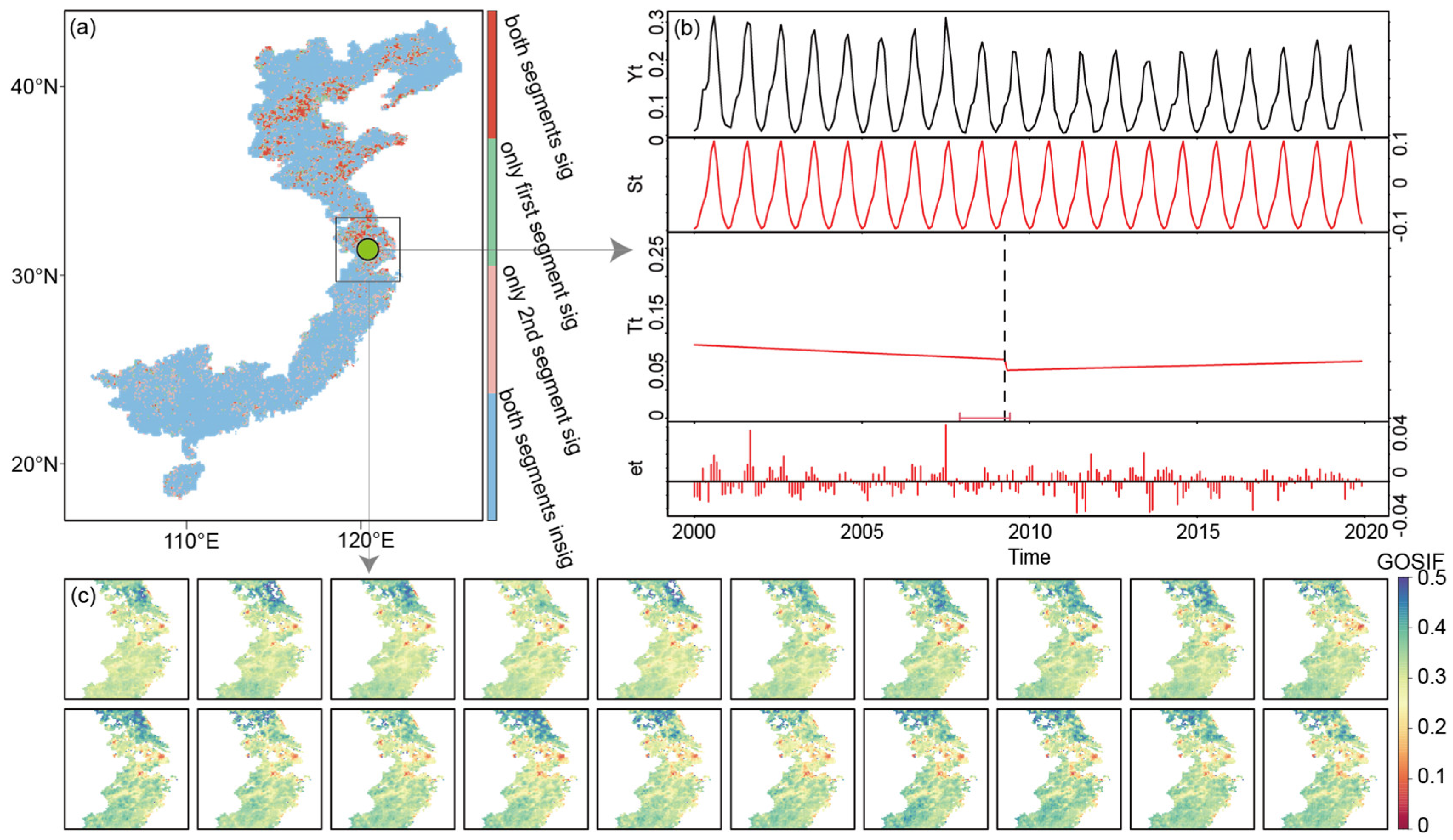
2.3.3. Abrupt Analysis

In this study, we applied the break for additive season and trend (BFAST) algorithm at the per-pixel level to monitor and describe significant changes (breakpoints) occurring in the vegetation time series. The BFAST algorithm utilizes an iterative approach to decompose time series into long-term trends, seasonal components, and residuals (as shown in Figure 2b). It characterizes vegetation features based on the direction and amplitude of breakpoints and is used for satellite time series analysis. This method can be directly applied to raw time series data without the need for additional standardization and predefined phenology trajectories [26]. Additionally, BFAST incorporates phenology harmonics models, making it effective for handling limited sample data with high accuracy when monitoring vegetation breakpoints at the pixel level [25]. The decomposition model is generally represented as

$${\mathrm{Y}}_{\mathrm{t}}={{\mathrm{S}}_{\mathrm{t}}+\mathrm{T}}_{\mathrm{t}}+{\mathrm{e}}_{\mathrm{t}}\left(\mathrm{t}=1,\dots ,\mathrm{n}\right)$$

(6)

Here, Y_t represents the observed data at time t, S_t represents the seasonal component, T_t represents the trend component, and e_t represents the residual component.

To detect the primary breakpoints in the SIF time series, we employed the BFAST method using the bfast01 function in R at the pixel level from 2000 to 2019. Following the categorization established by prior research [65], we classified changes in vegetation growth into six categories: “monotonic increase”, “monotonic decrease”, “increase with negative break”, “decrease with positive break”, “increase to decrease”, and “decrease to increase”. After categorizing the different combinations of two-segment changes following breakpoints, it is essential to note that the trend changes in individual segments may vary in significance. To better understand whether vegetation condition significantly changed over a single period, the study used four types to characterize the significance of different combinations of changes between two segments: (1) both segments were significant; (2) only the first segment was significant; (3) only the second segment was significant; and (4) neither segment was significant.

2.3.4. Time Lag-Accumulation Effects of Vegetation Responses to Climatic Factors

The time lag-accumulation effects of extreme climate on vegetation are characterized by calculating Pearson correlation coefficients. Extreme climate variables are treated as independent variables, while GOSIF, representing vegetation growth conditions, is the dependent variable. We assess their correlation at various time scales. Previous studies have shown that the monthly-scale lag-accumulation response of vegetation to climate is generally less than one-fourth of the year [39,43,45,66]. Therefore, we consider a time lag ranging from 0 to 3 months. Taking temperature as an example, the definition of lag-accumulation climate variables is as follows:

$${SIF}_t=\mathrm{b}\times {\sum }_{j=0}^k{TEM}_{t-i-j}+a$$

(7)

Here, a and b represent regression coefficients, while i and k can take values from 0 to 3. In this context, 0 means no time effect, and 1–3 represent one to three months of lag or accumulation. Different combinations of i and k allow for a comprehensive consideration of time effects. In Equation (7), four scenarios can be considered:

(i)

When i = 0 and k = 0, there is no time effect.

(ii)

When i = 0 and k is between 1 and 3, only time accumulation effects are considered.

(iii)

If i is between 1 and 3, and k = 0, only time lag effects are considered.

(iv)

When both i and k are between 1 and 3, both time lag and time accumulation effects are simultaneously considered, encompassing their combined effects. Therefore, the fourth scenario encompasses all possible time effects.

3. Result

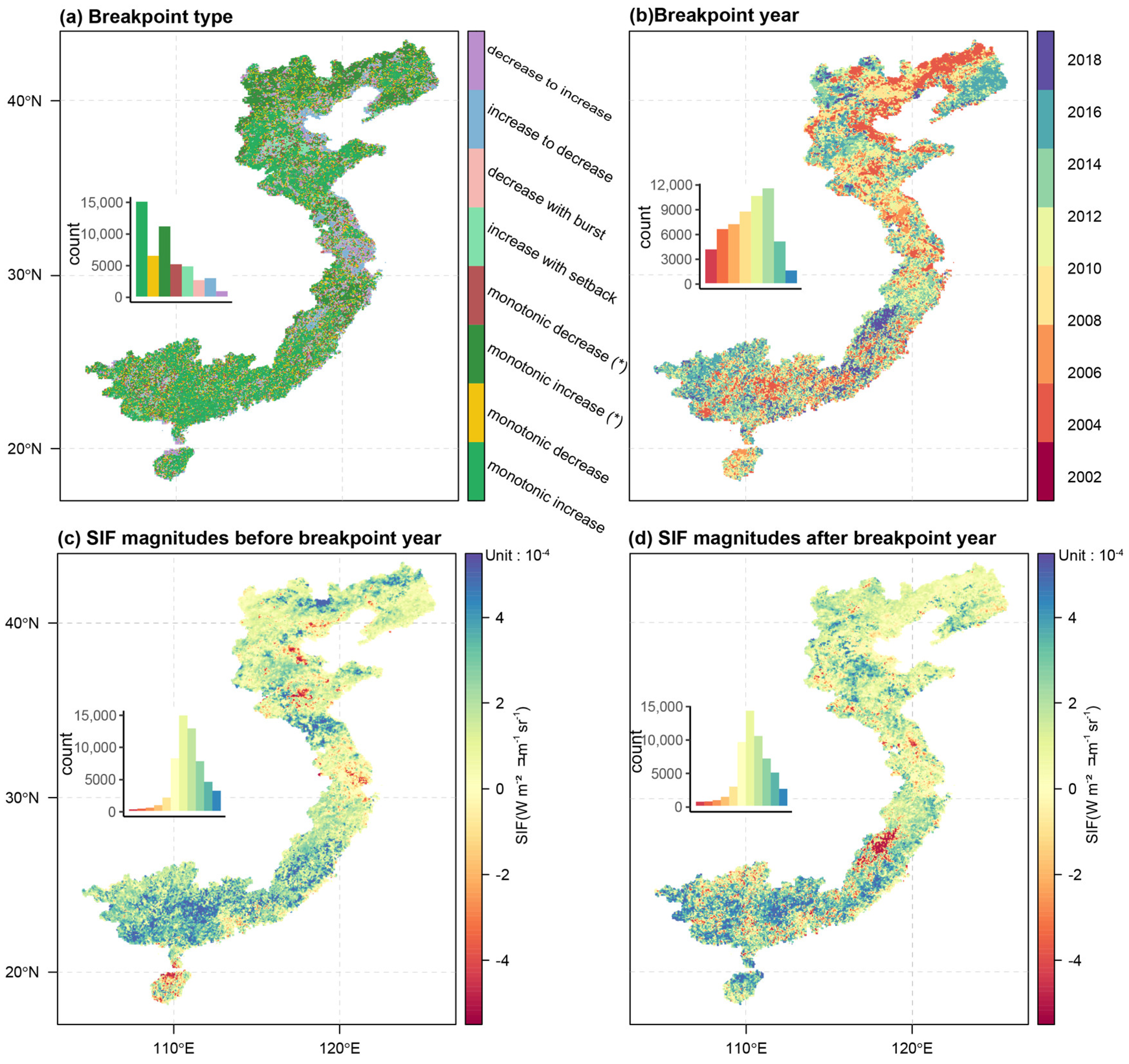
3.1. Gradual and Abrupt Vegetation Changes along the Coastal Areas of China

Mann–Kendall trend test and Sen’s slope analysis were employed to detect the vegetation gradual trends along the coastal areas of China (Figure 3). Despite a clear upward trend in most of the vegetation from 2000 to 2019, vegetation dynamics based on SIF exhibited significant spatial heterogeneity. In general, the northern part of the Chinese coast had a relatively gentle growth trend, the central region displayed localized spots of declining vegetation, especially in the Yangtze River estuary area, while the southern part exhibited the most noticeable improvement in vegetation, as clearly illustrated in Figure 3a. Combining trend analysis with significance test results, the coastal vegetation gradual trends were further categorized into five types, as illustrated in Figure 3b: “significant increase (sig+)”, “insignificant increase (insig+)”, “significant decrease (sig−)”, “insignificant decrease (insig−)”, and “stable”.

Based on this classification, the coastal regions showed a significant trend of vegetation improvement, with areas displaying an “increase” trend constituting 94.12% of the entire study area (60.01% of which exhibited a “significant increase”). Notably, the majority of “significant increase” was observed in the southern coastal areas. The areas with a “significant decrease” in SIF and those with an “insignificant decrease” accounted for 0.21% and 2.68%, respectively, both smaller in extent than the areas with SIF increases. Simultaneously, 2.99% of the region exhibited minimal changes in vegetation trends, remaining essentially “stable” (Figure 3b).

Vegetation dynamics can be exceptionally intense and intricate. Through the BFAST algorithm, we computed and assessed vegetation data along the Chinese coast from 2000 to 2019, resulting in spatial distribution diagrams illustrating various mutation trend types (Figure 4). The results show that the most common mutation type is “monotonic increase”, accounting for approximately 69.78% of the vegetation along the Chinese coast, with over 24.39% of this increase being statistically significant (Figure 4a). Conversely, the proportion of “monotonic decreases” was less than 2.35%, and the region with a “significant monotonic decrease” accounted for only 0.50%. Notably, there is a relatively high occurrence of “increase with negative break” (11.77%) and “increase to decrease” (9.48%) in the vegetation breakpoints along the Chinese coast. This indicates that the dynamics of coastal vegetation in China are not merely characterized by straightforward increases or decreases; the changes may be complex, varied, and characterized by fluctuation and complexity. Nonlinear trend detection results provide a clear classification of the various types, indicating substantial differences between them. Focusing solely on linear trend changes would not be sufficient to assess the variations in trend occurrences. Additionally, the most prevalent trend types are, in sequence, “monotonic increase”, “increase with negative break”, “increase to decrease”, and “decrease to increase”, underscoring the overall improvement in vegetation cover in most areas along the Chinese coast from 2000 to 2019. Nevertheless, there are also regions with a trend of vegetation decrease, highlighting the potential risk of vegetation degradation that should not be ignored.

As shown in Figure 4b, there is a certain regularity in the temporal distribution of vegetation trend mutations. Mutations occurred in different years, with the greatest concentration between 2010 and 2014 (Figure 4b). Corresponding to the mutation types, the years of mutation occurrence were generally earlier in the northern vegetation, mostly before 2010, and the main mutation types were monotonic increases, shifts from increase to decrease, and shifts from decrease to increase. In contrast, the southern vegetation experienced mutations predominantly after 2012, with the latest mutations occurring in Fujian Province, where most mutations concentrated after 2018, primarily characterized by monotonic increases.

The BFAST method revealed the magnitude of changes in the SIF time series before and after breakpoints. It is noteworthy that the fundamental SIF trend did not undergo a significant shift. Sustained growth remained the primary direction of change for coastal vegetation in China. Before the breakpoint, SIF in coastal vegetation increased at a rate of 2.19 × 10⁻⁴ W m⁻² μm⁻¹ sr⁻¹ month⁻¹. After the breakpoint, the growth rate decreased to 1.40 × 10⁻⁴ W m⁻² μm⁻¹ sr⁻¹ month⁻¹ (Figure 4c,d). Spatially, there are significant differences before and after the breakpoint. For instance, prior to the breakpoint, vegetation in Fujian Province showed a distinct upward trend, but after the breakpoint, it began to significantly decline. Before the breakpoint, approximately 86.97% of pixels in the study area exhibited a positive trend, with 10.87% of pixels having a growth rate greater than 5 × 10⁻⁴. The results indicate that before the breakpoint, most pixels exhibited positive trends, with only a small portion in the central coastal area showing negative trends. In the later period (post-breakpoint), the growing trend covered 78.72% of all pixels, with 6.84% of pixels having growth rates exceeding 5 × 10⁻⁴. The negative trend was randomly distributed, with no evident spatial clustering within the study area.

To elucidate the dynamic trends of vegetation in China’s coastal provinces over the past 20 years, we compared the results of gradual analysis and abrupt analysis. The outcomes of the gradual analysis were categorized into two classes: increase (including significant increase) and decrease (including significant decrease). Similarly, the results of the abrupt analysis were classified into three categories: increase (including significant increase), shift (including increase to decrease, decrease to increase, interrupted increase, interrupted decrease), and decrease (including significant decrease). The trend types from both methods were then overlaid. Among the outcomes indicating a decrease in gradual analysis, the proportions of decrease, shift, and increase in abrupt analysis were 46.09%, 52.65%, and 1.26%, respectively. Furthermore, the results indicated an increase in gradual analysis, while the proportions of decrease, shift, and increase in abrupt analysis were 1.01%, 25.40%, and 73.58%, respectively. Overall, while the results of gradual analysis and abrupt analysis are generally close, there are still certain differences. These differences arise from the additional trend types in abrupt analysis, including the increase to decrease, decrease to increase, interrupted increase, and interrupted decrease, which were not captured by gradual analysis. The appearance of these four abrupt types of vegetation growth may be attributed to the non-linear nature of climate change over the past 20 years, resulting in abrupt shifts. Additionally, human-induced disturbances, such as changes in land use, may have influenced vegetation changes, leading to various abrupt types in vegetation trends.

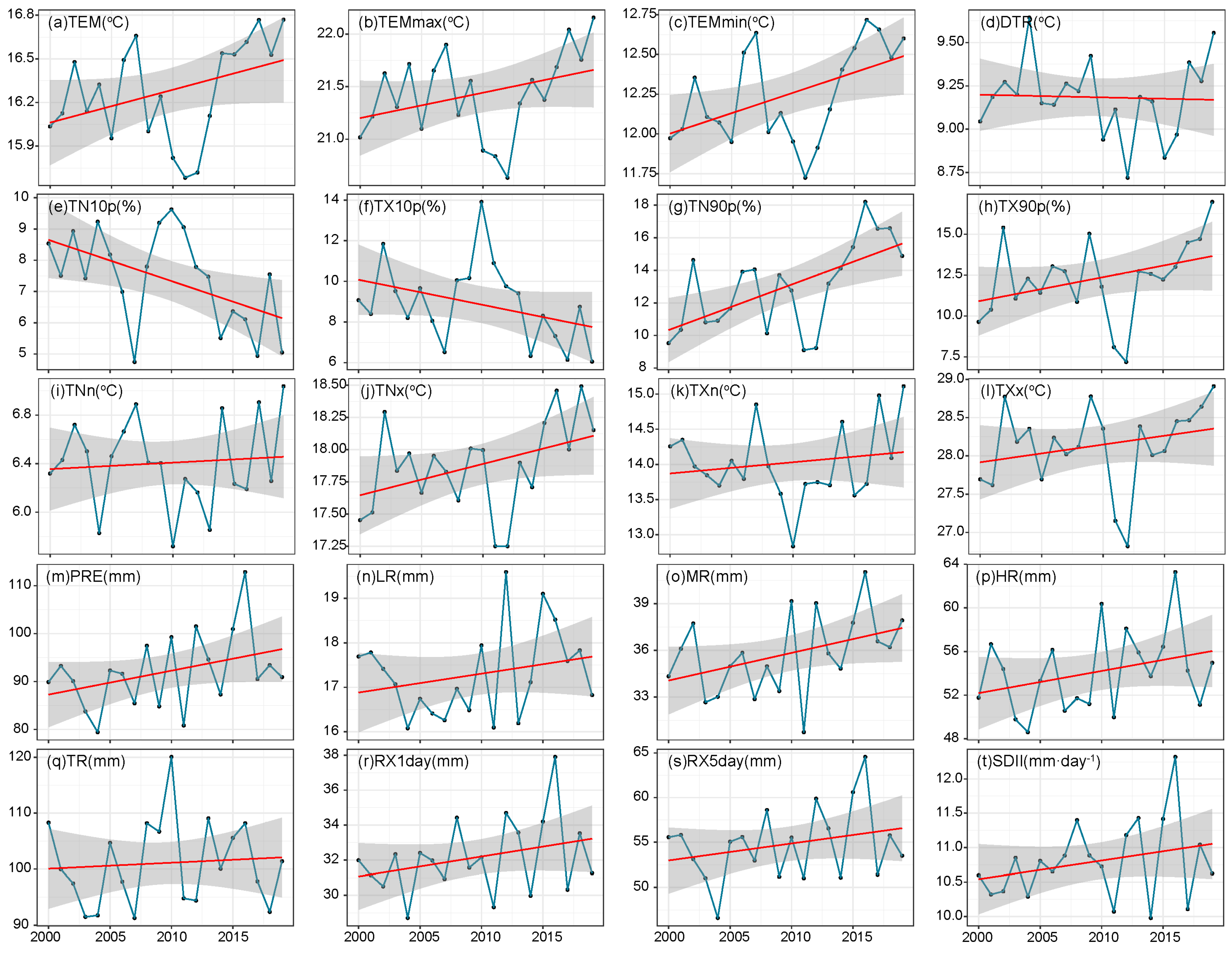
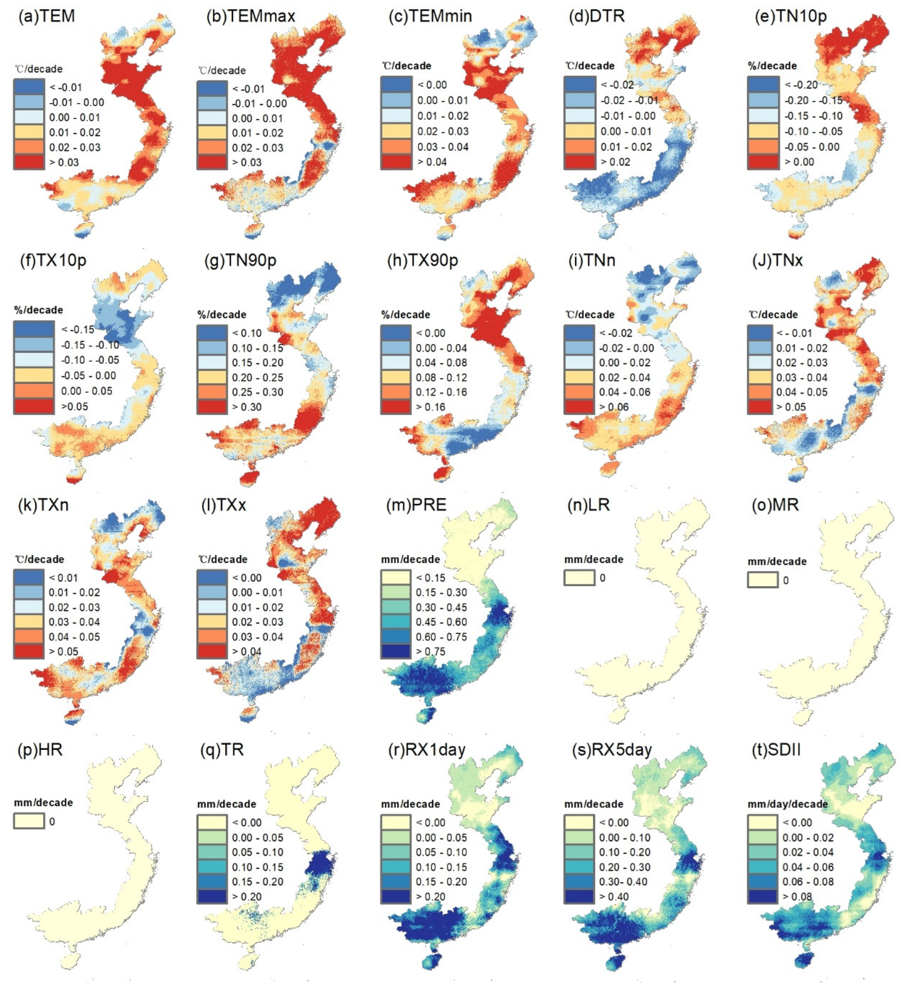
3.2. Temporal and Spatial Trends of Extreme Climate Indices

Based on data from 751 meteorological stations, monthly extreme climate indices for the past two decades in China’s coastal areas were extracted (Figure 5). Analysis reveals that among the extreme temperature indices, which represent temperature and extremely high temperatures, TEM, TEMmax, TEMmin, TN90p, TX90p, TNn, TNx, TXn, and TXx (Figure 5a–c,g–i) all show varying degrees of upward trends. Conversely, the indices representing extremely low temperatures, TN10p and TX10p (Figure 5e,f), display varying degrees of downward trends. Among them, TN90p, TEMmin, and TN10p displayed the most significant trends (p < 0.05), with trends of 2.793% per decade, 0.2567 °C per decade, and −1.317% per decade, respectively. The DTR index had the smallest amplitude of change, with a trend of only −0.01538 °C per decade. Nighttime warming was more pronounced than daytime warming, with the absolute values of the slopes for TN10p and TN90p exceeding those for Tx10p and Tx90p. Overall, the frequency of extreme events related to cold temperatures has significantly decreased, while the frequency of extreme events related to warm temperatures has greatly increased. Without a doubt, extreme temperature events in China’s coastal areas have significantly increased over the past two decades, consistent with the expected results of global warming. Indices representing extreme precipitation exhibited varying degrees of increasing trends (Figure 5m–t). Among them, the most significant change was observed in monthly precipitation, with a trend of 4.991 mm per decade. The rise in RX1day and RX5day indices also indirectly reflects that the increase in precipitation in China’s coastal areas may be concentrated in short periods of heavy and very heavy rainfall.

The spatial distribution of decadal trends in extreme climate indices along China’s coastal areas from 2000 to 2019 is shown in Figure 6. By analyzing temperature indices, we found that the regions with the largest increases in monthly average temperature, monthly high temperature, and monthly low temperature were mainly concentrated in the central and northern parts of China’s coastal region (Figure 6a–c). Among these, the Shandong, Jiangsu, and Fujian provinces exhibited the most significant temperature increases, with an overall rate exceeding 0.03 °C per decade. The diurnal temperature range (DTR) shows substantial spatial variations (Figure 6d), with a generally increasing trend in the north, where DTR rates are above 0.01 °C per decade, and a decreasing trend in the south, indicating an increase in day–night temperature differences in northern China, with a decrease in the southern region. Comparing the percentage of cold nights, TN10p (Figure 6e), and warm days, TX90p (Figure 6h), it was observed that the decrease in cold nights was more pronounced in the northern region, and the increase in warm days was significant. Conversely, comparing the percentage of cold days, TX10p (Figure 6f), and warm nights, TN90p (Figure 6g), revealed that the southern coastal provinces had more cold days and fewer warm nights. Similarly, the spatial distribution trends in the lowest daily minimum temperature (TNN) and the highest daily maximum temperature (TXX) (Figure 6i–l) corroborate these findings, with low points in the TNN curve indicating a smaller increase in the north and a greater increase in the south, while high points in the TXX curve exhibit the opposite trend overall, further confirming the opposing trends in day–night temperature variations between the northern and southern regions.

When examining precipitation indices (Figure 6m–q), the increase in precipitation is primarily concentrated in the southern areas, particularly around the Yangtze River estuary and the Guangdong-Guangxi region. Comparing the spatial characteristics of LR (light rain), MR (moderate rain), HR (heavy rain), and TR (total rain) along Chinese coastal areas, the increase in precipitation is mainly associated with the increase in very heavy rainfall (TR), while light, moderate, and heavy rains show no significant spatial changes. This finding is consistent with the trends observed in RX1day and RX5day. When analyzing the temporal and spatial trends of extreme precipitation, it is evident that the Yangtze River Delta and the Guangdong-Guangxi regions experience significant increases in very heavy rainfall. This suggests a potential risk of flooding and should be given close attention.

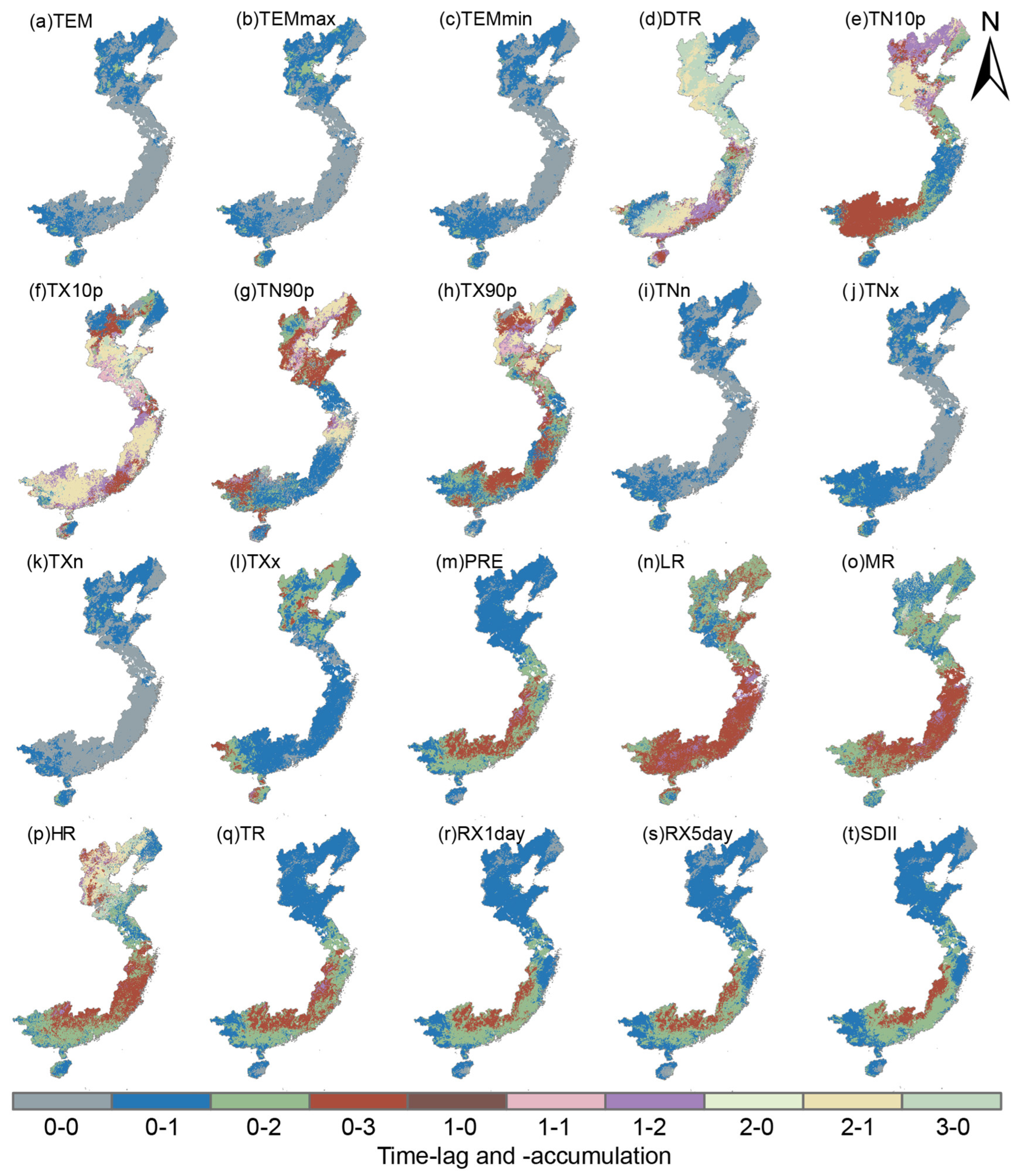
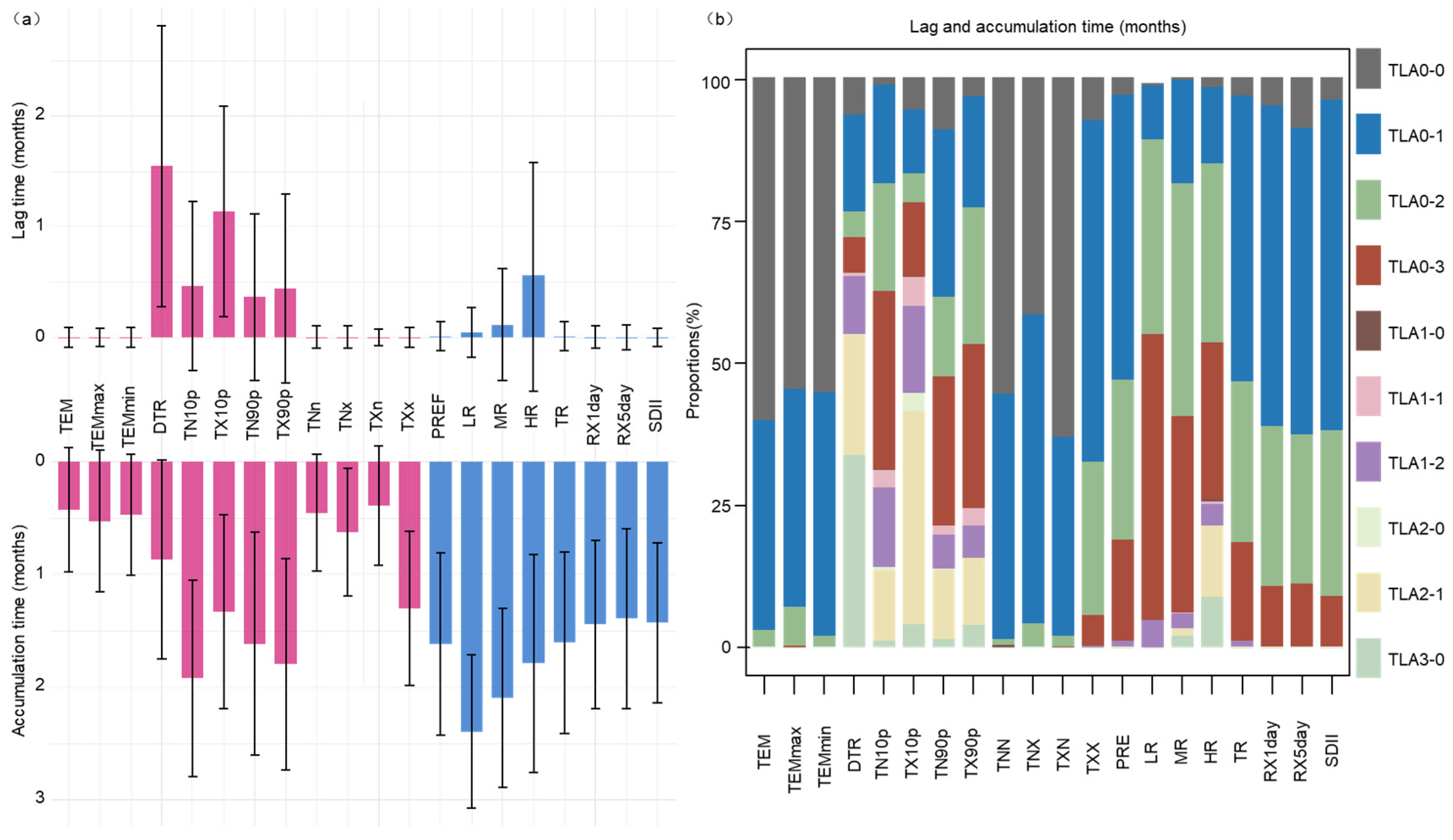
3.3. Time Lag-Accumulation Effects of Extreme Climate on Vegetation

Figure 7 displays the spatial patterns of climate variables with lag-accumulation months that influence the calculation of vegetation. Figure 8 and

Table 2. Mean values, standard deviations, and proportions of areas for different lag accumulation.

Climatic Indices	Mean Values and Standard Deviations		Proportions of Areas for Different Lag-Accumulation Times
	Lag	Accumulation	TLA0-0	TLA0-1	TLA0-2	TLA0-3	TLA1-0	TLA1-1	TLA1-2	TLA2-0	TLA2-1	TLA3-0
TEM	0.0027 ± 0.0893	0.4277 ± 0.5526	61.25	35.79	2.84	0.04	0.00	0.00	0.00	0.00	0.00	0.09
TEMmax	0.0022 ± 0.0811	0.5251 ± 0.6311	55.93	37.15	6.64	0.20	0.00	0.00	0.00	0.00	0.00	0.07
TEMmin	0.0027 ± 0.0904	0.4661 ± 0.5376	56.52	41.51	1.84	0.04	0.00	0.00	0.00	0.00	0.00	0.09
DTR	1.5455 ± 1.2681	0.8659 ± 0.8834	9.16	16.53	4.38	6.00	0.01	0.57	9.90	0.12	20.50	32.83
TN10p	0.4651 ± 0.7598	1.9218 ± 0.8738	4.07	16.80	18.35	30.42	0.09	2.95	13.60	0.71	11.89	1.12
TX10p	1.1385 ± 0.9464	1.3303 ± 0.8617	8.30	10.88	4.89	12.56	0.22	4.91	14.85	3.15	36.33	3.90
TN90p	0.3665 ± 0.7516	1.6149 ± 0.9875	11.59	28.62	13.55	25.42	0.05	1.48	5.83	0.26	11.83	1.36
TX90p	0.4420 ± 0.8489	1.7983 ± 0.9402	5.96	19.03	23.21	28.01	0.04	2.98	5.50	0.06	11.35	3.88
TNn	0.0057 ± 0.1007	0.4519 ± 0.5202	56.76	41.78	1.03	0.03	0.33	0.00	0.00	0.00	0.00	0.07
TNx	0.0034 ± 0.1006	0.6268 ± 0.5674	43.13	52.70	3.95	0.11	0.00	0.00	0.00	0.00	0.00	0.11
TXn	0.0018 ± 0.0732	0.3891 ± 0.5278	64.08	33.93	1.90	0.03	0.00	0.00	0.00	0.00	0.00	0.06
TXx	0.0047 ± 0.0906	1.3023 ± 0.6863	10.17	58.14	26.13	5.23	0.00	0.07	0.21	0.00	0.00	0.06
PREF	0.0128 ± 0.1298	1.6167 ± 0.8086	5.67	48.71	27.17	17.35	0.01	0.00	0.99	0.00	0.03	0.06
LR	0.0498 ± 0.2238	2.3987 ± 0.6819	4.18	9.21	33.20	48.72	0.00	0.00	4.61	0.01	0.03	0.03
MR	0.1166 ± 0.5052	2.0966 ± 0.7961	3.17	17.73	39.62	33.48	0.03	0.21	2.47	0.01	1.21	2.06
HR	0.5641 ± 1.0148	1.7889 ± 0.9679	4.49	12.95	30.56	26.66	0.40	0.51	3.58	0.07	12.16	8.62
TR	0.0131 ± 0.1294	1.6071 ± 0.8057	5.87	48.76	27.39	16.84	0.00	0.00	1.05	0.00	0.04	0.05
RX1day	0.0038 ± 0.0998	1.4442 ± 0.7478	7.55	54.63	27.33	10.34	0.01	0.00	0.01	0.00	0.04	0.08
RX5day	0.0047 ± 0.1117	1.3921 ± 0.7992	11.43	52.27	25.39	10.71	0.00	0.00	0.04	0.00	0.04	0.11
SDII	0.0024 ± 0.0790	1.4296 ± 0.7094	6.63	56.30	28.31	8.66	0.00	0.00	0.00	0.01	0.03	0.05

provide the mean values, standard deviations, and area proportions of different lag-accumulation months. The lag time for temperature indices (TEM, TEMmax, TEMmin, DTR, TN10p, TX10p, TN90p, TX90p, TNn, TNx, TXn, TXx) are 0.0027 ± 0.0893, 0.0022 ± 0.0811, 0.0027 ± 0.0904, 1.5455 ± 1.2681, 0.4651 ± 0.7598, 1.1385 ± 0.9464, 0.3665 ± 0.7516, 0.4420 ± 0.8489, 0.0057 ± 0.1007, 0.0034 ± 0.1006, 0.0018 ± 0.0732, and 0.0047 ± 0.0906 months, while the accumulation periods are 0.4277 ± 0.5526, 0.5251 ± 0.6311, 0.4661 ± 0.5376, 0.8659 ± 0.8834, 1.9218 ± 0.8738, 1.3303 ± 0.8617, 1.6149 ± 0.9875, 1.7983 ± 0.9402, 0.4519 ± 0.5202, 0.6268 ± 0.5674, 0.3891 ± 0.5278, and 1.3023 ± 0.6863 months. The combinations of lag-accumulation months for TEM, TEMmax, and TEMmin are the same, i.e., TLA0-0 and TLA0-1, with proportions of 61.25% and 35.79%(TEM), 55.93% and 37.15%(TEMmax), and 56.52% and 41.51%(TEMmin), respectively. This indicates that vegetation in Chinese coastal areas responds rapidly to temperature changes, typically producing positive feedback within the same month or the following month. The combinations that have the most significant impact on vegetation for TN90p and TX90p are mainly TLA0-3. This suggests that the increase in daytime and nighttime temperatures both exhibits a potentially longer positive feedback effect on vegetation. As for DTR, the primary combinations for lag-accumulation months are TLA2-1 and TLA3-0. DTR is the only temperature index where the proportion of lag effects is greater than the proportion of cumulative effects. Therefore, the cumulative effects of temperature on coastal vegetation in China tend to be more substantial than the lag effects in general.

Precipitation indices (PRE, LR, MR, HR, TR, RX1day, RX5day, SDII) have lag times of 0.0128 ± 0.1298, 0.0498 ± 0.2238, 0.1166 ± 0.5052, 0.5641 ± 1.0148, 0.0131 ± 0.1294, 0.0038 ± 0.0998, 0.0047 ± 0.1117, and 0.0024 ± 0.0790 months (mean ± standard deviation), and accumulation periods of 1.6167 ± 0.8086, 2.3987 ± 0.6819, 2.0966 ± 0.7961, 1.7889 ± 0.9679, 1.6071 ± 0.8057, 1.4442 ± 0.7478, 1.3921 ± 0.7992, and 1.4296 ± 0.7094 months, respectively. Among the eight precipitation indices, PRE, TR, RX1day, RX5day, and SDII predominantly exhibit the combinations of TLA0-1 (0 months lag and 1 month accumulation) and TLA0-2, accounting for 48.71% and 27.17% of the total vegetation grid cells (PRE), 48.76% and 27.39% (TR), 54.63% and 27.33% (RX1day), 52.27% and 25.39% (RX5day), and 56.30% and 28.31% (SDII). The remaining three indices, LR, MR, and HR, show mainly combinations of TLA0-2 and TLA0-3, with proportions of 33.20% and 48.72% (LR), 39.66% and 33.48% (MR), and 30.56% and 26.66% (HR). This indicates that the cumulative effects of light rain, moderate rain, and heavy rain on vegetation occur with a delay of approximately 2–3 months, which is slower than the extremely heavy rainfall (1–2 months). In summary, the time accumulation effects of precipitation indices are significant, while the lag effects are not significant. These results indicate that climate factors have both lag and cumulative effects on vegetation growth in the Chinese coastal region, thus supporting our hypothesis.

4. Discussion

4.1. Response of Climate Change in Chinese Coastal Areas to Global Changes

In the context of climate change, temperatures have been increasing in most parts of the world, with higher latitudes experiencing greater warming compared to lower latitudes [67,68]. Coastal China spans a wide range of latitudes, with significant zonal and regional variations in factors affecting plant growth, such as temperature, humidity, and surface substrates [53]. Overall, extreme high-temperature indices in the Chinese coastal region have been on the rise, while extreme temperature indices have been declining. Spatial differences in the trends of extreme precipitation indices are also observed, particularly in the area around the Yangtze River estuary and the Guangdong-Guangxi region, where extreme precipitation events are more frequent and intense. This implies an increased risk of flash floods, urban flooding, and landslides in these areas. Conversely, the northern parts of China are experiencing a decreasing trend in extreme precipitation, aligning with previous research on different regions of China [69,70,71,72].

Alexander et al. noted in global research on extreme climate change that 70% of the world’s land areas show a consistent decrease in cold nights and an increase in warm nights. In this study, we found that in the Chinese coastal region, nights are colder and days are hotter in the north [73]. Surprisingly, in the southern coastal provinces, there are more cold days and fewer warm nights, resulting in a conclusion opposite to the northern findings. The potential cause for this phenomenon might be the distinct atmospheric circulation zones between high and low latitudes. High-latitude regions are typically influenced by the polar jet stream and temperate climate zones, whereas low-latitude regions are influenced by tropical climate zones. Changes in these atmospheric circulation systems could result in opposite temperature trends in different regions.

It is worth noting that the warming trend in the Chinese coastal region may have various ecological and environmental impacts, including influencing phenological phenomena of vegetation, potentially disrupting ecological balances and species interactions, leading to shifts in ecological niches of vegetation, and affecting the distribution ranges of certain plant species [74,75]. It may also have significant implications for soil moisture and water resource distribution, subsequently impacting the water cycle. Additionally, the Chinese coastal region, as a transition zone between the ocean and inland areas, is profoundly affected by various large-scale climatic factors such as monsoons, atmospheric circulation, and ocean currents [76]. These factors have a profound impact on precipitation and its extreme events. The spatial heterogeneity of precipitation and the suddenness of extreme events will further exacerbate differences in extreme precipitation events between regions [77,78]. This poses challenges for urban planning and infrastructure development, especially in coastal cities.

4.2. Comparison of Gradual Analysis and Abrupt Analysis

Gradual analysis can reveal long-term trends in vegetation, identifying relatively stable changes. This is crucial for monitoring the health of ecosystems and assessing the long-term impacts of human or climatic factors on vegetation [25,65]. However, the gradual analysis does not provide information about specific time points and is unable to capture the nonlinear and non-stationary characteristics of vegetation time series induced by climate change and human activities, which limits its utility in understanding the impact of abrupt events [26,79,80]. In contrast, abrupt analysis (utilizing the BFAST algorithm) can reveal different types of changes and distinguish “when”, “where”, and “what type” breakpoints in a time series at a higher level of precision, rectifying the shortcomings of gradual analysis in vegetation monitoring [81,82]. This method is instrumental in determining the presence of certain abrupt events, such as extreme droughts, pest outbreaks, or abrupt vegetation changes due to human disturbances.

Based on this, we applied the pixel-based BFAST algorithm to detect dynamic vegetation breakpoints in the Chinese coastal region. Among the abrupt types in vegetation time series, the proportion of “monotonic increase” is the largest at 69.78%. This indicates that the Chinese coastal region has experienced an overall increase and partial degradation over the past 20 years. The overall increase may be attributed to the overall warming and humidification trend in the Chinese coastal region and the carbon fertilization effect resulting from the increase in atmospheric CO₂ concentration. The reasons for vegetation breakpoints in the Chinese coastal region are diverse and complex, involving both successional and disturbance-related factors. The increase in the southern coastal region is greater than that in the northern region, possibly due to a higher daytime biological accumulation rate in the south than in the north, while the nighttime temperature difference between the two regions is smaller, leading to similar nighttime respiration rates in the Chinese coastal region [83]. Areas with a “monotonic decrease” are concentrated in regions with significant urbanization pressure, such as the Yangtze River estuary, over the past few decades [84]. In general, before and after the breakpoints, the overall change in vegetation at the pixel level is improved (see Figure 4a), which aligns with the results of gradual analysis and confirms the findings of previous research by [54].

In conclusion, BFAST provides distinct advantages in monitoring extreme vegetation changes. It can detect subtle alterations caused by human activities, forest fires, and other factors that disrupt vegetation growth, which linear and Mann–Kendall tests cannot provide. In future analyses of spatiotemporal evolution, combining gradual analysis with abrupt analysis will help comprehensively understand vegetation changes, capture the multidimensional nature of vegetation dynamics, and assist scientists and policymakers in better comprehending how vegetation responds to external factors.

4.3. Temporal Effects of Extreme Climate on Coastal Chinese Vegetation

This study emphasizes the temporal effects of extreme climatic factors on vegetation. Different temperature and precipitation indices impact vegetation growth at various temporal scales, revealing the sensitivity of vegetation growth to climate change and its dynamic responses [37]. Vegetation can adapt to climate changes within its tolerance limits. However, when climate changes exceed critical thresholds, it can stress vegetation, leading to a halt in growth [85]. Therefore, climate effects on vegetation may exhibit temporal dynamics [86].

This study investigates the temporal effects of extreme climate on coastal vegetation in China at the pixel level. The results demonstrate that changes in coastal vegetation are not only influenced by current climate conditions but also by historical climate conditions (Figure 7 and Figure 8). Previous global vegetation dynamics studies suggest that vegetation response to temperature is mainly direct, consistent with our findings [43]. Temperature indices such as TEM, TEMmax, and TEMmin exhibit average lag-accumulation times of less than a month, indicating positive feedback to vegetation within the same or the following month (Figure 8). During the growing season, rising temperatures enhance photosynthetic efficiency and transpiration rates, leading to increased root water absorption [87].

In comparison to the direct impact of temperature on vegetation, precipitation’s impact appears much more gradual. Precipitation indices, such as PRE, TR, RX1day, RX5day, and SDII, display clear time accumulation effects, averaging 1–2 months. The accumulation effect of LR, MR, and TR is delayed compared to TR, taking approximately 2–3 months. These findings align with Ma et al.’s research in northern China. Moreover, this study reveals that the accumulation effect of precipitation in coastal China is greater than the lag effect, underscoring the substantial driving role of accumulated precipitation on vegetation growth in the study area. This phenomenon aligns with the research of [85] on the lag-accumulation effects of drought on grassland vegetation. Vegetation does not directly respond to precipitation but reacts to actual soil moisture [88]. The main reason is that when precipitation increases, the soil moisture is not immediately absorbed and utilized by vegetation, taking some time to penetrate to the root zones [89]. Additionally, deep soil moisture rising to the surface also requires time to sustain vegetation growth. When the amount of rainfall exceeds the plants’ utilization rate in a short time, the soil can retain a certain level of excess moisture, providing long-term nutrient supply to vegetation [90]. Furthermore, Ref. [91] study demonstrates that, regardless of climate zone and vegetation type, accumulation effects of precipitation are generally stronger than lag effects in most regions. This finding further corroborates that, relative to the immediate effectiveness of moisture at single time points within short periods, the accumulated effectiveness of moisture over specific time intervals has a more substantial impact on vegetation growth. Overall, we find that the cumulative effects of climate variables have a stronger explanatory power for vegetation growth than lag effects [92]. These results enhance our understanding of the relationship between climate and vegetation growth and offer valuable insights for vegetation management and climate change adaptation in the coastal regions of China.

4.4. Limitations and Uncertainty

While this study provides valuable insights into the relationship between vegetation and extreme climate events in the coastal regions of China, several limitations and uncertainties should be acknowledged. Firstly, although SIF data offer unique advantages in capturing evergreen forests compared to traditional vegetation indices, the data only cover the period from 2000 to 2019, which is a relatively short time frame. Longer-term data may be useful in better understanding patterns and trends in climate and vegetation changes. Therefore, future research could consider extending the time range to acquire more information.

Secondly, although we innovatively employed machine learning techniques combined with geographic spatial interpolation to interpolate extreme climate indices into spatial grids, greatly enhancing the accuracy of climate indices on a spatial scale, limitations still exist in regions with rugged terrain and sparse meteorological stations due to algorithmic variations.

Thirdly, different vegetation types exhibit specific resistance and adaptation mechanisms, allowing different vegetation types to respond rapidly to changes in climatic conditions [93]. Different vegetation types have varying mechanisms for the absorption and utilization of soil moisture, which may result in differences in the lag response to climate factors. This study does not account for the differential response of vegetation types to extreme climate events, which unavoidably affects the results. Further research into the distinct responses of various vegetation types is necessary to enhance clarity and reliability.

Lastly, the complex interactions between vegetation growth and extreme climate conditions may involve nonlinear relationships. Using simple correlation coefficient analyses for monthly-scale extreme climate indices and vegetation indices may overlook the impacts of seasonal variations, leading to uncertainties [94]. Therefore, gaining a better understanding of vegetation responses to climate change and elucidating the underlying mechanisms of extreme climate in vegetation time effects, while challenging, remains crucial.

5. Conclusions

This paper analyzes the spatiotemporal distribution patterns of climate indices, including extreme climate indices, and vegetation in China’s coastal regions over the past two decades. It clarifies the time lag and cumulative effects of vegetation in response to extreme climate events, leading to the following conclusions:

(1)

With an increase in the frequency of high-temperature events and extreme precipitation events, the northern coastal areas of China have experienced a gradual increase in day–night temperature differences, while the southern regions exhibit the opposite trend. Precipitation has primarily increased in the form of short-duration heavy rainfall, concentrated mainly in the Yangtze River Delta and the Guangdong-Guangxi region, with limited precipitation increase in the northern areas.

(2)

Gradual analysis and abrupt analysis reveal that the coastal regions of China have undergone overall improvement and partial degradation over the past two decades, with the southern regions showing more significant improvements in vegetation compared to the northern areas. Areas with more severe vegetation degradation are concentrated in regions facing rapid urbanization pressures, particularly in the Yangtze River estuary.

(3)

Vegetation’s response to temperature and precipitation indices exhibits a time lag-accumulation effect, with different indices producing varying feedback on vegetation growth at different time scales. Overall, cumulative effects of climate variables have a stronger explanatory power for vegetation growth in the coastal regions of China compared to lag effects. Specifically, vegetation responds more rapidly to temperature changes, typically within one month, while the response to precipitation becomes evident after a time accumulation of approximately 2–3 months. These results can enhance our understanding of the climate–vegetation relationship and are valuable for vegetation management and climate adaptation in the region.

References

1. Nesbitt, L.; Hotte, N.; Barron, S.; Cowan, J.; Sheppard, S.R.J. The social and economic value of cultural ecosystem services provided by urban forests in North America: A review and suggestions for future research. Urban For. Urban Green. 2017, 25, 103–111. [Google Scholar] [CrossRef]
2. Franklin, J.; Serra-Diaz, J.M.; Syphard, A.D.; Regan, H.M. Global change and terrestrial plant community dynamics. Proc. Natl. Acad. Sci. USA 2016, 113, 3725–3734. [Google Scholar] [CrossRef]
3. Piao, S.; Wang, X.; Wang, K.; Li, X.; Bastos, A.; Canadell, J.G.; Ciais, P.; Friedlingstein, P.; Sitch, S. Interannual variation of terrestrial carbon cycle: Issues and perspectives. Glob. Chang. Biol. 2020, 26, 300–318. [Google Scholar] [CrossRef] [PubMed]
4. Piao, S.; Wang, X.; Park, T.; Chen, C.; Lian, X.; He, Y.; Bjerke, J.W.; Chen, A.; Ciais, P.; Tømmervik, H.; et al. Characteristics, drivers and feedbacks of global greening. Nat. Rev. Earth Environ. 2020, 1, 14–27. [Google Scholar] [CrossRef]
5. Piao, S.; Liu, Q.; Chen, A.; Janssens, I.A.; Fu, Y.; Dai, J.; Liu, L.; Lian, X.; Shen, M.; Zhu, X. Plant phenology and global climate change: Current progresses and challenges. Glob. Chang. Biol. 2019, 25, 1922–1940. [Google Scholar] [CrossRef] [PubMed]
6. Wallace, J.M.; Held, I.M.; Thompson, D.W.; Trenberth, K.E.; Walsh, J.E. Global warming and winter weather. Science 2014, 343, 729–730. [Google Scholar] [CrossRef] [PubMed]
7. Xu, W.; Yuan, W.; Wu, D.; Zhang, Y.; Shen, R.; Xia, X.; Ciais, P.; Liu, J. Impacts of record-breaking compound heatwave and drought events in 2022 China on vegetation growth. Agric. For. Meteorol. 2024, 344, 109799. [Google Scholar] [CrossRef]
8. Tripathy, K.P.; Mishra, A.K. How Unusual Is the 2022 European Compound Drought and Heatwave Event? Geophys. Res. Lett. 2023, 50, e2023GL105453. [Google Scholar] [CrossRef]
9. Islam, A.; Islam, H.M.T.; Shahid, S.; Khatun, M.K.; Ali, M.M.; Rahman, M.S.; Ibrahim, S.M.; Almoajel, A.M. Spatiotemporal nexus between vegetation change and extreme climatic indices and their possible causes of change. J. Environ. Manag. 2021, 289, 112505. [Google Scholar] [CrossRef]
10. Zhou, Y.; Batelaan, O.; Guan, H.; Liu, T.; Duan, L.; Wang, Y.; Li, X. Assessing long-term trends in vegetation cover change in the Xilin River Basin: Potential for monitoring grassland degradation and restoration. J. Environ. Manag. 2024, 349, 119579. [Google Scholar] [CrossRef]
11. Smith, W.K.; Biederman, J.A.; Scott, R.L.; Moore, D.J.P.; He, M.; Kimball, J.S.; Yan, D.; Hudson, A.; Barnes, M.L.; MacBean, N.; et al. Chlorophyll Fluorescence Better Captures Seasonal and Interannual Gross Primary Productivity Dynamics across Dryland Ecosystems of Southwestern North America. Geophys. Res. Lett. 2018, 45, 748–757. [Google Scholar] [CrossRef]
12. Walther, S.; Voigt, M.; Thum, T.; Gonsamo, A.; Zhang, Y.; Köhler, P.; Jung, M.; Varlagin, A.; Guanter, L. Satellite chlorophyll fluorescence measurements reveal large-scale decoupling of photosynthesis and greenness dynamics in boreal evergreen forests. Glob. Chang. Biol. 2016, 22, 2979–2996. [Google Scholar] [CrossRef]
13. Wu, C.; Peng, D.; Soudani, K.; Siebicke, L.; Gough, C.M.; Arain, M.A.; Bohrer, G.; Lafleur, P.M.; Peichl, M.; Gonsamo, A.; et al. Land surface phenology derived from normalized difference vegetation index (NDVI) at global FLUXNET sites. Agric. For. Meteorol. 2017, 233, 171–182. [Google Scholar] [CrossRef]
14. Fang, J.; Lutz, J.A.; Wang, L.; Shugart, H.H.; Yan, X. Using climate-driven leaf phenology and growth to improve predictions of gross primary productivity in North American forests. Glob. Chang. Biol. 2020, 26, 6974–6988. [Google Scholar] [CrossRef] [PubMed]
15. Köehler, P.; Frankenberg, C.; Magney, T.S.; Guanter, L.; Joiner, J.; Landgraf, J. Global retrievals of solar induced chlorophyll fluorescence with TROPOMI: First results and inter-sensor comparison to OCO-2. Geophys. Res. Lett. 2018, 45, 10456–10463. [Google Scholar] [CrossRef] [PubMed]
16. Li, X.; Xiao, J.; He, B.; Altaf Arain, M.; Beringer, J.; Desai, A.R.; Emmel, C.; Hollinger, D.Y.; Krasnova, A.; Mammarella, I.; et al. Solar-induced chlorophyll fluorescence is strongly correlated with terrestrial photosynthesis for a wide variety of biomes: First global analysis based on OCO-2 and flux tower observations. Glob. Chang. Biol. 2018, 24, 3990–4008. [Google Scholar] [CrossRef] [PubMed]
17. Frankenberg, C.; O’Dell, C.; Berry, J.; Guanter, L.; Joiner, J.; Köhler, P.; Pollock, R.; Taylor, T.E. Prospects for chlorophyll fluorescence remote sensing from the Orbiting Carbon Observatory-2. Remote Sens. Environ. 2014, 147, 1–12. [Google Scholar] [CrossRef]
18. Sun, Y.; Fu, R.; Dickinson, R.; Joiner, J.; Frankenberg, C.; Gu, L.; Xia, Y.; Fernando, N. Drought onset mechanisms revealed by satellite solar-induced chlorophyll fluorescence: Insights from two contrasting extreme events. J. Geophys. Res. Biogeosci. 2015, 120, 2427–2440. [Google Scholar] [CrossRef]
19. Wang, S.; Huang, C.; Zhang, L.; Lin, Y.; Cen, Y.; Wu, T. Monitoring and Assessing the 2012 Drought in the Great Plains: Analyzing Satellite-Retrieved Solar-Induced Chlorophyll Fluorescence, Drought Indices, and Gross Primary Production. Remote Sens. 2016, 8, 61. [Google Scholar] [CrossRef]
20. He, P.; Sun, Z.; Xu, D.; Liu, H.; Yao, R.; Ma, J. Combining gradual and abrupt analysis to detect variation of vegetation greenness on the loess areas of China. Front. Earth Sci. 2022, 16, 368–380. [Google Scholar] [CrossRef]
21. He, P.; Sun, Z.; Han, Z.; Dong, Y.; Liu, H.; Meng, X.; Ma, J. Dynamic characteristics and driving factors of vegetation greenness under changing environments in Xinjiang, China. Environ. Sci. Pollut. Res. Int. 2021, 28, 42516–42532. [Google Scholar] [CrossRef] [PubMed]
22. Marengo, J.A.; Espinoza, J.C. Extreme seasonal droughts and floods in Amazonia: Causes, trends and impacts. Int. J. Climatol. 2015, 36, 1033–1050. [Google Scholar] [CrossRef]
23. Ummenhofer, C.C.; Meehl, G.A. Extreme weather and climate events with ecological relevance: A review. Philos. Trans. R. Soc. Lond. B Biol. Sci. 2017, 372, 20160135. [Google Scholar] [CrossRef] [PubMed]
24. Pan, N.; Feng, X.; Fu, B.; Wang, S.; Ji, F.; Pan, S. Increasing global vegetation browning hidden in overall vegetation greening: Insights from time-varying trends. Remote Sens. Environ. 2018, 214, 59–72. [Google Scholar] [CrossRef]
25. Verbesselt, J.; Hyndman, R.; Newnham, G.; Culvenor, D. Detecting trend and seasonal changes in satellite image time series. Remote Sens. Environ. 2010, 114, 106–115. [Google Scholar] [CrossRef]
26. Verbesselt, J.; Zeileis, A.; Herold, M. Near real-time disturbance detection using satellite image time series. Remote Sens. Environ. 2012, 123, 98–108. [Google Scholar] [CrossRef]
27. Richardson, A.D.; Keenan, T.F.; Migliavacca, M.; Ryu, Y.; Sonnentag, O.; Toomey, M. Climate change, phenology, and phenological control of vegetation feedbacks to the climate system. Agric. For. Meteorol. 2013, 169, 156–173. [Google Scholar] [CrossRef]
28. Thuiller, W.; Lavorel, S.; Araújo, M.B.; Sykes, M.T.; Prentice, I.C. Climate change threats to plant diversity in Europe. Proc. Natl. Acad. Sci. USA 2005, 102, 8245–8250. [Google Scholar] [CrossRef]
29. Zhao, J.; Huang, S.; Huang, Q.; Wang, H.; Leng, G.; Fang, W. Time-lagged response of vegetation dynamics to climatic and teleconnection factors. Catena 2020, 189, 104474. [Google Scholar] [CrossRef]
30. Li, C.; Wang, R.; Ning, H.; Luo, Q. Changes in climate extremes and their impact on wheat yield in Tianshan Mountains region, northwest China. Environ. Earth Sci. 2016, 75, 1228. [Google Scholar] [CrossRef]
31. Xu, C.; McDowell, N.G.; Fisher, R.A.; Wei, L.; Sevanto, S.; Christoffersen, B.O.; Weng, E.; Middleton, R.S. Increasing impacts of extreme droughts on vegetation productivity under climate change. Nat. Clim. Chang. 2019, 9, 948–953. [Google Scholar] [CrossRef]
32. Tan, Z.; Tao, H.; Jiang, J.; Zhang, Q. Influences of Climate Extremes on NDVI (Normalized Difference Vegetation Index) in the Poyang Lake Basin, China. Wetlands 2015, 35, 1033–1042. [Google Scholar] [CrossRef]
33. Ying, H.; Zhang, H.; Zhao, J.; Shan, Y.; Zhang, Z.; Guo, X.; Rihan, W.; Deng, G. Effects of spring and summer extreme climate events on the autumn phenology of different vegetation types of Inner Mongolia, China, from 1982 to 2015. Ecol. Indic. 2020, 111, 105974. [Google Scholar] [CrossRef]
34. Li, C.; Wang, J.; Hu, R.; Yin, S.; Bao, Y.; Ayal, D.Y. Relationship between vegetation change and extreme climate indices on the Inner Mongolia Plateau, China, from 1982 to 2013. Ecol. Indic. 2018, 89, 101–109. [Google Scholar] [CrossRef]
35. Luo, M.; Sa, C.; Meng, F.; Duan, Y.; Liu, T.; Bao, Y. Assessing extreme climatic changes on a monthly scale and their implications for vegetation in Central Asia. J. Clean. Prod. 2020, 271, 122396. [Google Scholar] [CrossRef]
36. Jiang, H.; Xu, X. Impact of extreme climates on vegetation from multiple scales and perspectives in the Agro-pastural Transitional Zone of Northern China in the past three decades. J. Clean. Prod. 2022, 372, 133459. [Google Scholar] [CrossRef]
37. Ma, Y.; Guan, Q.; Sun, Y.; Zhang, J.; Yang, L.; Yang, E.; Li, H.; Du, Q. Three-dimensional dynamic characteristics of vegetation and its response to climatic factors in the Qilian Mountains. Catena 2022, 208, 105694. [Google Scholar] [CrossRef]
38. Wen, Y.; Liu, X.; Pei, F.; Li, X.; Du, G. Non-uniform time-lag effects of terrestrial vegetation responses to asymmetric warming. Agric. For. Meteorol. 2018, 252, 130–143. [Google Scholar] [CrossRef]
39. Chen, T.; de Jeu, R.A.M.; Liu, Y.Y.; van der Werf, G.R.; Dolman, A.J. Using satellite based soil moisture to quantify the water driven variability in NDVI: A case study over mainland Australia. Remote Sens. Environ. 2014, 140, 330–338. [Google Scholar] [CrossRef]
40. Vicente-Serrano, S.M.; Gouveia, C.; Camarero, J.J.; Beguería, S.; Trigo, R.; López-Moreno, J.I.; Azorín-Molina, C.; Pasho, E.; Lorenzo-Lacruz, J.; Revuelto, J.; et al. Response of vegetation to drought time-scales across global land biomes. Proc. Natl. Acad. Sci. USA 2013, 110, 52–57. [Google Scholar] [CrossRef]
41. Anderson, L.O.; Malhi, Y.; Aragão, L.E.; Ladle, R.; Arai, E.; Barbier, N.; Phillips, O. Remote sensing detection of droughts in Amazonian forest canopies. New Phytol. 2010, 187, 733–750. [Google Scholar] [CrossRef] [PubMed]
42. Bunting, E.L.; Munson, S.M.; Villarreal, M.L. Climate legacy and lag effects on dryland plant communities in the southwestern U.S. Ecol. Indic. 2017, 74, 216–229. [Google Scholar] [CrossRef]
43. Wu, D.; Zhao, X.; Liang, S.; Zhou, T.; Huang, K.; Tang, B.; Zhao, W. Time-lag effects of global vegetation responses to climate change. Glob. Chang. Biol. 2015, 21, 3520–3531. [Google Scholar] [CrossRef] [PubMed]
44. Wen, Y.; Liu, X.; Yang, J.; Lin, K.; Du, G. NDVI indicated inter-seasonal non-uniform time-lag responses of terrestrial vegetation growth to daily maximum and minimum temperature. Glob. Planet. Chang. 2019, 177, 27–38. [Google Scholar] [CrossRef]
45. Ding, Y.; Li, Z.; Peng, S. Global analysis of time-lag and -accumulation effects of climate on vegetation growth. Int. J. Appl. Earth Obs. Geoinf. 2020, 92, 102179. [Google Scholar] [CrossRef]
46. Liu, H.; Zhang, A.; Liu, C.; Zhao, Y.; Zhao, A.; Wang, D. Analysis of the time-lag effects of climate factors on grassland productivity in Inner Mongolia. Glob. Ecol. Conserv. 2021, 30, e01751. [Google Scholar] [CrossRef]
47. Wei, W.; Liu, T.; Zhou, L.; Wang, J.; Yan, P.; Xie, B.; Zhou, J. Drought-Related Spatiotemporal Cumulative and Time-Lag Effects on Terrestrial Vegetation across China. Remote Sens. 2023, 15, 4362. [Google Scholar] [CrossRef]
48. Zhe, M.; Zhang, X. Time-lag effects of NDVI responses to climate change in the Yamzhog Yumco Basin, South Tibet. Ecol. Indic. 2021, 124, 107431. [Google Scholar] [CrossRef]
49. Liu, L.; Zheng, J.; Guan, J.; Han, W.; Liu, Y. Grassland cover dynamics and their relationship with climatic factors in China from 1982 to 2021. Sci. Total Environ. 2023, 905, 167067. [Google Scholar] [CrossRef]
50. Rammig, A.; Wiedermann, M.; Donges, J.F.; Babst, F.; von Bloh, W.; Frank, D.; Thonicke, K.; Mahecha, M.D. Coincidences of climate extremes and anomalous vegetation responses: Comparing tree ring patterns to simulated productivity. Biogeosciences 2015, 12, 373–385. [Google Scholar] [CrossRef]
51. Liu, C.; Yang, M.; Hou, Y.; Xue, X. Ecosystem service multifunctionality assessment and coupling coordination analysis with land use and land cover change in China’s coastal zones. Sci. Total Environ. 2021, 797, 149033. [Google Scholar] [CrossRef]
52. Meng, Z.; Liu, M.; Gao, C.; Zhang, Y.; She, Q.; Long, L.; Tu, Y.; Yang, Y. Greening and browning of the coastal areas in mainland China: Spatial heterogeneity, seasonal variation and its influential factors. Ecol. Indic. 2020, 110, 105888. [Google Scholar] [CrossRef]
53. Wang, X.; Hou, X.; Wang, Y. Spatiotemporal variations and regional differences of extreme precipitation events in the Coastal area of China from 1961 to 2014. Atmos. Res. 2017, 197, 94–104. [Google Scholar] [CrossRef]
54. Xu, X.; Jiang, H.; Guan, M.; Wang, L.; Huang, Y.; Jiang, Y.; Wang, A. Vegetation responses to extreme climatic indices in coastal China from 1986 to 2015. Sci. Total Environ. 2020, 744, 140784. [Google Scholar] [CrossRef]
55. Li, X.; Xiao, J. Mapping Photosynthesis Solely from Solar-Induced Chlorophyll Fluorescence: A Global, Fine-Resolution Dataset of Gross Primary Production Derived from OCO-2. Remote Sens. 2019, 11, 2563. [Google Scholar] [CrossRef]
56. Li, X.; Xiao, J.; Kimball, J.S.; Reichle, R.H.; Scott, R.L.; Litvak, M.E.; Bohrer, G.; Frankenberg, C. Synergistic use of SMAP and OCO-2 data in assessing the responses of ecosystem productivity to the 2018 U.S. drought. Remote Sens. Environ. 2020, 251, 112062. [Google Scholar] [CrossRef]
57. Yao, T.; Liu, S.; Hu, S.; Mo, X. Response of vegetation ecosystems to flash drought with solar-induced chlorophyll fluorescence over the Hai River Basin, China during 2001–2019. J. Environ. Manag. 2022, 313, 114947. [Google Scholar] [CrossRef] [PubMed]
58. Zhang, Y.; Ye, A. Would the obtainable gross primary productivity (GPP) products stand up? A critical assessment of 45 global GPP products. Sci. Total Environ. 2021, 783, 146965. [Google Scholar] [CrossRef] [PubMed]
59. Dong, T.; Liu, J.; Liu, D.; He, P.; Li, Z.; Shi, M.; Xu, J. Spatiotemporal variability characteristics of extreme climate events in Xinjiang during 1960–2019. Environ. Sci. Pollut. Res. Int. 2023, 30, 57316–57330. [Google Scholar] [CrossRef] [PubMed]
60. Huang, C.; Feng, J.; Tang, F.; He, H.S.; Liang, Y.; Wu, M.M.; Xu, W.; Liu, B.; Shi, F.; Chen, F. Predicting the responses of boreal forests to climate-fire-vegetation interactions in Northeast China. Environ. Model. Softw. 2022, 153, 105410. [Google Scholar] [CrossRef]
61. Gong, H.; Cheng, Q.; Jin, H.; Ren, Y. Effects of temporal, spatial, and elevational variation in bioclimatic indices on the NDVI of different vegetation types in Southwest China. Ecol. Indic. 2023, 154, 110499. [Google Scholar] [CrossRef]
62. Varón-Ramírez, V.M.; Araujo-Carrillo, G.A.; Guevara Santamaría, M.A. Colombian soil texture: Building a spatial ensemble model. Earth Syst. Sci. Data 2022, 14, 4719–4741. [Google Scholar] [CrossRef]
63. Sen, P.K. Estimates of the Regression Coefficient Based on Kendall’s Tau. J. Am. Stat. Assoc. 1968, 63, 1379–1389. [Google Scholar] [CrossRef]
64. Juhl, T.; Xiao, Z. A nonparametric test for changing trends. J. Econom. 2005, 127, 179–199. [Google Scholar] [CrossRef]
65. De Jong, R.; Verbesselt, J.; Zeileis, A.; Schaepman, M.E. Shifts in Global Vegetation Activity Trends. Remote Sens. 2013, 5, 1117–1133. [Google Scholar] [CrossRef]
66. Ning, T.; Liu, W.; Lin, W.; Song, X. NDVI Variation and Its Responses to Climate Change on the Northern Loess Plateau of China from 1998 to 2012. Adv. Meteorol. 2015, 2015, 725427. [Google Scholar] [CrossRef]
67. Intergovernmental Panel on Climate Change. Climate Change 2014—Impacts, Adaptation and Vulnerability: Part B: Regional Aspects: Working Group II Contribution to the IPCC Fifth Assessment Report: Volume 2: Regional Aspects; Cambridge University Press: Cambridge, UK, 2014; Volume 2. [Google Scholar]
68. Intergovernmental Panel on Climate Change. Climate Change 2013—The Physical Science Basis: Working Group I Contribution to the Fifth Assessment Report of the Intergovernmental Panel on Climate Change; Cambridge University Press: Cambridge, UK, 2014. [Google Scholar]
69. Guo, E.; Zhang, J.; Wang, Y.; Quan, L.; Zhang, R.; Zhang, F.; Zhou, M. Spatiotemporal variations of extreme climate events in Northeast China during 1960–2014. Ecol. Indic. 2019, 96, 669–683. [Google Scholar] [CrossRef]
70. Li, X.; Zhang, K.; Bao, H.; Zhang, H. Climatology and changes in hourly precipitation extremes over China during 1970–2018. Sci. Total Environ. 2022, 839, 156297. [Google Scholar] [CrossRef]
71. You, Q.; Kang, S.; Aguilar, E.; Pepin, N.; Flügel, W.-A.; Yan, Y.; Xu, Y.; Zhang, Y.; Huang, J. Changes in daily climate extremes in China and their connection to the large scale atmospheric circulation during 1961–2003. Clim. Dyn. 2011, 36, 2399–2417. [Google Scholar] [CrossRef]
72. Zhao, Y.; Zou, X.; Cao, L.; Xu, X. Changes in precipitation extremes over the Pearl River Basin, southern China, during 1960–2012. Quat. Int. 2014, 333, 26–39. [Google Scholar] [CrossRef]
73. Alexander, L.V.; Zhang, X.; Peterson, T.C.; Caesar, J.; Gleason, B.; Klein Tank, A.M.G.; Haylock, M.; Collins, D.; Trewin, B.; Rahimzadeh, F.; et al. Global observed changes in daily climate extremes of temperature and precipitation. J. Geophys. Res. Atmos. 2006, 111, 1042–1063. [Google Scholar] [CrossRef]
74. Wang, L.; De Boeck, H.J.; Chen, L.; Song, C.; Chen, Z.; McNulty, S.; Zhang, Z. Urban warming increases the temperature sensitivity of spring vegetation phenology at 292 cities across China. Sci. Total Environ. 2022, 834, 155154. [Google Scholar] [CrossRef]
75. Rahman, I.U.; Hart, R.E.; Afzal, A.; Iqbal, Z.; Bussmann, R.W.; Ijaz, F.; Khan, M.A.; Ali, H.; Rahman, S.U.; Hashem, A.; et al. Vegetation-environment interactions: Plant species distribution and community assembly in mixed coniferous forests of Northwestern Himalayas. Sci. Rep. 2023, 13, 17228. [Google Scholar] [CrossRef]
76. Ding, Y.; Wang, Z.; Sun, Y. Inter-decadal variation of the summer precipitation in East China and its association with decreasing Asian summer monsoon. Part I: Observed evidences. Int. J. Climatol. 2008, 28, 1139–1161. [Google Scholar] [CrossRef]
77. Tammets, T.; Jaagus, J. Climatology of precipitation extremes in Estonia using the method of moving precipitation totals. Theor. Appl. Climatol. 2013, 111, 623–639. [Google Scholar] [CrossRef]
78. Sura, P. A general perspective of extreme events in weather and climate. Atmos. Res. 2011, 101, 1–21. [Google Scholar] [CrossRef]
79. Gholamnia, M.; Khandan, R.; Bonafoni, S.; Sadeghi, A. Spatiotemporal Analysis of MODIS NDVI in the Semi-Arid Region of Kurdistan (Iran). Remote Sens. 2019, 11, 1723. [Google Scholar] [CrossRef]
80. Verbesselt, J.; Hyndman, R.; Zeileis, A.; Culvenor, D. Phenological change detection while accounting for abrupt and gradual trends in satellite image time series. Remote Sens. Environ. 2010, 114, 2970–2980. [Google Scholar] [CrossRef]
81. Tong, X.; Brandt, M.; Yue, Y.; Horion, S.; Wang, K.; Keersmaecker, W.D.; Tian, F.; Schurgers, G.; Xiao, X.; Luo, Y.; et al. Increased vegetation growth and carbon stock in China karst via ecological engineering. Nat. Sustain. 2018, 1, 44–50. [Google Scholar] [CrossRef]
82. Niu, Q.; Xiao, X.; Zhang, Y.; Qin, Y.; Dang, X.; Wang, J.; Zou, Z.; Doughty, R.B.; Brandt, M.; Tong, X.; et al. Ecological engineering projects increased vegetation cover, production, and biomass in semiarid and subhumid Northern China. Land Degrad. Dev. 2019, 30, 1620–1631. [Google Scholar] [CrossRef]
83. Wang, X.; Wang, M.T.; Feng, Y.; Zou, Y.J.; Guo, B. Variation characteristics of normalized difference vegetation index in Northwestern Sichuan Plateau and its response to extreme climate during 2001–2020. Ying Yong Sheng Tai Xue Bao 2022, 33, 1957–1965. [Google Scholar] [CrossRef] [PubMed]
84. Xiong, Y.; Peng, F.; Zou, B. Spatiotemporal influences of land use/cover changes on the heat island effect in rapid urbanization area. Front. Earth Sci. 2019, 13, 614–627. [Google Scholar] [CrossRef]
85. Zhao, A.; Yu, Q.; Feng, L.; Zhang, A.; Pei, T. Evaluating the cumulative and time-lag effects of drought on grassland vegetation: A case study in the Chinese Loess Plateau. J. Environ. Manag. 2020, 261, 110214. [Google Scholar] [CrossRef] [PubMed]
86. Yamori, W.; Hikosaka, K.; Way, D.A. Temperature response of photosynthesis in C3, C4, and CAM plants: Temperature acclimation and temperature adaptation. Photosynth. Res. 2014, 119, 101–117. [Google Scholar] [CrossRef] [PubMed]
87. Querejeta, J.I.; Ren, W.; Prieto, I. Vertical decoupling of soil nutrients and water under climate warming reduces plant cumulative nutrient uptake, water-use efficiency and productivity. New Phytol. 2021, 230, 1378–1393. [Google Scholar] [CrossRef] [PubMed]
88. Paudel, K.P.; Andersen, P. Response of rangeland vegetation to snow cover dynamics in Nepal Trans Himalaya. Clim. Chang. 2013, 117, 149–162. [Google Scholar] [CrossRef]
89. Vicente-Serrano, S.M.; Camarero, J.J.; Azorin-Molina, C. Diverse responses of forest growth to drought time-scales in the Northern Hemisphere. Glob. Ecol. Biogeogr. 2014, 23, 1019–1030. [Google Scholar] [CrossRef]
90. Zhang, Y.; Liang, S. Changes in forest biomass and linkage to climate and forest disturbances over Northeastern China. Glob. Chang. Biol. 2014, 20, 2596–2606. [Google Scholar] [CrossRef]
91. Wei, X.; He, W.; Zhou, Y.; Ju, W.; Xiao, J.; Li, X.; Liu, Y.; Xu, S.; Bi, W.; Zhang, X.; et al. Global assessment of lagged and cumulative effects of drought on grassland gross primary production. Ecol. Indic. 2022, 136, 108646. [Google Scholar] [CrossRef]
92. Jiang, W.; Niu, Z.; Wang, L.; Yao, R.; Gui, X.; Xiang, F.; Ji, Y. Impacts of Drought and Climatic Factors on Vegetation Dynamics in the Yellow River Basin and Yangtze River Basin, China. Remote Sens. 2022, 14, 930. [Google Scholar] [CrossRef]
93. Liu, L.; Peng, J.; Li, G.; Guan, J.; Han, W.; Ju, X.; Zheng, J. Effects of drought and climate factors on vegetation dynamics in Central Asia from 1982 to 2020. J. Environ. Manag. 2023, 328, 116997. [Google Scholar] [CrossRef]
94. Ma, M.; Wang, Q.; Liu, R.; Zhao, Y.; Zhang, D. Effects of climate change and human activities on vegetation coverage change in northern China considering extreme climate and time-lag and -accumulation effects. Sci. Total Environ. 2023, 860, 160527. [Google Scholar] [CrossRef]
Figure 1. (a) Background information of coastal China. (b) Distribution map of meteorological stations. (c) Multi-year average SIF distribution map.
Remotesensing 16 00528 g001
Figure 2. A case study verifies the effectiveness of the BFAST algorithm for monitoring the breakpoint on the time series. (a) BFAST method detected the stability on the pixel scale over coastal China. The green spots in the map represent the pixels selected to verify the effectiveness of the BFAST algorithm. (b) BFAST algorithm was used to decompose the three variables in the time series. Yt represents the trend of vegetation during 2000–2019. St represents the seasonal component by the representative. Tt represents the breakpoint (abrupt change) caused by the BFAST algorithm. (c) The BFAST algorithm detected the GOSIF on the breakpoint pixel, which is gradually encroached cropland with high greenness from the bare land with very low greenness.
Remotesensing 16 00528 g002
Figure 3. The spatial patterns of (a) SIF annual change rate and (b) the strength and direction of change trend from 2000 to 2019. The trend was classified into five types: insignificant increase (insig+), insignificant decrease (insig−), stable, significant increase (sig+), and significant decrease (sig−).
Remotesensing 16 00528 g003
Figure 4. Spatial pattern breakpoints of time series of SIF over the coastal China vegetation. Monthly values of GOSIF data based on 2000–2019 output: (a) breakpoint type; (b) breakpoint year; (c) SIF magnitudes before breakpoint year; (d) SIF magnitudes after breakpoint year.
Remotesensing 16 00528 g004
Figure 5. Changes in processes of extreme precipitation and extreme temperature in coastal China during 2000–2019.
Remotesensing 16 00528 g005
Figure 6. Spatial variation trends of extreme climate indices in coastal China during 2000–2019.
Remotesensing 16 00528 g006
Figure 7. Spatial distribution of lag-accumulation times of climatic indices influencing SIF in coastal China. TLA i-j means that the lag-accumulation months are i and j months, respectively.
Remotesensing 16 00528 g007
Figure 8. (a) Mean values and standard deviations of different lag accumulation, red represents extreme temperatures, while blue represents extreme precipitation. (b) Proportions of areas for different lag-accumulation times (0–3 months) of climatic indices influencing vegetation in coastal China.
Remotesensing 16 00528 g008