Article

Exploring the Limits of Species Identification via a Convolutional Neural Network in a Complex Forest Scene through Simulated Imaging Spectroscopy

Imaging Science Department, Rochester Institute of Technology, Rochester, NY 14623, USA
*
Author to whom correspondence should be addressed.
Remote Sens. 2024, 16(3), 498; https://doi.org/10.3390/rs16030498
Submission received: 6 January 2024 / Revised: 24 January 2024 / Accepted: 24 January 2024 / Published: 28 January 2024

Abstract

:
Imaging spectroscopy (hyperspectral sensing) is a proven tool for mapping and monitoring the spatial distribution of vegetation species composition. However, there exists a gap when it comes to the availability of high-resolution spatial and spectral imagery for accurate tree species mapping, particularly in complex forest environments, despite the continuous advancements in operational remote sensing and field sensor technologies. Here, we aim to bridge this gap by enhancing our fundamental understanding of imaging spectrometers via complex simulated environments. We used DIRSIG, a physics-based, first-principles simulation approach to model canopy-level reflectance for 3D plant models and species-level leaf reflectance in a synthetic forest scene. We simulated a realistic scene, based on the same species composition, found at Harvard Forest, MA (USA). Our simulation approach allowed us to better understand the interplay between instrument parameters and landscape characteristics, and facilitated comprehensive traceability of error budgets. To enhance our understanding of the impact of sensor design on classification performance, we simulated image samples at different spatial, spectral, and scale resolutions (by modifying the pixel pitch and the total number of pixels in the sensor array, i.e., the focal plane dimension) of the imaging sensor and assessed the performance of a deep learning-based convolutional neural network (CNN) and a traditional machine learning classifier, support vector machines (SVMs), to classify vegetation species. Overall, across all resolutions and species mixtures, the highest classification accuracy varied widely from 50 to 84%, and the number of genus-level species classes identified ranged from 2 to 17, among 24 classes. Harnessing this simulation approach has provided us valuable insights into sensor configurations and the optimization of data collection methodologies to improve the interpretation of spectral signatures for accurate tree species mapping in forest scenes. Note that we used species classification as a proxy for a host of imaging spectroscopy applications. However, this approach can be extended to other ecological scenarios, such as in evaluating the changing ecosystem composition, detecting invasive species, or observing the effects of climate change on ecosystem diversity.

Graphical Abstract

1. Introduction

Accurate tree species mapping and monitoring are crucial to our understanding of forest habitats, forest biodiversity, forest management strategies, and detecting changes in forest cover. It also plays an important role in managing natural resources, including fuel load management, forest inventory evaluation, and measuring forest biomass and productivity. Traditional forest ecosystem surveys rely on resource intensive field surveys to collect tree species information [1]. However, relatively recent advancements in remote sensing systems, including airborne or satellite data, such as multispectral or hyperspectral imagery and light detection and ranging (LiDAR), in a fusion approach, offer a promising alternative to map tree species [1,2,3,4,5]. LiDAR data, combined with optical imagery, have been used for mapping tree taxa; however, LiDAR’s primary application is in structural assessment and its high cost limits widespread use [6,7,8]. Multispectral imagery from satellites like the Landsat series, IKONOS, Quickbird, and Sentinel frequently have been used to classify tree species [9]. Although these satellites sensors provide free images at more frequent intervals than LiDAR or unmanned aerial vehicle (UAV) data, they are typically constrained by lower spatial resolution.
Imaging spectroscopy (IS), also called hyperspectral imaging, has emerged among passive remote sensing systems as a valuable tool to identify individual species and their responses to ecosystem change in different forest ecosystems [4]. Imaging spectroscopy measures reflected solar radiance using a large set of narrow and contiguous spectral bands and has shown promising results to map plant taxa and functional types [5,10]. Most imaging spectrometers collect spectral imagery via airborne campaigns and/or spaceborne satellite systems. Freely available satellite-based IS imagery offers a cost-effective means of detecting tree species, albeit with the limitation of lower spatial resolution. Airborne imaging spectrometers, with higher spatial resolution and controlled acquisition scenarios, stand out as reliable resources for localized individual species classification [7,11].
The fundamental concern in a tree species identification study revolves around selecting an image that aligns with the objectives of a given study. This decision involves addressing two critical questions: “How do the spectral characteristics of an image contribute to untangling the species-specific spectral similarities or differences?” and “Does the spatial resolution of the image match the research objectives of the study?”
A more advanced perspective could be a detailed exploration of the core optical specifications of an imaging sensor to improve the sensor design, leading to more accurate/precise identification of tree species. Such a thorough examination of key optical geometry parameters of the imaging spectrometer includes sensor field-of-view (FOV), optical focal length, pixel size, and sensor pixel elements/dimensions [12]. Theoretically, one can tailor the imaging system by carefully manipulating these parameters, to align with the specific goals and objectives of a classification study and thus identify the ideal system specifications for that task. However, in practical scenarios, the development and deployment of a completely new sensor, tailored to the optimized system specifications for forestry or ecology studies can be challenging. A practical approach involves identifying optimal specifications first and then finding the closest match with existing off-the-shelf sensors, while emphasizing the theoretical optimization of a sensor. This strategy, although not ideal, remains valuable given the limitations of available technology and resources.
Here, we aim to develop a mechanistic study to enhance our fundamental understanding of imaging spectrometers through simulation, based on virtual environments. Simulations provide a controlled and reproducible platform to explore various imaging parameters, such as spatial resolution, spectral resolution, and sensor characteristics. By simulating different scenarios and evaluating their impact on tree species mapping, we aim to refine data collection strategies and sensor configurations, and improve the overall accuracy and efficiency of species mapping in forest scenes. It is worth noting that we use species classification as a proxy application to study a specific approach to identify the optimized system specifications, an approach which can be extended to other applications as well.
There are several simulation approaches that can be used to generate imaging spectroscopy data. These approaches can be broadly classified into two categories, namely physical simulation based on radiative transfer models (RTMs) and data-driven simulation. Even though physical simulation approaches (RTMs) can be computationally expensive, they are often used to generate realistic hyperspectral imaging (HSI) data for training and testing HSI algorithms [13]. Such approaches can provide a valuable means for investigating the relationship between instrument parameters and scene characteristics in airborne and satellite missions, by considering the resource constraints and scales involved. However, physical simulation-based RTM models are mostly used to quantify the physical and biochemical properties of vegetation [14,15,16,17] and these models are still relatively unexploited in heterogeneous landscapes like complex forest stands, due to their high computational requirements and the complexity of models involved.
More conventional 1D RTMs have been used in South African ecosystems and have proven useful for creating synthetic datasets that aid in vegetation mapping [18]. One-dimensional RTMs typically rely on specific assumptions, such as Lambertian reflectance and turbid media, which make them less suitable for complex forest scenes. In contrast, 3D RTMs using path-tracing approaches offer a more accurate, detailed description of the canopy layers and a versatile approach for simulating light interactions in complex canopies [19]. There are several 3D RTM-based simulation tools, such as DIRSIG [20], LESS [21], DART [22], FLIGHT [23], and MCPT [11], etc., that utilize ray-tracing for remote sensing image simulation.
Our simulation approach is based on the DIRSIG (Digital Imaging and Remote Sensing Image Generation) suite, which is a widely used 3D RTM environment to create synthetic remote sensing imagery that is radiometrically, geometrically, and temporally accurate. DIRSIG has already shown its efficiency in simulating complex remote sensing scenes and sensor design. It has been previously used to assess waveform deconvolution and preprocessing approaches [24,25,26] to evaluate the level of detail one can extract with 1064 nm waveform light detection and ranging (LiDAR) systems [27], to determine how sub-pixel structural variability impacts imaging spectrometers’ spectral response [28], and even to optimize sub-canopy leaf area index sampling via a specific photometer [29], and more.
One of the key benefits of any simulation approach, however, is the ability to generate large training and testing datasets, with complete (full) knowledge of the “truth” data. This ties in with the notable progress that has been made in utilizing various machine learning classifiers for tree species classification via imaging spectroscopy. These classifiers encompass both unsupervised techniques, like K-means, as well as supervised methods, including Random Forest (RF), K-Nearest Neighbor, Decision Tree, support vector machines (SVMs), artificial neural networks (ANNs), and convolutional neural networks (CNNs). Such classifiers have been applied across diverse ecosystems such as temperate and boreal forests [30], subtropical wet and dry forests [31], mixed-conifer forests [32], and urban forests [33]. Reported overall classification accuracies ranged from 63 to 98% and per-species accuracies of 44–100% have been listed for 4–40 tree species, which vary by study. However, all of these studies had to rely on existing (available) sensor platforms, which often are constrained by pre-specified flight parameters.
Here, we outline a 3D radiative transfer simulation-based approach toward spectrometer optimization, based on the DIRSIG tool, to simulate imaging spectroscopy data for species classification over a complex forest scene. We evaluate this system optimization in the context of convolutional neural networks (CNNs), which have shown significant promise for handling such complex, high-dimensional data [32,34,35]. Furthermore, CNNs have been employed for species classification in several studies, but their ability to accurately identify species in simulated, complex forest scenes is not yet well understood.
Our primary research objective is thus to assess the species classification outcomes across various spatial, spectral, and scale (dimension) resolutions via CNNs and traditional machine learning algorithms (SVMs), applied to a realistic virtual forest landscape (Harvard Forest, MA, USA), using DIRSIG, a physics-based, first-principles radiometric modeling environment. We aim to determine the limits of the sensors, where “limits” refer to what actually can be imaged by the sensors, by assessing the impact of varying system parameters on classification results, investigate how low-resolution images can still yield accurate outcomes, and to identify the optimized system specifications. We will vary the ground sampling distance (GSD), which directly influences the spatial resolution of the imagery, and alter the bandpasses, thereby affecting the spectral resolution of the simulated imagery. Lastly, we will explore changes in scale resolution by modifying the pixel size and the total number of pixels in the sensor array, i.e., the inherent image “dimension”.

2. Materials and Methods

2.1. Study Area

The research site, shown in Figure 1, is a 500 × 700 m tract located at the Prospect Hill area within temperate Harvard Forest. Harvard Forest is a National Ecological Observatory Network (NEON) research site and is located in Petersham, MA, USA (42°32′19.79″N, 72°10′31.81″W). The study area represents a mix of coniferous and deciduous trees, shrubs, and bushes, with prominent species such as eastern hemlock (Tsuga canadensis), red maple (Acer rubrum), yellow birch (Betula alleghaniensis), winterberry (Ilex verticillata), mountain laurel (Kalmia latifolia), and northern red oak (Quercus rubra).

Field Data in the Study Area

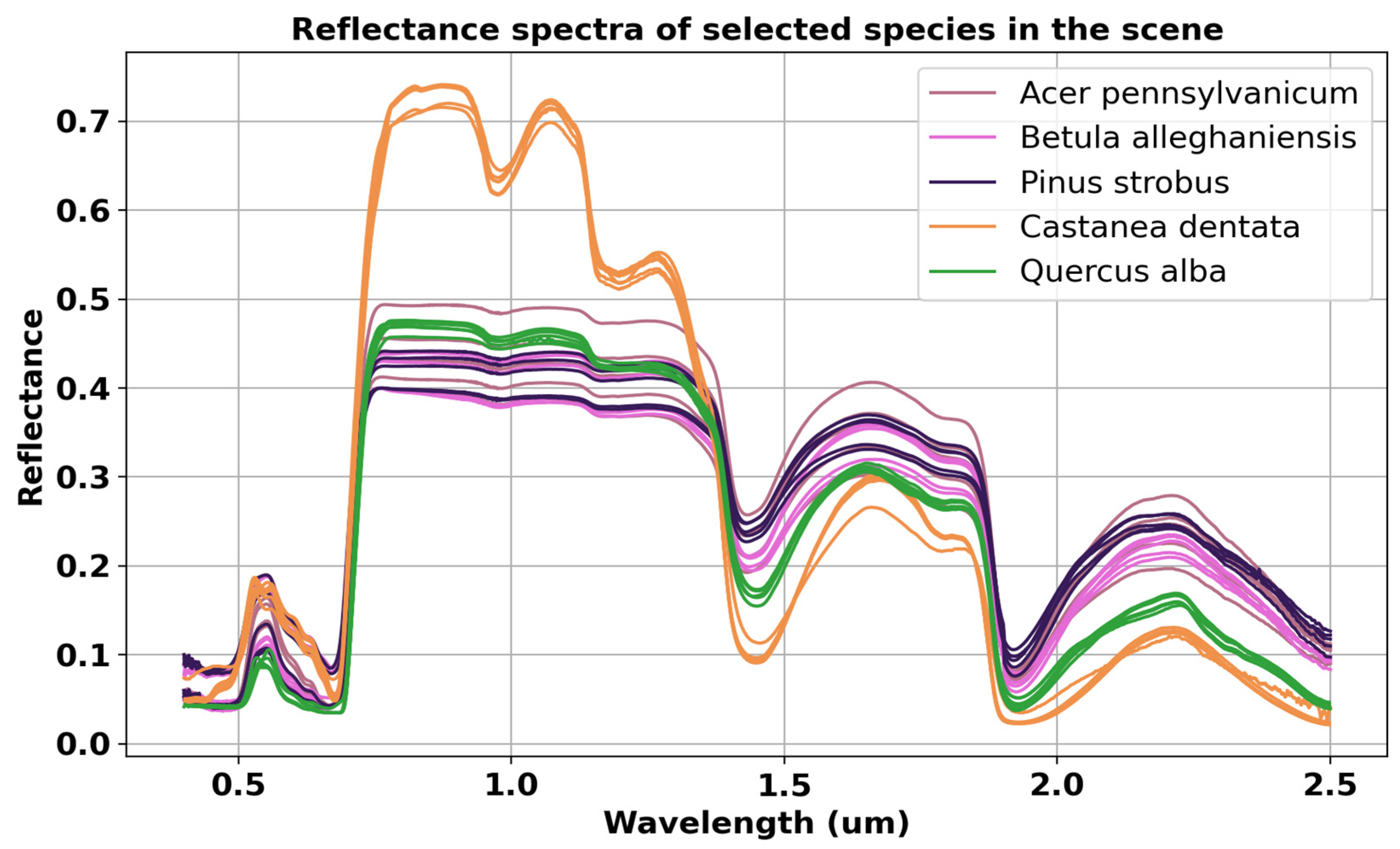
Relevant field data for this study were obtained from the online Harvard Forest Data Archive (https://harvardforest.fas.harvard.edu/, accessed on 25 January 2024). Optical characteristics, encompassing leaf reflection and transmission spectra, were derived from the ECOSIS open database (ecosis.org, accessed on 25 January 2024). Detailed taxonomy information of the plant species within the study area is shown in Table 1, where the “Class” column groups species within the same genus, simplifying classification analysis. The “Type” column, on the other hand, distinguishes between “Tree” and “Subcanopy” species, thus facilitating ecological assessments and playing a crucial role in introducing complexity to a virtual forest scene by capturing essential structural and ecological differences. We considered the tall (>6 m), dense plants with woody stems and branches as part of the canopy, and plants that had a leafy bush shape, generally low-stature, or plants with woody stems shorter than trees, as sub-canopy (note that all the plants are already subdivided into canopy and sub-canopy levels in the Harvard Forest Data Archive). Figure 2 displays reflectance spectra for a few representative species, highlighting the essential variability crucial for creating realism in virtual scene development. Along with ECOSIS database, the PROSPECT (pypi.org/project/prosail, accessed on 25 January 2024) model was used to generate the variability in individual reflectance curves for each species.

2.2. DIRSIG Simulation Development

We used DIRSIG, a physics-based first-principles radiometric modeling environment/simulation tool for the creation of synthetic imagery of the study area. DIRSIG utilizes Monte Carlo ray tracing and captures radiometrically, geometrically, and temporally accurate remote sensing images of virtual scenes [36,37,38]. We generated synthetic images of the study area using DIRSIG Version 5. Wible et al. [36] have validated the simulated scene using NEON sensor data via (i) visual inspection, (ii) spectral signatures and indices, and (iii) LiDAR data to compare the structural properties statistically. This synthetic scene uses 80 unique 3D models of vegetation to represent 28 unique species, thereby enabling the creation of multiple variants of common species, subdivided into tree and sub-canopy levels. We also added soil spectra and available bark material properties for a select set of species. Five input parameters were required for DIRSIG to generate the simulated image of the virtual Harvard Forest scene:
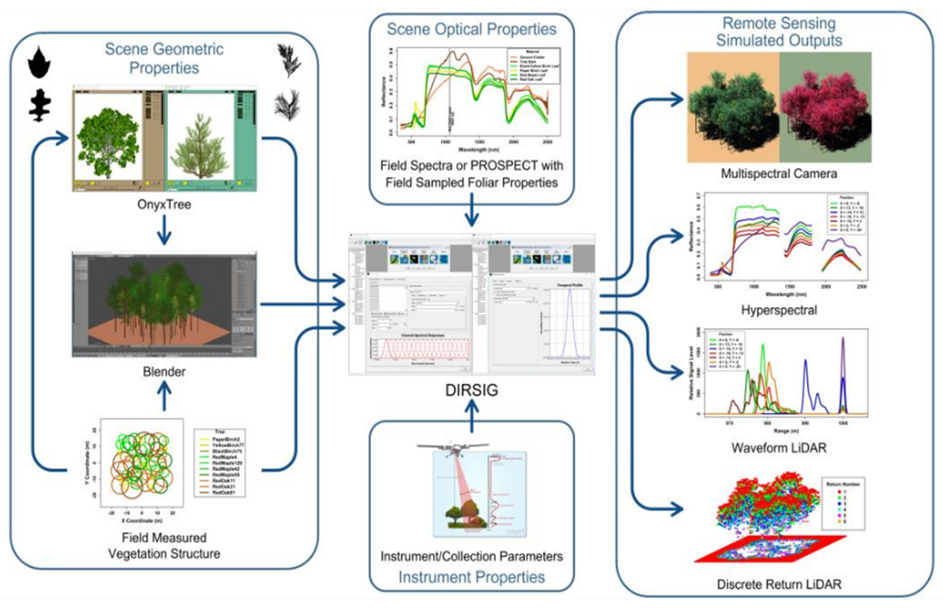
  • Scene: A DIRSIG scene is a collection of geolocated, geometric object models that include suitable optical characteristics, texture mapping, and other related attributes. We modeled 80 geometric properties of Harvard Forest vegetation (tree heights, shapes, curvatures) using the OnyxTREE software. Embedding spectral variations in the reflectance and transmittance spectra were created using PROSPECT model (pypi.org/project/prosail, accessed on 25 January 2024) by randomly adjusting leaf parameters. The geographic locations, height, and diameter at breast height (DBH) values of all plants were collected from field data and the Harvard Forest Data Archive (https://harvardforest.fas.harvard.edu/, accessed on 25 January 2024). Figure 3 illustrates the diagram of the inputs used to develop the Harvard Forest scene.
  • Atmosphere: DIRSIG uses MODTRAN4 (4v3r1) to define atmospheric conditions, including downwelling radiance, atmospheric transmission, and temperature profiles [22]. For this analysis, we used a prebuilt atmospheric model (FourCurveAtmosphere) to calculate downwelling radiance and atmospheric transmission, based on standard vertical column profiles for a midlatitude summer (MLS) environment (http://dirsig.cis.rit.edu/docs/new/four_curve_atm_plugin.html, accessed on 25 January 2024). We know that remote sensing data acquisition and analysis can be atmospherically sensitive, so for this analysis, we opted to use the same atmospheric model for all types of simulations to avoid any conflict.
  • Imaging System: The imaging system or sensor entails a methodical description of the imaging platform, encompassing the scanning technique, optical focal length, arrangement of the detector array, spectral response function, point spread function (PSF), noise properties, and other related attributes. We used AVIRIS Classic hyperspectral sensor to simulate image samples of the Harvard Forest scene. A summary of the imaging spectrometer specifications is provided in Table 2.
  • Platform Motion: The characterization of platform motion and/or position involves gathering information regarding factors such as the altitude at which it operates, its velocity, and any potential irregularities or vibrations (jitter). We used a Scene-ENU (East–North–UP) coordinate system. Since we used a fixed/static frame array sensor, platform velocity was not required.
  • Collection Details: The collection of supplementary data concerning the date and time of the task(s) impacts the sun–target–sensor geometry, along with other relevant variables. We simulated at-nadir images to avoid any sun geometry correction and took a single shot to capture the whole scene. A complete flowchart of the scene simulation is shown in Figure 4.

2.3. Preprocessing

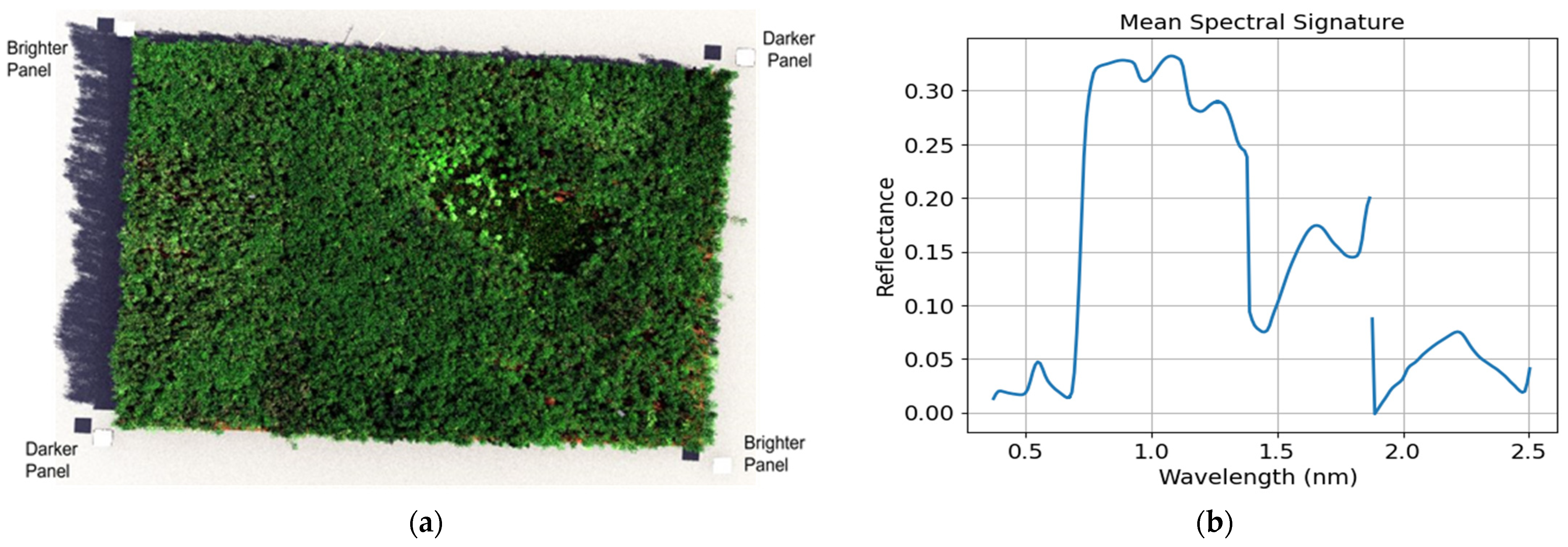
Atmospheric compensation was necessary to transform DIRSIG’s output radiance data into more tractable reflectance measurements. Previous studies have indicated that the performance of a typical spectral analysis algorithm, applied to reflectance data, is superior to the same algorithm applied to radiance data [39,40,41]. We applied the empirical line method (ELM) [41] to the simulated radiance data to generate reflectance data using the bright and dark panels (see Figure 5). The panels at opposite corners are brighter than the others. The brighter panels are 80% reflective, while the darker panels are 20% reflective. These are intended to provide two reference points for reflectance calibration across the spectral range using the ELM approach.
As previously mentioned, choosing an image that aligns with objectives of the study led to two essential inquiries: (i) to what degree does the spatial resolution of the image correspond to the research objectives of the study?; and (ii) to what extent do the spectral characteristics of an image contribute to disentangling species-specific spectral similarities or differences? Addressing these inquiries constitutes the foundational premise of our investigation into optimizing imaging spectrometers for viable tree species mapping in complex forest environments, by enhancing our understanding of the relationship between sensor parameters, resolution, and classification accuracy. In the following sections, we will describe the methodology used to compute various sensor parameters, enabling us to vary the spatial, spectral, and scale resolutions of the simulated imagery.

2.4. Computing Scene for Different Ground Sampling Distance

Ground sampling distance (GSD) is of utmost importance in order to understand the factors that determine the spatial resolution of an image. GSD refers to the distance between pixel centers on the ground, which directly influences the level of detail and spatial resolution captured by a remote sensing system.
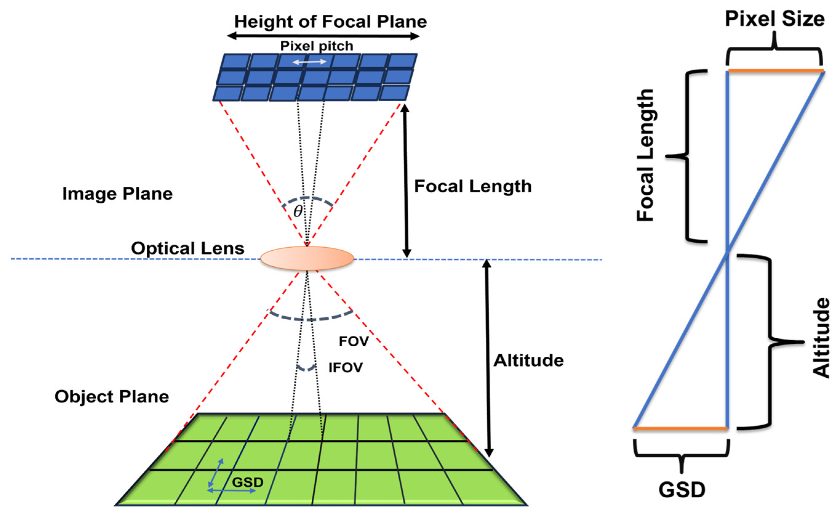
Here, we varied the GSD from 1 to 30 m by varying the flight altitude between 1 and 30 km. This range was chosen as it covers the operating range of high-resolution airborne sensors (e.g., AVIRIS, NEON, etc.) to coarser spatial resolution multispectral satellite sensors (e.g., Landsat). It is beneficial to consider the problem from a simple geometrical point-of-view (Figure 6). Considering that the spectrometer is fixed, keeping the pixel size and focal length constant, we can easily vary the GSD of the image by varying the flight altitude of the sensor (Equation (1)). It is obvious that, as the sensor approaches the ground (lower altitude), the GSD decreases, leading to a higher spatial resolution because a smaller GSD corresponds to a smaller pixel size/pitch. This means that smaller objects or features can be captured as individual pixels, leading to greater detail in the image:
P i x e l   S i z e F o c a l   L e n g t h = G S D A l t i t u d e

2.5. Computing Scenes across Different Spectral Resolutions

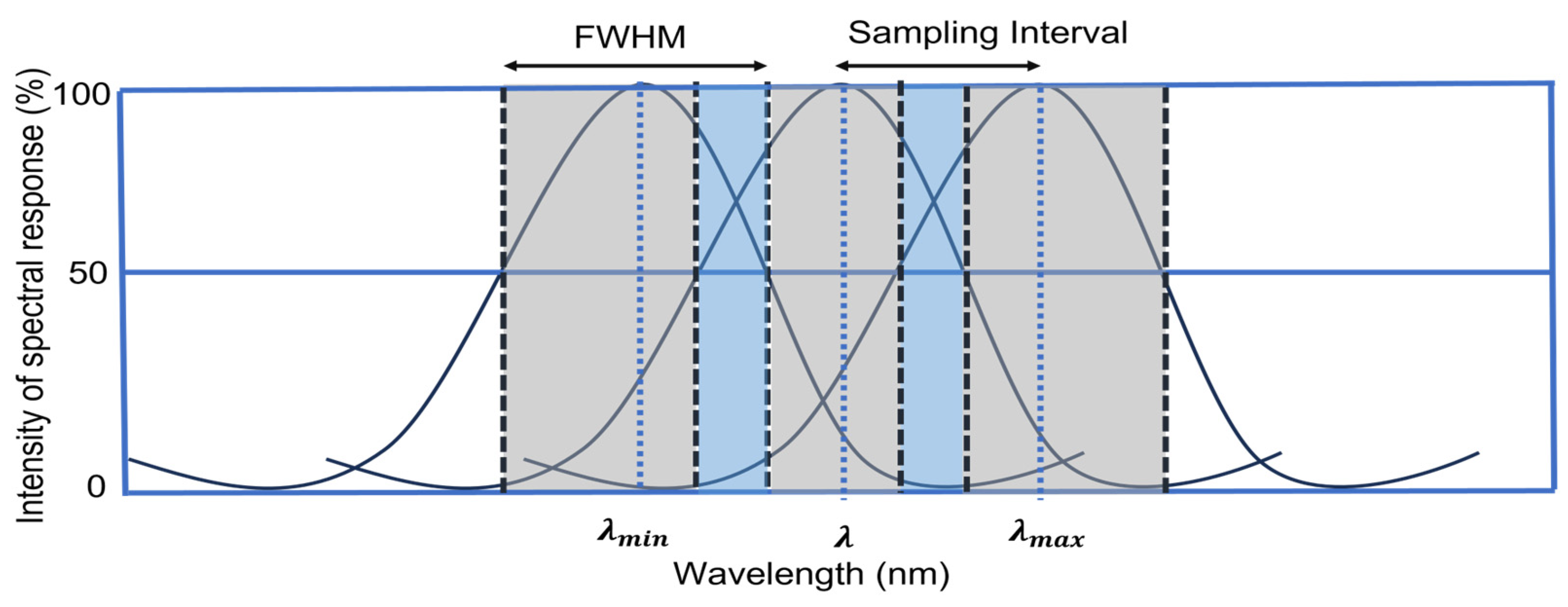
The spectral resolution is quantified in terms of the sampling rate and bandwidth of a remote sensing imaging system and used to distinguish the instrument’s ability to capture electromagnetic radiation across different wavelengths or spectral bands. The precision to differentiate between different wavelengths is usually computed using the full width at half maximum (FWHM) to define a spectral bandwidth. The FWHM is the width of a spectral line at half of its maximum intensity. High spectral resolution is characterized by a narrow bandwidth when FWHM is smaller [42].
We simulated different spectral resolutions ranging from 3 to 30 nm, with the wavelength range spanning 380–2510 nm and a total number of spectral channels/bands ranging from 714 to 69 (Table 3). We varied the spectral resolution in two primary ways, by adjusting the FWHM and by altering the spectral sampling, as shown in Figure 7. Narrower FWHM values and increasing the spectral sampling resulted in a higher spectral resolution, as they allowed for a finer discrimination of subtle variations in the spectral signature of different materials. In addition, we simulated images using a multispectral sensor (MS) with eight bands in the silicon range (400–1000 nm), carefully selected to avoid spectral overlap and maintain distinct spectral information. These wider FWHM values for the MS resulted in obvious decreased spectral resolution, but it allowed for broader wavelength coverage, thereby capturing more information across a wider range.

2.6. Computing Scenes at Different Scale Resolutions

It is common practice in remote sensing studies to discuss the spatial and spectral resolution of systems, while not much attention is paid to the scale resolution of the camera/imaging equipment used in the sensor. It is an important characteristic that defines the pixel array dimension of a sensor. We determined sensor scale resolutions by modifying the pixel pitch and the total number of pixels in the sensor array, i.e., the focal plane dimension.
We can see from the geometric illustration in Figure 6 that the height of the focal plane, which determines the scale resolution of the imaging sensor, is the multiplication of the total number of pixels and the corresponding pixel size/pitch (Equation (2)). The relationship of the total number of pixels to the pixel size is also related to the focal length:
tan θ 2 = H e i g h t   o f   t h e   F o c a l   p l a n e 2 × F o c a l   L e n g t h
If we want to keep the focal length constant so that the field of view, θ , of the sensor does not change, and if we increase the total number of pixels by, say, a factor of two, then we must decrease the pixel size by dividing that value by two. In other words, if we define more pixels in the array, the pixel size needs to be proportionally smaller so that the overall size of the detector does not change with respect to the focal length.
We explored the impact of the sensor scale resolution on species classification by keeping all other parameters constant and varying the total pixel count and pixel size of the imaging sensor, thereby isolating the effect of scale resolution. For instance, in Figure 8, we show three examples of scale resolution: low, medium, and high pixel density images. We assume that these sensors’ heights of the focal plane are constant and changes in scale resolution necessitate considering the inverse relationship between the total number of pixels and pixel size. The leftmost sensor has a low pixel density, so in order to maintain a constant sensor size, a larger pixel pitch or size is required—this outcome would be a lower scale resolution sensor with larger signal-to-noise ratio (SNR). Conversely, the rightmost sensor has a smaller pixel size with a high pixel density image, and it can be equated to a higher-scale resolution sensor with a smaller SNR. Considering the impact of different sensor scale resolutions on the SNR is crucial in sensor design, as it ultimately influences both spectral and spatial resolutions. As we focus to demonstrate the utility of simulation tools in designing application-specific sensors in this analysis, we acknowledge that this study did not involve a detailed analysis of SNR, or the determination of the minimum SNR required to maintain specific spectral or spatial resolutions.
However, in our study, we investigated three scale resolution levels (0.5X, 1X, and 2X (Table 4)) and their impact on species classification in the simulated Harvard Forest scene. The AVIRIS Classic sensor employed in our simulation had a pixel array dimension of 667 × 552, with each pixel measuring 200 microns, denoted as the 1X resolution sensor. We subsequently halved the pixel array to achieve the 0.5X resolution and doubled it for the 2X resolution:
H e i g h t   o f   S e n s o r   F o c a l   P l a n e = T o t a l   N u m b e r   o f   P i x e l s   × P i x e l   S i z e
Next, we will discuss our choice of classification algorithm, applied across the various sensor configurations, for the purpose of species classification (our proxy application). It is worth highlighting that our intent was not to evaluate the efficacy of different classifiers, but rather to assess the outcome of different sensor configurations.

2.7. Deep Learning Algorithm

A convolutional neural network (CNN) is a class of deep neural networks, most commonly used for image recognition and processing, due to its ability to recognize patterns in images. The current leading CNN architectures in the field are VGG16/19, GoogLeNet, DenseNet, Inception, and ResNet [34], all of which are commonly used for general image classification tasks that involve classifying a large number of classes (typically more than 1000). However, for classification problems with a limited number of classes (24 classes in our specific case), these architectures tend to be excessively complex and computationally intensive. Moreover, previous studies have demonstrated that these larger CNN models do not outperform the smaller models in classification tasks in forestry applications [44,45]. A smaller 1DCNN architecture (Figure 9) was therefore developed to address the classification of the simulated Harvard Forest scene. We discovered, after evaluating various architectures, that a sequential model design featuring two consecutive convolution/pooling layers yielded the best performance for our simulated dataset. The complete model architecture is shown in Figure 9.
This design was optimized to classify our simulated images into 22 distinct genus-level species classes and bark, soil classes (total 24) (Table 1, column name: class). All convolutional layers, along with the fully connected layer, employed the rectified linear unit (ReLU) activation function [46]. For the final classification layer, we utilized the SoftMax activation function [47]. We incorporated two dropout layers with a dropout rate of 0.4 into the model in order to enhance the performance and prevent overfitting. Dropout regularization simplifies the network and improves the robustness of the machine learning model [48]. In comparison to larger architectures, our model is significantly smaller and has lower computational requirements, with only 82,429 trainable parameters. This is in stark contrast with some of the smallest of the larger architectures that contain over 25 million trainable parameters. Categorical cross-entropy loss and Adam optimization (a gradient descent method) [49] were used for all model training/validation runs in this study. The models were trained with a batch size of 256, for a total of 100 epochs. However, extending the training beyond this point did not yield any notable improvement in the validation accuracy. The implementation and training of the model were carried out using TensorFlow, a large-scale machine learning library, along with the Keras deep learning API [47].
We conducted a comparative analysis with two other classification approaches to assess the efficacy of the 1DCNN architecture employed in this study, namely a traditional machine learning classifier (support vector machine; SVM) [50] and a state-of-the-art deep learning architecture, called HybridSN [51]. SVM is a supervised algorithm, used for solving complex classification problems involving multispectral and hyperspectral data, where distinguishing target features based on spectral variations can be challenging. We used the typical feature selection algorithm, i.e., PCA (principal component analysis) [52], to curtail the redundancy of information in our simulated hyperspectral data, before applying the SVM. HybridSN, on the other hand, is a deep learning architecture that combines a spectral–spatial 3D-CNN, followed by spatial 2D-CNN layers. It has been demonstrated to achieve exceptional classification accuracy and exhibit robustness across diverse datasets [51].

2.8. CNN Training and Testing

The splitting of a dataset into a training and testing set is a model validation procedure that enables researchers to simulate how a model would perform on new/unseen data. We used Scikit-learn to split the dataset into 70% training data and 30% testing data. Table 5 presents the number of samples available as training and testing datasets for imagery of different resolutions by varying their ground sample distance (GSD). It can be seen that the number of observations started decreasing with coarser resolution, i.e., when we increased the GSD value.

2.9. Accuracy Metrics

Deep learning models are evaluated based on their performance and accuracy in classification tasks. Such assessments involve analyzing a confusion matrix generated from the test dataset to determine various performance parameters. The confusion matrix consists of diagonal elements representing correct classifications and non-diagonal elements indicating misclassifications [53]. The typical elements of the confusion matrix are defined as follows:
  • True Positive (TP): Accurately labeled positive samples by the classifier.
  • True Negative (TN): Accurately labeled negative samples by the classifier.
  • False Positive (FP): Incorrectly labeled negative samples as positive.
  • False Negative (FN): Incorrectly labeled positive samples as negative.
We considered macro recall, macro precision, macro F1 score, and mean accuracy to evaluate model performance. Sensitivity/recall, often referred to as the true positive rate, measures the model’s ability to correctly detect positive class samples. Precision assesses the model’s accuracy in assigning positive events to the positive class. Macro recall calculates the average effectiveness of the classifier in identifying class labels, while macro precision evaluates the average agreement between the data class labels and those assigned by the classifier. The F1 score represents the harmonic mean of recall and precision. Accuracy, on the other hand, quantifies the ratio of correct predictions to all predictions made. Furthermore, Cohen’s kappa coefficient measures the level of agreement between the predicted and actual classifications [54]:
S e n s i t i v i t y / R e c a l l = T P T P + F N
M a c r o   R e c a l l = n = 1 C R e c a l l C = N o   o f   C l a s s e s
P r e c i s i o n = T P T P + F P
M a c r o   P r e c i s i o n = n = 1 C P r e c i s i o n C = N o   o f   C l a s s e s
F 1   s c o r e = 2 × P r e c i s i o n × R e c a l l P r e c i s i o n + R e c a l l
W e i g h t e d   A v e r a g e   R e c a l l = n = 1 C R e c a l l × N n = 1 C N = R e s p e c t i v e   n o   o f   s a m p l e s   i n   e a c h   c l a s s
W e i g h t e d   A v e r a g e   P r e c i s i o n = n = 1 C P r e c i s i o n × N n = 1 C N = R e s p e c t i v e   n o   o f   s a m p l e s   i n   e a c h   c l a s s
C o h e n   K a p p a   C o e f f i c i e n t = 2 × ( T P × T N F N × F P ) T P + F P × F P + T N + ( T P + F N ) × ( F N + T N )

3. Results and Discussion

3.1. Simulated Scenes for Different GSD

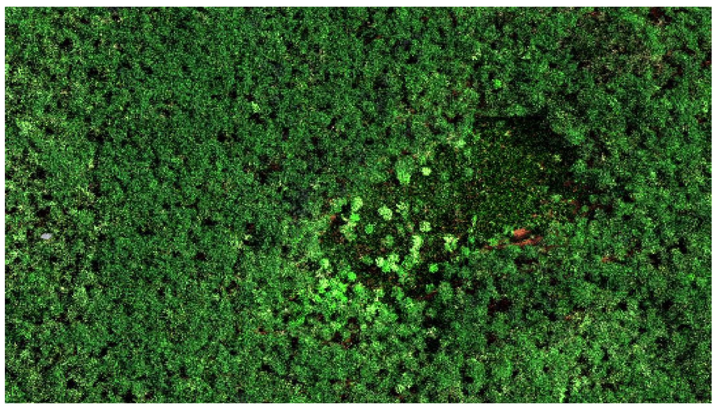
The DIRSIG scene generation process demonstrated its capability to intricately arrange individual plant models within a given scene and calculate the reflectance from any desired perspective. Figure 10 presents the simulated scene, captured at nadir, based on a true-color AVIRIS sensor rendering. The rendered image exhibits a notable level of realism, showcasing visible variations in apparent leaf reflectance. These variations stem from the diverse species present, the orientation of individual leaves, and the interplay of shadows within and between plant canopies. Although not immediately discernible in the nadir images presented in Figure 10, certain individual plants may be situated in the understory or sub-canopy. Consequently, not all species within the scene are visible from a single viewing angle.
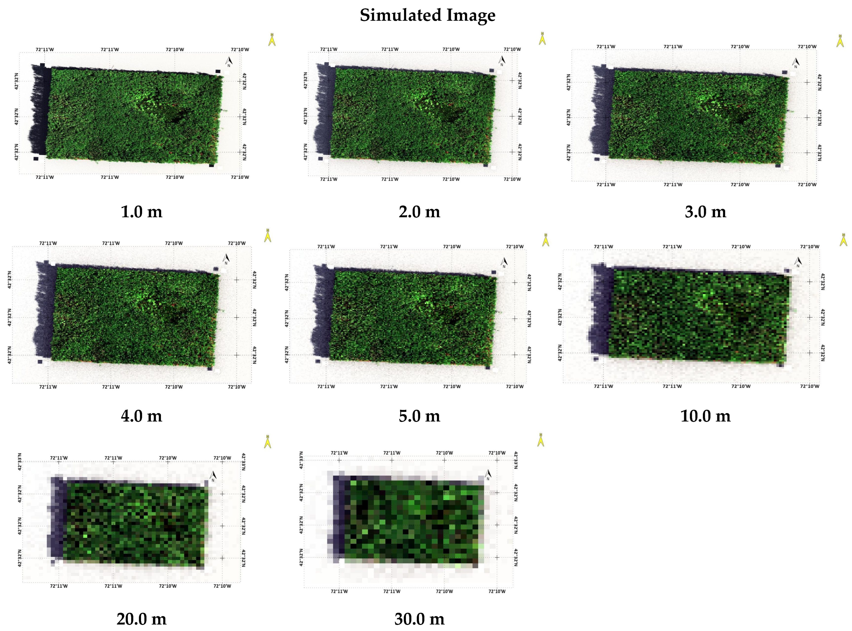
We generated eight synthetic scene layouts to evaluate the impact of different GSDs. These scenes were simulated by varying the altitude from 1 to 30 km and produced 1 m, 2 m, 3 m, 4 m, 5 m, 10 m, 20 m, and 30 m spatial resolution imagery (Figure 11). This range of resolutions covers the operating range of airborne to spaceborne imaging spectrometers. These simulated images will be used later to test the performance of classifiers in the complex forest scene imagery at different spatial resolutions. All renderings for this particular experiment were 667 × 512 pixels with 224 spectral bands.

3.2. Ground Truth Map for Different GSD Values

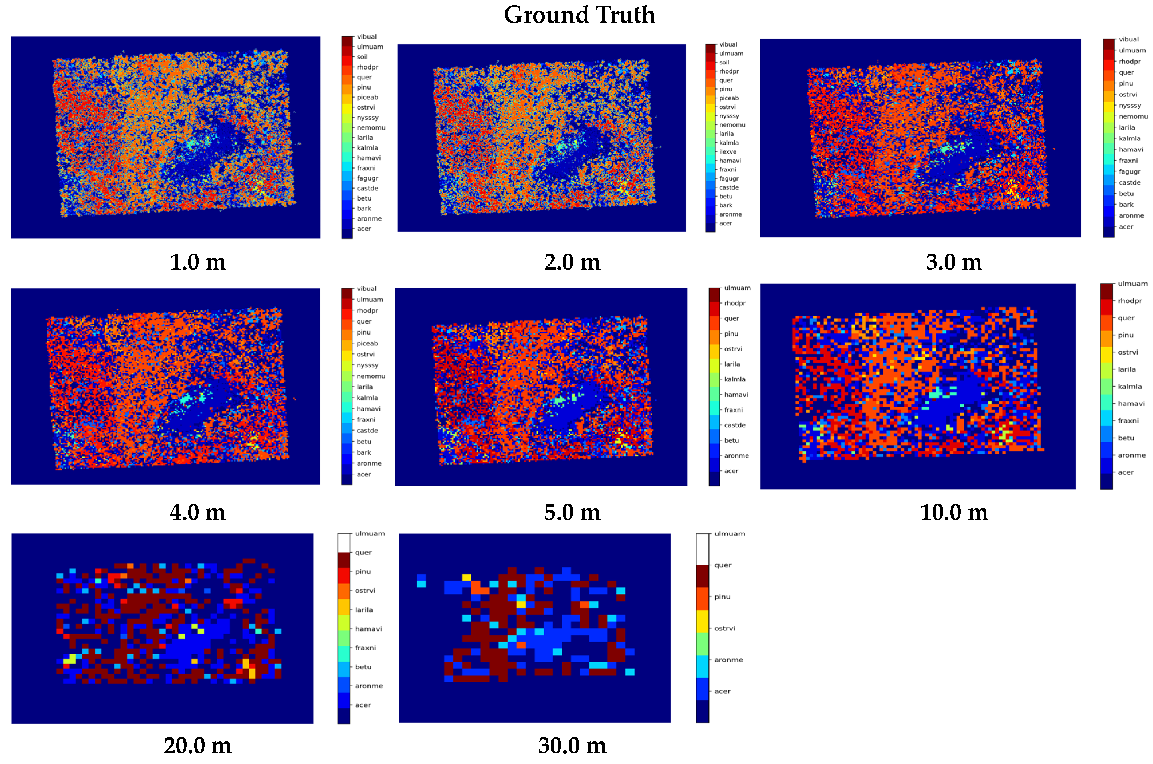
The DIRSIG model includes a corresponding ground truth map that extracts per-pixel information in terms of materials present within each pixel. These maps are created by tracing primary rays from the camera’s perspective upward, until they intersect with the scene, effectively assigning each species to its corresponding image pixel in our case. The ground truth maps, depicted in Figure 12, have the same dimensions as the simulated images. They served as essential references for validating the accuracy of species classifications derived from the canopy-level spectral reflectance, thus enabling the study of how different sets of sensor parameters affect species classification (https://dirsig.cis.rit.edu/docs/new/truth.html#_truth_image_file, accessed on 25 January 2024).

3.3. Classification Performance for Imagery of Different GSDs

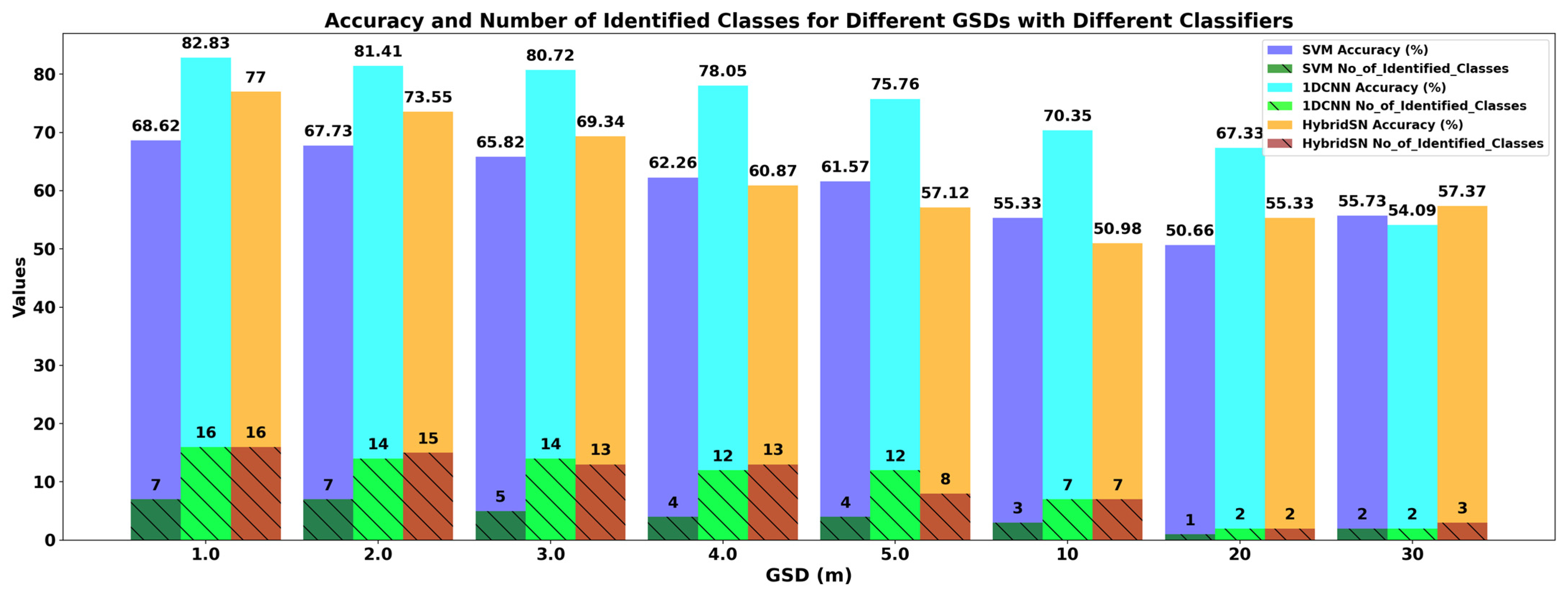
The classification metrics, including the highest overall accuracy (OA), kappa coefficient, F1 score, precision, and recall of the 1DCNN model, HybridSN, and PCA-SVM for different GSD values are shown in Table 6, Table 7 and Table 8, respectively. Among all the sample sets (1–30 m), the 1DCNN exhibited the highest OA, kappa coefficient, F1 score, macro average precision, weighted average precision, macro average recall, and weighted average recall values, i.e., values higher than HybridSN and PCA-SVM except a 30 m GSD. In the best-case scenario, or a GSD = 1 m, the 1DCNN boasted an OA = 82.83% and kappa coefficient = 77.51%, and with the HybridSN model, we have achieved an OA = 76.94% and a kappa coefficient = 69.81%, whereas the traditional SVM classifier returned an OA = 68.62% and a kappa coefficient = 57.33%. Across the worst-case scenarios, i.e., at 30 m GSD, the 1DCNN model resulted in an OA = 54.09% and a kappa coefficient = 18.70%. The HybridSN model, in turn, attained an OA = 57.37% and kappa coefficient = 30.37% and SVM showed an OA = 55.73%, accompanied by a kappa coefficient = 15.01%. Figure 13 presents the bar chart showing the highest OA vs. the total number of identified classes for different classifiers. At 1 m GSD, when the sensor captures the highest spatial resolution image, the traditional SVM classifier identified only seven individual classes, whereas the 1DCNN and HybridSN identified sixteen classes. Overall, it is evident that the deep learning classifiers performed better than the traditional approach (SVM). However, the HybridSN model required more computational time than the 1DCNN model. We concluded that 1DCNN outperformed the state-of-the-art HybrisSN algorithm, based on the results and considering the computational expense.
It is rather obvious that higher GSD values lead to a decrease in image resolution, consequently impacting the performance of the classifiers. Thus, it is observed that the classifiers performed better at a GSD = 1 m, particularly the 1DCNN and HybridSN models, which successfully identified sixteen classes. Conversely, at 30 m spatial resolution, only two or three dominant genus-level species classes can be discerned by the CNN. Table 5 further demonstrates a significant reduction in the number of training samples as the resolution coarsens. The model’s performance improves with a larger number of training samples, and when the imagery resolution is low, only a few training samples per species are available, thus influencing the classification accuracy.
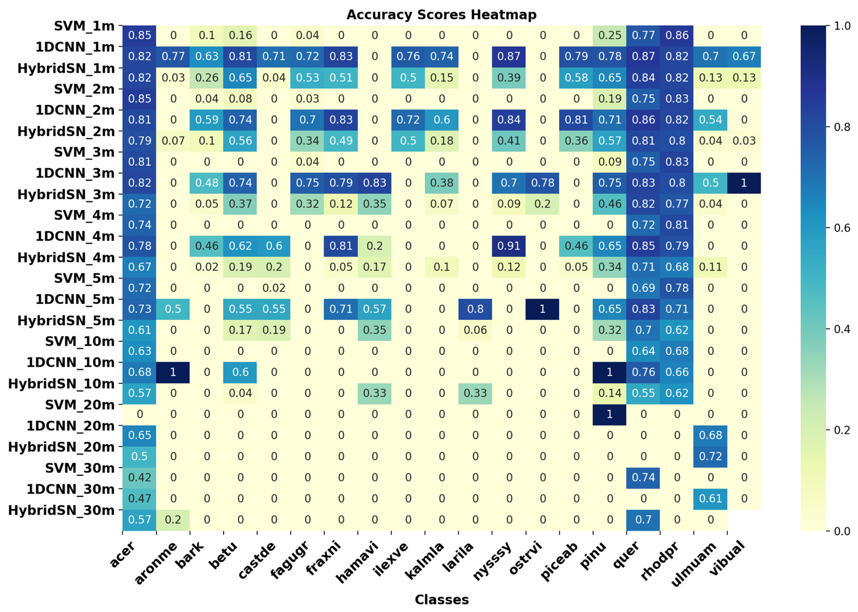
Figure 14 presents the heatmap of recall/accuracy per class for different GSD images. The acer, pinu, and quer are different dominant genus-level classes in the Harvard Forest plot. We can see that at 1 m GSD, the highest accuracies for acer, pinu, and quer were 85%, 78%, and 87%, respectively. It was also found that a 1 m spatial resolution (1 m GSD) imagery generally provided better performance than other samples, but sometimes a better accuracy was achieved at coarser resolutions, e.g., pinu at 100% accuracy for GSD = 10 m. However, higher spatial resolution comes at the expense of a reduced coverage area per image and generates a larger amount of data per unit area. As a result, the computational costs of simulating, processing, and applying the classification algorithm increased when we used the 1 m GSD image. Practically, to obtain a GSD = 1 m image over the Harvard Forest scene (500 × 700 m), we needed to fly at 1000 m altitude and a single shot at this low altitude did not allow us to capture the whole scene. We therefore had to apply mosaicking algorithms, which increased the required pre-processing steps and made the image large enough to introduce a substantial increase in computational time to run algorithms. This is also applicable to real-world image collection at higher spatial resolutions. However, if we look closely at the heatmap/performance matrices of 1 m and 2 m GSD images, we see a small change in the overall performance of the classifiers. At 2 m GSD, a single shot was enough to capture the whole scene and it took less time to run the deep learning algorithms.
Unfortunately, in remote sensing, there is no “one size fits all” choice when it comes to spatial resolution. Simulating different spatial resolution/GSD imagery allows for flexibility in choosing the appropriate level of detail for a specific task. Accurate feature extraction and object identification often necessitate high spatial resolution imagery. Our results demonstrated that spatial resolutions ranging from 1 to 3 m yielded improved accuracy in classifying genus-level tree classes within complex forest scenes, such as Harvard Forest. For applications focused on capturing dominant genus classes like acer, pinu, or quer in the simulated scene, airborne sensors operating at 10–30 m GSD can be suitable. We also know that large-area mapping or change detection tasks may not require (or be amenable to) high spatial resolution imagery, making lower spatial resolution imagery sufficient.
The findings on the classification performance for imagery of different ground sampling distances (GSDs) have practical implications for guiding the optimization of remote sensing mission resources. This research contributes by enhancing our understanding of the nuanced relationship between spatial resolution and classification accuracy in complex forest environments, thus informing the design of future imaging spectrometers. These insights hold broader significance for policy and practice in remote sensing agencies, influencing decision making in resource allocation for environmental monitoring. Additionally, the study lays the groundwork for future research directions, encouraging further exploration into the optimization of system specifications for accurate tree species mapping.
We acknowledge a crucial yet unexplored factor within our study, in addition to our findings on the positive correlation between higher spatial resolutions and classification accuracy, namely the impact of object size on classification performance. The “optimal” resolution may vary if object size, on average, exhibits larger (e.g., larger crowns) or smaller sizes. For instance, in agriculture, the accurate discrimination of “weed” species from crops necessitates a resolution significantly finer than 1 m, while coarser resolutions might suffice for broader land-use classification scenarios. Explicitly accounting for object size and its ramifications on sensor specifications is essential for maximizing the generalizability and impact of our findings, and thus has to inform the selection of appropriate resolutions for diverse contexts and applications.

3.4. Classification Performance for Imagery of Different Spectral Resolutions

The objective of this experiment is not to establish the superiority of one classifier over another, but rather to evaluate the appropriate specifications of an imaging sensor that aligns with a specific remote sensing application. Based on the results of the earlier experiment, which indicated the superior performance of 1DCNN compared to HybridSN and SVM-PCA, we have chosen to constrain the study to the 1DCNN for the subsequent experiments. We have designed three different setups, varying the spectral resolution from 3 to 30 nm, and included a multispectral setup for three different GSDs, namely 1 m, 5 m, and 10 m. The performance accuracy of 1DCNN was calculated for all samples within these setups.

3.4.1. Different Spectral Resolutions at 1 m GSD

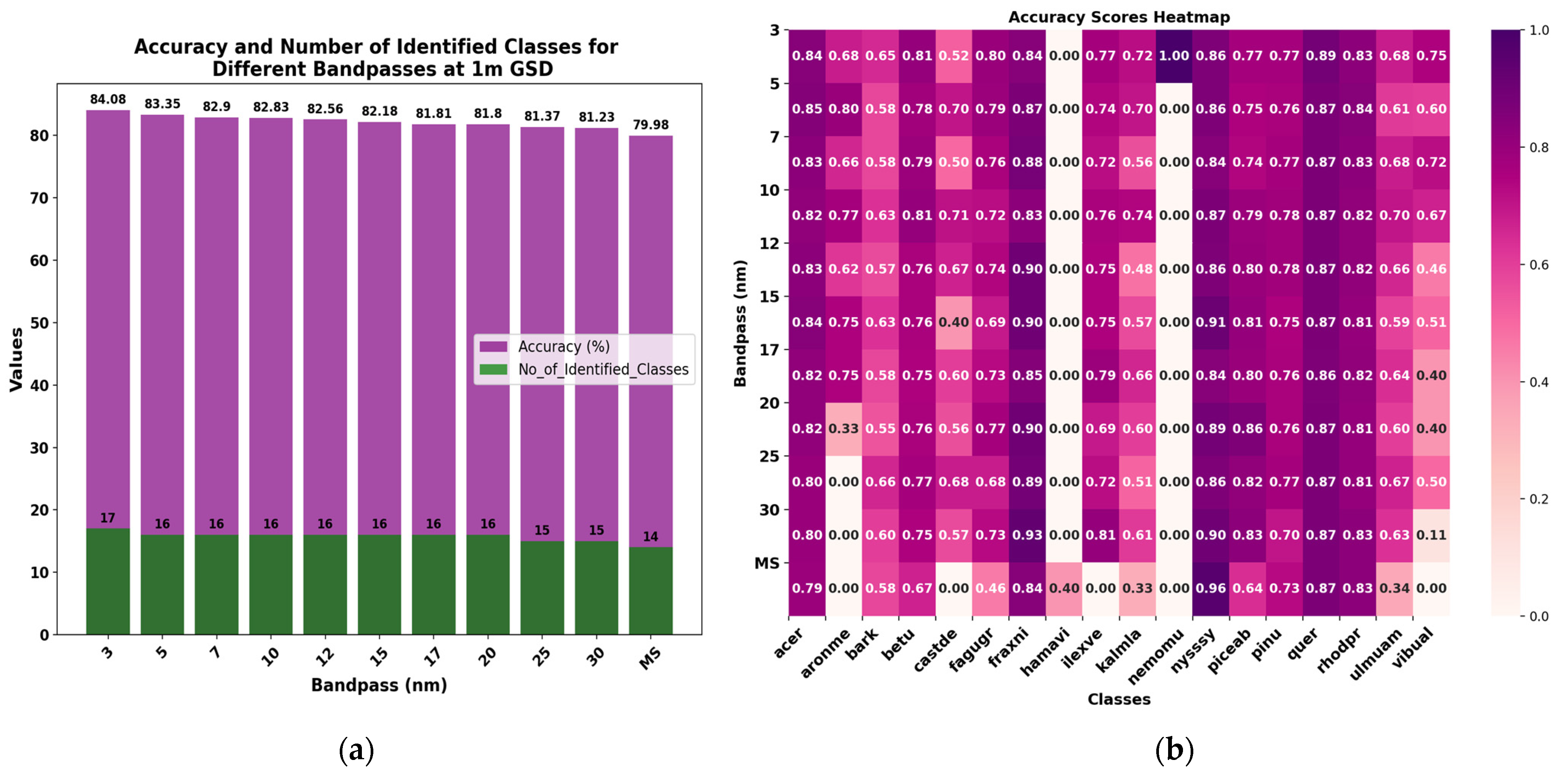
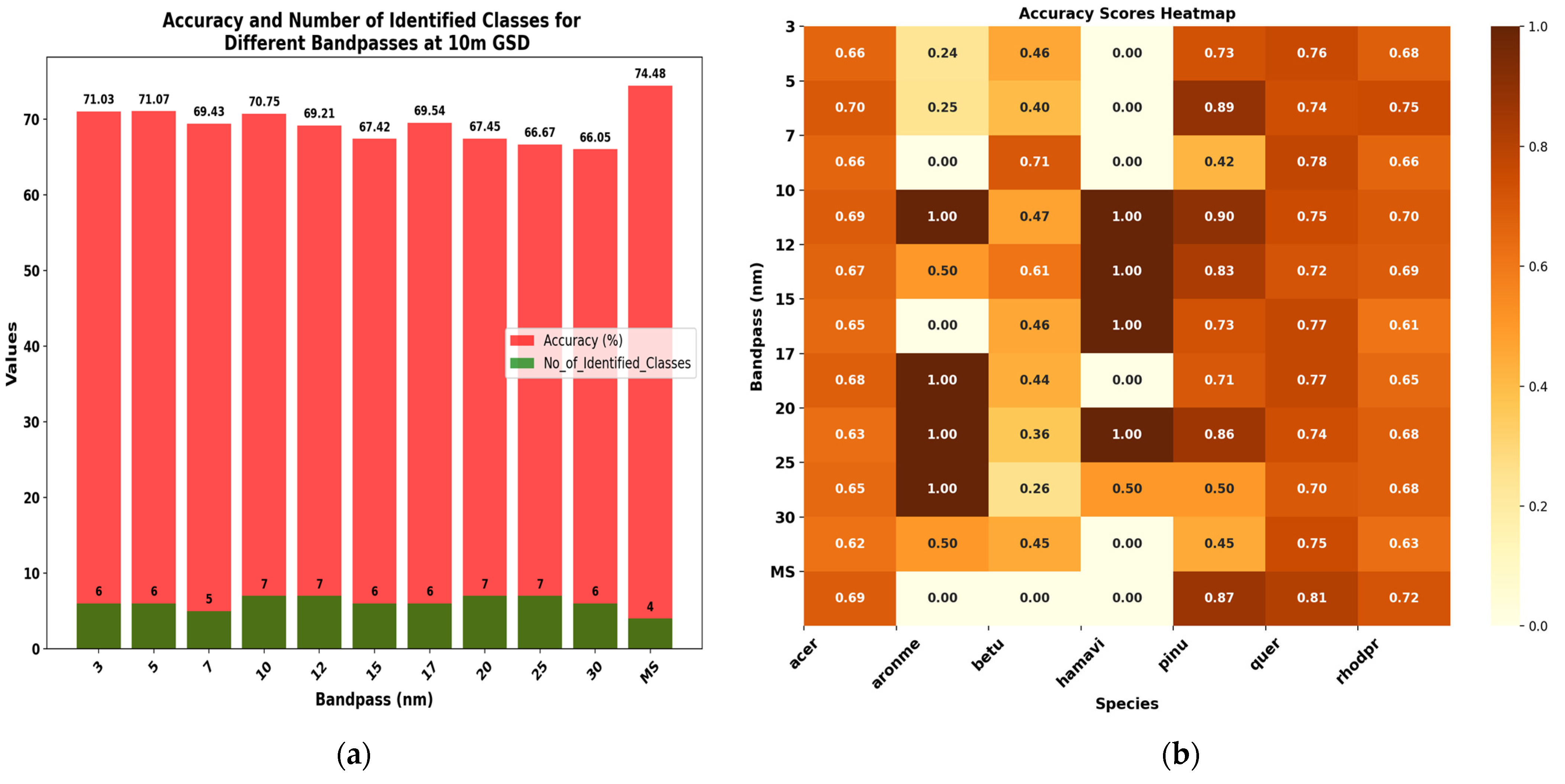
Table 9 presents the overall accuracy, kappa coefficient, F1 score, precision, and recall of the 1DCNN model for different spectral resolutions. The highest OA ranged from about 80–84%, while the kappa coefficient ranged from 73 to 79%. Figure 15a displays a bar chart depicting the range of identified classes, which varied from 14 to 17. Furthermore, Figure 15b shows a heatmap illustrating the per-class accuracy of genus-level species classes across different spectral resolutions.
Among all the sample sets, the 3 nm spectral bandpass at 1 m GSD and a flight altitude of 1000 m boasted the best performance matrices. We obtained 714 bands at 3 nm spectral resolution; moreover, applying the classification algorithm to this image yielded an accuracy of 84.08%, and the classifier could identify 17 different species. Conversely, at a spectral resolution of 30 nm, we only had 69 bands and achieved an accuracy of 81.23% with 15 species. We observed that at 3 nm, we could identify 17 classes, while at spectral resolutions ranging from 5 to 20 nm, we could identify 16 classes when comparing the overall performance matrices for these different spectral resolutions. At 25–30 nm, the number of identifiable classes decreased to 15, with slight variations in their performance accuracy. Surprisingly, when we reduced the spectral resolution to eight non-overlapping bands (referred to as multispectral or MS), the 1DCNN algorithm could still identify 14 genus-level species classes with an impressive classification accuracy of up to 80%.
The question arises whether it is worthwhile to collect 714 bands to achieve only a 1–2% improvement in accuracy. It is important to consider that a higher spectral resolution can reduce the signal-to-noise ratio (SNR) of the sensor output. With a larger number of spectral bands, there is an increased likelihood of capturing unwanted atmospheric interference, which can adversely affect the accuracy and reliability of the data analysis. Moreover, limitations related to sensor design (e.g., silicon range (400–1000 nm) sensors are much cheaper), data transmission, and storage capacity should also be taken into account [55]. From an algorithmic perspective, deep learning algorithms tend to perform better with a larger number of training samples. However, it is evident that redundant spectral information did not significantly enhance the accuracy, but instead increased the computational time. It therefore may be a viable option to use a sensor with a high spatial resolution, such as 1 m GSD, combined with a multi-spectral resolution or a lower spectral resolution, which can provide an accuracy of approximately 80% when using the CNN. This is especially important when considering the tradeoff between spectral and spatial resolutions (a sensor with a high spatial resolution usually has a lower spectral resolution, and vice versa [56]).

3.4.2. Evaluating Different Spectral Resolutions at GSD = 5 m and GSD = 10 m

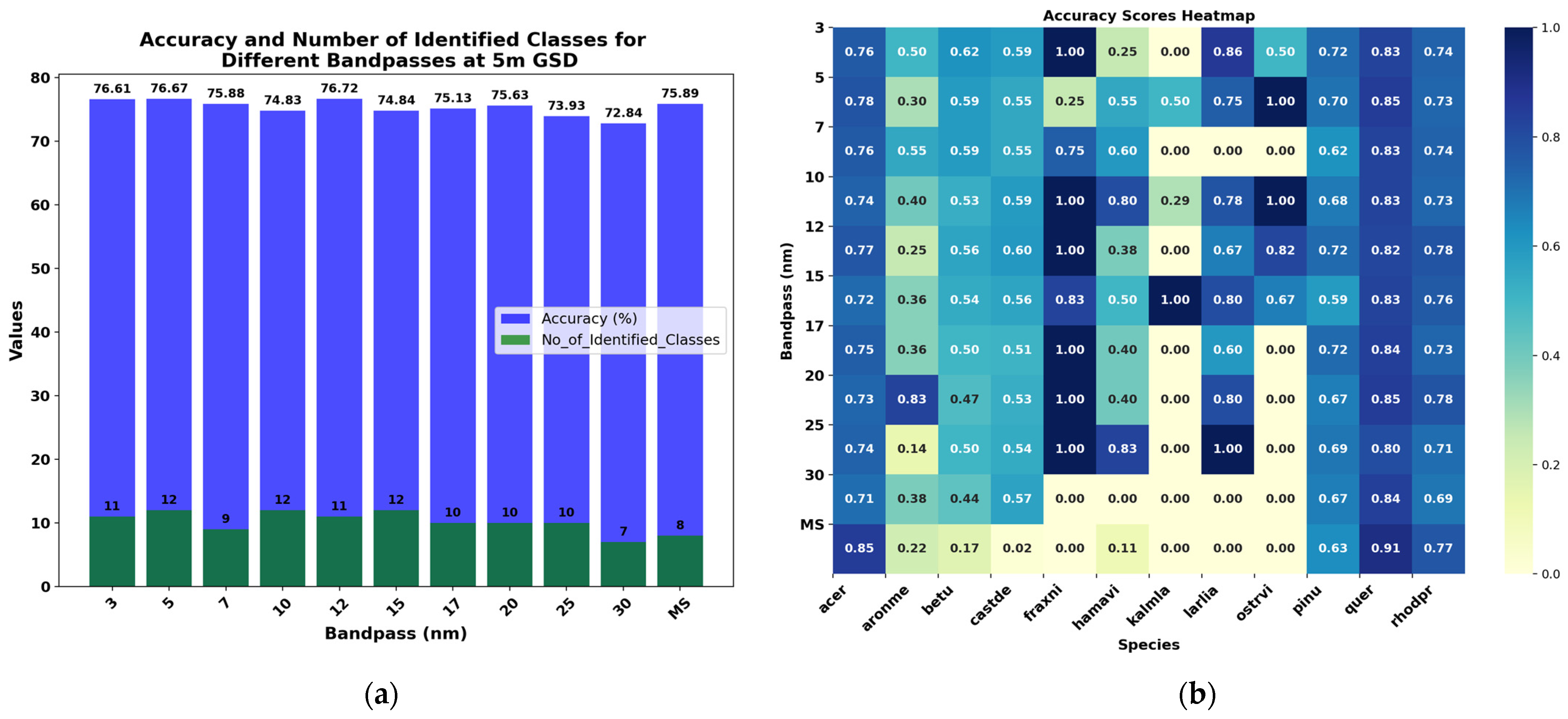
We examined the impact of varying the spectral resolution at 5 m and 10 m GSDs, in order to assess the consistency of our findings reported in Section 3.4.1. Table 10 and Table 11 present the overall accuracy, kappa coefficient, F1 score, precision, and recall of the 1DCNN model for different spectral resolutions at 5 m and 10 m GSDs, respectively. At a flight altitude of 5000 m with GSD = 5 m, a change in the spectral resolution from 3 to 30 nm as well as using the multispectral (MS) sensor resulted in overall accuracies ranging from approximately 72–76%, with kappa coefficients of 62–76%. It should be noted that the dataset is imbalanced, which explains the lower macro average precision and recall values compared to the weighted average values. Furthermore, we can see from Figure 16a that the 1DCNN identified 7–12 individual genus-level species classes across different spectral resolutions. Figure 16b illustrates the heatmap of per-class accuracy, highlighting that the MS resolution achieved the highest individual accuracies for acer (85%), quer (91%), and rhodpr (77%), contributing to the overall accuracy of 75.89%. Overall, the 3 nm and 5 nm spectral resolutions at GSD = 5 m yielded the highest overall accuracy of 77% and a kappa coefficient of 68%, while the 30 nm spectral resolution resulted in the lowest overall accuracy of 73% and a kappa coefficient of 62%.
The classification results (Table 11) showed an overall accuracy ranging from approximately 66 to 74% at GSD = 10 m. The kappa coefficient, which measures the agreement between predicted and observed classifications, ranged between 52 and 63%. Between four and seven individual genus classes were identified from the imagery, as demonstrated in Figure 17a. It can be observed from Figure 17b that the highest accuracy was achieved for specific genus classes, such as acer (70% at 5 nm), aronme (100% at 10 nm, 17 nm, 20 nm, 25 nm), betu (71% at 7 nm), hamavi (100% at 10 nm, 12 nm, 15 nm, 20 nm), pinu (90% at 10 nm), quer (81% at multispectral), and rhodpr (75% at 5 nm). However, it can be seen that for the multispectral resolution case, the CNN achieved the highest overall accuracy of 74%, but it could only identify four individual genus classes, which primarily represented the dominant genus classes within the scene. Furthermore, based on the total number of identified species, per-class accuracy, and other performance metrics, it was concluded that spectral resolutions ranging from 3 to 10 nm offer the best overall accuracy (OA) of approximately 70%, with a kappa coefficient of around 60%. Spectral resolutions between 20 and 30 nm, on the other hand, resulted in the lowest OA of approximately 66% and a kappa coefficient of around 52%. It is worth noting that at a flight altitude of 10,000 m (GSD = 10 m), the classification mainly identifies the dominant genus classes regardless of the spectral resolution used.
Our findings indicate that spatial resolution has a greater impact on genus-level species classification when compared to spectral resolution, which is particularly evident in the results of GSD = 1 m at different spectral resolutions. It is important to note that this study is based on synthetic data. Although we incorporated field spectral data and the ECOSIS database to simulate species spectra in the Harvard Forest scene, we did assume that the use of the PROSPECT model to generate multiple instances of the same species introduced at least some uncertainty in the overall spectral sensitivity analysis. Nevertheless, our results show that a multispectral resolution is sufficient for capturing the dominant genus classes up to GSD = 10 m. It should, however, be acknowledged that certain absorption features in the vegetation species exhibit unique spectral behavior [57], which cannot be fully captured by a multispectral sensor. For a more accurate identification of vegetation species with similar spectral properties, the use of an imaging spectrometer may be necessary, despite the challenges associated with the increased dimensionality of the data. However, our analysis indicates that when we have higher spatial resolution, we can compromise on spectral resolution to achieve acceptable classification results, and vice versa. It is crucial to consider this tradeoff when designing imaging sensors, i.e., to ensure that they are optimized to meet the specific requirements of the remote sensing task at hand. However, this study enhances our understanding of the nuanced spectral resolution requirements for accurate tree species mapping in complex forest scenes. From a practical standpoint, this insight can guide the development and utilization of sensors in real-world applications such as forestry, ecology studies, and environmental monitoring, and improve the efficacy of application-specific remote sensing practices.

3.5. Classification Performance for Different Sensor-Scale-Resolution Imagery

Next, we examined the impact of varying the scale resolution on classification performance. We altered the number of pixels and pixel size, while keeping other parameters constant, thus keeping the sensor dimension stable. We conducted six setups with varying scale resolutions: 0.5X to 2X for imagery captured at (i) GSD = 5 m and 10 nm spectral resolution, (ii) GSD = 5 m and 20 nm spectral resolution, (iii) GSD = 10 m and 10 nm spectral resolution, (iv) GSD = 10 m and 20 nm spectral resolution, (v) GSD = 5 m and multispectral resolution, and (vi) GSD = 10 m and multispectral resolution. We evaluated the performance accuracy of the 1DCNN model for each different sample. The primary objective of this experiment was to investigate how classification performance can be enhanced in lower-spatial-resolution sensor setups. Our previous findings demonstrated an approximate 80% accuracy at GSD = 1 m, 75% at GSD = 5 m, and 70% at GSD = 10 m, at different spectral resolutions. Hence, we aimed to determine whether adjusting the scale resolution via varying pixel pitch/size could enable a more accurate identification of genus classes in coarser resolutions like 5 m or 10 m GSD.

3.5.1. Different Scale Resolutions at GSD = 5 m and 10 nm and 20 nm Spectral Resolutions

Table 12 presents the overall accuracy, kappa coefficient, F1 score, precision, and recall of the 1DCNN model at GSD = 5 m and 10 nm spectral resolution (10 nm_5 m) for scale resolutions varying from half (0.5X) of the actual AVIRIS Classic (1X) resolution to double (2X). It can be observed that at the 1X resolution, we obtained an overall accuracy (OA) of 74.73%, whereas at 2X resolution, we observed values as high as 81.00%. On the other hand, if we reduce the scale resolution to half, the OA dropped to 68.35%. We also evaluated the per-class pixel counts (Table 13) to assess the effect of the scale resolution in the image. Table 13 shows that an increased scale resolution increases the pixel counts per class—an obvious outcome. However, at the same spectral and spatial resolutions but at a higher scale resolution, the chance of identifying a species increases, and thus, we can achieve robust performance via the CNN classifier.
Table 12 also lists the scale resolution performance metrics at 20 nm spectral resolution and GSD = 5 m (20 nm_5 m), with the results being consistent with the findings from 10 nm spectral resolution and GSD = 5 m. Once again, it was evident that the classifier’s performance is more influenced by pixel resolution than spectral resolution.
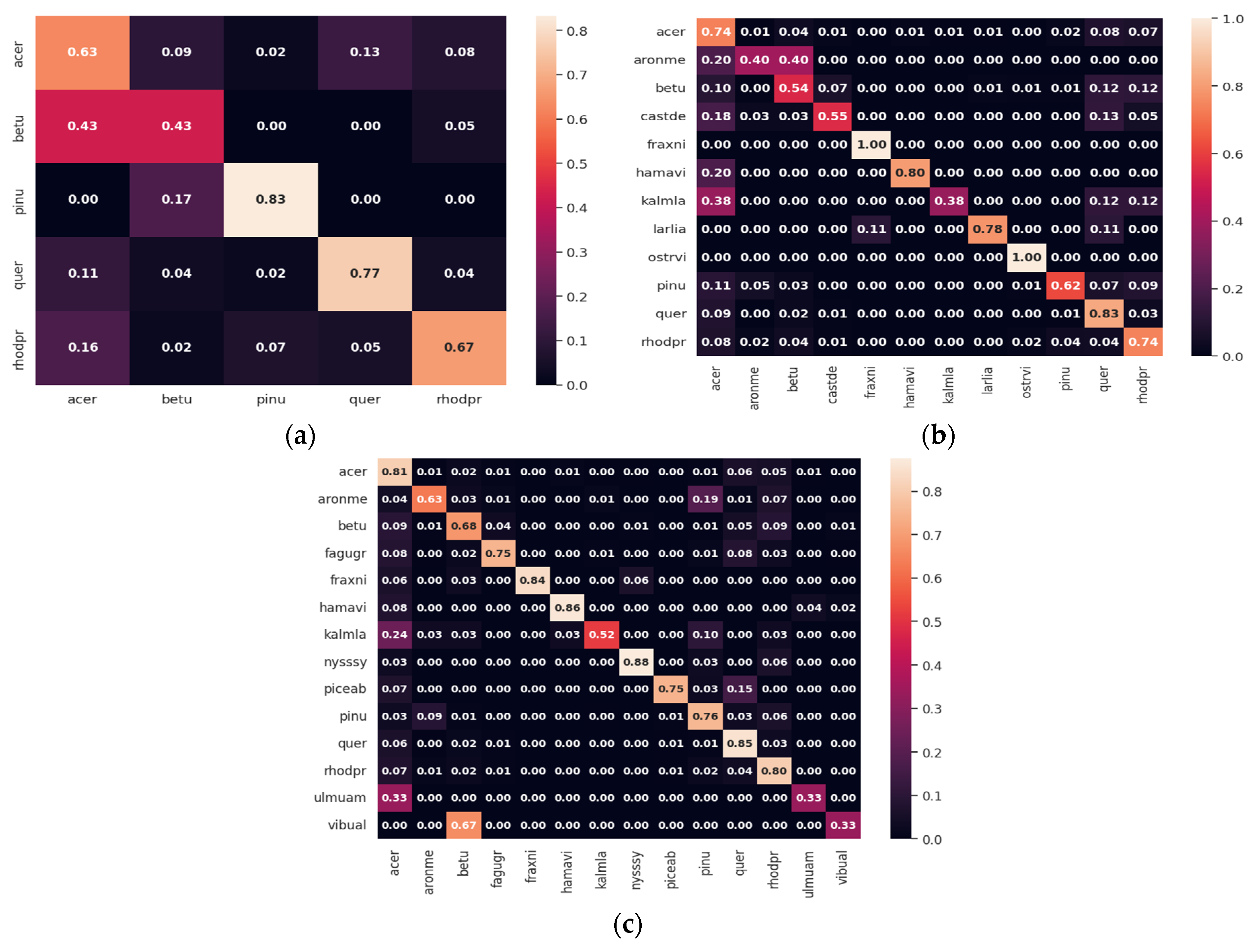
We utilized the confusion matrix to assess the accuracy of model predictions across different classes at a 10 nm spectral resolution and GSD = 5 m imagery. Figure 18 illustrates the confusion matrices for three scale resolutions: (a) 0.5X resolution; (b) 1X resolution; and (c) 2X resolution. It is important to note that the coarser image resolution led to under-classification (omission errors) due to inadequate samples of individual species. At 0.5X, 1X and 2X scale resolutions, the 1DCNN classifier demonstrated the successful classification of 5, 12, and 14 genus classes, respectively, out of a total of 24 classes in the dataset.
Notably, the 2X scale resolution showed higher precision and recall values per class. For instance, the acer class achieved 81% accuracy at 2X resolution, benefiting from a larger sample size and subsequent higher accuracies. At 1X resolution, intermediate recall and precision rates were observed with 74% accuracy, and at 0.5X resolution, only 63% accuracy was achieved for the acer class. However, at this 0.5X scale resolution, the CNN primarily identified dominant genus classes, whereas at 2X resolution, it was capable of identifying under-sampled classes. The results indicate that 2X scale resolution outperformed and can be considered as compatible with the accuracy achieved at GSD = 1 m.

3.5.2. Evaluating Different Scale Resolutions for Other Experimental Setups

In order to validate the consistency of the scale resolution impact on the classification performance, we also calculated the overall accuracy, kappa coefficient, F1 score, precision, and recall of the 1DCNN model (Table 14) at (i) GSD = 10 m and 10 nm spectral resolution; (ii) GSD = 10 m and 20 nm spectral resolution; (iii) GSD = 5 m and multispectral resolution (MS); and (iv) GSD = 10 m and multispectral resolution (MS).
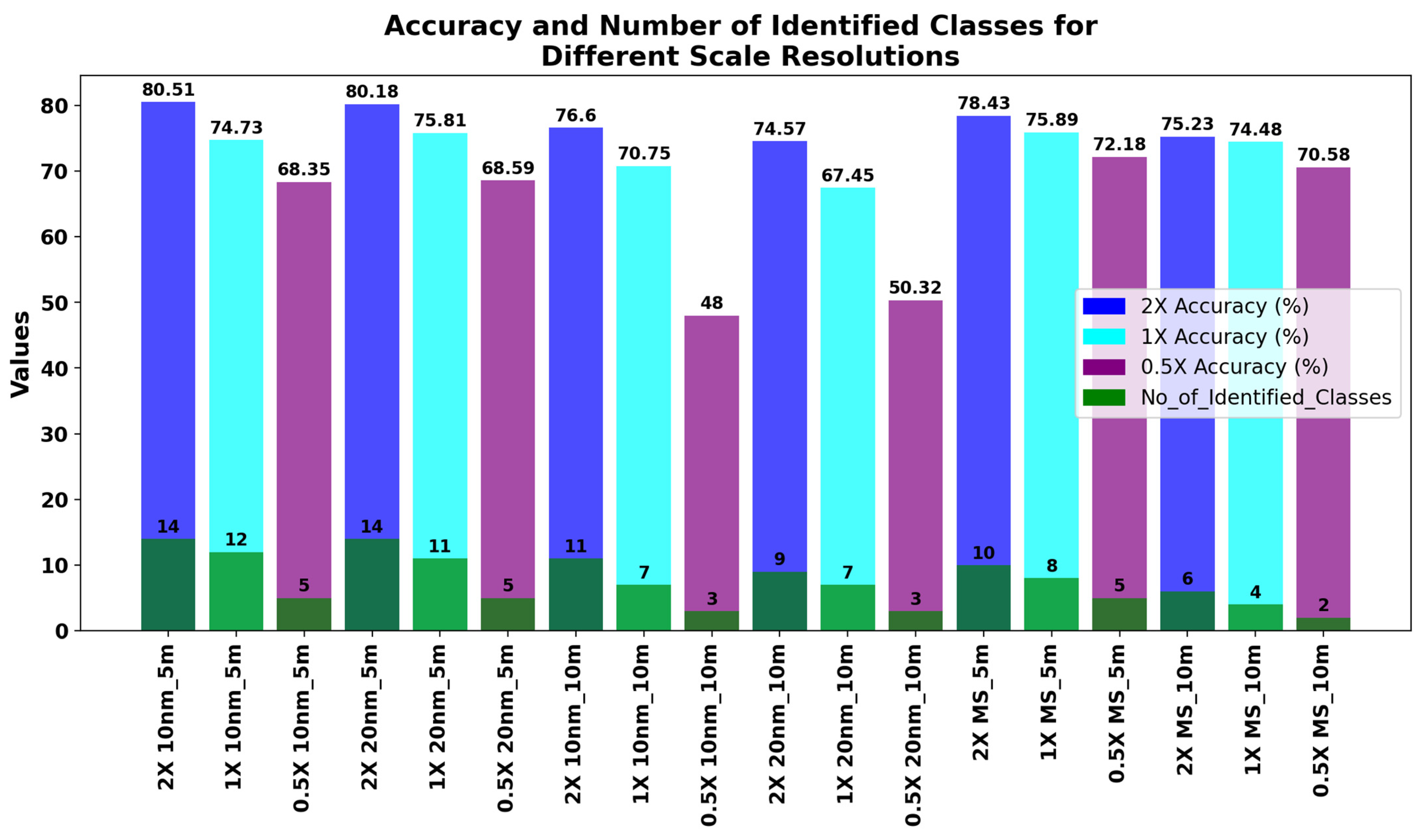
From Table 14, at 10 nm spectral resolution and GSD = 10 m (10 nm_10 m), for 2X, 1X, and 0.5X scale resolutions, we obtained overall accuracies of 76.60%, 70.75%, and 48%; kappa coefficients of 68.32%, 58.93%, and 22.32%; weighted precisions of 79%, 75%, and 52%; and recall rates of 77%, 71%, and 49%, respectively. At the same specification, the bar chart in Figure 19 demonstrates that the 1DCNN can identify eleven classes at 2Xresolution, seven at 1X resolution, and three at 0.5X resolution. On the other hand, when we reduce the spectral resolution to 20 nm while keeping the same GSD = 10 m (20 nm_10 m) (Table 14), the 1DCNN achieves overall accuracies of 74.57%, 67.45%, and 50.32%, with kappa coefficients of 65.57%, 53.90%, and 26.76%, along with nine, seven, and three identified classes for 2X, 1X, and 0.5X scale resolutions, respectively.
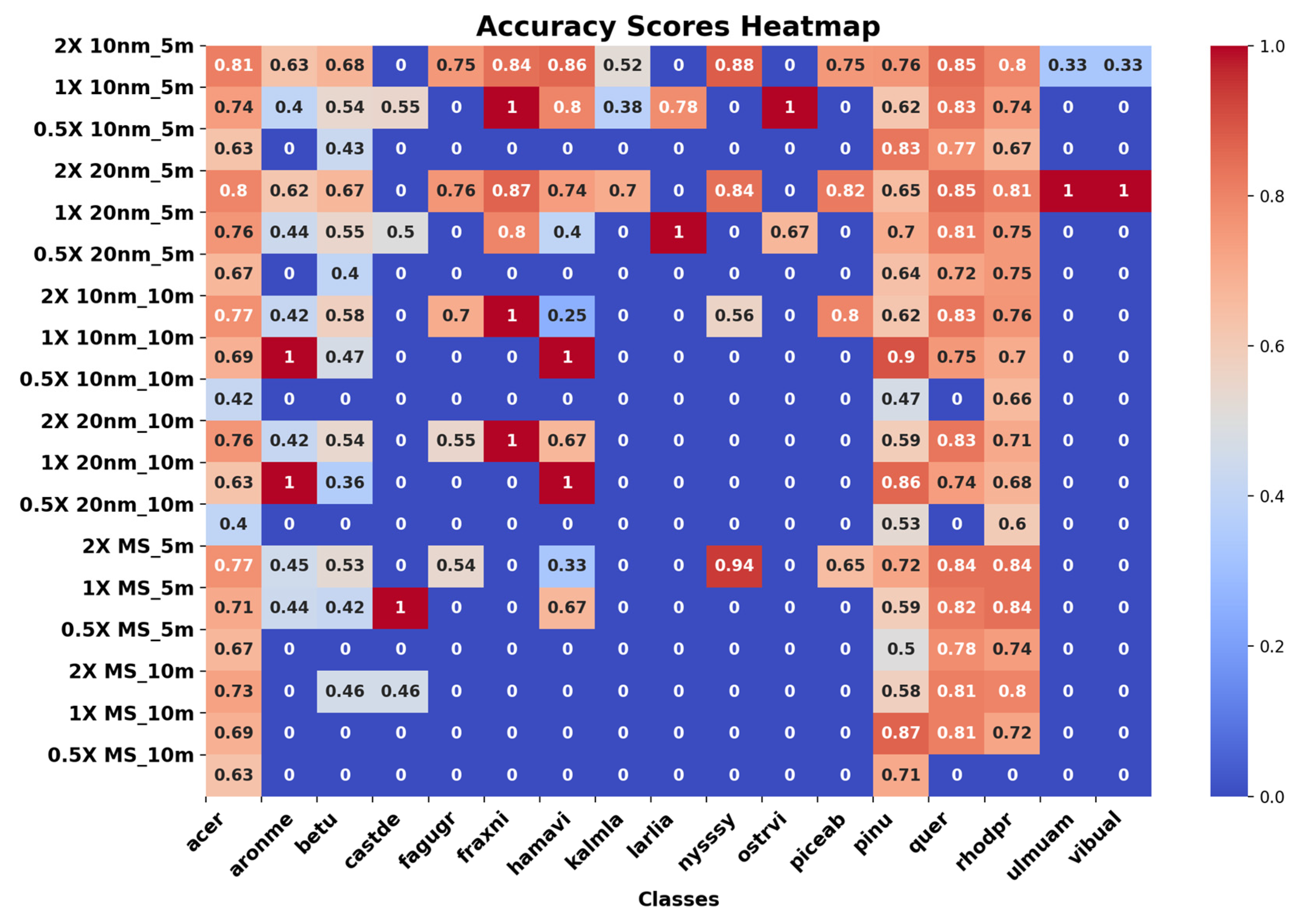
Table 14 also presents the results of the multispectral resolution scenario at 5 m and 10 m GSDs. At GSD 5 m with a wider bandpass (multispectral resolution) (MS_5 m), the 1DCNN achieved overall accuracies of 78.43%, 75.89%, and 72.18%, with corresponding kappa coefficients of 70.88%, 66.52%, and 60.32%, as well as ten, eight, and five identified genus-level species classes at 2X, 1X, and 0.5X resolutions, respectively. Similarly, at GSD = 10 m (MS_10 m) with 2X, 1X, and 0.5X resolutions, we obtained overall accuracies of 75.23%, 74.58%, and 70.58%; kappa coefficients of 65.73%, 62.96%, and 37.49%; and six, four, and two identified classes, respectively. Figure 19 summarizes the results for different combinations of sensor setups at various scale resolutions, allowing for a clear visual comparison. Additionally, Figure 20 displays the heatmap of per-class accuracy. It was concluded that a higher-scale resolution generally leads to better performance, but overall, the classification performance of the multispectral imagery is less affected by scale resolution when compared to imaging spectroscopy data.
We conclude from this analysis that the consideration of scale resolution is critical to future research directions, with the aim to enhance the accuracy and efficiency of classification tasks in diverse imaging scenarios. At 2X scale resolution, the simulated imaging sensors had a comparatively smaller pixel size of 100 microns, with a pixel array dimension of 1334 × 1104, while at 0.5X scale resolution, the pixel size was larger, measuring at 400 microns, with a pixel array dimension of 334 × 276. It is known that larger pixel sizes generally result in better signal-to-noise ratios (SNRs), assuming that the image sensors have the same fill factor of their pixels [55]. However, our results indicated that with a larger pixel size, we lost image content, which in turn affected the classification performance. Therefore, when designing a sensor, it is essential to consider these limitations and identify a balance between scale resolution, spatial resolution, spectral resolution and SNR in order to achieve the desired classification (or application-specific) performance. Moreover, the results significantly contribute to the broader field of study by advancing our understanding of the intricate relationships between spatial and spectral resolutions, as well as scale resolution, in the context of remote sensing of natural resources. The findings provide nuanced insights into the trade-offs involved in optimizing imaging systems for accurate classification tasks. This knowledge is crucial for informing the design and deployment of remote sensing technologies and guiding practitioners and policymakers in making informed decisions, thereby influencing the broader field of ecological monitoring, forestry management, and environmental assessment through advanced remote sensing methodologies.

4. Conclusions

Remote sensing technology is widely used by scientists to monitor and manage forest resources and assess ecosystem services, even though the various systems’ full potential and limitations arguably are not yet fully understood. Here, we demonstrated a simulation-based approach for modeling canopy-level reflectance from known leaf-level reflectance spectra and three-dimensional canopy structures in a virtual scene. The use of DIRSIG-simulated scene environments offers a promising solution to improve system understanding, given its flexibility to trace physical light transfer processes. We evaluated the impact of varying (i) spatial resolution, (ii) spectral resolution, and (iii) scale resolution on the classification performance of imaging spectrometers for remote sensing applications. A series of experiments, using simulated imaging spectroscopy data from a virtual Harvard Forest scene, systematically explored different combinations of spatial, spectral, and scale resolutions to understand their effects on identifying individual tree species. The findings revealed that spatial and scale resolutions particularly play a crucial role in species classification, with higher resolutions leading to improved accuracies and, critically, to more species classes being identified.
While examining the impact of spatial resolution, we observed that at higher spatial resolutions such as GSD = 1 m, accuracies as high as 83% are achievable, while at coarser spatial resolutions (GSD = 30 m), the classification accuracy can drop to as low as 50% for a complex forest scene. We also assessed the impact of spectral resolution at different spatial resolutions and contrasted the potential of a multispectral sensor for species classification. We observed that high spectral and spatial resolutions, e.g., GSDs = 1 m and 3 nm spectral resolutions, resulted in approximately 84% overall accuracy when using a 1D-CNN. However, this came with the cost of increased data volume and computational complexity. The multispectral resolution and GSD = 1 m approach, on the other hand, exhibited approximately 80% accuracy, thus making it a viable option for high-precision applications. It generally can be stated that, when using a higher spatial resolution, the most practical solution is to use a coarser spectral resolution sensor when a better species classification accuracy is the main objective. This statement obviously refers to our proxy application (species classification), while further studies into other applications are warranted. This study critically highlighted the careful consideration of scale resolution, which encompasses pixel pitch and sensor array dimensions, which is crucial in imaging sensor design for specific remote sensing applications. Remarkably, even at lower spatial and spectral resolutions, higher-scale resolutions with smaller pixel pitch and larger pixel array dimensions allowed the CNN to achieve up to 80% overall accuracy. Achieving accurate species classification while managing the trade-offs in sensor design, data storage, and computational requirements thus relies on finding the right balance between sensor scale, spatial, and spectral factors.
This research allowed us not only to assess the impact of sensor design on a specific application, but also to generate realistic imaging spectroscopy data for training and testing high-dimensional data algorithms. We were able to comprehensively assess the performance of CNN and SVM classifiers in a complex forest scene, thus observing how their effectiveness varied with different resolutions. The findings revealed that in a mixed forest scene, the 1DCNN outperformed both the HybridSN model and traditional SVM classifier in classifying vegetation species. Additionally, the study shed light on the challenges posed by a complex scene like that from Harvard Forest, where the presence of different species classes in varying proportions posed challenges, leading to an imbalanced dataset that directly impacted the classification performance.
This investigation into the impact of spatial, spectral, and scale resolutions on classification performance offers both practical and theoretical insights. The observed trade-off between spatial, spectral, and pixel sizes underscores the need for a careful balance in optimizing imaging systems. Although the results were promising, we acknowledge the limitations of working with synthetic data, which might introduce uncertainties in spectral sensitivity. Future research could benefit from validating these findings using real-world data, which could further enhance our understanding of the practical implications of sensor design for tree species classification. Building on this foundation, we can extend similar experiments to other imaging spectroscopy applications, such as exploring the impacts of ecosystem structural variability on reflectance products and investigating the impact of specific ecological changes on different sensor outputs. Researchers can enhance our understanding of sensor–landscape dynamics via physics-based simulations toward the optimization of remote sensing missions, thus guiding the design of future airborne and spaceborne missions. In practical applications, developing a new sensor for forestry or ecology studies is challenging. An effective approach involves identifying optimal system specifications and aligning these with existing sensors, thus emphasizing the need for theoretical optimization from a simulation study like this. This pragmatic strategy, though not ideal, is valuable given current technological constraints. Ultimately, the insights gained through these simulations will contribute to informed decision making and provide valuable guidance for practitioners and policymakers as well as foster progress in remote sensing technologies that impact diverse practical applications, such as forest management, biodiversity conservation, and ecological monitoring.

Author Contributions

Conceptualization, M.D.C. and J.v.A.; methodology, M.D.C. and J.v.A.; software, M.D.C.; validation, M.D.C.; formal analysis, M.D.C.; investigation, M.D.C.; data curation, M.D.C.; writing—original draft preparation, M.D.C.; writing—review and editing, J.v.A.; visualization, M.D.C.; supervision, J.v.A.; project administration, J.v.A.; funding acquisition, J.v.A. All authors have read and agreed to the published version of the manuscript.

Funding

This research was funded by the NASA ROSES (Research Opportunities for Space and Earth Science) BioSCape program (NASA grant number #80NSSC22K0831).

Data Availability Statement

Data are unavailable due to funding restrictions.

Acknowledgments

I acknowledge M. Grady Saunders and Kedar Patki for the technical support.

Conflicts of Interest

The authors declare no conflicts of interest.

References

  1. Nemani, R.R.; Running, S.W.; Pielke, R.A.; Chase, T.N. Global vegetation cover changes from coarse resolution satellite data. J. Geophys. Res. Atmos. 1996, 101, 7157–7162. [Google Scholar] [CrossRef]
  2. Myneni, R.B.; Dong, J.; Tucker, C.J.; Kaufmann, R.K.; Kauppi, P.E.; Liski, J.; Zhou, L.; Alexeyev, V.; Hughes, M. A large carbon sink in the woody biomass of Northern forests. Proc. Natl. Acad. Sci. USA 2001, 98, 14784–14789. [Google Scholar] [CrossRef] [PubMed]
  3. Swatantran, A.; Dubayah, R.; Roberts, D.; Hofton, M.; Blair, J.B. Mapping biomass and stress in the Sierra Nevada using lidar and hyperspectral data fusion. Remote Sens. Environ. 2011, 115, 2917–2930. [Google Scholar] [CrossRef]
  4. Ørka, H.O.; Dalponte, M.; Gobakken, T.; Naesset, E.; Ene, L.T. Characterizing forest species composition using multiple remote sensing data sources and inventory approaches. Scand. J. For. Res. 2013, 28, 677–688. [Google Scholar] [CrossRef]
  5. Fassnacht, F.E.; Latifi, H.; Stereńczak, K.; Modzelewska, A.; Lefsky, M.; Waser, L.T.; Straub, C.; Ghosh, A. Review of studies on tree species classification from remotely sensed data. Remote Sens. Environ. 2016, 186, 64–87. [Google Scholar] [CrossRef]
  6. Zhen, Z.; Quackenbush, L.J.; Zhang, L. Trends in Automatic Individual Tree Crown Detection and Delineation—Evolution of LiDAR Data. Remote Sens. 2016, 8, 333. [Google Scholar] [CrossRef]
  7. Zemek, F. Airborne Remote Sensing: Theory and Practice in Assessment of Terrestrial Ecosystems; Global Change Research Centre AS CR: Brno, Czech Republic, 2014. [Google Scholar]
  8. Wang, K.; Wang, T.; Liu, X. A Review: Individual Tree Species Classification Using Integrated Airborne LiDAR and Optical Imagery with a Focus on the Urban Environment. Forests 2019, 10, 1. [Google Scholar] [CrossRef]
  9. Immitzer, M.; Atzberger, C.; Koukal, T. Tree Species Classification with Random Forest Using Very High Spatial Resolution 8-Band WorldView-2 Satellite Data. Remote Sens. 2012, 4, 2661–2693. [Google Scholar] [CrossRef]
  10. Cochrane, M. Using vegetation reflectance variability for species level classification of hyperspectral data. Int. J. Remote Sens. 2000, 21, 2075–2087. [Google Scholar] [CrossRef]
  11. Van Leeuwen, M.; Frye, H.A.; Wilson, A.M. Understanding limits of species identification using simulated imaging spectroscopy. Remote Sens. Environ. 2021, 259, 112405. [Google Scholar] [CrossRef]
  12. Huang, J.; Wang, Y.; Zhang, D.; Yang, L.; Xu, M.; He, D.; Zhuang, X.; Yao, Y.; Hou, J. Design and demonstration of airborne imaging system for target detection based on area-array camera and push-broom hyperspectral imager. Infrared Phys. Technol. 2021, 116, 103794. [Google Scholar] [CrossRef]
  13. Nalepa, J.; Myller, M.; Cwiek, M.; Zak, L.; Lakota, T.; Tulczyjew, L.; Kawulok, M. Towards on-board hyperspectral satellite image segmentation: Understanding robustness of deep learning through simulating acquisition conditions. Remote Sens. 2021, 13, 1532. [Google Scholar] [CrossRef]
  14. Verrelst, J.; Camps-Valls, G.; Muñoz-Marí, J.; Rivera, J.P.; Veroustraete, F.; Clevers, J.G.; Moreno, J. Optical remote sensing and the retrieval of terrestrial vegetation bio-geophysical properties—A review. ISPRS J. Photogramm. Remote Sens. 2015, 108, 273–290. [Google Scholar] [CrossRef]
  15. Verrelst, J.; Rivera, J.P.; Moreno, J.; Camps-Valls, G. Gaussian processes uncertainty estimates in experimental Sentinel-2 LAI and leaf chlorophyll content retrieval. ISPRS J. Photogramm. Remote Sens. 2013, 86, 157–167. [Google Scholar] [CrossRef]
  16. Xu, X.; Lu, J.; Zhang, N.; Yang, T.; He, J.; Yao, X.; Cheng, T.; Zhu, Y.; Cao, W.; Tian, Y. Inversion of rice canopy chlorophyll content and leaf area index based on coupling of radiative transfer and Bayesian network models. ISPRS J. Photogramm. Remote Sens. 2019, 150, 185–196. [Google Scholar] [CrossRef]
  17. Nur, N.B.; Bachmann, C.M. Comparison of soil moisture content retrieval models utilizing hyperspectral goniometer data and hyperspectral imagery from an unmanned aerial system. J. Geophys. Res. Biogeosci. 2023, 128, e2023JG007381. [Google Scholar] [CrossRef]
  18. Masemola, C.; Cho, M.A.; Ramoelo, A. Towards a semi-automated mapping of Australia native invasive alien Acacia trees using Sentinel-2 and radiative transfer models in South Africa. ISPRS J. Photogramm. Remote Sens. 2020, 166, 153–168. [Google Scholar] [CrossRef]
  19. Miraglio, T.; Adeline, K.; Huesca, M.; Ustin, S.; Briottet, X. Joint Use of PROSAIL and DART for Fast LUT Building: Application to Gap Fraction and Leaf Biochemistry Estimations over Sparse Oak Stands. Remote Sens. 2020, 12, 2925. [Google Scholar] [CrossRef]
  20. Goodenough, A.A.; Brown, S.D. DIRSIG5: Next-generation remote sensing data and image simulation framework. IEEE J. Sel. Top. Appl. Earth Obs. Remote Sens. 2017, 10, 4818–4833. [Google Scholar] [CrossRef]
  21. Qi, J.; Xie, D.; Yin, T.; Yan, G.; Gastellu-Etchegorry, J.-P.; Li, L.; Zhang, W.; Mu, X.; Norford, L.K. LESS: LargE-Scale remote sensing data and image simulation framework over heterogeneous 3D scenes. Remote Sens. Environ. 2019, 221, 695–706. [Google Scholar] [CrossRef]
  22. Wald, I.; Woop, S.; Benthin, C.; Johnson, G.S.; Ernst, M. Embree: A kernel framework for efficient CPU ray tracing. ACM Trans. Graph. (TOG) 2014, 33, 1–8. [Google Scholar] [CrossRef]
  23. North, P.R. Three-dimensional forest light interaction model using a Monte Carlo method. IEEE Trans. Geosci. Remote Sens. 1996, 34, 946–956. [Google Scholar] [CrossRef]
  24. Wu, J.; Van Aardt, J.; Asner, G.; Mathieu, R.; Kennedy-Bowdoin, T.; Knapp, D.; Wessels, K.; Erasmus, B.; Smit, I. Connecting the dots between laser waveforms and herbaceous biomass for assessment of land degradation using small-footprint waveform lidar data. In Proceedings of the 2009 IEEE International Geoscience and Remote Sensing Symposium, Cape Town, South Africa, 12–17 July 2009; pp. II-334–II-337. [Google Scholar]
  25. Wu, J.; Van Aardt, J.; Asner, G.P. A comparison of signal deconvolution algorithms based on small-footprint LiDAR waveform simulation. IEEE Trans. Geosci. Remote Sens. 2011, 49, 2402–2414. [Google Scholar] [CrossRef]
  26. Wu, J.; Van Aardt, J.; McGlinchy, J.; Asner, G.P. A robust signal preprocessing chain for small-footprint waveform lidar. IEEE Trans. Geosci. Remote Sens. 2012, 50, 3242–3255. [Google Scholar] [CrossRef]
  27. Romanczyk, P.; van Aardt, J.; Cawse-Nicholson, K.; Kelbe, D.; McGlinchy, J.; Krause, K. Assessing the impact of broadleaf tree structure on airborne full-waveform small-footprint LiDAR signals through simulation. Can. J. Remote Sens. 2013, 39, S60–S72. [Google Scholar] [CrossRef]
  28. Yao, W.; Kelbe, D.; Leeuwen, M.V.; Romanczyk, P.; Aardt, J.V. Towards an improved LAI collection protocol via simulated and field-based PAR sensing. Sensors 2016, 16, 1092. [Google Scholar] [CrossRef]
  29. Yao, W.; van Aardt, J.; van Leeuwen, M.; Kelbe, D.; Romanczyk, P. A simulation-based approach to assess subpixel vegetation structural variation impacts on global imaging spectroscopy. IEEE Trans. Geosci. Remote Sens. 2018, 56, 4149–4164. [Google Scholar] [CrossRef]
  30. Maschler, J.; Atzberger, C.; Immitzer, M. Individual tree crown segmentation and classification of 13 tree species using airborne hyperspectral data. Remote Sens. 2018, 10, 1218. [Google Scholar] [CrossRef]
  31. Ferreira, M.P.; Zortea, M.; Zanotta, D.C.; Shimabukuro, Y.E.; de Souza Filho, C.R. Mapping tree species in tropical seasonal semi-deciduous forests with hyperspectral and multispectral data. Remote Sens. Environ. 2016, 179, 66–78. [Google Scholar] [CrossRef]
  32. Fricker, G.A.; Ventura, J.D.; Wolf, J.A.; North, M.P.; Davis, F.W.; Franklin, J. A convolutional neural network classifier identifies tree species in mixed-conifer forest from hyperspectral imagery. Remote Sens. 2019, 11, 2326. [Google Scholar] [CrossRef]
  33. Ghosh, A.; Fassnacht, F.E.; Joshi, P.K.; Koch, B. A framework for mapping tree species combining hyperspectral and LiDAR data: Role of selected classifiers and sensor across three spatial scales. Int. J. Appl. Earth Obs. Geoinf. 2014, 26, 49–63. [Google Scholar] [CrossRef]
  34. Guo, X.; Li, H.; Jing, L.; Wang, P. Individual tree species classification based on convolutional neural networks and multitemporal high-resolution remote sensing images. Sensors 2022, 22, 3157. [Google Scholar] [CrossRef] [PubMed]
  35. Hsieh, T.-H.; Kiang, J.-F. Comparison of CNN algorithms on hyperspectral image classification in agricultural lands. Sensors 2020, 20, 1734. [Google Scholar] [CrossRef] [PubMed]
  36. Wible, R.; Patki, K.; Krause, K.; van Aardt, J. Toward a Definitive Assessment of the Impact of Leaf Angle Distributions on LiDAR Structural Metrics. In Proceedings of the SilviLaser Conference 2021, Vienna, Austria, 28–30 September 2021; pp. 307–309. [Google Scholar]
  37. Schott, J.R.; Brown, S.D.; Raqueno, R.V.; Gross, H.N.; Robinson, G. An advanced synthetic image generation model and its application to multi/hyperspectral algorithm development. Can. J. Remote Sens. 1999, 25, 99–111. [Google Scholar] [CrossRef]
  38. Schott, J.R.; Raqueno, R.V.; Salvaggio, C. Incorporation of a time-dependent thermodynamic model and a radiation propagation model into IR 3D synthetic image generation. Opt. Eng. 1992, 31, 1505–1516. [Google Scholar] [CrossRef]
  39. Green, R.O.; Conel, J.E.; Roberts, D.A. Estimation of aerosol optical depth, pressure elevation, water vapor, and calculation of apparent surface reflectance from radiance measured by the airborne visible/infrared imaging spectrometer. In Proceedings of the Imaging Spectrometry of the Terrestrial Environment, Orlando, FL, USA, 11–16 April 1993; pp. 2–11. [Google Scholar]
  40. Sanders, L.C.; Schott, J.R.; Raqueno, R. A VNIR/SWIR atmospheric correction algorithm for hyperspectral imagery with adjacency effect. Remote Sens. Environ. 2001, 78, 252–263. [Google Scholar] [CrossRef]
  41. Conel, J.E.; Green, R.O.; Vane, G.; Bruegge, C.J.; Alley, R.E.; Curtiss, B.J. AIS-2 radiometry and a comparison of methods for the recovery of ground reflectance. In Proceedings of the 3rd Airborne Imaging Spectrometer Data Analysis Workshop, Pasadena, CA, USA, 2–4 June 1987. [Google Scholar]
  42. Kotawadekar, R. 9—Satellite data: Big data extraction and analysis. In Artificial Intelligence in Data Mining; Binu, D., Rajakumar, B.R., Eds.; Academic Press: Cambridge, MA, USA, 2021; pp. 177–197. [Google Scholar] [CrossRef]
  43. Malenovsky, Z. Quantitative Remote Sensing of Norway Spruce (Picea Abies (L.) Karst.): Spectroscopy from Needles to Crowns to Canopies; Wageningen University and Research: Wageningen, The Netherlands, 2006. [Google Scholar]
  44. Safonova, A.; Tabik, S.; Alcaraz-Segura, D.; Rubtsov, A.; Maglinets, Y.; Herrera, F. Detection of fir trees (Abies sibirica) damaged by the bark beetle in unmanned aerial vehicle images with deep learning. Remote Sens. 2019, 11, 643. [Google Scholar] [CrossRef]
  45. Egli, S.; Höpke, M. CNN-based tree species classification using high resolution RGB image data from automated UAV observations. Remote Sens. 2020, 12, 3892. [Google Scholar] [CrossRef]
  46. Agarap, A.F. Deep learning using rectified linear units (relu). arXiv 2018, arXiv:1803.08375. [Google Scholar]
  47. Gulli, A.; Pal, S. Deep Learning with Keras; Packt Publishing Ltd.: Birmingham, UK, 2017. [Google Scholar]
  48. Srivastava, N.; Hinton, G.; Krizhevsky, A.; Sutskever, I.; Salakhutdinov, R. Dropout: A simple way to prevent neural networks from overfitting. J. Mach. Learn. Res. 2014, 15, 1929–1958. [Google Scholar]
  49. Ruder, S. An overview of gradient descent optimization algorithms. arXiv 2016, arXiv:1609.04747. [Google Scholar]
  50. Melgani, F.; Bruzzone, L. Classification of hyperspectral remote sensing images with support vector machines. IEEE Trans. Geosci. Remote Sens. 2004, 42, 1778–1790. [Google Scholar] [CrossRef]
  51. Roy, S.K.; Krishna, G.; Dubey, S.R.; Chaudhuri, B.B. HybridSN: Exploring 3-D–2-D CNN feature hierarchy for hyperspectral image classification. IEEE Geosci. Remote Sens. Lett. 2019, 17, 277–281. [Google Scholar] [CrossRef]
  52. Rodarmel, C.; Shan, J. Principal component analysis for hyperspectral image classification. Surv. Land Inf. Sci. 2002, 62, 115–122. [Google Scholar]
  53. Nweke, H.F.; Teh, Y.W.; Al-Garadi, M.A.; Alo, U.R. Deep learning algorithms for human activity recognition using mobile and wearable sensor networks: State of the art and research challenges. Expert Syst. Appl. 2018, 105, 233–261. [Google Scholar] [CrossRef]
  54. Wagle, S.A.; Harikrishnan, R.; Ali, S.H.M.; Faseehuddin, M. Classification of plant leaves using new compact convolutional neural network models. Plants 2021, 11, 24. [Google Scholar] [CrossRef] [PubMed]
  55. Mather, P.M.; Koch, M. Computer Processing of Remotely-Sensed Images: An Introduction; John Wiley & Sons: Hoboken, NJ, USA, 2011. [Google Scholar]
  56. Zhang, H.; Zhang, L.; Shen, H. A super-resolution reconstruction algorithm for hyperspectral images. Signal Process. 2012, 92, 2082–2096. [Google Scholar] [CrossRef]
  57. Kokaly, R.F.; Clark, R.N. Spectroscopic determination of leaf biochemistry using band-depth analysis of absorption features and stepwise multiple linear regression. Remote Sens. Environ. 1999, 67, 267–287. [Google Scholar] [CrossRef]
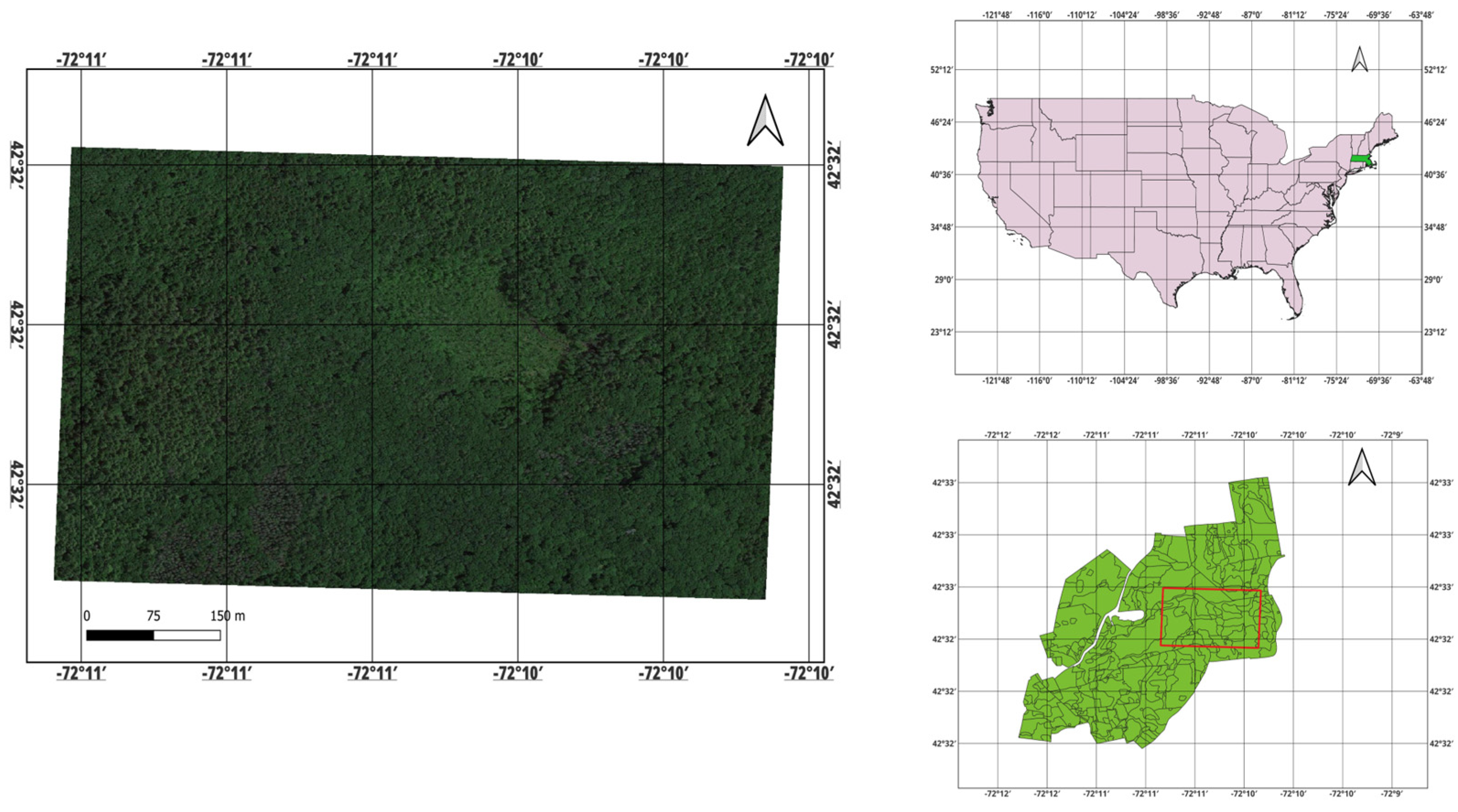
Figure 1. Study area in Harvard Forest—a National Ecological Observatory Network (NEON) Research Forest located in Petersham, MA, USA. The red border indicates the boundary of the area and the view of the area from Google Earth Engine is depicted in the gridded white raster box. This figure is drawn in QGIS software version 3.28.3.
Remotesensing 16 00498 g001
Figure 2. Generalized reflectance curve of the various plant species as mentioned in Table 1. These were used during the development of the virtual scene of the Harvard Forest study area.
Remotesensing 16 00498 g002
Figure 3. Flow diagram to illustrate the development of the virtual Harvard Forest scene. All the input parameters were fed into the DIRSIG scene geometry builder to obtain a comprehensive scene.
Remotesensing 16 00498 g003
Figure 4. A complete flowchart that describes the simulation process for a Harvard Forest scene using the DIRSIG simulator: (left) 3D scene built using geometric and structural properties, (middle-top) integrated with scene optical properties and (middle-bottom) platform/sensing system specifics to (right) render an output scene for different sensing modalities (e.g., multispectral, spectrometer, or LiDAR).
Remotesensing 16 00498 g004
Figure 5. (a) Two bright panels and two dark panels were placed at the corners and used as the reference objects for ELM-based atmospheric compensation. (b) Mean reflectance spectra of the simulated scene after the atmospheric compensation. The gap in the reflectance spectra is due to the removal of the water absorption feature around 1950 nm.
Remotesensing 16 00498 g005
Figure 6. Fundamental geometrical illustration of an airborne or spaceborne imaging system: field-of-view (FOV), instantaneous field-of-view (IFOV), and ground sampling distance (GSD) (picture is not drawn in accurate scale).
Remotesensing 16 00498 g006
Figure 7. An illustration of spectral resolution; Gaussian-shaped FWHM (full width at half maximum) with an extent from λ m a x   t o   λ m i n and spectral sampling of imaging spectroscopy data. One should note that the pursuit of finer spectral resolution, by employing over-sampling, comes at the cost of information redundancy, since neighboring spectral bands capture repetitive (correlated) data [43].
Remotesensing 16 00498 g007
Figure 8. Illustration of different scale resolution image sensors. From left to right, the images demonstrate the generation of low, medium, and high pixel density tree images, respectively, all with the same sensor width area.
Remotesensing 16 00498 g008
Figure 9. The 1DCNN model architecture used in this study. The model consists of two consecutive 1D convolutional and pooling layers, dropout layers, and fully connected/dense layers. The output layer is equal to ground truth label classes, and assigns probabilities to each of the possible classes to classify the input image into one of the specified categories.
Remotesensing 16 00498 g009
Figure 10. An example of high-resolution rendered scene of Harvard Forest, generated using the DIRSIG model, captured at nadir and at a 1000 m flight altitude. Here, we depict the forest scene in true color (red—638 nm; green—548 nm; and blue—470 nm).
Remotesensing 16 00498 g010
Figure 11. At-nadir simulated imagery for varying GSDs. As the GSD values increase, the images exhibit an obvious decrease in resolution. This visual representation highlights the relationship between GSD and image clarity, emphasizing the importance of choosing an appropriate GSD for obtaining finer details and higher image quality, depending on remote sensing applications. Subtle difference of colors in the figures is from QGIS version 3.28.3 software.
Remotesensing 16 00498 g011
Figure 12. Ground truth images simulated by DIRSIG for various ground sampling distance (GSD) values, with each color representing a distinct genus-level plant species/class level.
Remotesensing 16 00498 g012
Figure 13. Bar chart of the accuracy and number of classes identified by different classifiers. The ground sampling distance ranged from 1 to 30 m.
Remotesensing 16 00498 g013
Figure 14. Heatmap of recall/accuracy per class for different-resolution imagery for different classifiers. It visually represents the performance of each class in terms of recall (sensitivity) and accuracy, thereby providing insight into the effectiveness of different classifiers under different resolution conditions.
Remotesensing 16 00498 g014
Figure 15. (a) The bar chart presents the accuracy and number of classes identified by the 1DCNN classifier. (b) Heatmap of recall/accuracy per class for different spectral resolution imagery GSD = 1 m.
Remotesensing 16 00498 g015
Figure 16. (a) The bar chart presents the accuracy and number of classes identified by the 1DCNN classifier. (b) Heatmap of recall/accuracy per class for different-spectral-resolution imagery at GSD = 5 m.
Remotesensing 16 00498 g016
Figure 17. (a) The bar chart presents the accuracy and number of classes identified by the 1DCNN classifier. (b) Heatmap of recall/accuracy per class for different spectral resolution imagery at GSD = 10 m.
Remotesensing 16 00498 g017
Figure 18. Confusion matrix of 10 nm spectral resolution and GSD = 5 m imagery at (a) 0.5X resolution; (b) 1X resolution; and (c) 2X resolution. Note that the diagonal elements represent correct predictions, and off-diagonal elements represent errors. Coarser scale (0.5X) resolution led to under-classification (omission errors) due to inadequate samples of individual species, highlighting the significance of adequate scale resolution for accurate classification. It also provides us the insight that the number of identified classes decreased with reduced scale resolution.
Remotesensing 16 00498 g018
Figure 19. The accuracy and number of classes identified by the 1DCNN classifier, as well as overall accuracy for varying scale resolutions at different experimental setups. Note that “2X_10 nm_5 m” implies that the imagery was acquired at a 10 nm spectral bandpass, GSD = 5 m, and a 2X scale resolution.
Remotesensing 16 00498 g019
Figure 20. A heatmap that visually represents the performance of each class in terms of recall (sensitivity) and accuracy, providing insight into the effectiveness of the 1DCNN classifier under different scale resolutions. Note that “1X 10 nm_5 m” implies 1X scale resolution at 10 nm spectral bandpass and GSD = 5 m, while “MS” represents the multispectral sensor case.
Remotesensing 16 00498 g020
Table 1. The taxonomy information and list of sample plant species in Harvard Forest.
ClassScientific NameGenusCommon NameTypeNumber of Individuals
acerAcer pennsylvanicumAcerMoosewood MapleTree354
Acer rubrumAcerRed MapleTree10,760
aronmeAronia melanocarpaAroniaBlack ChokeberrySubcanopy413
betualBetula alleghaniensisBetulaYellow BirchSubcanopy4452
Betula lentaBetulaBlack BirchTree1479
Betula papyriferaBetulaPaper BirchTree711
Betula populifoliaBetulaGrey BirchTree131
castdeCastanea dentataCastaneaAmerican ChestnutSubcanopy782
fagugrFagus grandifoliaFagusBeechTree3879
fraxniFraxinus nigraFraxinusBlack AshTree38
hamaviHamamelis virginianaHamamelisWitch-hazelSubcanopy1967
ilexveIlex verticillataIlexWinterberrySubcanopy9875
kalmlaKalmia latifoliaKalmiaMountain LaurelSubcanopy3929
larilaLarix laricinaLarixTamarack Subcanopy1
lyonliLyonia ligustrinaLyoniaMaleberrySubcanopy1178
nemomuNemopanthus mucronatusNemopanthusMountain HolleySubcanopy599
nysssyNyssa sylvaticaNyssaTupeloTree181
ostrviOstrya virginianaOstryaHornbeamTree24
piceabPicea abiesPiceaNorway SpruceTree1458
pinuPinus resinosaPinusRed PineTree973
Pinus strobusPinusEastern White PineTree3070
querQuercus albaQuercusWhite OakTree46
Quercus rubraQuercusNorthern Red OakTree4122
rhodprRhododendron prinophyllumRhododendronRhododendronSubcanopy127
tsugcaTsuga canadensisTsugaEastern HemlockTree24,266
ulmuamUlmus americanaUlmusElmTree1
vacccoVaccinium corymbosumVacciniumBlueberry bushSubcanopy3533
vibualViburnum alnifoliumViburnumHobblebushSubcanopy76
soil---
bark---
Table 2. Summary of the imaging spectrometer data used in this paper.
Hyperspectral ImagerAVIRIS Classic
Spectral Bands224
Spectral Range380–2500
Spectral Sampling10 nm FWHM (Gaussian)
Pixel Array667 × 552
Pixel Size200 microns
Focal Length197.60 mm
Flying Height1–30 km
GSD1–30 m
Table 3. Demonstration of spectral sampling and the total number of bands.
Spectral SamplingTotal No. of Bands
3 nm714
5 nm425
7 nm306
10 nm224
12 nm178
15 nm143
17 nm126
20 nm108
25 nm83
30 nm69
Multispectral (MS)8
Table 4. Scale resolution, corresponding pixel array, and pixel sizes used for the simulation.
Scale ResolutionPixel Array DimensionPixel Size/Pitch (Microns)
0.5X334 × 276400.00
1X667 × 552200.00
2X1334 × 1104100.00
Table 5. Split training and test set for the imagery of different ground sampling distances.
GSDNumber of Samples (Pixels)Total
TrainTest
1.0 m 216,561 92,812 309,373
1.5 m 93,618 40,122 133,740
2.0 m 51,825 22,211 74,036
2.5 m 32,738 14,031 46,769
3.0 m 22,538 9660 32,198
4.0 m 12,428 5327 17,755
5.0 m 7849 3365 11,214
10 m 1770 759 2529
20 m 350 150 500
30 m 140 61 201
Table 6. Summary of results from the 1DCNN model reporting the overall accuracy, precision, recall, and F-Score for different spatial resolutions of imaging spectroscopy data.
GSDOverall
Accuracy (OA)
(%)
Kappa
Coefficient (%)
F1 Score
(%)
PrecisionRecall
Macro
Average (%)
Weighted
Average (%)
Macro
Average (%)
Weighted
Average (%)
1.0 m 82.83 77.51 83 40 85 59 83
2.0 m 81.41 75.35 81 35 83 46 81
3.0 m 80.72 74.18 81 38 82 56 81
4.0 m 78.05 70.56 78 34 80 42 78
5.0 m 75.76 65.89 75 37 77 56 75
10 m 70.35 58.17 70 27 76 43 70
20 m 67.33 37.58 67 16 79 15 67
30 m 54.09 18.70 54 21 62 18 54
Table 7. Summary of results from the HybridSN model reporting the overall accuracy, precision, recall, and F-Score for different spatial resolutions of imaging spectroscopy data.
GSDOverall
Accuracy (OA) (%)
Kappa
Coefficient (%)
F1 Score
(%)
PrecisionRecall
Macro
Average (%)
Weighted
Average (%)
Macro
Average (%)
Weighted
Average (%)
1.0 m 76.94 69.81 77 45 76 33 77
2.0 m 73.55 64.85 74 42 72 29 74
3.0 m 69.34 58.70 69 40 68 24 69
4.0 m 60.87 46.90 61 37 59 20 61
5.0 m 57.12 41.51 57 27 55 23 57
10 m 50.98 31.47 51 26 48 24 51
20 m 55.33 16.97 55 12 49 14 55
30 m 57.37 30.37 57 24 59 24 57
Table 8. Summary of results from the PCA-SVM reporting the overall accuracy, precision, recall, and F-Score for different spatial resolutions of imaging spectroscopy data.
GSDOverall
Accuracy (OA) (%)
Kappa
Coefficient (%)
F1 Score (%)PrecisionRecall
Macro
Average (%)
Weighted
Average (%)
Macro
Average (%)
Weighted
Average (%)
1.0 m 68.62 57.33 68.62 0.28 671569
2.0 m 67.73 55.41 67.73 23 65 14 68
3.0 m 65.82 52.37 65.82 22 60 15 66
4.0 m 62.26 47.23 62.26 17 56 13 62
5.0 m 61.57 45.72 61.57 18 53 17 62
10 m 55.33 35.96 55.33 14 48 16 55
20 m 50.66 10.00 50.66 7 26 14 51
30 m 55.73 15.01 55.73 21 50 23 56
Table 9. A summary of the 1DCNN results, reporting the overall accuracy, precision, recall, and F-Score for different spectral resolutions for GSD = 1 m of imaging spectroscopy data.
BandpassOverall
Accuracy (OA) (%)
Kappa
Coefficient (%)
F1 Score
(%)
PrecisionRecall
Macro
Average (%)
Weighted
Average (%)
Macro
Average (%)
Weighted
Average (%)
3 nm 84.08 79.46 84 48 85 63 84
5 nm 83.35 78.32 83 45 84 58 83
7 nm 82.90 77.67 83 44 84 56 83
10 nm 82.83 77.51 83 40 85 59 83
12 nm 82.56 77.22 83 40 84 55 83
15 nm 82.18 76.76 82 40 84 55 82
17 nm 81.81 76.19 82 38 84 55 82
20 nm 81.80 76.18 82 37 84 53 84
25 nm 81.37 75.65 81 36 84 53 81
30 nm 81.23 75.39 81 35 84 51 81
MS 79.98 73.56 80 31 83 42 80
Table 10. A summary of the 1DCNN results reporting the overall accuracy, precision, recall, and F1 score for different spectral resolutions for GSD = 5 m of imaging spectroscopy data.
BandpassOverall
Accuracy (OA) (%)
Kappa
Coefficient (%)
F1 Score
(%)
PrecisionRecall
Macro
Average (%)
Weighted
Average (%)
Macro
Average (%)
Weighted
Average (%)
3 nm 76.61 68.20 77 37 80 57 77
5 nm 76.67 68.52 77 35 79 54 77
7 nm 75.88 67.22 76 31 80 43 76
10 nm 74.83 65.84 75 41 77 64 75
12 nm 76.72 68.55 77 37 79 53 77
15 nm 74.84 65.98 75 35 78 56 75
17 nm 75.13 66.18 75 31 78 46 75
20 nm 75.63 67.11 76 31 79 50 76
25 nm 73.93 64.36 74 32 79 54 74
30 nm 72.84 62.49 72 25 77 31 72
MS 75.89 66.52 76 26 83 39 76
Table 11. A summary of the 1DCNN results reporting the overall accuracy, precision, recall, and F1 score for different spectral resolutions for GSD = 10 m of imaging spectroscopy data.
BandpassOverall
Accuracy (OA) (%)
Kappa
Coefficient (%)
F1 Score
(%)
PrecisionRecall
Macro
Average (%)
Weighted
Average (%)
Macro
Average (%)
Weighted
Average (%)
3 nm 71.03 60.01 71 25 73 29 71
5 nm 71.07 59.43 71 26 71 31 71
7 nm 69.43 57.00 69 26 75 29 69
10 nm 70.75 58.93 71 30 75 50 71
12 nm 69.21 56.74 69 27 74 42 69
15 nm 67.42 54.34 67 27 73 38 67
17 nm 69.54 57.41 70 29 74 39 70
20 nm 67.45 53.90 67 26 73 44 67
25 nm 66.67 52.78 67 25 73 36 67
30 nm 66.05 52.06 66 25 72 31 66
MS 74.48 62.96 74 27 82 28 74
Table 12. A summary of the 1DCNN results, reporting the overall accuracy, precision, recall, and F-Score for different scale resolutions at 10 nm bandpass/spectral resolution and GSD = 5 m (10 nm_5 m) and 20 nm bandpass/spectral resolution and GSD = 5 m (20 nm_5 m) for imaging spectroscopy data.
Scale ResolutionOverall
Accuracy (OA) (%)
Kappa
Coefficient (%)
F1 Score
(%)
PrecisionRecall
Macro
Average (%)
Weighted
Average (%)
Macro
Average (%)
Weighted
Average (%)
2X 10 nm_5 m 81.00 74.23 81 40 82 55 81
1X 10 nm_5 m 74.73 65.84 75 41 77 64 75
0.5X 10 nm_5 m 68.35 55.20 68 22 75 28 68
2X 20 nm_5 m 80.18 73.57 80 38 82 62 80
1X 20 nm_5 m 75.81 67.11 76 34 79 53 76
0.5X 20 nm_5 m 68.59 57.35 70 24 77 27 70
Table 13. Per-class pixel counts for different scale resolutions with 10 nm spectral resolution and GSD = 5 m.
Pixel Count per Class for Different Scale Resolutions
Class0.5X1X2X
acer 845 3603 15,010
aronme 18 108 599
bark - - 24
betu 178 746 3182
castde - 229 12
fagugr - - 989
fraxni 10 42 157
hamavi 12 67 343
kalmla 10 54 183
larlia 13 57 25
nysssy - - 216
ostrvi 13 71 4
piceab - - 365
pinu 98 421 1706
quer 882 3446 13,335
rhodpr 489 2340 9855
ulmuam 2 30 130
vibual - - 120
Table 14. A summary of the 1DCNN results, reporting the overall accuracy, precision, recall, and F-Score for different pixel elements at 10 nm bandpass/spectral resolution and GSD = 10 m (10 nm_10 m), 20 nm bandpass/spectral resolution and GSD = 10 m (20 nm_10 m), multispectral resolution and GSD = 5 m (MS_5 m), multispectral resolution and GSD = 10 m (MS_10 m) for imaging spectroscopy data.
Scale ResolutionOverall
Accuracy (OA) (%)
Kappa
Coefficient (%)
F1 Score
(%)
PrecisionRecall
Macro
Average (%)
Weighted
Average (%)
Macro
Average (%)
Weighted
Average (%)
2X 10 nm_10 m 76.60 68.32 77 33 79 49 77
1X 10 nm_10 m 70.75 58.93 71 30 75 50 71
0.5X 10 nm_10 m 48.00 22.32 49 20 52 19 49
2X 20 nm_10 m 74.57 65.57 75 33 78 43 75
1X 20 nm_10 m 67.45 53.90 67 26 73 44 73
0.5X 20 nm_10 m 50.32 26.67 50 21 54 19 50
2X MS_5 m 78.43 70.88 78 28 82 37 78
1X MS_5 m 75.89 66.52 76 26 83 39 76
0.5X MS_5 m 72.18 60.32 73 23 83 24 73
2X MS_10 m 75.23 65.73 75 27 81 29 75
1X MS_10 m 74.48 62.96 74 27 82 28 74
0.5X MS_10 m 70.58 37.49 68 20 75 19 68
Disclaimer/Publisher’s Note: The statements, opinions and data contained in all publications are solely those of the individual author(s) and contributor(s) and not of MDPI and/or the editor(s). MDPI and/or the editor(s) disclaim responsibility for any injury to people or property resulting from any ideas, methods, instructions or products referred to in the content.