Abstract
The Xiong’an New Area, following the precedent of the Shenzhen Special Economic Zone and Shanghai Pudong New Area, marks a significant development. This study introduces a method to optimize the feature variable selection for Sentinel-2 images from 2016 to 2022, aiming for precise land-use classification in Xiong’an using machine learning. The classification reveals substantial growth in the infrastructure and aquatic areas in Rongcheng and Xiongxian counties, outpacing Anxin from 2016 to 2022. The Remote Sensing-Based Ecological Index (RSEI) indicates a generally stable yet improving ecological landscape, especially in denser areas like Xiongxian and Rongcheng, aligning regional development with ecological enhancement. EOF analysis shows a spatial ecological division, with positive RSEI values in the western regions and negative values in the east, along with temporal fluctuations indicating a decline in the west and an increase in the east since 2017. Additionally, the RSEI’s short-cycle fluctuations emphasize the dynamic ecological state of the area, influenced by both long-term trends and transient factors.
1. Introduction
By integrating original spectra, spectral indices, and texture features, classification accuracy for land types can be remarkably enhanced [1,2]. However, this approach often leads to data redundancy. Optimum Index Factor (OIF) and Principal Component Analysis (PCA) can solve this problem. OIF is an effective method for selecting the most informative features from an image. Qi et al. demonstrated that the OIF method has stable performance and significant accuracy across different datasets [3]. The PCA, consistent with OIF, also aims to reduce data volume. Applying PCA transformation to data can significantly improve the accuracy of data classification [4,5]. The object-oriented approach to land-use/cover classification considers neighboring pixels as cohesive units, analyzing them based on multiple attributes like spectrum, shape, and texture [6,7]. This methodology diminishes the impact of mixed pixels, leading to the more precise extraction of surface feature information and offering both accuracy and efficiency in the process [8]. The LCLU classification method has been employed to assess the impacts of land cover changes on ecological environments, particularly in newly developed areas.
Established in April 2017, the Xiong’an New Area joins the ranks of China’s national-level development areas, following the Shenzhen Special Economic Zone (SZSEZ) and the Shanghai Pudong New Area (SHPNA). The founding of the Xiong’an New Area serves multiple purposes: to alleviate the non-capital functions of Beijing, to pioneer optimized development models for highly populated areas, to refine the spatial structure and urban layout of the Beijing–Tianjin–Hebei region, to foster innovation-driven growth engines, and to champion a sustainable ecological environment [9,10]. Since its inception, there has been a marked uptick in construction activity in the area [11]. The road network has nearly doubled over a span of three years [12]. Conversely, metrics show declines in cultivated lands, forests, and hydrophytes [6]. In recent years, research on the ecological aspects of the Xiong’an New Area has been extensive, with predominant themes centered on ecological quality [10,13,14,15], detection of land-use changes [11,12,16], projections for future land-use alterations [17,18], and studies of wetland [19,20,21].
The development of the Xiong’an New Area has the potential to substantially transform its landscapes. Effective urban construction planning is pivotal for the efficient management of the region’s land resources. As such, it becomes imperative to continuously monitor and assess both the changes in land cover/land use (LCLU) and their ecological implications. Current research on land use in the Xiong’an New Area is limited to the year 2020 [16], and although there is research on the ecology from 2021 [14], the observational indices used (NDVI/NDWI) are quite simple and do not reflect the real ecological situation of the Xiong’an New Area in recent years. Moreover, most studies focus on the changes after the establishment of the Xiong’an New Area [10,16], whereas this study sets the timeframe before and after its establishment, better reflecting the impact of rapid urbanization on the region. In this study, we harness Sentinel-2 satellite data to evaluate the ecological impacts of landscape alterations in the Xiong’an New Area. Factoring in the various land-use types in the region, we selected four pertinent feature indices. We then developed a feature variable optimization method tailored for the land-use classification of the area spanning 2016 to 2022. The OIF was employed to choose the original image bands. In parallel, vegetation indices, red-edge features, water indices, and texture features were discerned through correlation, standard deviation, and principal component analysis. This methodology pinpointed the most apt features for land-use classification from each feature index, leading to the creation of an optimal feature set, which was then incorporated into machine learning models. This study not only harnesses feature selection for classification purposes but also delves deeper, investigating both land-use shifts and the corresponding ecological quality transformations within the Xiong’an New Area. This comprehensive approach, grounded in the application of advanced feature selection methods, sets our work apart, providing a holistic analysis that encompasses both classification and its real-world implications. This study’s results offer invaluable guidance for the region’s continued construction, development, and ecological conservation endeavors. Overall, our findings play a pivotal role in charting the future trajectory of the Xiong’an New Area.
2. Study Area and Datasets
2.1. Study Area
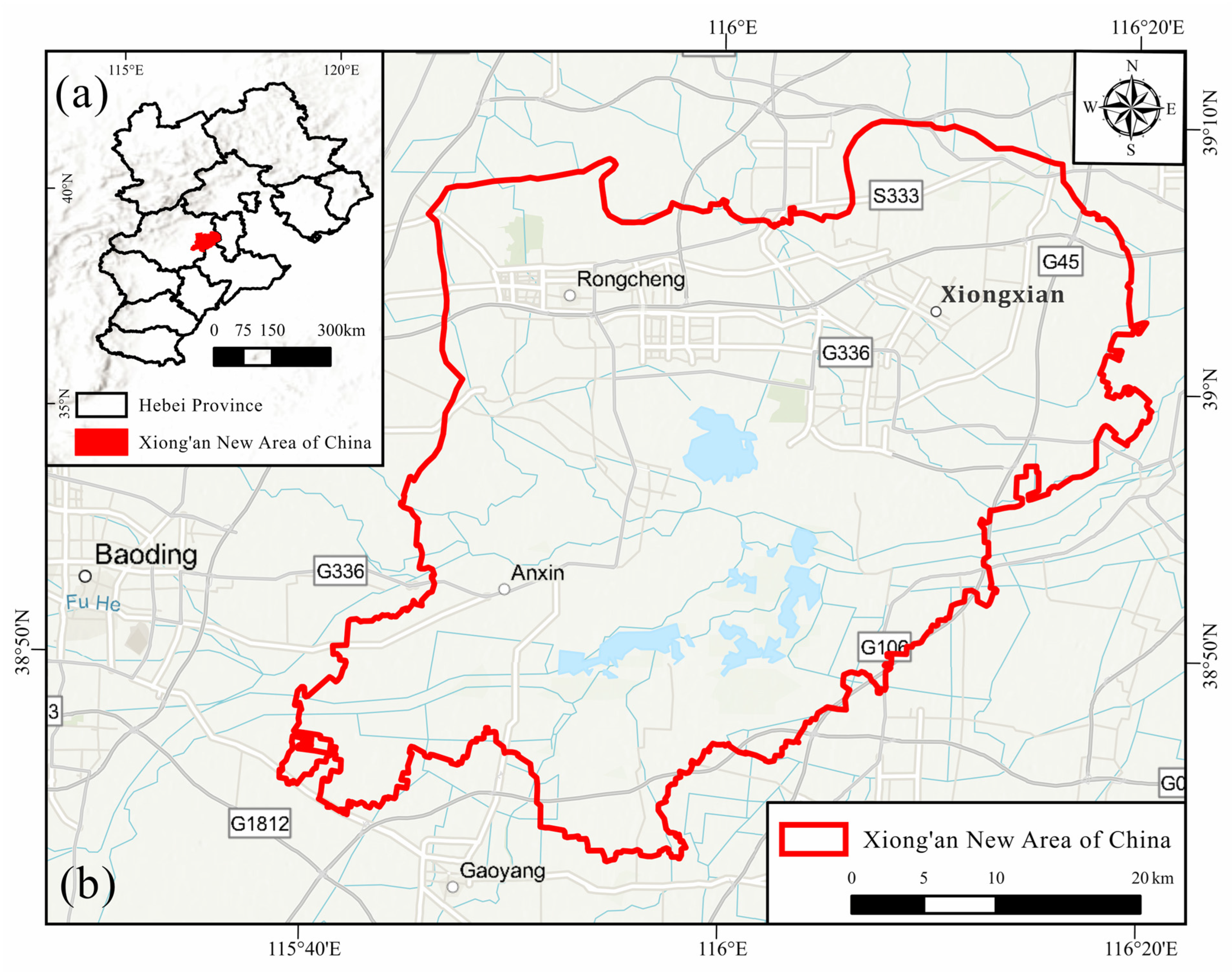
The Xiong’an New Area of China is strategically situated in the heart of Hebei Province, nestled within the confluence of the Beijing, Tianjin, and Hebei regions. The designated area encompasses three counties: Xiongxian, Rongcheng, and Anxin, as well as certain adjoining areas, cumulatively spanning approximately 2000 km2 (refer to Figure 1). Among them, Rongcheng County has the highest population density, followed by Xiong County, and Anxin County has the lowest. This region boasts a myriad of advantageous attributes. Its prime geographic location facilitates convenient transportation routes, and its pristine ecological surroundings underscore a robust capacity for both resource and environmental sustainability. Furthermore, with abundant developmental space available, the foundational groundwork for the Xiong’an New Area is set at both high starting points and exacting standards. Natural water features enhance the landscape of the Xiong’an New Area. The region is laced with rivers such as the Nanjuma River, Daqing River, and Baigou Yin River. It also houses Baiyangdian, the most expansive freshwater lake in the North China Plain. Notably, within the Baiyangdian system, the front edge depression of the alluvial fan of the Daqing River’s tributaries lies within Xiong’an. This depression seamlessly connects the upstream Jiuhe River to the downstream Renhai River, marking the lowest geographical point in the Xiong’an New Area.
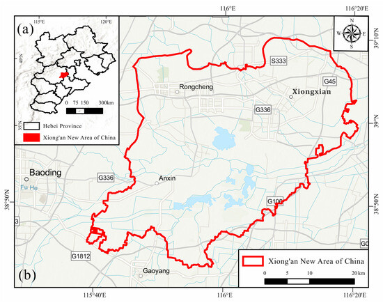
Figure 1.
The geographical location of Xiong’an New Area of China in a large context (a) and Rongcheng, Xiongxian, and Anxin counties within the Xiong’an New Area of China (b).
2.2. Satellite Data
This study utilized 24 remote sensing images spanning six years, from 2016 to 2022, to cover the entire Xiong’an New Area. Out of these images, 20 are from Sentinel-2A, while the remaining 4 are from Sentinel-2B. We specifically chose images taken between July and September, a period when vegetation is at its peak. The details of these images are provided in Table 1.

Table 1.
Sentinel-2A/B images used in this study.
Sentinel-2’s Level-1C data provide apparent reflectance for the upper atmosphere, which has undergone both geometrical and radiometrical corrections. To elevate this to Level-2A data, an atmospheric correction is essential. We used the Sen2Cor software (In 2016 and 2017, the data was collected using version 2.5.5. From 2018 to 2021, version 2.9 was used, and in 2022, version 2.10 was employed), developed by the European Space Agency, to correct atmospheric effects on Sentinel-2 images [22]. Following this, the images were resampled to a 10 m resolution using the ESA’s SNAP9.0 software. Lastly, the ENVI5.3 software facilitated the fusion, mosaicking, and subsetting of the images to produce the final remote sensing products for the Xiong’an New Area.
2.3. Sample Data for Validation
Considering the distribution of different land types in the study area, samples were evenly drawn from each type. Google Earth imagery served as a reference for the selection of validation samples. Taking 2017 as a representative year, we selected a total of 732 validation samples. This comprised 158 samples from construction land, 112 from water bodies, 122 from forests, 110 from cultivated lands, 98 from grasslands, 100 from unused lands, 108 from hydrophytes, and 82 from roads. For the other years under study, each type had between 100 and 200 samples selected.
3. Methodology
3.1. Land Cover Types
In this study, we categorized the land-use types in the Xiong’an New Area into eight distinct categories, as outlined in GB/T 21010-2017: construction land, water, forest, cultivated land, grassland, unused land, hydrophyte, and road [23]. The details of these categories are presented in Table 2.
Table 2.
Land Cover Classification System.
In this context, “construction land” encompasses both urban and rural areas. The “water” category comprises rivers, lakes, ponds, and the like. “Forest” includes both forest land and other types of forests, while “cultivated land” primarily covers paddy fields and dry fields. “Grassland” embraces both artificial and natural grasslands. “Unused land” pertains to undeveloped areas and abandoned farmland. The “hydrophyte” category captures aquatic plant communities such as lotus, reed, water chestnut, and water caltrop, among others. Lastly, “road” spans highways, railways, urban roads, and rural roads, as detailed in Table 2.
3.2. Feature Variables
In our study, we chose the reflectance of eight bands from Sentinel-2 imagery as our primary spectral features. For our analysis, we integrated three vegetation indices: two water indices, and seven red-edge indices [24,25]. We utilized the Gray-Level Co-Occurrence Matrix (GLCM) to extract high-precision texture features. A detailed list of these indices can be found in Table 3. And we devised eight scenarios for the land cover and land-use (LCLU) classifications, as outlined in Table 4.
Table 3.
Description of different feature sets.
Table 4.
The information of experimental scenarios.
3.3. Remote Sensing-Based Ecological Indices
The Tasseled Cap transformation provides an orthogonal transformation of multispectral remote sensing images, focusing on the multidimensional spectral information of elements like soil and vegetation. Post-transformation, the primary components are the Soil Brightness Index (SBI), Greenness Vegetation Index (GVI), and Wetness (WET). These indices, respectively, represent the characteristics of soil, vegetation, and moisture [26]. It is vital to recognize that this transformation is influenced by the unique settings and properties of the sensor being used. As such, transformation coefficients for different sensors are not universally applicable [27]. In our study, the Tasseled Cap parameters specific to Sentinel-2 data are sourced from the Index Database (https://www.indexdatabase.de (accessed on 12 March 2023)) to calculate SBI, GVI, and WET. The computation formula is detailed as follows,
where , , , , , and represent the corresponding band values of Sentinel-2 images, respectively.
The Remote Sensing Based Ecological Index (RSEI) leverages remote sensing data to offer a composite ecological assessment. This index amalgamates various indicators that directly represent the ecological environment, facilitating swift monitoring and evaluation of a region’s ecological state [26]. In our research, we have formulated the RSEI using the comprehensive index method, drawing from the outcomes of the Tasseled Cap transformation. The RSEI is written as
As the RSEI value approaches unity, it indicates an enhancement in ecological quality. Conversely, as the RSEI value deviates further from unity, it signifies a decline in the ecological health of the area.
3.4. Empirical Orthogonal Function (EOF)
To investigate the spatiotemporal variability of the RSEI, this study adopts the EOF model. Initially proposed by Pearson [28] and later introduced into the field of atmospheric science by Lorenz in the 1950s [29], the EOF model has been extensively applied to date [30,31].
EOF analysis is a method for identifying structural characteristics within matrix data and extracting the principal features of the data. EOFs can explain the spatiotemporal variability of variable fields and are known for their stability and fast computational convergence. EOF decomposition is applied to variable fields with spatiotemporal changes. Specifically, it breaks down a series of variable fields, W(x, y, t) n, into a sum of products of mutually orthogonal spatial functions, Vn(x, y, t), and mutually orthogonal temporal functions, Tn(t) [32]
where Cn represents the weighted coefficient.
EOF is used to analyze and process the RSEI, extracting major data features to concentrate information on a few spatial distributions and time series, thus reflecting the spatiotemporal changes of RSEI. Here, the eigenvectors correspond to spatial samples, and the principal components correspond to time coefficients. The differences between the variable fields at different times are due to the different temporal coefficients of each typical field. Different spatial typical fields contribute differently to the overall variable field [33], and analyzing those with significant contributions can highlight the main contradictions in the problem. After EOF decomposition, the spatial distribution of RSEI and the temporal characteristics of this distribution are obtained. When the time coefficient is positive, it indicates that the corresponding spatial distribution is the main form of distribution; the larger the coefficient, the more typical it is. When the time coefficient is negative, it suggests that the current spatial distribution is opposite to the actual situation, and the larger the absolute value of the coefficient, the more apparent the distribution form. High-value areas in the spatial distribution map indicate that these areas are more sensitive and have greater variability.
3.5. Accuracy Assessment
In this study, the accuracy of our classification model was validated using a confusion matrix—a table that juxtaposes predicted results against actual values to assess the level of agreement. Four key evaluation indices were selected: Overall Accuracy (OA), Kappa Coefficient (Kappa), Producer Accuracy (PA), and User Accuracy (UA). The formulas for computing these indices are as follows,
where N represents the total number of samples; k is the total number of types; denotes the sample number correctly classified in the i-th row and i-th column of the error matrix; and and are the numbers of true samples and predicted samples for the i-th type, respectively.
4. Feature Optimization
4.1. Band Combinations
This study uses the Optimum Index Factor (OIF) method to select the best original band combination based on Sentinel-2 remote sensing images [34]. The OIF is defined by
where represents the standard deviation of the i-th band, n represents of the selected band number (usually set to 3), and denotes the correlation coefficient between the i-th and j-th bands. Larger OIF values may have smaller band correlations and better band combinations. The selected optimal indices of band combination and their OIF values for the years 2016–2022 are shown in Table A1.
4.2. Vegetation Indices
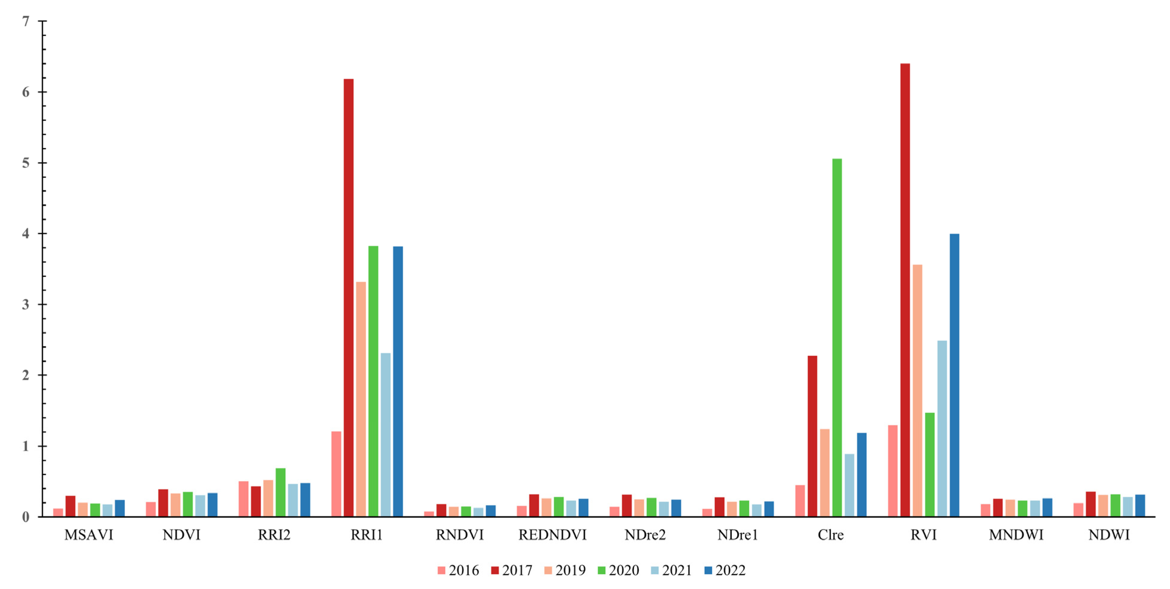
From the acquired imagery, both vegetation indices and red-edge features were extracted and then combined through a layer stacking process. The subsequent standard deviation and correlation matrix were computed and are depicted in Figure A1 and Figure A2, respectively. Notably, the standard deviation measures the dispersion of pixel gray values from their average value in the image; a higher standard deviation signifies a more pronounced dispersion.
Figure A2 graphically presents the feature selection procedure. For the main classification, the features include the following: NDVI, RRI2, NDre1, Clre, and RVI. For the years 2016, 2019, 2021, and 2022, the feature set includes NDVI, RRI2, and RVI. For 2020, the feature set is NDVI, RRI2, and NDre2. This distinction will guide the implementation and evaluation of classification algorithms, ensuring that each year’s classification uses the most relevant feature set. Proper feature selection, as demonstrated, is crucial for achieving higher classification accuracy and making the most out of the available remote sensing data.
4.3. Texture Indices
PCA was applied to the satellite images from each year to identify the most informative textures. The first principal component, which accounted for over 90% of the variance, was chosen for further analysis. Using this component, texture features were derived and their interrelationships are visualized in Figure A2g–l. As indicated in Figure A2h, the correlation among these texture features was generally lower compared with those from the vegetation index and red-edge features. The retained texture features included Mean, Variance, Contrast, Dissimilarity, Second Moment, and Correlation. This selection methodology was consistent across all years, resulting in the aforementioned texture features being chosen every time.
4.4. Water Surface Indices
The water indices derived from the images were combined using a layer stacking approach. Subsequently, the correlation matrix between different bands was computed, with results for the year 2017 presented in Table A2. The standard deviation for these indices is depicted in Figure A1. Taking into account both correlation and standard deviation, NDWI was selected as the representative water index. This selection process was consistent for all years spanning 2016 to 2022, with NDWI being the preferred choice each time.
5. Results
5.1. Land-Use Classification Results Based on Different Feature Combinations
Table 5 presents the classification results across the eight scenarios. When using only spectral features for land surface cover classification in the Xiong’an New Area, the overall accuracy is the lowest, at 94.496%. By incorporating vegetation and water body indices in Scenario 2, the overall accuracy is increased by 0.932%, while the Kappa coefficient experiences a slight rise. Building on Scenario 2, the introduction of red-edge and texture features boosts the overall accuracy and Kappa coefficient by 1.566% and 1.950%, and 0.018 and 0.023 respectively. This underscores that integrating red-edge and texture features can significantly enhance the accuracy of land-use classification in the Xiong’an New Area, with the addition of texture features providing a more noticeable boost compared with the red-edge features. Scenario 5 amalgamates all feature variables and achieves an overall accuracy of 97.382% with a Kappa coefficient of 0.970, though the enhancement is marginal. Out of all of them, Scenario 6 stands out, delivering the highest overall accuracy and Kappa coefficients at 98.673% and 0.984, respectively. Impressively, by paring down the feature variables from 31 to 15, there was an uptick in both accuracy and processing efficiency.
Table 5.
Land-use classification results based on different feature combinations and classifiers in 2017.
The details of the producer’s accuracy and user’s accuracy for each land cover class in scenarios 1–8 are shown in Appendix E.
To assess the effectiveness of the Support Vector Machine (SVM) in land-use classification for the Xiong’an New Area, this study tested three prominent machine learning algorithms: SVM, RF (Random Forests), and NNC (Neural Net Classification), using the optimal band combinations identified post-feature selection. The comparative analysis, as detailed in Table 5, demonstrates that SVM outperforms the other two algorithms. It achieved an impressive overall accuracy of 98.673% and a Kappa coefficient of 0.984. This was 1.412% and 0.016 higher than RF and 0.674% and 0.007 higher than NNC, respectively. In essence, our proposed SVM approach, underpinned by multifaceted feature selection, significantly enhances classification precision in the Xiong’an New Area.
To evaluate the efficacy of the SVM model for land-use classification in the Xiong’an New Area, optimized band combinations were applied to three prevalent machine learning algorithms for remote sensing imagery: Support Vector Machine (SVM), Random Forest (RF), and Neural Net Classification (NNC). These correspond to scenarios 6, 7, and 8, respectively, with the results and processing times presented in Table 5 and Table 6. SVM emerged as the top performer, boasting an overall accuracy of 98.673% and a Kappa coefficient of 0.984. It surpassed RF by 1.412% in accuracy and 0.016 in the Kappa coefficient and outdid NNC by 0.647% in accuracy and 0.007 in the Kappa coefficient. However, its superior performance came at the cost of efficiency, taking 128 min—making it the lengthiest. NNC struck a balance between accuracy and processing speed, ranking second in both. In contrast, while RF offered the quickest classification, it lagged in accuracy. Despite RF’s speed, the limited image dataset in this research shifted the focus to classification precision over processing efficiency. Nonetheless, in larger datasets, the efficiency of RF could be invaluable—despite a marginal drop in accuracy, it cuts processing time by a third, marking it as highly efficient. However, since accuracy was paramount in our study, SVM was selected for subsequent annual classifications.
Table 6.
Classification time for scenarios 6, 7, and 8.
5.2. Land-Use Classification Results Based on Feature Optimization for 2016–2022
Using the optimal spectral features, vegetation indices, red-edge features, and texture features, we applied the SVM algorithm for classification for each year. The classification accuracies spanning from 2016 to 2022 are detailed in Table 7. The overall accuracies for these years were 92.853%, 98.470%, 96.139%, 96.694%, 94.639%, and 95.707%, respectively. Simultaneously, the Kappa coefficients were 0.917, 0.982, 0.953, 0.959, 0.936, and 0.949, respectively. Analyzing the land-use classification results across the years, 2017 boasted the highest accuracy, while 2016 registered the lowest.
Table 7.
Land-use classification results based on feature optimization for 2016–2022.
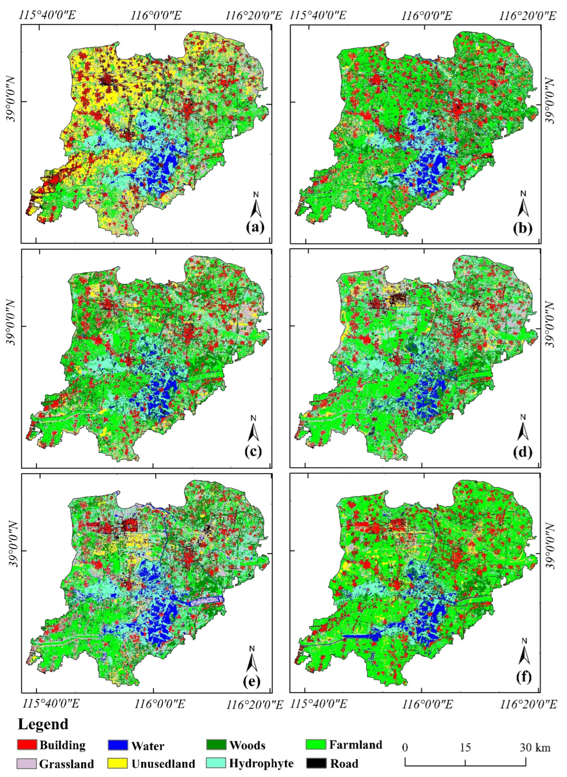
The land-use transition matrix, along with the evolution of land-use patterns in the Xiong’an New Area from 2016 to 2022, is detailed in Table 8 and visualized in Figure 2. The data from these sources highlight that, in 2016, grassland and unused land predominantly characterized the Xiong’an New Area’s landscape. However, by 2022, farmland had emerged as the predominant land-use category, signaling a marked shift from the prior dominance of grassland and unused spaces. The most substantial land conversion was observed in the farmland, which expanded by 518.41 km2. In contrast, water bodies registered the most minimal change, expanding by a mere 9.3 km2. The forested region also saw an augmentation, growing by 68.11 km2, a development attributed substantially to the “Millennium Show Forest” initiative. Conversely, there was a contraction in the extents of grassland, unused land, hydrophytes, and roadways. Of these categories, the grassland experienced the sharpest decline, closely followed by the unused land category.
Table 8.
Land-use transfer matrix from 2016 to 2022.

Figure 2.
Results of feature-based optimization land-use classification images for 2016–2022, 2016 (a), 2017 (b), 2019 (c), 2020 (d), 2021 (e) and 2022 (f).
Between 2016 and 2022, the built-up area expanded from 182.15 km2 to 205.12 km2, predominantly resulting from the conversion of grasslands, unused lands, and roadways. Despite this growth, some buildings were re-purposed into farmland, grasslands, and roads in line with the Xiong’an New Area’s strategic urban planning, which emphasizes a logical layout and the restructuring of infrastructure. Notably, these transformations were most prevalent in the starting area and the northern regions of Rongdong and Rongxi within Rongcheng County. By 2019, settlements in the starting zone had evolved to be denser and more ecologically harmonious. That same year marked the commencement of the Xiong’an Station high-speed railway construction in Jiugang, positioned northeast of Xiongxian County. The year 2020 witnessed the addition of numerous roads and rail links within the starting zone, laying the foundation for an integrated rail transit system linking the Xiong’an New Area both internally and to neighboring urban centers. In 2021, the Baiyangdian water body expanded eastwards and, by 2022, had further grown southwestward, making Baiyangdian a prominent feature across the entire Xiong’an landscape. The “Millennium Show Forest” project, initiated in 2017, has notably bolstered the forest cover in Xiongxian County, counteracting the decline in grassland and unused areas. In terms of developmental vigor, Rongcheng County and Xiongxian County lead the way, while Anxin County lags slightly. Nevertheless, the overarching trajectory for the Xiong’an New Area remains steadfast in its commitment to an environment epitomized by “clear skies, lush lands, and pristine waters”.
5.3. RSEI
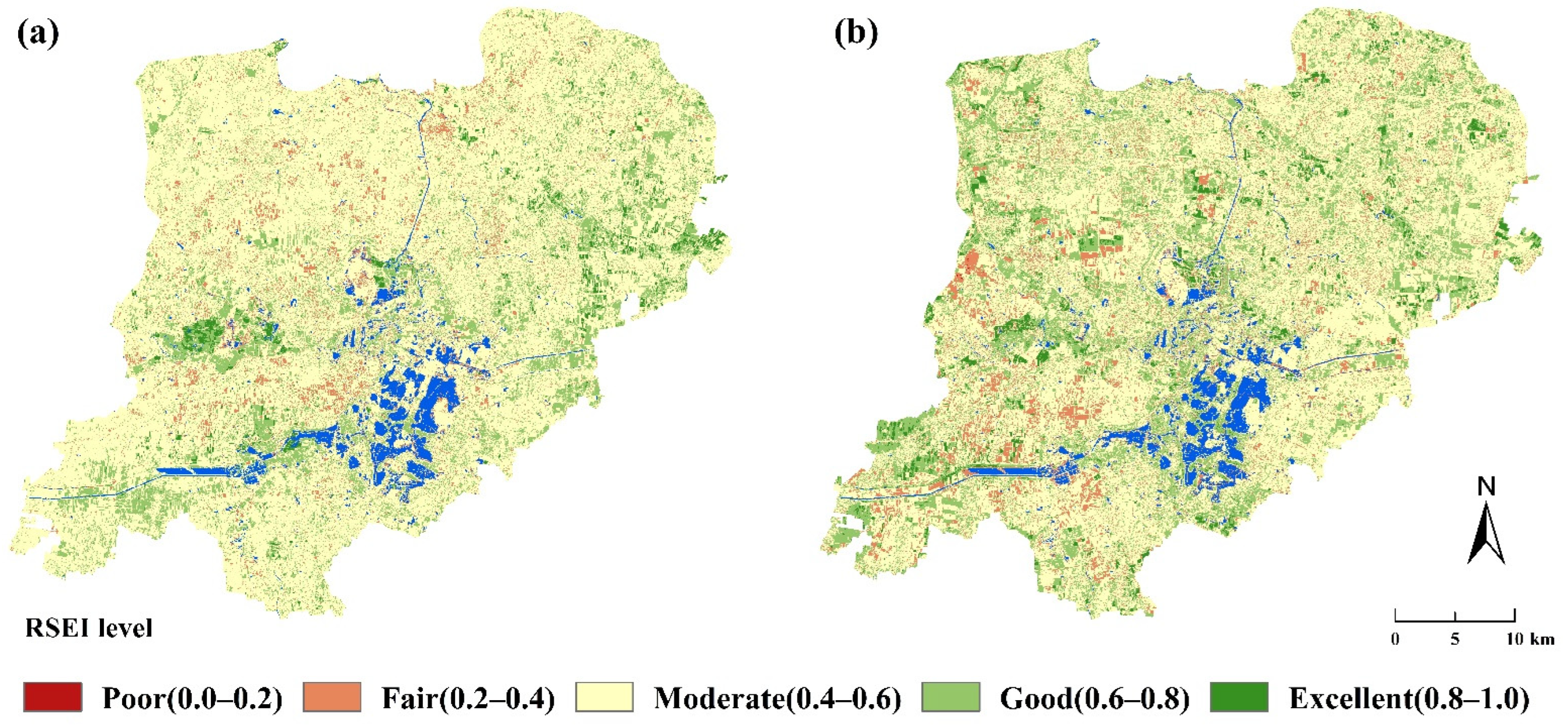
According to Xu [26], the RSEI values are segmented into five distinct levels, each with an interval of 0.2, to depict the spatial distribution of ecological environment quality. These levels are as follows: Level 1: Ecological Inferior (0, 0.2), Level 2: Poor (0.2, 0.4), Level 3: Moderate (0.4, 0.6), Level 4: Good (0.6, 0.8), Level 5: Excellent (0.8, 1). The geographical representation of these RSEI levels can be visualized in Figure 3. Additionally, details such as the area, proportion, and average RSEI value for each level are provided in Table 9.
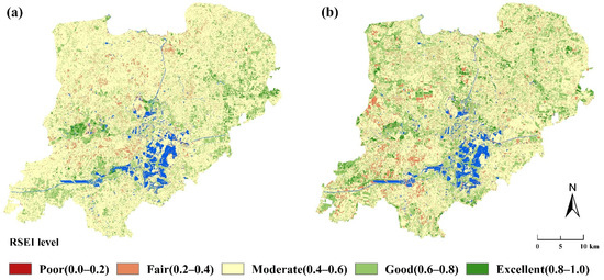
Figure 3.
Leveled-RSEI spatial distribution images of the Xiong’an New Area in 2016 (a) and 2022 (b).
Table 9.
Area and proportion of each RSEI level and RSEI mean of the Xiong’an New Area in 2016 and 2022.
Table 9 indicates that the mean RSEI had been almost unchanged from 2016 to 2022 with only a slight increase of 0.01. In both 2016 and 2022, the predominant RSEI levels in the Xiong’an New Area were ‘Moderate’ and ‘Good’, covering areas of 1573.28 km2 and 1490.34 km2, which correspond to 91.46% and 86.64% of the entire region, respectively. The distribution map of RSEI levels also reveals the expansion of excellent RSEI areas of the Xiong’an New Area in 2022 compared with 2016. In Xiongxian and Anxin Counties, most regions advanced to ‘Good’ and ‘Excellent’ levels, expanding by 142.90 km2 in total. Conversely, areas classified as ‘Poor’ and ‘Fair’ grew by 59.23 km2 across the three counties during this period.
Xiongxian’s overall ecological caliber has seen improvement, largely attributed to the initiation of the “Millennium Forest” initiative. Anxin County, on the other hand, witnessed mixed results, with areas both improving and degrading in ecological quality. Rongcheng County, being the nucleus of the Xiong’an New Area’s development, experienced the most profound development. However, its ecological integrity remained largely unaltered, even showing a slight uptick in certain regions. This stability can be credited to the region’s emphasis on preserving its inherent ecology while incorporating ecological greenways and city parks in its developmental plans.
Land-use maps reveal an augmentation in road networks in 2022 as compared with 2016. However, the Xiong’an New Area’s developmental approach has been holistic, ensuring the inclusion of green belts during road constructions, evident in developments like the urban park belt and the lush environs around the Xiong’an Station Hub. It is noteworthy that as the construction in the Xiong’an New Area is ongoing, some of the ecological projects, especially in Rongcheng County, await completion.
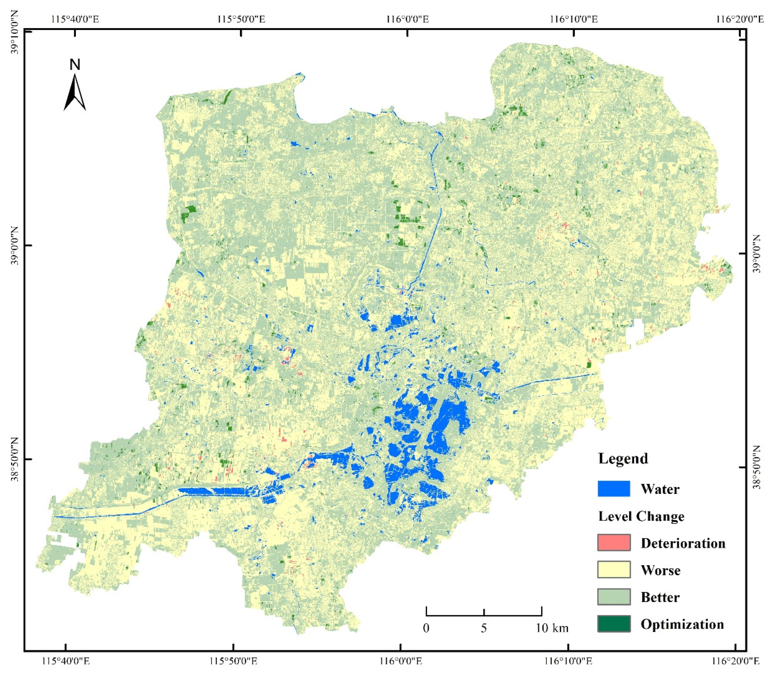
In this study, we also adopted an approach by using a 0.4 interval to categorize the RSEI into four distinct levels. These levels are: ‘Deterioration’ (−0.8 to −0.4), ‘Worse’ (−0.4 to 0), ‘Better’ (0 to 0.4), and ‘Optimization’ (0.4 to 0.8), as proposed by Cai et al. (2020). The spatial variations in these RSEI levels are visually depicted in Figure 4.
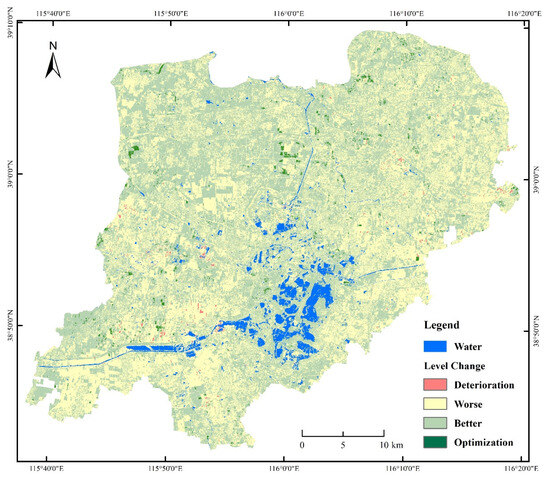
Figure 4.
Changes in RSEI levels in the Xiong’an New Area between 2016 and 2022.
Figure 4 and Table 10 reveal that between 2016 and 2022, 48.57% of the areas witnessed a deterioration in ecological quality. In contrast, 51.43% exhibited improvements, with a spread of 2.86% favoring the latter. Notably, areas with marginal alterations (categorized as ‘Worse’ and ‘Better’) made up 98.62% of the total. Those undergoing significant positive (Optimization) or negative (Deterioration) shifts accounted for only 1.38%. The majority of improved regions were found in Rongcheng and Xiongxian counties, whereas most of the deteriorating areas lay within Anxin County. Land-use classification maps suggest that Rongcheng and Xiongxian counties had experienced a more intense developmental phase compared with Anxin County. As the Xiong’an New Area’s development strategy underscores the importance of ecological preservation, the evident RSEI level enhancement in Rongcheng and Xiongxian signifies the effective ecological management integrated into their development. Conversely, the predominant focus on cropping in Anxin County, combined with the impact of seasonal weather on immature crops, contributed to the observed decline in its ecological standing. On the whole, the ecological trajectory of the development of the Xiong’an New Area leans positively, mirroring its commitment to prioritizing ecology and promoting sustainable development.
Table 10.
Area and proportion of RSEI level change in the Xiong’an New Area between 2016 and 2022.
5.4. The Spatiotemporal Distribution Characteristics of RSEI
To analyze the spatiotemporal characteristics of the RSEI on the interannual scale in the Xiong’an New Area, an EOF decomposition was performed on the RSEI indices calculated from remote sensing images from 2016 to 2022. The temporal mean values are removed from the original RSEI at every spatial location to ensure that both the spatial mode and temporal mode reflect the RSEI variability.
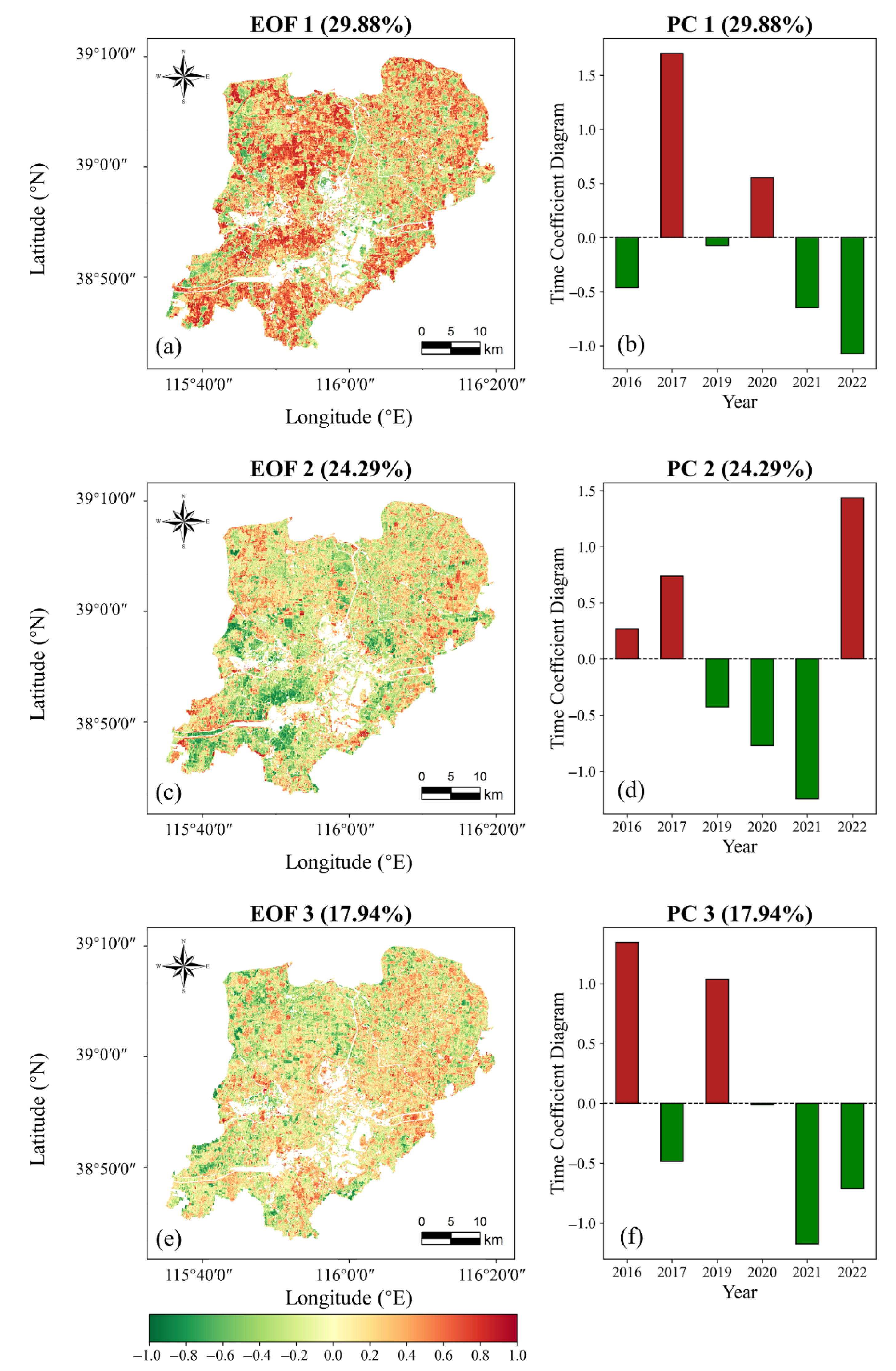
Figure 5a,c,e present the first, second, and third spatial modes obtained from the EOF decomposition. Figure 5b,d,f depict the temporal modes of the EOFs. The variance contribution rates of the modes are 29.88%, 24.29%, and 17.94%, respectively, with a cumulative contribution rate reaching 72.11%, indicating that the first three modes can describe the majority of the RSEI variations.
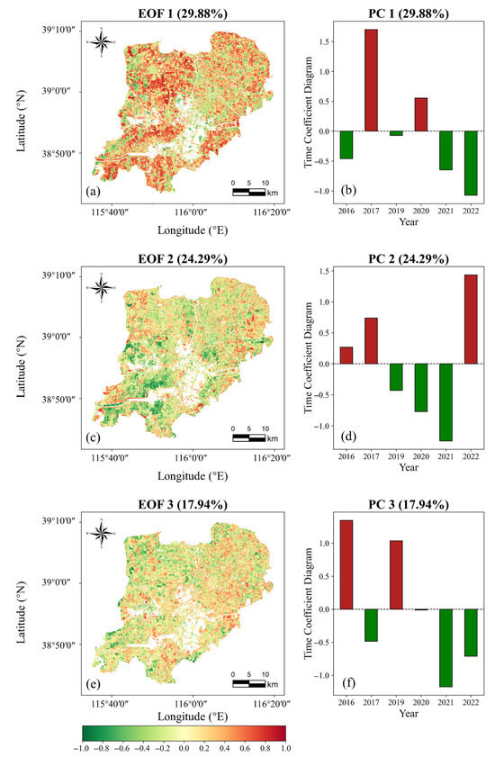
Figure 5.
EOF analyses of RSEI in Xiong’an New Area from 2016 to 2022 with the first spatial mode (a) and temporal mode (b), the second spatial mode (c) and temporal mode (d), and the third spatial mode (e) and temporal mode (f).
The first mode of EOF (EOF1) illustrates a typical spatial distribution pattern of RSEI in the Xiong’an New Area. Generally, the west side of the region, specifically in Anxin and Rongcheng counties, exhibits positive values, whereas the Xiongxian area on the east side displays negative values in the first spatial mode (Figure 5a). The first temporal mode (Figure 5b) fluctuates between positive and negative values, starting from 2017. When combining the features of both the first spatial and temporal modes, it becomes evident that the RSEI has been in a continuous decline since 2017 in Anxin and Rongcheng. In contrast, the eastern side in Xiongxian has seen an upward trend in RSEI since 2017, as indicated by the negative values in the first spatial mode.
The second mode, shorter in temporal variation compared with the first, reflects the impact of transient driving forces (Figure 5c). Its spatial mode (Figure 5c) shows negative values predominantly on the southern side, mainly in Anxin county, while positive values are more common in Rongcheng and Xiongxian. Starting from 2017, the second temporal mode has shown a decline from a positive value to a negative value (Figure 5d). This suggests that areas with negative values in the spatial mode have experienced increasing RSEI values, although there was a sharp decrease in 2023. For Xiongxian and Rongcheng, significant improvements in RSEI are projected for 2023, likely influenced by transient processes, including climate variations and anthropogenic factors like urban expansion and ecological restoration initiatives in the development of the Xiong’an New Area.
The third spatial mode reveals a mixed distribution of positive and negative anomalies (Figure 5e). Although lacking distinct centers of high or low values, the positive anomalies are primarily scattered towards the eastern parts of the Xiong’an New Area, while negative anomalies are mostly found in the northwest, showing an inverse distribution pattern. The temporal mode fluctuates approximately every two years, as shown in Figure 5f. In 2016 and 2017, the temporal mode was positive, indicating an increase in RSEI in the northwest and a decrease in the east. Conversely, in 2021 and 2023, a negative temporal mode suggests a decrease in RSEI in the northwest and an increase in the east.
6. Discussion
In our study, a variety of feature vectors were derived from the images by employing the technique of computing feature indices. To identify the most pertinent features, we utilized selection methodologies including the OIF index, correlation analysis, standard deviation assessment, and principal component analysis. The comparative analysis of outcomes, both with varying feature additions and those based on the optimized features, can be seen in Table A1 and Table A2, as well as in Figure A1 and Figure A2. The corresponding classification outcomes are detailed in Table 5.
Single spectral feature-based scenarios yield satisfactory accuracy, making them suitable for studies with moderate classification precision needs. However, when integrating multiple feature variables, the accuracy noticeably improves. Notably, the scheme that leverages feature selection attains the highest accuracy. Concerning land cover classifications, adding texture features bolsters the accuracy for structures and forests. Water classifications remain consistently high across all schemes. Both texture and red-edge features play pivotal roles in enhancing the producer’s accuracy for hydrophytes. As for road classifications, the influence of red-edge and texture features far outweighs that of vegetation and water indices.
In the realm of land-use classification, an ever-growing body of scholars is turning to feature selection methods. Studies conducted in diverse regions like the Southern Hilly Region and Cultivated Areas have deployed these techniques, typically focusing on less developed areas predominated by vegetation and crops [4]. Our study area contrasts with these regions, encompassing a blend of urban and rural landscapes, a well-structured transportation system, and Baiyangdian, the largest freshwater wetland in the North China Plain. This diverse array of land cover types introduces more complexities into land-use classification. For instance, Li et al. [4] included six features but omitted texture features, a crucial aspect of land-use classification. We have advanced beyond the scope of Li et al.’s research, consciously excluding radar and terrain features due to our study area’s flat plain topography, where terrain effects are negligible. We reached this decision after finding, in line with Li et al.’s results, that the inclusion of radar features would diminish the accuracy in classifying building areas and unused land. Therefore, our approach offers a more tailored method for the specific challenges and characteristics of our study area.
Historically, land-use classification studies on the Xiong’an New Area have predominantly hinged on conventional methods, either spectral feature-centric (as demonstrated by Yu et al. [11]) or employing object-oriented paradigms (like Jia et al. [12]). Diverging from this trend, our approach hinges on an innovative feature selection method. This methodology amalgamates a diverse array of features—spectral, textural, water indices, and red-edge features—selecting the most pivotal ones to ensure succinctness, thus circumventing data redundancy. Furthermore, while prior research typically compartmentalized the area’s land use into 5–6 categories, our study meticulously subdivided it into eight distinct classes, enhancing granularity. Our method catapulted classification accuracy, achieving an unprecedented 98.673%, a marginal improvement even over previous work [11].
The land-use changes observed between 2016 and 2022 in the Xiong’an New Area demonstrate a pronounced transformation in the regional landscape. Most prominently, the marked decrease in unused land and grasslands suggests that these areas have likely been repurposed for other land-use categories. Marginal reductions in the area occupied by aquatic plants and roads further underscore the dynamic nature of this region’s development. Conversely, the uptick in building, water body, and forest areas provides evidence of urban expansion, conservation efforts, or both.
However, it is the dramatic proliferation of farmland that stands out most conspicuously. Almost doubling its footprint since 2016, this surge in farmland challenges conventional expectations. Such a pronounced increase in agricultural territory within a relatively short time frame is atypical, especially in an era where urban expansion often encroaches upon arable land.
Upon scrutinizing the satellite imagery from both 2016 and 2022, distinct phenological differences in crop stages become evident. The 2016 image, captured on 30 September, depicts the region during a period when predominant crops, including rice and summer corn, had attained their maturity and were on the cusp of harvest. Conversely, the 2022 image, dated 21 July, captures a moment within the vegetative phase of the crop cycle when plants are vigorously growing and exhibiting maximal canopy coverage. This difference in growth stages leads to an optical illusion in satellite-derived land-use data, suggesting an expanded farmland expanse in the 2022 imagery. The crops’ denser foliage during their vegetative phase contributes to this perceived enlargement, compared with the more subdued appearance of crops nearing harvest in the 2016 image. Furthermore, this study solely focuses on the correlation between the vegetation index and red-edge characteristics, neglecting the potential high correlation among four key features: the vegetation index, red-edge characteristics, texture features, and water body index. Future research could benefit from an in-depth exploration of the interrelationships among these attributes.
An exploration into the ecological quality change in the Xiong’an New Area between 2017 and 2020, utilizing Landsat data [11], shed light on the non-declining, slightly improving ecological state during this period. Such positive alterations, where areas witnessing ecological progress clearly outpaced degraded zones, paved the foundation for our comparative analysis. This study delved deeper, juxtaposing the ecological standards of the Xiong’an New Area prior to its 2016 inception with the data up to 2022. It illuminated a consistent upward trajectory, with enhanced ecological conditions. This research finding is observable in the land-use classification results. Interestingly, these revelations bolster the argument that the Xiong’an New Area’s urban planning has steadfastly been eco-centric, embracing sustainable development principles. This strategic approach has, commendably, shielded the region from the ecological deterioration often accompanying rampant urbanization.
Although RSEI is one of the most widely used comprehensive evaluation indices for ecological environment quality, Wang et al. [35] have pointed out that this index, being entirely based on remote sensing data, has limitations in its application. For example, its calculation process cannot consider all ecological elements (especially water elements). Despite its wide application, there have been few improvements to RSEI’s limitations. Therefore, Wang and others have improved RSEI, and the results show that the improved model aligns more closely with the real ecological environment. This study will refer to Wang and others’ improved model in subsequent research to more accurately reveal the ecological environment quality of the Xiong’an New Area.
Since its establishment in 2017, the Xiong’an New Area, as a national-level new area, has undergone a rapid urbanization process. Rapid urbanization usually leads to a singular transformation in land-use types, with most land being converted to construction sites and roads, and causes many ecological and environmental problems. However, this trend is not evident in the Xiong’an New Area. In the land-use types of Xiong’an, construction land, water bodies, forest land, and arable land have all increased. Also, as indicated by the RSEI results, the ecological environment has not deteriorated. The Xiong’an New Area will serve as a new model for high-quality development in a new era. This suggests that the impact of rapid urbanization on land use and urban ecology in the future will be different from the past, leading to new understandings of urbanization.
Peering into the future, machine learning’s triumphant run in delivering top-notch classification accuracy prompts a logical progression towards deep learning techniques. These techniques, with their innate ability to autonomously discern and employ optimal features for classifications, can revolutionize accuracy levels. A compelling area of exploration would be to juxtapose the innate automatic feature discernment capabilities of deep learning against traditional machine learning’s feature selection to discern the superior technique for the Xiong’an New Area’s land-use classification.
7. Conclusions
This research undertook the meticulous task of evaluating land-use patterns in the Xiong’an New Area, harnessing a comprehensive assortment of features–spectral indices, vegetation indices, water indices, red-edge features, and texture features. A total of eight unique scenarios were devised, merging various feature variables, with the classification capabilities of three machine learning methodologies—Support Vector Machines (SVM), Random Forest (RF), and Neural Network Classifier (NNC)—put to the test. The key findings are summarized as follows:
- (1)
- Adding spectral features along with other variables can enhance the classification capability of different land cover types. By conducting feature selection, the number of feature variables is reduced from 31 to 15. Combining the results of feature selection with an SVM (Support Vector Machine) classifier achieves the best classification results, with an overall accuracy of 98.673% and a kappa coefficient of 0.984.
- (2)
- Based on the classification results from 2016 and 2022, as well as the spatial distribution of RSEI (Remote Sensing Ecological Index), it can be observed that the ecological quality in 2022 has improved compared with 2016. Moreover, both the development trend and RSEI level of Rongcheng County and Xiongxian County are better than those of Anxin County.
- (3)
- The EOF analyses clearly reveal a division in ecological conditions, with positive RSEI values in the western regions (Anxin and Rongcheng) and negative values in the east (Xiongxian), coupled with a fluctuating temporal mode indicating a decline in the west and an increase in the east since 2017. The RSEI has undergone short-cycle fluctuations, underscoring the area’s dynamic ecological state, which highlights the area’s dynamic ecological state, shaped by both long-term trends and transient factors.
The meticulous approach adopted in this study and the resultant findings promise to be instrumental in guiding future developmental and ecological endeavors within the Xiong’an New Area.
Author Contributions
Conceptualization, Q.O. and J.P.; methodology, Q.O. and J.P.; software, Q.O.; validation, Q.O.; formal analysis, Q.O. and J.P.; investigation, Q.O. and J.P.; resources, J.P.; data curation, Q.O.; writing—original draft preparation, Q.O.; writing—review and editing, J.P.; visualization, Q.O. and J.P.; supervision, J.P.; project administration, J.P.; funding acquisition, J.P. All authors have read and agreed to the published version of the manuscript.
Funding
This study is supported by National Key R&D Program of China grant # 2021YFB3900400.
Data Availability Statement
Data are contained within the article.
Conflicts of Interest
The authors declare no conflicts of interest.
Appendix A
Table A1.
Optimal indices of band combination in 2016–2022.
Table A1.
Optimal indices of band combination in 2016–2022.
| Year | Optimum Index Factor | Group |
|---|---|---|
| 2016 | 0.129 | Band 8, Band 8A, Band 12 |
| 2017 | 0.231 | Band 4, Band 7, Band 8A |
| 2019 | 0.151 | Band 4, Band 8A, Band 9 |
| 2020 | 0.169 | Band 4, Band 8A, Band 9 |
| 2021 | 0.138 | Band 4, Band 8A, Band 9 |
| 2022 | 0.191 | Band 4, Band 8A, Band 9 |
Appendix B

Figure A1.
Standard deviation of vegetation indices and red-edge features for 2016–2022.
Figure A1.
Standard deviation of vegetation indices and red-edge features for 2016–2022.
Appendix C
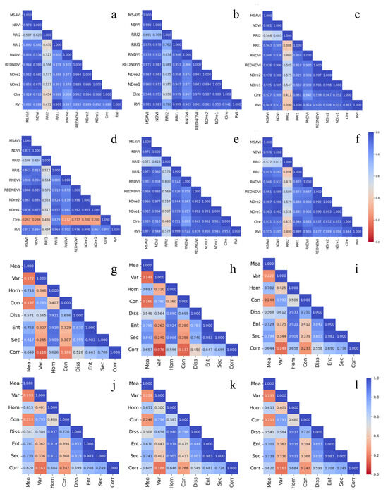
Figure A2.
The correlation coefficient matrix of vegetation indices and red-edge features for 2016–2022 ((a–f), respectively), and the correlation coefficient matrix of texture indices for 2016–2022 ((g–l), respectively).
Figure A2.
The correlation coefficient matrix of vegetation indices and red-edge features for 2016–2022 ((a–f), respectively), and the correlation coefficient matrix of texture indices for 2016–2022 ((g–l), respectively).

Appendix D
Table A2.
Water indices correlation for 2016–2022.
Table A2.
Water indices correlation for 2016–2022.
| Year | Correlation | MNDWI | NDWI |
|---|---|---|---|
| 2016 | MNDWI | 1.000 | 0.868 |
| NDWI | 0.868 | 1.000 | |
| 2017 | MNDWI | 1.000 | 0.978 |
| NDWI | 0.978 | 1.000 | |
| 2019 | MNDWI | 1.000 | 0.966 |
| NDWI | 0.966 | 1.000 | |
| 2020 | MNDWI | 1.000 | 0.967 |
| NDWI | 0.967 | 1.000 | |
| 2021 | MNDWI | 1.000 | 0.911 |
| NDWI | 0.911 | 1.000 | |
| 2022 | MNDWI | 1.000 | 0.966 |
| NDWI | 0.966 | 1.000 |
Appendix E
Table A3, Table A4 and Table A5 display the intricate classification outcomes for each scheme, breaking down both the producer’s and user’s accuracy. When analyzing the outcomes across different schemes, it becomes evident that texture features play a pivotal role in bolstering the accuracy of building classifications, particularly when juxtaposed with vegetation indices, water indices, and red-edge features. Introducing a water index notably elevates the producer’s accuracy for water, yet the influence of vegetation indices, red-edge features, and texture features on water classification remains minimal. In the context of forestland, employing vegetation indices and water indices provides a notable uptick in producer’s accuracy by 2.34%, when compared with merely using spectral features. Although red-edge features outshine texture features in amplifying the producer’s accuracy for forestland, the amalgamation of both texture and red-edge features considerably augments the user’s accuracy for this category. For hydrophyte, the incorporation of vegetation indices and water indices offers a marked improvement in user’s accuracy over solely spectral-based classifications. Introducing either texture or red-edge features further boosts the producer’s accuracy, with texture features standing out by escalating the producer’s accuracy by a remarkable 9.21%. However, a convergence of all features appears to diminish the producer’s accuracy. Notably, the most optimal classification outcomes emerge post feature-variable optimization. Lastly, when observing roads, it is evident that red-edge and texture features leave a more pronounced impact compared with vegetation indices and water indices.
From Table A4 and Table A5, it is evident that all three classifiers—SVM, RF, and NNC—demonstrated a high producer’s accuracy and user’s accuracy for water. As observed in scenario 1 from Table A3, using only spectral information for water classification yielded a commendable user’s accuracy of 98.2%. This underscores the imagery’s capability to distinctly discern water from other land cover types. When it comes to green land cover categories like vegetation and croplands, SVM clearly surpassed both RF and NNC in terms of accuracy, with RF trailing as the least accurate. Conversely, for the classification of roads, RF excelled in accuracy, while NNC lagged behind, securing the lowest accuracy.
Our analysis revealed that while the inclusion of specific features can enhance classification accuracy, simultaneously incorporating all features might compromise accuracy for certain land cover categories. Specifically, forest, grassland, unused land, hydrophyte, and roads exhibited a decline in their producer’s accuracy. Concurrently, the user’s accuracy for categories such as buildings, water, forest, farmland, and unused land also deteriorated when all the features were assimilated. This trend underscores a critical observation: while multifaceted feature inputs enrich the dataset with more information, they also introduce the potential for irrelevant and redundant data, which in turn can adversely affect classification precision.
Table A3.
The producer’s accuracy and user’s accuracy for each land cover class in scenarios 1 to 3.
Table A3.
The producer’s accuracy and user’s accuracy for each land cover class in scenarios 1 to 3.
| Scenario 1 | Scenario 2 | Scenario 3 | ||||
|---|---|---|---|---|---|---|
| Producer’s Accuracy | User’s Accuracy | Producer’s Accuracy | User’s Accuracy | Producer’s Accuracy | User’s Accuracy | |
| Building | 95.40 | 97.46 | 95.91 | 93.50 | 95.13 | 97.64 |
| Water | 95.61 | 98.20 | 98.39 | 98.80 | 98.97 | 98.52 |
| Woods | 92.94 | 86.86 | 95.26 | 84.26 | 96.29 | 91.79 |
| Farmland | 95.77 | 95.06 | 97.47 | 97.19 | 98.53 | 96.86 |
| Grassland | 95.63 | 95.53 | 98.75 | 95.43 | 98.34 | 96.92 |
| Unused land | 98.56 | 98.91 | 96.25 | 98.67 | 98.98 | 98.98 |
| Hydrophyte | 87.24 | 89.11 | 86.83 | 98.78 | 91.30 | 98.03 |
| Road | 94.56 | 96.52 | 94.97 | 95.46 | 97.23 | 97.19 |
Table A4.
The producer’s accuracy and user’s accuracy for each land cover class in scenarios 4 to 6.
Table A4.
The producer’s accuracy and user’s accuracy for each land cover class in scenarios 4 to 6.
| Scenario 4 | Scenario 5 | Scenario 6 | ||||
|---|---|---|---|---|---|---|
| Producer’s Accuracy | User’s Accuracy | Producer’s Accuracy | User’s Accuracy | Producer’s Accuracy | User’s Accuracy | |
| Building | 96.37 | 98.54 | 96.05 | 98.49 | 96.32 | 99.95 |
| Water | 99.11 | 98.97 | 99.69 | 98.69 | 99.76 | 98.28 |
| Woods | 95.65 | 96.19 | 94.53 | 94.83 | 99.53 | 95.89 |
| Farmland | 96.82 | 97.02 | 99.33 | 96.46 | 97.30 | 99.89 |
| Grassland | 98.44 | 95.56 | 97.09 | 97.39 | 99.65 | 99.15 |
| Unused land | 99.17 | 99.12 | 98.66 | 98.82 | 98.29 | 98.07 |
| Hydrophyte | 96.04 | 96.59 | 94.36 | 98.06 | 98.52 | 97.62 |
| Road | 97.33 | 95.74 | 96.91 | 96.47 | 97.35 | 98.32 |
Table A5.
The producer’s accuracy and user’s accuracy for each land cover class in scenarios 7 and 8.
Table A5.
The producer’s accuracy and user’s accuracy for each land cover class in scenarios 7 and 8.
| Scenario 7 | Scenario 8 | |||
|---|---|---|---|---|
| Producer’s Accuracy | User’s Accuracy | Producer’s Accuracy | User’s Accuracy | |
| Building | 97.43 | 92.01 | 97.75 | 99.95 |
| Water | 99.62 | 99.21 | 99.74 | 98.98 |
| Woods | 99.55 | 94.34 | 99.64 | 94.47 |
| Farmland | 95.07 | 99.96 | 96.56 | 99.75 |
| Grassland | 93.89 | 99.56 | 99.37 | 99.17 |
| Unused land | 97.86 | 96.38 | 98.70 | 95.62 |
| Hydrophyte | 98.89 | 93.75 | 97.10 | 99.57 |
| Road | 98.86 | 98.34 | 92.72 | 96.43 |
References
- Wu, S.S.; Qiu, X.M.; Usery, E.L.; Wang, L. Using geometrical, textural, and contextual information of land parcels for classification of detailed urban land use. Ann. Assoc. Am. Geogr. 2009, 99, 76–98. [Google Scholar] [CrossRef]
- Kitada, K.; Fukuyama, K. Land-use and land-cover mapping using a gradable classification method. Remote Sens. 2012, 4, 1544–1558. [Google Scholar] [CrossRef]
- Qi, C.M.; Wang, Y.P.; Tian, W.J.; Wang, Q. Multiple kernel boosting framework based on information measure for classification. Chaos Solitons Fractals 2016, 89, 175–186. [Google Scholar] [CrossRef]
- Chen, T.Y.; Yang, C.B.; Han, L.G.; Guo, S.M. GF-2 Data for Lithological Classification Using Texture Features and PCA/ICA Methods in Jixi, Heilongjiang, China. Remote Sens. 2023, 15, 4676. [Google Scholar] [CrossRef]
- Palanisamy, P.A.; Jain, K.; Bonafoni, S. Machine Learning Classifier Evaluation for Different Input Combinations: A Case Study with Landsat 9 and Sentinel-2 Data. Remote Sens. 2023, 15, 3241. [Google Scholar] [CrossRef]
- Li, Y.; Yuan, H.; Luo, J.S.; Liu, Y.; Gou, K. Study on the Evaluation of Ecological Environment Quality Based on RSEI Model. Geomat. Spat. Inf. Technol. 2021, 44, 117–119+124. [Google Scholar]
- Paul, S.S.; Li, J.; Wheate, R.; Li, Y. Application of object oriented image classification and Markov chain modeling for land use and land cover change analysis. J. Environ. Inform. 2018, 31, 30–40. [Google Scholar] [CrossRef]
- Li, H.; Gu, H.; Han, Y.; Yang, J. Object-oriented classification of high-resolution remote sensing imagery based on an improved colour structure code and a support vector machine. Int. J. Remote Sens. 2010, 31, 1453–1470. [Google Scholar] [CrossRef]
- Zou, Y.H.; Zhao, W.X. Making a new area in Xiong’an: Incentives and challenges of China’s“Millennium Plan”. Geoforum 2018, 88, 45–48. [Google Scholar] [CrossRef]
- Deng, W.H.; Wen, X.L.; Xu, H.Q.; Duan, W.F.; Li, C.Q. Analysis of regional development and its ecological effects: A case study of Xiong’an New Area, China. Acta Ecol. Sin. 2023, 43, 263–273. [Google Scholar]
- Yu, M.; Ma, H.B.; Wang, H.W. Analysis of land use change in Xiong’an New Area from 2016 to 2019 based on the Sentinel-2 images. Bull. Surv. Mapp. 2021, 537, 6. [Google Scholar]
- Jia, Y.N.; Zhang, W.C.; Kang, H.T.; Bai, Y.; Bao, J.P. Research on land cover change of Xiong’an New Area from 2016 to 2019. Bull. Surv. Mapp. 2020, 522, 76–79. [Google Scholar]
- Xu, H.Q.; Shi, T.T.; Wang, M.Y.; Fang, C.Y.; Lin, Z.L. Predicting effect of forthcoming population growth–induced impervious surface increase on regional thermal environment: Xiong’an New Area, North China. Build. Environ. 2018, 136, 98–106. [Google Scholar] [CrossRef]
- Xu, B.Q. China’s National New Areas in the ecological transition. Environ. Dev. Sustain. 2023, 25, 3747–3770. [Google Scholar] [CrossRef]
- Xu, H.Q.; Wang, M.Y.; Shi, T.T.; Guan, H.D.; Fang, C.Y.; Lin, Z.L. Prediction of ecological effects of potential population and impervious surface increases using a remote sensing based ecological index (RSEI). Ecol. Indic. 2018, 93, 730–740. [Google Scholar] [CrossRef]
- Luo, J.S.; Ma, X.W.; Chu, Q.F.; Xie, M.; Cao, Y.J. Characterizing the up-to-date land-use and land-cover change in Xiong’an New Area from 2017 to 2020 using the multi-temporal sentinel-2 images on Google Earth Engine. ISPRS Int. J. Geo-Inf. 2021, 10, 464. [Google Scholar] [CrossRef]
- Huo, J.G.; Shi, Z.Q.; Zhu, W.B.; Xue, H.; Chen, X. A Multi-Scenario Simulation and Optimization of Land Use with a Markov–FLUS Coupling Model: A Case Study in Xiong’an New Area, China. Sustainability 2022, 14, 2425. [Google Scholar] [CrossRef]
- Wang, Z.Y.; Cao, J.S. Assessing and Predicting the Impact of Multi-Scenario Land Use Changes on the Ecosystem Service Value: A Case Study in the Upstream of Xiong’an New Area, China. Sustainability 2021, 13, 704. [Google Scholar] [CrossRef]
- Li, Y.; Lu, C.P.; Liu, G.; Chen, Y.; Zhang, Y.; Wu, C.C.; Liu, B.; Shu, L.C. Risk assessment of wetland degradation in the Xiong’an New Area based on AHP-EWM-ICT method. Ecol. Indic 2023, 153, 110443. [Google Scholar] [CrossRef]
- Wu, C.H.; Wang, M.; Wang, C.; Zhao, X.; Liu, Y.J.; Masoudi, A.; Yu, Z.J.; Liu, J.Z. Reed biochar improved the soil functioning and bacterial interactions: A bagging experiment using the plantation forest soil (Fraxinus chinensis) in the Xiong’an new area, China. J. Clean. Prod. 2023, 410, 137316. [Google Scholar] [CrossRef]
- Yang, M.; Gong, J.; Zhao, Y.; Wang, H.; Zhao, C.P.; Yang, Q.; Yin, Y.; Wang, Y.; Tian, B. Landscape Pattern Evolution Processes of Wetlands and Their Driving Factors in the Xiong’an New Area of China. Int. J. Environ. Res. Public Health 2021, 18, 4403. [Google Scholar] [CrossRef] [PubMed]
- Louis, J.; Pflug, B.; Main-Knorn, M.; Debaecker, V.; Mueller-Wilm, U.; Iannone, R.Q.; Cadau, E.G.; Cadau, V.; Gascon, F. Sentinel-2 global surface reflectance level-2A product generated with Sen2Cor. In Proceedings of the IGARSS 2019-2019 IEEE International Geoscience and Remote Sensing Symposium, Yokohama, Japan, 28 July–2 August 2019; pp. 8522–8525. [Google Scholar]
- GB/T 21010-2017; Land-Use Status Classification. General Administration of Quality Supervision, Inspection and Quarantine of the People’s Republic of China, China National Standardization Management Committee: Beijing, China, 2017.
- Michael, J.H. Vegetation index suites as indicators of vegetation state in grassland and savanna: An analysis with simulated SENTINEL 2 data for a North American transect. Remote Sens. Environ. 2013, 137, 94–111. [Google Scholar]
- Shang, J.L.; Liu, J.G.; Ma, B.L.; Zhao, T.; Jiao, X.F.; Geng, X.Y.; Huffman, T.; Kovacs, J.M.; Walters, D. Mapping spatial variability of crop growth conditions using RapidEye data in Northern Ontario, Canada. Remote Sens. Environ. 2015, 168, 113–125. [Google Scholar] [CrossRef]
- Xu, H.Q. A Remote Sensing Urban Ecological Index and its Application. Acta Ecol. Sin. 2013, 33, 7853–7862. [Google Scholar]
- Liu, Q.S.; Liu, G.H.; Huang, C.; Xie, C.H. Comparison of Tasseled Cap transformations based on the selective bands of Landsat 8 OLI TOA reflectance images. Int. J. Remote Sens. 2015, 36, 417–441. [Google Scholar] [CrossRef]
- Pearson, K. On lines and planes of closest fit to systems of points in space. Lond. Edinb. Dublin Philos. Mag. J. Sci. 1901, 2, 559–572. [Google Scholar] [CrossRef]
- Lorenz, E.N. Empirical Orthogonal Functions and Statistical Weather Prediction; Massachusetts Institute of Technology, Department of Meteorology: Cambridge, UK, 1956; Volume 1, p. 52. [Google Scholar]
- Miller, J.K.; Dean, R.G. Shoreline variability via empirical orthogonal function analysis: Part II relationship to nearshore conditions. Coast. Eng. 2007, 54, 133–150. [Google Scholar] [CrossRef]
- Thorson, J.T.; Cheng, W.; Hermann, A.J.; Ianelli, J.N.; Litzow, M.A.; O’Leary, C.A.; Thompson, G.G. Empirical orthogonal function regression: Linking population biology to spatial varying environmental conditions using climate projections. Glob. Chang. Biol. 2020, 26, 4638–4649. [Google Scholar] [CrossRef]
- Pan, J.Y.; Yan, X.-H.; Zheng, Q.; Liu, W.T. Vector empirical orthogonal function modes of the ocean surface wind variability derived from satellite scatterometer data. Geophys. Res. Lett. 2001, 28, 2951–3954. [Google Scholar] [CrossRef]
- Hannachi, A.; Jolliffe, I.T.; Stephenson, D.B. Empirical orthogonal functions and related techniques in atmospheric science: A review. Int. J. Climatol. A J. R. Meteorol. Soc. 2007, 27, 1119–1152. [Google Scholar] [CrossRef]
- Chavez, P.S.; Berlin, G.L.; Sowers, L.B. Statistical Method for Selecting Landsat MSS Ratios. J. Appl. Photogr. Eng. 1982, 8, 23–30. [Google Scholar]
- Wang, Z.W.; Chen, T.; Zhu, D.Y.; Plaza, A. RSEIFE: A new remote sensing ecological index for simulating the land surface eco-environment. J. Environ. Manag. 2023, 326, 116851. [Google Scholar] [CrossRef] [PubMed]
Disclaimer/Publisher’s Note: The statements, opinions and data contained in all publications are solely those of the individual author(s) and contributor(s) and not of MDPI and/or the editor(s). MDPI and/or the editor(s) disclaim responsibility for any injury to people or property resulting from any ideas, methods, instructions or products referred to in the content. |
© 2024 by the authors. Licensee MDPI, Basel, Switzerland. This article is an open access article distributed under the terms and conditions of the Creative Commons Attribution (CC BY) license (https://creativecommons.org/licenses/by/4.0/).