Abstract
A convective cell storm containing two differential reflectivity (ZDR) columns was observed with a dual-polarization phased-array radar (X-PAR) in Xixian County. Since a ZDR column is believed to correspond to a strong updraft and a single convective cell is considered to have a simple dynamic structure with one updraft core, how these two ZDR columns form and coexist is the focus of this study. The dynamic and microphysical structures around the two ZDR columns are studied under the mutual confirmation of the X-PAR observations and a cloud model simulation. The main ZDR column forms and maintains in an updraft whose bottom corresponds to a convergence of low-level and mid-level flow; it lasts from the early stages to the later stages. The secondary ZDR column emerges at the rear of the horizontal reflectivity (ZH) core relative to the moving direction of the cell; it forms in the middle stages and lasts for a shorter period, and its formation is under an air lifting forced by the divergent outflow of precipitation. Therefore, the secondary ZDR column is only a by-product in the middle stages of the convection rather than an indicator of a new or enhanced convection.
1. Introduction
A differential reflectivity (ZDR) column [1,2,3] is a phenomenon in which a high ZDR area is vertically columnar and extends upward above the 0 °C level height. Observations that captured ZDR columns can be traced back to the 1980s [4,5,6] when dual-polarization weather radars were early used. High values of ZDR usually physically correspond to horizontally oriented and flat hydrometeor particles, such as large falling raindrops; additionally, these high values help to distinguish between raindrops and ice-phase particles (e.g., hail and graupel) in areas with high values of horizontal reflectivity (ZH). Based on these principles, a ZDR column may indicate the existence of supercooled raindrops with large sizes, whose characteristics are different from those of other supercooled liquid droplets with much smaller sizes in the formation and growth processes of ice particles (e.g., converting into freezing drops or being collected by graupel and hail). Therefore, the ZDR column and relevant physical processes are matters of concern in radar observations of convective weather [7,8], especially the dynamic background of its formation, as well as its role in a microphysical chain such as “aerosol—supercooled cloud and raindrop—hail growth”. Over the past 20 years, aircraft observations, ground-based detection, and numerical simulations have revealed that the formation of ZDR columns is closely related to the upward transport and collision enhancement processes of raindrops by strong updrafts in convective systems [9,10,11,12,13]. As a signal that indicates strong convective updrafts, the ZDR column is used to monitor and predict the development of mesoscale convective systems [14].
The performance of traditional weather radar limits the in-depth understanding of variations in ZDR columns. Usually, traditional operational radars with mechanically rotating parabolic antennas take 4–6 min to conduct a volume scan containing approximately 10 elevations. However, such spatiotemporal resolutions are rough in the vertical direction, causing time differences and space intervals between elevation layers; these differences interfere with capturing the fine vertical structure of the ZDR column. Although radars for scientific research can perform range–height indicator (RHI) scans, the selection of RHI azimuths still has difficulty ensuring timeliness and accuracy. These limitations above lead to some problems in the theoretical analysis and application of the ZDR column. On one hand, in some results of previous studies using RHI scans or composite RHI from traditional radars, the ZDR column seems to be fully or partially overlapping with the low-level local core of the ZH (fully overlapping can be seen in [15] and [16] (p. 271), overlapping on a small half part of the ZH core can be seen in [11,17]). Since the ZH core near the ground theoretically corresponds to precipitation and downdrafts instead of updrafts, an RHI or a composite RHI derived from volume scans obtained with a traditional radar with the limitations mentioned above may lead to bias in an analysis of the convective dynamic structure. Although an explanation for this distribution is that the precipitation with downdraft is located just below the updraft core, this is not a rational structure that can produce strong convection since intense precipitation may quickly slow down the updraft. On the other hand, the rough temporal resolutions of traditional operations are not conducive to capturing the formation of ZDR columns in the early stages of rapidly developing convection to provide early warning. Therefore, a weather radar with capabilities of faster scanning and finer detection is necessary for a better observation of ZDR columns so that ZDR columns can be better used for understanding and warning of convective events.
A dual-polarization phased-array weather radar with a fast detection capability is an important approach for detecting convection more accurately. This radar uses phase scanning in the elevation direction; it can complete volume scans of dozens of elevation layers within 120 s, in which the spatiotemporal resolution is much higher than that of traditional radar systems. Over the past decade, many countries have built dual-polarization phased-array weather radars, which play important complementary roles in weather monitoring and short-term forecasting operations [18,19,20,21]. There have been studies that show the benefits of rapid-update ZDR information in scientific observations, operational early warning, and data assimilation for weather forecasts [22,23,24,25]. However, further research on the fine structure of ZDR columns based on phased-array weather radar is still rare.
In the selected case of this paper, a convective cell storm containing two ZDR columns was observed with a dual-polarization phased-array radar (X-PAR). Considering that a single convective cell should have a simple structure with only one updraft core, and it was previously believed that the ZDR column corresponds to a strong updraft, the reason why this convective cell has two ZDR columns at the same time has aroused our interest. In addition to the X-PAR observations, there is a cloud model that simulates similar results. Based on the combination of these observations and simulations, typical vertical and horizontal structures of the cell are studied to reveal the formation mechanism of these ZDR columns. The data and methods are described in Section 2. The results are shown in Section 3. A discussion and conclusions are given in Section 4 and Section 5.
2. Data and Methods
2.1. Radar Data
The dual-polarization X-PAR data used in this paper are developed by Naruida Technology Co., Ltd., Zhuhai, China. The radar is deployed in Xixian County, Linfen City, Shanxi Province. The radar station is at 110.8°E, 36.8°N, and the altitude is 1.32 km. Other basic information is shown in Table 1.

Table 1.
Characteristics of the X-PAR used in this paper.
For the detection sensitivity of this radar, the actual stored minimal reflectivity is 4 dBZ at a distance of 10 km and 9 dBZ at 20 km. More usually, the visual edges of a cloud echo are approximately 10 dB/20 dB on the near side/far side of the radar beam due to the power limitation of this type of radar, but it is basically enough to monitor local precipitation.
The nearest operational radar is a CINRAD-CC type C-band single-polarization operational radar (station number Z9357, deployed at 111.5°E 36.1°N, altitude 0.46 km, peak power 250 kW, 102.7 km away from the X-PAR). Since Xixian County is in the inland temperate zone and is surrounded by Loess Plateau gully terrain (Figure 1), there is full beam blocking in the 1st-level PPI and partial beam blocking in the 2nd- and 3rd-level PPIs of the C-band radar due to the mountains when it scans toward Xixian County (northwest direction). In this context, the deployment of the X-PAR not only helps to avoid low-elevation terrain occlusion but also greatly improves the precise and rapid monitoring capability for convective weather. Due to missing most of the lower characteristics of convective clouds over Xixian County, the C-band radar is not suitable as formal data in this study, and it is only used to carry out the attenuation evaluation, which is shown in Section 2.4.
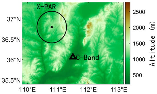
Figure 1.
The topography around the X-PAR and the nearest operational radar (C-band).
The original observed variables analyzed in this paper are ZH and ZDR. Finite impulse response (FIR) low-pass filtering with a 500 m window is used to suppress radial statistical fluctuations in ZH, ZDR, and the copolar correlation coefficient (ρhv). On the lowest two elevation layers, ZDR anomalies caused by partial occlusion are identified and removed by ρhv < 0.7. Other radar information, processing methods, and comparative studies of data reliability are described in [26]. In addition, note that no attenuation correction for rainfall areas is adopted for the radar data for the following two reasons:
- (1)
- The horizontal scale of the ZH core is only approximately 5 km, and there is no large-scale rainfall area passed through by the radar beams, so there is no obvious attenuation. Although there is inevitably attenuation to some extent on the far side of a radar beam when it passes through a convective core, such areas are less important to the study in this paper since the focused area with ZH core and ZDR columns are both on the near side of the X-PAR beams. The specific situation is shown in Section 2.4.
- (2)
- There are inevitably some large fluctuations in the differential phase shift in the weak echo area at the cloud edge, which makes it difficult to obtain a stable differential propagation phase when the continuous radial data on a radar beam are too short (e.g., for the target small-scale convective cell in this study). A forced correction based on that may instead contaminate the original structure of the cell.
As mentioned above, the C-band operational radar is used to evaluate the attenuation condition and the reliability of the X-band phased-array radar in Section 2.4.
2.2. Weather Conditions and Convective Cell Selection
On 8 July 2021, the 200 hPa jet stream and a 500 hPa trough were over Shanxi Province; additionally, the western Pacific subtropical high was located to the south of this region. Figure 2 shows the local weather conditions near the radar site obtained from ERA5 reanalysis data. Northwesterly winds dominate in the mid-upper troposphere, and the winds in the lower layers change from westerly to easterly and southeasterly after 09:00 UTC (Figure 2a). This wind shear condition is a potentially favorable condition for the maintenance of convection since it is conducive to the dislocation of an updraft and a downdraft. The convective available potential energy (CAPE, Figure 2b) shows medium convective instability with a maximum of over 1000 J km−1. Scattered convective cell storms appear in Xixian County after 05:00 UTC. The local weather modification department conducts hail suppression operations using anti-aircraft guns from 07:00 to 08:00 UTC and from 10:27 to 10:28 UTC, aiming at highly organized convective cells. There is no report of hail in the ground on this day.
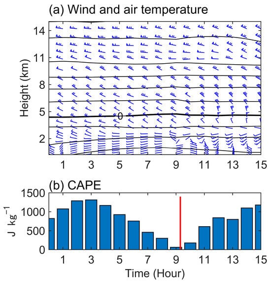
Figure 2.
Local weather conditions near the radar site from ERA5 reanalysis data on 8 July 2021: (a) wind and air temperature and (b) convective available potential energy (CAPE). The wind barb and contour lines in (a) represent horizontal wind and air temperature (with 10 °C intervals), respectively; the bold black line represents the 0 °C level (approximately 4.73 km height). The vertical red line in (b) represents the emerging moment (09:18 UTC) of the convective cell observed with the X-PAR. The local standard time is Beijing Time (UTC + 8), and the time used in this paper is UTC.
The analysis object selected in this paper is a strong and isolated convective cell storm that emerged in the clear sky after 09:00 and contained ZDR columns. This convective cell formed in a period with relatively low CAPE (Figure 2b), which might explain why it is an isolated one instead of a more active convective system with larger scale or multiple cells. Owing to the observation of the complete life cycle of this isolated convective cell, it is possible to find and confirm the coexistence of two ZDR columns in one convective cell. This phenomenon may be easily ignored in mesoscale convective systems where convective cells continue to form and dissipate.
2.3. Radar Variables for Analysis
The variables calculated from the original radar data are as follows:
- (1)
- Composite reflectivity (Ze). Triple linear interpolation is used to interpolate ZH in polar coordinates (elevation, azimuth, and radial distance) into a uniform grid of rectangular coordinates with a resolution of 100 m × 100 m × 100 m. The maximum value in the vertical direction is taken to form a horizontal distribution map to characterize the development and movement of the cloud system.
- (2)
- Composite ZDR in cold layers (ZDRC)/warm layers (ZDRW). Similar to the process of conducting Ze, grids at heights where the temperatures are less than 0 °C are used to derive the ZDRC for observing the horizontal positions of ZDR columns. Conversely, grids at heights where the temperatures are above 0 °C are used to derive the ZDRW for observing the horizontal positions of large raindrops at low levels. Note that sometimes the horizontal ice crystals in the cloud top and weak echo areas will lead to large ZDR. At such time ZDRC is not applicable for locating a ZDR column. However, most such weak echoes are not collected with the X-PAR used in this paper, so ZDRC still works.
- (3)
- Radial velocity divergence (RVD). The change rate of filtered VR along the radial direction is obtained by the central difference to obtain the RVD, which helps to diagnose vertical motion by showing the convergence and divergence distributions in a vertical structure [26]. The convergence area shown by RVD indicates an updraft and corresponds to a ZDR column in a recent study [27]. Although a 3D wind field retrieval algorithm can retrieve strong updrafts [28] and seems better for dynamic analysis, such algorithms often need to introduce additional assumptions, and it is often difficult to obtain in situ observations of the vertical airflow in a mesoscale or smaller convective system for verifying a retrieved updraft or downdraft. Compared with that, RVD is not limited by additional assumptions and is considered to provide direct evidence of a dynamic structure in a convective precipitation cloud. A previous similar variable for diagnosing dynamic structure is storm-top divergence (STD) [14], but it is mainly used in time series analysis. In this paper, the comparability of the RVD and the simulated vertical dynamic structure with a cloud model is shown.
Physical characteristic retrievals such as particle size distribution and 3D wind are not applied in this paper since the empirical assumptions for the above retrieval are not easily verified in severe convective clouds. In addition, the hydrometeor classification based on radar polarimetric variables is not used for a main analysis object due to its limitations and uncertainty [29]; it is only briefly discussed in Section 3.5.
2.4. Radar Attenuation Evaluation
Taking the data in the middle stages as an example, the relative positions of the X-PAR and the C-band radar and the surrounding terrain are shown in Figure 3a, where the target cloud is east of the X-PAR and northwest of the C-band radar. The far side of the X-PAR beams is approximately the near side of the C-band radar. Since there is theoretical attenuation in the C-band, whether there is obvious attenuation in the C-band radar needs to be clarified first. Regardless of the beam blocks, there is no large-scale precipitation between the target cloud and the C-band radar, and the scale of the target cloud is small, so it can be deemed that there is no considerable rainfall attenuation on the near side of the 4th PPI of the C-band radar before it detected the target cloud. The higher elevation PPIs of the C-band may reach or are beyond the cloud top of the target cloud. Therefore, at least the 4th-level PPI of the C-band radar can be used for quantitative assessment of the attenuation condition of the X-PAR.
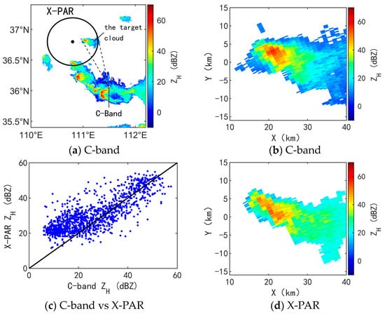
Figure 3.
Example of a comparison of X-PAR and C-band radar on the same PPI surface. Data near 09:51 are used from these two radars. (a) ZH in the original 4th-level PPI of the C-band radar at 3.4° elevation. (b) The same as (a) but zoomed at the target cloud, and the X and Y coordinates are converted to be relative to the X-PAR. (c) The scatter plot of data in (b,d), where both of them have valid data points. (d) ZH of X-PAR that was interpolated to the same PPI surface of (b). The dashed lines in (a) mark beam ranges of the azimuth of the C-band radar, which cover the target cloud.
A quantitative comparison is shown in Figure 3b–d, where the X-PAR data are interpolated into the original 4th-level PPI surface. There is a less weak echo in the echo edge of the X-PAR due to its lower sensitivity. However, the shapes of these two echoes are similar, and some parts of the X-PAR still seem higher. The scatter plot in Figure 3c shows that the reflectivities from these two radars are basically consistent from 30 to 60 dBZ, where the scattered points are evenly distributed on both sides of the reference line. In addition, the reflectivity of the X-PAR is larger than that of the C-band for the weaker part of the echo, which cannot be fully explained at present. Considering that the altitudes in Figure 3b,d are 5~7 km, where the temperature is below 0 °C and ice crystals and snowflakes may exist over the periphery of the upper level of convection, some intrinsic differences may exist due to radar band and particle orientation. In addition, a lower signal-to-noise ratio at a farther distance or partial beam blocking may cause the weaker part mentioned above, though these possibilities cannot be easily evaluated currently. However, no obvious attenuation characteristic in the X-PAR is found over convection areas.
Another issue that needs to be checked is whether there is an actual ZDR column or if the observed feature is an artifact. Figure 4 shows an example. The RHI at 72° azimuth (Figure 4b,e) passes through the main ZDR column (stronger one), where a vertical structure with a high ZDR value exceeding 6 km height is found, but it is slightly close to the cloud edge. A clearer vertical structure is seen in the RHI at 79.2° azimuth (Figure 4f), where the radar beams pass through the center of the secondary ZDR column and edge of the main ZDR column without passing through any other cloud in advance. These two isolated high ZDR value areas both exceed a height of 6 km, and they are not close to the cloud edge, so they are certainly not cluttered near edges. Therefore, the result of obtaining two ZDR columns is reliable. The possible attenuation in the far end of the radar beam, such as the easternmost part of Figure 4a, does not affect the analysis of ZDR columns around the convection area in this paper.
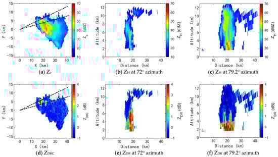
Figure 4.
Examples of original RHIs observed with the X-PAR, which contain ZDR columns: (a) Ze and the direction mark of the RHIs; (b) ZH at 72° azimuth; and (c) ZH at 79.2° azimuth; (d–f) are the same as (a–c) but for ZDRC or ZDR. The dashed lines in (a,d) represent 72° (upper) and 79.2° (lower) azimuths.
2.5. The Cloud Model
2.5.1. Brief Introduction
A three-dimensional convective storm model (IAP CSM3D) [30,31] is used to perform numerical simulations. This model is a compressive cloud model for ideal simulation experiments, whose background field is set by a vertical atmospheric profile. A convection can be triggered by a thermal perturbation or a cool pool outflow, which need to be manually set. The microphysical schemes are based on bulk water techniques. There is a single-moment scheme for cloud drops and a two-moment scheme for the other six classes of hydrometeors, including raindrops, ice crystals, snow, frozen drops, graupel, and hail. In addition, there is a seeding ice crystal class that is another independent class when artificial seeding issues are studied. A frozen drop is defined to be formed by raindrop nucleation or raindrops collected by ice crystals and snow, which both contribute to raindrop freezing. The frozen drop class is separated from the traditional graupel class to better characterize the formation of different hail embryos. Other information about the schemes used in the model is given in [30,32].
The purpose of using this cloud model is that when the macrocharacteristics of the simulated convective cell are similar to the observations with the X-PAR, more reliable dynamic and microphysical processes can be obtained and analyzed using the combination of observation and simulation rather than only using radar signals. There are three aspects to compare their similarity: ZH, ZDR, and horizontal (or quasihorizontal) divergence. The ZH is easy to compare since most numerical models produce a general Z where the dielectric parameters and densities of different hydrometeors are considered in the calculation of spherical equivalent reflectivity. The simulated horizontal wind divergence (HWD) is compared with the observed RVD. Although there are inherent differences between HWD and RVD in definitions, some basic dynamic characteristics can be obtained without additional assumptions. The scheme for obtaining ZDR is described in the following section.
2.5.2. ZDR Simulation Scheme
To obtain simulated ZDR, both horizontal and vertical reflectivity (ZH and ZV) are necessary, which are related to microphysical characteristics and distributions. Details of the two-moment bulk water scheme for raindrops used in the cloud model are seen in [32]. The raindrop size distribution (RSD) is represented by a classical gamma distribution [33], as shown in Equation (1):
where N(D) (unit: m−3 m−1) is the number density of the RSD over equivalent spherical diameter D (unit: m); N0 (unit: m−3 m−1−μ) is the number concentration parameter of the RSD; μ (dimensionless, fixed to 2 in the cloud model) is the shape parameter of the RSD; and β (unit: m−1) is the scale parameter of the RSD. Since μ is fixed, the remaining two independent parameters (N0 and β) are estimated with simulated variables in the cloud model (Equations (2) and (3)):
where ρ (unit: g m−3) is the density of air; ρL (fixed to 106 g m−3) is the density of liquid water; Q (unit: g g−1) is the simulated mixing ratio of raindrops; and NT (unit: g−1) is the simulated total number concentration of raindrops.
Using the parameters above, the RSD can be obtained. Then, the results from a forward calculation based on radar scattering numerical simulation and a specific shape-size relation [34] can be used to obtain both the horizontal and vertical reflectivity (ZH and ZV) of raindrops as follows:
where Zh (or Zv), with lowercase subscripts, has linear units (mm6/m3), and ZH (or ZV), with uppercase subscripts, are in log units (dBZ). Kw is associated with the dielectric property (Kw = (ε − 1)/(ε + 2)). λ (unit: m) is the wavelength of the radar. Shh,vv is the backscattering amplitude of a single hydrometeor particle in a horizontal or vertical channel. Dmin and Dmax are the lower and upper limits of the RSD, which are set to 0.1 and 9 mm, and the interval is 0.1 mm. Since the ZDR contributed by other ice-phase particles due to specific shapes and orientations is not the focus of this paper, the ZH and ZV of other hydrometeor classes except raindrops are set to be the same Z derived from spherical equivalent reflectivity. Then, the ZDR (unit: dB) of a grid in the model is obtained as follows:
where Z(other classes) is the sum of Z (unit: mm6/m3) of other hydrometeor classes.
There are several problems with ZDR simulation that need to be explained:
- (1)
- The numerical model cannot reflect the partial melting state of ice phase particles. One difference is that in the area where there may be melting graupel particles falling into lower levels, observations will show that the ZDR increases from top to bottom, while the simulation results may show a ZDR valley near 0 dB compared with both sides in the horizontal direction. This will make the simulated image appear to be spatially discontinuous. However, the distributions of relatively large ZDR centers and ZDR columns are still comparable to the observation results.
- (2)
- Due to the influence of numerical techniques, there are occasional places where Q and N are very small at the edge of the upper raindrop areas (e.g., closer to the lower limit of the calculation precision), and when N is much smaller, it will lead to a large average diameter of raindrops, resulting in an abnormally large value of ZDR and a discontinuous distribution around it. This problem cannot yet be completely solved, but since it does not affect the overall viewing of the vertical section, it has no essential impact on the analysis of this paper.
- (3)
- The simulated ZDR value is smaller than the observation. This may be limited by the inherent limitations of the two-moment scheme used in the model. A similar result that also has a smaller simulated ZDR can be found in another numerical model [35]. Among the simulation results, the ZDR values of the warm layer are slightly smaller (the observation is usually 1~4 dB, and the simulation is usually 1~2 dB), while those at the ZDR column position in the cold layer are much smaller (the observation is usually 1~3 dB, and the simulation is usually less than 1 dB). However, in view of the fact that the position of the ZDR column in the simulation results can be close to the observation, this problem has limited influence on the analysis in this paper. In addition, this problem will be briefly discussed in the last part of Section 4.
- (4)
- Before using the cloud model, some mesoscale simulation experiments were carried out using the Weather Research and Forecasting (WRF) model, including different microphysical schemes. However, it is challenging to accurately simulate a small-scale convective cell originating from the clear sky using a mesoscale model. Most of these simulation results did not provide a comparable convective cell when they were compared with the observation. On the other hand, a spectral bin microphysical model such as that used by Kumjian et al. [11] may lead to a long test cycle for numerical calculation. These are the reasons why a cloud model based on a two-moment bulk water scheme is used in this paper instead of using the more popular WRF or other bin models.
2.5.3. Model Setting
The model is set to a grid with 120 × 120 × 100 gridpoints. The horizontal/vertical resolutions are set to 300 m and 150 m. The bottom and top air pressures are 975 hPa and 120 hPa, respectively. The method for triggering convection is thermal perturbation. The central strength of the thermal perturbation is 1 K, the horizontal and vertical radii are 2.4 km and 3.9 km, respectively, and the height of its core is at the −0.5 °C level. The initial cloud concentration is set to 100 cm−3. The small time step for the microphysical process is 0.2 s, and the larger time step for a whole-time integration is 1 s. The selected background vertical profile is basically the same as that shown at 10:00 UTC in Figure 2, but the relative humidity in lower levels is enlarged from 30 % to 70 % since the original conditions are too dry to produce a convective cell with high ZH (e.g., ZH greater than 50 dBZ).
3. Results
3.1. Overview of the Convective Cell Evolution
Four moments for representing typical stages are selected to demonstrate the evolution of the target convective cell (Figure 5), including the time the cloud emerged, the time containing the main ZDR column in the early stages, the time when the secondary ZDR column was strongest, and the time after the secondary ZDR column disappeared. To better describe the location of various echo characteristics, the moving direction of the convective cell is defined as its visual moving direction during the entire study period (this direction is shown in Figure 5, basically south and a little east), and the rear and front side are defined according to this moving direction. These relative locations are marked in the upper left of Figure 5.
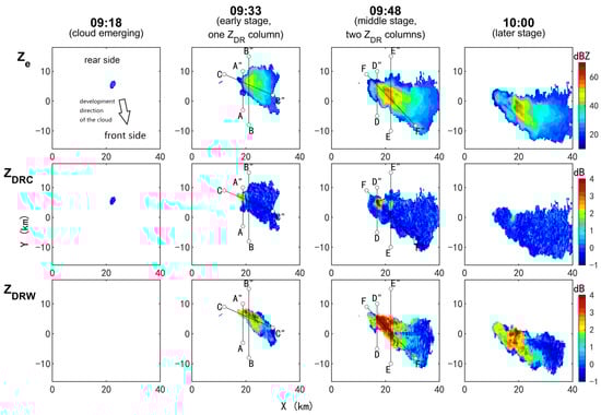
Figure 5.
Evolution of Ze, ZDRC, and ZDRw observed with X-PAR. X and Y represent west–east and south–north distances relative to the radar site. Lines A–F are the locations of selected typical vertical profiles, which will be analyzed in the following. The front side and rear side relative to the moving direction of the cloud are marked in the upper left sub-figure. The time is UTC.
As shown in Figure 5, a weak echo approximately 2 km in diameter emerged in the upper air at 09:18 UTC. This echo grew into a cell storm with a diameter exceeding 10 km within 15 min (09:33 UTC); the maximum Ze exceeded 60 dBZ in half an hour (09:48 UTC). Subsequently, the strong center weakened, and there were scattered multiple weak centers in the later stages (10:00 UTC). In the early stages (09:33), an area with a ZDRC close to 3 dB appeared on the west side of the cell (right side relative to the moving direction of the cloud), corresponding to a ZDR column. A relatively narrow band of ZDRW showed that only a part of the cloud was grounded at this time, and the value of ZDRW indicated large raindrops falling in the cell front (09:33 UTC). In the middle stages (09:48), two ZDR columns coexisted. One column existed previously on the west side, and it was further enhanced to 4 dB (hereinafter referred to as the main ZDR column); the other was the weaker ZDR column at the rear of the high Ze area (hereinafter referred to as the secondary ZDR column). ZDRW showed an entire high ZDR area in the warm layer, indicating that large raindrops were produced everywhere in the warm layer of the cloud (09:48 UTC). Later, the secondary ZDR column disappeared, and the main ZDR column was still visible but became weaker (10:00 UTC).
Figure 6 shows the simulated results using a similar plotting and time selection method as the X-PAR observations (Figure 5). There are inevitable differences between the observation and the simulation since the selected background field and physical schemes in the numerical cloud model may be different to some extent from the real situation. The main difference between the observation and the simulation are as follows.
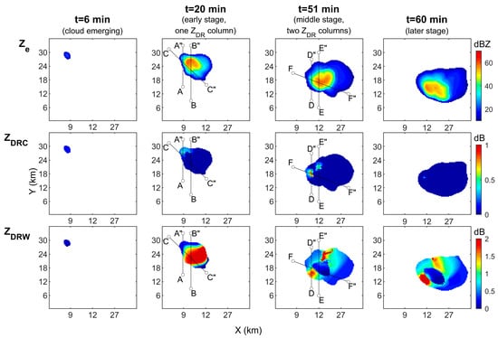
Figure 6.
Evolution of Ze, ZDRC, and ZDRW simulated with the cloud model. X and Y represent west–east and south–north distances of the model domain. Lines A–F are the locations of selected typical vertical profiles, which will be analyzed in the following.
- (1)
- The moving direction of the simulated cell is more eastward.
- (2)
- The simulated ZH is stronger in the early stages, and it is weaker in later stages, but the most visual difference is no more than 10 dBZ.
- (3)
- The emerging time of the secondary ZDR column is different. In the observation, the time lag between the two ZDR columns’ emergence is approximately 20 min, while in the simulation, the value is 30 min.
- (4)
- As mentioned in Section 2.5.2, the magnitude of the simulated ZDR is lower than the observation.
However, the cloud scale, extension direction, and location of the two ZDR columns are similar. In the following part, based on the same moments of the early and middle stages shown in Figure 5, the vertical profiles of both the observation and the simulation are compared, and signals reflecting dynamic and microphysical characteristics are combined with the simulated wind and hydrometeor fields for analysis.
3.2. Typical Vertical Structures
3.2.1. The Selection of Vertical Profiles
Based on the overall macro distribution in the early and middle stages (Figure 5 and Figure 6), typical interpolated vertical profiles are selected to further analyze the dynamic and microphysical characteristics around the two ZDR columns, as well as their formation mechanisms. Information on the six profiles from AA″ to FF″ represented in Figure 5 and Figure 6 is shown in Table 2. Profiles AA″ and CC″ are selected to check the main ZDR column in the early stages, while profiles DD″ and FF″ are for the middle stages. In addition, profiles BB″ and EE″ are comparable for determining why the secondary ZDR column does not exist in the early stages and appears later.
Table 2.
Information of interpolated profiles AA″ to FF″.
3.2.2. The Early Stages
In profiles AA″ (Figure 7), the observation and simulation are basically consistent. The strength and shape of ZH are similar, which are south-leaning and toward the cell’s front, ungrounded, and less than 40 dBZ. Although the simulated ZDR value is small, as mentioned in Section 2.5.2, it still shows a ZDR column extending from the warm layer to the cold layer. Both RVD and HWD show a convergence area extending from the warm layer to the cold layer. It can be seen from the simulated wind field that this convergence area is formed by the confluence of the low-level inflow and the middle-level airflow and corresponds to the bottom of the updraft core. The updraft is mainly distributed in the cold layer, and the maximum updraft velocity is more than 20 m s−1. In addition, the HWD shows that the upper-level divergence is divided into two parts, including a divergence formed by the acceleration of the northern upper-level air flowing into the south-leaning updraft center and a divergence area of the upper-level outflow in the south. Although the RVD does not have such a clear block, it also shows that the upper air is almost a divergent area. According to the above characteristics of low-level convergence and high-level divergence, it can be inferred that there is actually an updraft at the main ZDR column in the early stage.
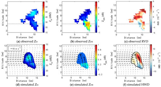
Figure 7.
Variables in profiles AA″ observed with the X-PAR and simulated with the cloud model. (a) Observed ZH, (b) observed ZDR, (c) observed RVD, (d) simulated ZH, (e) simulated ZDR, and (f) simulated HWD. The dashed lines represent the height where the background air temperature is 0 °C. The outlines of the simulated echo are limited to 10 dBZ. Black vectors are the simulated wind field.
For profiles BB″ (Figure 8), although the observations and simulations are not as similar as in profiles AA″, there are still some things that can be mutually confirmed. ZH shows that the convective cell tilts slightly backward. The large values of ZDR are all below the 0 °C level, and no obvious ZDR column is observed. The RVD and HWD show that although there is convergence in the middle layers and divergence in the upper layers, there is also a divergence center at a height of 2 km near the ground. This divergence distribution is different from the pattern corresponding to the strong upward flow in profiles AA″. From the simulated wind field, the warm layer is dominated by downdraft. The airflow in the rear middle layer can also flow into the updraft area of the convective cell, but it is mainly concentrated in the rear of the cold layer, rather than the updraft in the warm layer of the cloud center as in profiles AA″.
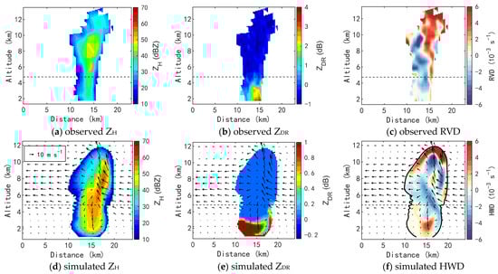
Figure 8.
Same as Figure 7 but for profiles BB″.
A more complete updraft–downdraft circulation is seen in profiles CC″ (Figure 9). The simulated updraft area is at the edge of the cloud body on the left side of the image (actually on the west side, corresponding to the right rear side of the moving direction of the cloud), corresponding to the main ZDR column. The weak echo near the 0 °C layer has a structure similar to an overhang in both observation and simulation, which is commonly deemed to be an updraft indicator. The downdraft area is in the downwind direction of the high-level wind and near the ZH core. RVD and HWD show that there are divergent areas on the outmost layers and convergent areas on the inner layer where the main ZDR column stands. The simulated wind field shows that the divergence area of the upper outer layer may be caused by the acceleration of the air when it flows into the inclined updraft zone. The convergence areas include two parts. One is a convergence of warm layer flow, and the other is the convergence of cold layers around the updraft center. Although the RVD shows a more complex distribution in the upper air than the HWD, which is not easy to explain at present, the side where the main ZDR column stands has the characteristics of low-level convergence and high-level divergence in both RVD and HWD, indicating that there is a strong updraft. In addition, the hydrometeors formed at the updraft corresponding to the main ZDR column could be transported downstream with the high-level wind and then fall, which not only did not interfere with the original updraft but also enhanced the updraft–downdraft circulation mentioned above.
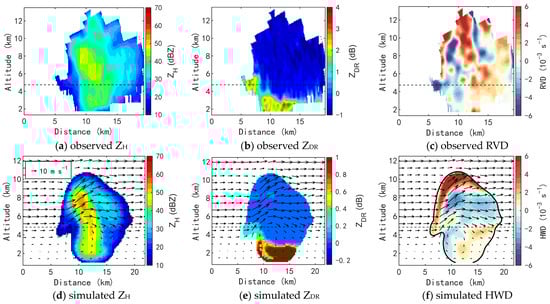
Figure 9.
Same as Figure 7 but for profiles CC″.
3.2.3. The Middle Stages
The profiles DD″ (Figure 10) in the middle stages have similarities with the earlier profiles AA″. The forward-leaning ZH core is still not very strong, although it exceeds 40 dBZ. Although there are abnormally large values and discontinuities in the simulated ZDR, as mentioned in Section 2.5.2 (Figure 10e), where the abnormally large values are mainly located in the front of the cell and the top of the ZDR column, a structure of the ZDR column can still be seen. Compared with the early stages (Figure 7b,e), the observed and simulated ZDR are larger, and the simulation shows that the ZDR column becomes located below and behind the updraft. This indicates that larger raindrops are falling. Both RVD and HWD show a convergence center in warm layers and divergence centers in cold layers. Although there is a part of echo grounded and divergence near the ground at the position of the main ZDR column, the front low-level inflow can still converge with the rear middle-level air flow below the 0 °C layer. This is conducive to the maintenance of the strong updraft through the cold layer and the warm layer.
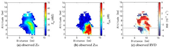
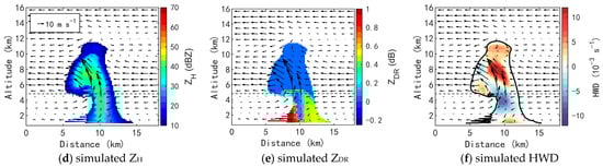
Figure 10.
Same as Figure 7 but for profiles DD″.
In profiles EE″ (Figure 11), the simulated ZH is higher than that in the observation. The high-level strong echo has a backward overhang, which is not obvious in the observation, but both of them are similar to profiles BB″ at the early stages. RVD and HWD show divergence in the bottom layers and the rear of the cold layer, and there is a convergence center in the warm layer between the two divergence areas mentioned above. The simulated wind field shows a strong updraft corresponding to the location of the secondary ZDR column. This updraft starts from the convergence center and extends to the cloud top. Compared with profiles BB″ without a ZDR column in the early stage, the bottom divergence outflow caused by precipitation is more obvious. Therefore, a reasonable inference is that the middle and low air at the rear is forced to be lifted by the divergent outflow, forming a deeper updraft that starts from warm layers and connects the existing updraft in cold layers. This helps the formation of the secondary ZDR column. In addition, there is a large ZDR area near the 0 °C layer at the upper part of the ZDR column, which is separated from large ZDR areas on low levels. This distribution is less obvious in the simulation (Figure 11e) but more obvious in the observation (Figure 11b). This large ZDR area may correspond to two sources of large raindrops. One is the collision and coalescence process among cloud drops and raindrops in the cold layers, and the other one is the melting of ice particles and the collision in warm rain layers.
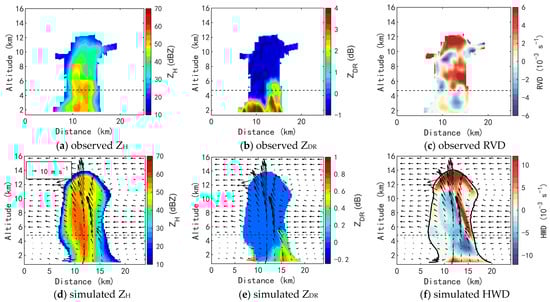
Figure 11.
Same as Figure 7 but for profiles EE″.
As shown in profiles FF″ (Figure 12), although there are similar structures in echo and divergence compared with the earlier profiles CC″ (Figure 9), the cloud scale is further extended, and the bottom divergence zone is distributed at a farther place downstream. This leads to the bottom divergence outflow not connecting with the main ZDR column and updraft area to create the convergence region as before. This may be one of the reasons why the system is no longer enhanced and begins to weaken.
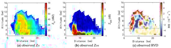
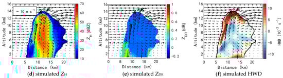
Figure 12.
Same as Figure 7 but for profiles FF″.
In addition, the difference in temporal changes between the observed and simulated ZDR changes needs to be explained. The observed ZDR in the middle stages (Figure 12b) is obviously larger than that in the early stages (Figure 9b) on both the main ZDR column area and the lower levels, indicating that various types of hydrometeor particles are growing. However, the simulated ZDR does not appear to be larger at the lower levels in the middle stages. A similar situation is mentioned in Section 2.5.2. Since there is no simulation to reflect a melting graupel, the simulated ZDR at the lower level in the middle stages is closer to 0 when a melting graupel is present. This is different from the early stages when the raindrops were dominant in the low levels.
3.3. Typical Horizontal Structures
On the horizontal sections near the 0 °C level, the shape of the ZDR column is worth noting. In the early stages (Figure 13), the main ZDR column is located at the rear end of the extended direction of the cloud. The shape of this ZDR column is similar to “C” or a flipped “D” with the opening toward the ZH core and the direction of cloud extension. In the simulated vertical air velocity (W, Figure 13c), the updraft core at this height also presents a C-shaped distribution, and its opening direction corresponds to a large area of downdraft downstream. Note that only half of both the updraft core and the ZDR column area are overlapping. One possible explanation is that another part of the updraft core corresponds to the forming ice-phase particles, which will be confirmed in the next section. Except for the non-overlapping parts mentioned above, a C-shaped ZDR column can be a signal for indicating the updraft area and the nearby downdraft area.
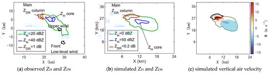
Figure 13.
Typical horizontal distribution in the early stages. The selected height is where the background temperature is near 0 °C. (a) Observed ZH and ZDR; (b) simulated ZH and ZDR; and (c) simulated vertical air velocity. The thinner black line in (c) is 0 dBZ for ZH, and the thicker black line is 0.2 dB for ZDR, which are the same in (b).
In the middle stages, the C shape of the main ZDR column is more obvious in both the observation and simulation results (Figure 14a,b). The secondary ZDR column is located at the rear of the ZH core, while the updraft also splits into two adjacent regions at the 0 °C level height. One thing that needs to be mentioned is that the secondary ZDR column appears to have split from one side of the C-shaped main ZDR column before the middle stages, as shown in Figure 15. Combined with the analysis in Section 3.2.3, in addition to the lower-level divergent outflow, the formation of the secondary ZDR column may also be affected by the downstream extension of the upper-level updraft core.
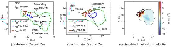
Figure 14.
Same as Figure 13 but for the middle stages. The black thin line in (c) is 0 dBZ for ZH, and the thicker black line is 0.2 dB for ZDR, which are the same in (b).
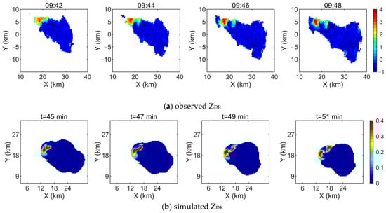
Figure 15.
Demonstration of the secondary ZDR column splitting from the main ZDR column: (a) observed ZDR and (b) simulated ZDR. The unit of the shading is dB. The selected height is where the background temperature is near 0 °C. The depicted outlines of the cloud correspond to ZH = 0 dBZ.
In addition, it should be pointed out that the above C-shaped ZDR column is opposite to the ZDR column patterns in previous conceptual models and real observations of a supercell [3,36,37] and [17] (p. 281), though the authors of these studies did not make a specific discussion on the C-shaped ZDR column. In a supercell storm, the opening side of the “C” corresponding to a ZDR column opens in the opposite direction of the cloud extension. This distribution corresponds to the position of an updraft, which is essentially different from the one in this paper. The main updraft area of a supercell is located in the front, rather than in the lateral and rear sides of the convective cell, as shown in this paper. This may also be one of the reasons for the essential differences in their strength and life span, but more research is necessary to figure this out in the future.
3.4. Microphysical Characteristics around the Two ZDR Columns
The simulation provides microphysical processes and hydrometeor fields, but in view of the variety of these fields, only their relative position distribution is shown in Figure 16. The contour scales for reference are seen in Table 3. In addition, for the convenience of viewing these images, ice crystals and snow are shown as one class that have relatively similar properties; graupel and hail are also combined since there is less hail in the result and no real report of a hail event.
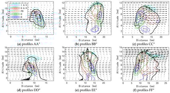
Figure 16.
Relative distribution of different hydrometeors in profiles (a) AA″, (b) BB″, (c) CC″, (d) DD″, (e) EE″, and (f) FF″. The hydrometeors include ice crystals (I), snow (S), graupel (G), hail (H), frozen drops (FD), cloud drops (C)l and raindrops (R). The bold black lines are the outlines of ZH = 10 dBZ. Colored contour lines are based on simulated water content and are automatically produced according to their own value range in a specific time and profile instead of a fixed value. The scales of these contour lines are seen in Table 3.
Table 3.
The scales of contour lines in Figure 16. The unit is g m3. For three contour lines of each class of hydrometeor, values in this table show the lowest and highest.
In the early stages, the position of the main ZDR column is dominated by uplifting condensed cloud droplets and converted raindrops (Figure 16a). The updraft and the main raindrop areas extend from the warm level to the cold level and near the cloud top. The large value center of raindrops is at the 7 km height in the cold layer, and the frozen droplets mainly form here. In the other profiles (Figure 16b,c), there are two centers of raindrops. One is located in the strong updraft area in the cold layer; the other is located in the lower layer, which is generated by the melting of frozen droplets. In addition, the center of the graupel is in the downwind direction of the raindrop area on the upper levels, and it is closer to the center of the convective cell. This indicates that supercooled raindrops will be collected by the graupel to promote its growth. In the middle stages, the range of graupel in cold layers expands (Figure 16d) and extends down to the warm layer and melts (Figure 16e,f). The center of the low-level rain is grounded due to the melting precipitation process. This explains the enhancement in bottom divergence in the middle stages in Section 3.2.3.
For the formation mechanism of the ZDR columns, it can only be known from Figure 16 that a large number of raindrops are converted from cloud droplets in the cold layer, but it is still not clear whether raindrops are transported from the warm layer to the cold layer by the updraft. For this reason, the vertical flux of raindrops is calculated as follows:
where VT is the mean terminal velocity of raindrops given in the cloud model. Figure 17 shows that, except for the location without a ZDR column at the early stages (Figure 17b), there is an obvious upward flux of raindrops from the warm layer to the cold layer. Therefore, the ZDR columns can be considered to be caused by both the condensation and collision growth of liquid droplets in the cold layer and the upward transportation of raindrops in the warm layer.
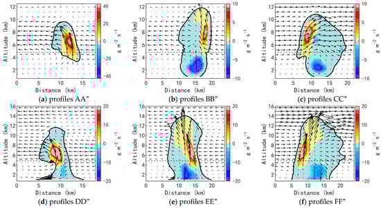
Figure 17.
Same as Figure 16 but for the simulated vertical flux of the water content of raindrops.
3.5. Other Characteristics Related to Radar Polarization
Hydrometeor classification (HC) is a famous use of dual-polarization radar for both research and meteorological services. An important issue is whether the HC result in the upper air is reliable, especially in severe convection where in situ observations are difficult to obtain. Figure 18 shows a set of HC results, which is derived from the fuzzy logic scheme of Feng et al. [38] and has been used in previous studies [26,39]. Although the observation is still lacking, the hydrometeor classes in the simulation (Figure 16) and HC can mutually confirm each other. For example, HC shows supercooled water near the main ZDR column in the early stages (Figure 18a), and a graupel area above 8 km height is very similar to the simulation (Figure 16a). In addition, there are many similar distributions between the simulation and the HC, including the graupel areas dominant in the most upper air of the convection, the snow and ice crystals on the top and outer layers, and the “rain & hail” class in the lower level at the later stages, which corresponds to the melting of hail, graupel, and frozen drop. In general, these HC results have a certain rationality. However, the actual microphysical process in the cold layer usually involves different hydrometeors and their transformation in the same space, and the HC algorithm does not have the capacity to reflect that. Therefore, its use in microphysical research is limited, and it is not used as a main analysis approach in this paper.
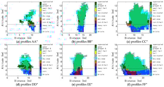
Figure 18.
Same as Figure 16 but for the hydrometeor classification retrieved from X-PAR data.
In addition, ρhv and differential propagation phase shift (KDP) are common analysis objects that show fingerprints of microphysical processes. For ρhv, some typical vertical profiles show values near and lower than 0.9 at the top of the two ZDR columns in the middle stages. This reflects a nonuniformity of the phase and shape of particles, and it is consistent with the processes in Figure 16, where raindrops can be transformed into frozen drops or collected by different ice particles. The presence of hail is also known to decrease ρhv. However, since there are many influencing factors on a low ρhv, it is not easy to fully explain all low-value areas. For KDP, large values concentrate at low levels, which reflect high liquid water content, and some typical vertical profiles show KDP columns similar to the ZDR columns. In general, these features were reflected in the HC results (Figure 18). Therefore, the images of ρhv and KDP are not displayed here.
4. Discussion
The formation and maintenance conditions of the secondary ZDR column are very different from those of the main ZDR column. The updraft corresponding to the secondary ZDR column is partly due to the forcing of precipitation with downdraft at the rear of the convective core in the middle stages, while the main ZDR column forms under the convergent flow from both sides relative to the moving direction of the cell. In an environment with considerable wind shear, the hydrometeors in the middle and upper layers are transported to the downwind area, which makes the precipitation with downdrafts stagger with the main updraft area, so that the main ZDR column maintains for a longer time; as the precipitation weakens after the middle stages, the formation and maintenance conditions of the secondary ZDR column gradually disappear, which leads to its shorter maintenance time. Since the secondary ZDR column does not correspond to the formation of a new convection or an enhancement in the original convection, it should be regarded as a by-product of a convection at the middle stages rather than an indicator of stronger weather. This may also be one of the potential factors that may interfere with the judgment of the situation through the ZDR column.
The weaker values of ZDR within the ZDR column imply the underestimation of supercooled raindrop size using the cloud model. This provides clues for improving the common two-moment microphysical schemes. For example, there may be a difference in RSDs between the raindrops transformed from cloud droplets in the cold layer and those transported from the warm layer by an updraft. At this time, the collision between these two parts of raindrops may not be the continuous translation of a peak of the RSD, which makes the traditional two-moment scheme difficult to characterize in this situation. A possible solution may be to treat cloud-transformed rain and melt-formed rain as two individual categories in the numerical model.
5. Conclusions
Benefiting from the dual polarization X-PAR capable of fast scanning, the complete lifetime of a cell storm, which emerged from the clear sky and contained two ZDR columns simultaneously, was observed. Since a ZDR column was previously considered to correspond to an updraft, the coexistence of two ZDR columns in a single convective cell implies a certain complexity of the dynamic structure, which is different from the single updraft structure in the common convective cell conceptual model. Analysis of typical spatial structures at different stages was studied using X-PAR observations and cloud model simulations. The main conclusions were as follows:
- (1)
- The main ZDR column is located in the opposite direction of the cloud extension and is on the right side of the ZH core relative to the cloud development. Under the influence of the convergence of low-level inflow in the front- and middle-level flow at the rear, the main ZDR column lasts from the early stages to the later stages of the convective cell.
- (2)
- The secondary ZDR column is at the rear of the horizontal reflectivity (ZH) core. It mainly exists in the middle stages, and its existence time is shorter. The middle and low air at the rear is forced upward by the divergent outflow of the precipitation in the middle stages, which may be one of the formation causes of the secondary ZDR column.
- (3)
- The studied convective cell was born under a wind shear condition, where the wind directions in the lower and middle layers are opposite, and this is a known favorable condition for the maintenance of convection since it is conducive to the dislocation of an updraft and a downdraft. Along the cloud extension direction in the early stages, some factors are good for the maintenance of a specific circulation, including the updraft at the main ZDR column area, the hydrometeors transported downstream in the cold layer and falling down away from the updraft, and a part of the divergent flow near the surface converging with the inflow to maintain the updraft.
- (4)
- Both ZDR columns correspond to an updraft from the warm layer to the cold layer. Along these updrafts, there are raindrops converted from cloud drops in the cold layer and originating from the upward flux of raindrops, indicating two key sources for raindrops to form a ZDR column.
The above mechanism may also exist in other common mesoscale convective systems, but it may be neglected in previous studies because it is not easy to confirm two ZDR columns coexist in a single cell when there are many convective cells and many ZDR columns with different life periods. Owing to non-interference from other convective cells, the characteristics and formation mechanism of these two ZDR columns are better studied than in a multicell system. However, it can be inferred that similar phenomena may also be found in previous data under a targeted review.
In addition, some diagnostic features were found. The C-shaped ZDR column near the ZH core in a horizontal section indicates an updraft area near the downdraft area. The observed RVD and simulated HWD are comparable and can indicate the updraft by the convergence at low levels and divergence at upper levels. However, in-depth studies should be conducted based on fully verifying the retrieval results of dynamic and microphysical characteristics in combination with various observations in the future.
Author Contributions
Conceptualization, G.R. and Y.S.; methodology, Y.S. and H.X.; software, Y.D. and Y.Y.; validation, Y.D. and Y.Y.; formal analysis, G.R. and H.S.; investigation, G.R. and Y.S.; resources, H.S. and H.X.; data curation, Y.D. and Y.Y.; writing—original draft preparation, G.R. and Y.S.; writing—review and editing, H.S., Y.Y., and H.X.; visualization, G.R. and Y.D.; supervision, H.S. and H.X.; project administration, Y.S. and H.X.; funding acquisition, G.R., Y.S., and H.X. All authors have read and agreed to the published version of the manuscript.
Funding
This research was supported in part by the Central Guidance on Local Science and Technology Development Fund (grant no. YDZJSX2021B017), the National Natural Science Foundation of China (grant no. 42105127), the National Key Research and Development Plan of China (grant no. 2019YFC1510304), the Key Research and Development Plan of Shanxi Province (grant no. 202202130501020), the Qiankehe Support (grant no. 2023YIBAN193), the Research and Experiment on the Construction Project of Weather Modification Ability in Central China (grant no. ZQC-T22254), and the Science and Technology Project of Henan Science and Technology Department (grant no. 232102320013).
Data Availability Statement
Data are contained within the article.
Conflicts of Interest
The authors declare no conflicts of interest.
References
- Illingworth, A.J.; Goddard, J.W.F.; Cherry, S.M. Polarization radar studies of precipitation development in convective storms. Q. J. R. Meteorol. Soc. 1987, 113, 469–489. [Google Scholar] [CrossRef]
- Conway, J.W.; Zrnic, D.S. A study of embryo production and hail growth using dual-doppler and multiparameter radars. Mon. Weather Rev. 1993, 121, 2511–2528. [Google Scholar] [CrossRef]
- Kumjian, M.R.; Ryzhkov, A.V. Polarimetric signatures in supercell thunderstorms. J. Appl. Meteorol. Climatol. 2008, 47, 1940–1961. [Google Scholar] [CrossRef]
- Hall, M.P.M.; Cherry, S.M.; Goddard, J.W.F.; Kennedy, G.R. Rain drop sizes and rainfall rate measured by dual-polarization radar. Nature 1980, 285, 195–198. [Google Scholar] [CrossRef]
- Hall, M.P.M.; Goddard, J.W.F.; Cherry, S.M. Identification of hydrometeors and other targets by dual-polarization radar. Radio Sci. 1984, 19, 132–140. [Google Scholar] [CrossRef]
- Tuttle, J.D.; Bringi, V.N.; Orville, H.D.; Kopp, F.J. Multiparameter radar study of a microburst—Comparison with model results. J. Atmos. Sci. 1989, 46, 601–620. [Google Scholar] [CrossRef][Green Version]
- Ilotoviz, E.; Khain, A.; Ryzhkov, A.V.; Snyder, J.C. Relationship between Aerosols, Hail Microphysics, and ZDR Columns. J. Atmos. Sci. 2018, 75, 1755–1781. [Google Scholar] [CrossRef]
- Ilotoviz, E.; Khain, A.P.; Benmoshe, N.; Phillips, V.T.J.; Ryzhkov, A.V. Effect of Aerosols on Freezing Drops, Hail, and Precipitation in a Midlatitude Storm. J. Atmos. Sci. 2016, 73, 109–144. [Google Scholar] [CrossRef]
- Bringi, V.N.; Burrows, D.A.; Menon, S.M. Multiparameter radar and aircraft study of raindrop spectral evolution in warm-based clouds. J. Appl. Meteorol. 1991, 30, 853–880. [Google Scholar] [CrossRef]
- Brandes, E.A.; Vivekanandan, J.; Tuttle, J.D.; Kessinger, C.J. A study of thunderstorm microphysics with multiparameter radar and aircraft observations. Mon. Weather Rev. 1995, 123, 3129–3143. [Google Scholar] [CrossRef]
- Kumjian, M.R.; Khain, A.P.; Benmoshe, N.; Ilotoviz, E.; Ryzhkov, A.V.; Phillips, V.T.J. The Anatomy and Physics of Z(DR) Columns: Investigating a Polarimetric Radar Signature with a Spectral Bin Microphysical Model. J. Appl. Meteor Climatol. 2014, 53, 1820–1843. [Google Scholar] [CrossRef]
- Van Lier-Walqui, M.; Fridlind, A.M.; Ackerman, A.S.; Collis, S.; Helmus, J.; MacGorman, D.R.; North, K.; Kollias, P.; Posselt, D.J. On Polarimetric Radar Signatures of Deep Convection for Model Evaluation: Columns of Specific Differential Phase Observed during MC3E. Mon. Weather Rev. 2016, 144, 737–758. [Google Scholar] [CrossRef]
- Snyder, J.C.; Bluestein, H.B.; Dawson, D.T.; Jung, Y.S. Simulations of Polarimetric, X-Band Radar Signatures in Supercells. Part II: ZDR Columns and Rings and K-DP Columns. J. Appl. Meteor Climatol. 2017, 56, 2001–2026. [Google Scholar] [CrossRef]
- Snyder, J.C.; Ryzhkov, A.V.; Kumjian, M.R.; Khain, A.P.; Picca, J. A ZDR Column Detection Algorithm to Examine Convective Storm Updrafts. Weather Forecast. 2015, 30, 1819–1844. [Google Scholar] [CrossRef]
- Kumjian, M.R.; Ganson, S.M.; Ryzhkov, A.V. Freezing of Raindrops in Deep Convective Updrafts: A Microphysical and Polarimetric Model. J. Atmos. Sci. 2012, 69, 3471–3490. [Google Scholar] [CrossRef]
- Ryzhkov, A.V.; Zrnic, D.S. Radar Polarimetry for Weather Observations; Springer Nature: Cham, Switzerland, 2019; pp. 269–281. [Google Scholar]
- Ryzhkov, A.V.; Schuur, T.J.; Burgess, D.W.; Zrnic, D.S. Polarimetric tornado detection. J. Appl. Meteorol. 2005, 44, 557–570. [Google Scholar] [CrossRef]
- Wu, C.; Liu, L.P. Comparison of the observation capability of an X-band phased-array radar with an X-band Doppler radar and S-band operational radar. Adv. Atmos. Sci. 2014, 31, 814–824. [Google Scholar] [CrossRef]
- Kim, D.K.; Suezawa, T.; Mega, T.; Kikuchi, H.; Yoshikawa, E.; Baron, P.; Ushio, T. Improving precipitation nowcasting using a three-dimensional convolutional neural network model from Multi Parameter Phased Array Weather Radar observations. Atmos. Res. 2021, 262, 10. [Google Scholar] [CrossRef]
- Palmer, R.; Bodine, D.; Kollias, P.; Schvartzman, D.; Zrnić, D.; Kirstetter, P.; Zhang, G.; Yu, T.-Y.; Kumjian, M.; Cheong, B.; et al. A Primer on Phased Array Radar Technology for the Atmospheric Sciences. Bull. Am. Meteorol. Soc. 2022, 103, E2391–E2416. [Google Scholar] [CrossRef]
- Kollias, P.; Palmer, R.; Bodine, D.; Adachi, T.; Bluestein, H.; Cho, J.Y.N.; Griffin, C.; Houser, J.; Kirstetter, P.E.; Kumjian, M.R.; et al. Science Applications of Phased Array Radars. Bull. Am. Meteorol. Soc. 2022, 103, E2370–E2390. [Google Scholar] [CrossRef]
- Kuster, C.M.; Snyder, J.C.; Schuur, T.J.; Lindley, T.T.; Heinselman, P.L.; Furtado, J.C.; Brogden, J.W.; Toomey, R. Rapid-Update Radar Observations of ZDR Column Depth and Its Use in the Warning Decision Process. Weather Forecast. 2019, 34, 1173–1188. [Google Scholar] [CrossRef]
- Kuster, C.M.; Schuur, T.J.; Lindley, T.T.; Snyder, J.C. Using ZDR Columns in Forecaster Conceptual Models and Warning Decision-Making. Weather Forecast. 2020, 35, 2507–2522. [Google Scholar] [CrossRef]
- McKeown, K.E.; French, M.M.; Tuftedal, K.S.; Kingfield, D.M.; Bluestein, H.B.; Reif, D.W.; Wienhoff, Z.B. Rapid-Scan and Polarimetric Radar Observations of the Dissipation of a Violent Tornado on 9 May 2016 near Sulphur, Oklahoma. Mon. Weather Rev. 2020, 148, 3951–3971. [Google Scholar] [CrossRef]
- Putnam, B.J.; Jung, Y.S.; Yussouf, N.; Stratman, D.; Supinie, T.A.; Xue, M.; Kuster, C.; Labriola, J. The Impact of Assimilating ZDR Observations on Storm-Scale Ensemble Forecasts of the 31 May 2013 Oklahoma Storm Event. Mon. Weather Rev. 2021, 149, 1919–1942. [Google Scholar] [CrossRef]
- Sun, Y.; Ren, G.; Sun, H.P.; Dong, Y.N.; Liu, F.X.; Xiao, H. Features of phased-array dual polarization radar observation during an anti-aircraft gun hail suppression operation. J. Appl. Meteor Sci. 2023, 34, 65–77. (In Chinese) [Google Scholar] [CrossRef]
- Sun, Y.; Xiao, H.; Yang, H.L.; Chen, H.A.; Feng, L.; Shu, W.X.; Yao, H. A Uniformity Index for Precipitation Particle Axis Ratios Derived from Radar Polarimetric Parameters for the Identification and Analysis of Raindrop Areas. Remote Sens. 2023, 15, 23. [Google Scholar] [CrossRef]
- Wen, J.; Zhao, K.; Huang, H.; Zhou, B.W.; Yang, Z.L.; Chen, G.; Wang, M.J.; Wen, L.; Dai, H.N.; Xu, L.L.; et al. Evolution of microphysical structure of a subtropical squall line observed by a polarimetric radar and a disdrometer during OPACC in Eastern China. J. Geophys. Res. Atmos. 2017, 122, 8033–8050. [Google Scholar] [CrossRef]
- Zhang, G.F.; Mahale, V.N.; Putnam, B.J.; Qi, Y.C.; Cao, Q.; Byrd, A.D.; Bukovcic, P.; Zrnic, D.S.; Gao, J.D.; Xue, M.; et al. Current Status and Future Challenges of Weather Radar Polarimetry: Bridging the Gap between Radar Meteorology/Hydrology/Engineering and Numerical Weather Prediction. Adv. Atmos. Sci. 2019, 36, 571–588. [Google Scholar] [CrossRef]
- Hong, Y.; Fan, P. Numerical simulation study of hail cloud—Part I: The numerical model. J. Meteorol. Res. 1999, 13, 188–199. [Google Scholar]
- Hong, Y.; Fan, P. Numerical simulation study of hail cloud part II: Mechanism of hall formation and hail suppression with seeding. J. Meteorol. Res. 1999, 13, 331–346. [Google Scholar]
- Hong, Y. A numerical model of mixed convective-stratiform cloud. J. Meteorol. Res. 1997, 11, 489–502. [Google Scholar]
- Ulbrich, C.W. Natural variations in the analytical form of the raindrop size distribution. J. Clim. Appl. Meteor. 1983, 22, 1764–1775. [Google Scholar] [CrossRef]
- Sun, Y.; Xiao, H.; Yang, H.L.; Feng, L.; Chen, H.N.; Luo, L. An inverse mapping table method for raindrop size distribution parameters retrieval using x-band dual-polarization radar observations. IEEE Trans. Geosci. Remote Sens. 2020, 58, 7611–7632. [Google Scholar] [CrossRef]
- Shrestha, P.; Trömel, S.; Evaristo, R.; Simmer, C. Evaluation of modelled summertime convective storms using polarimetric radar observations. Atmos. Chem. Phys. 2022, 22, 7593–7618. [Google Scholar] [CrossRef]
- Romine, G.S.; Burgess, D.W.; Wilhelmson, R.B. A dual-polarization-radar-based assessment of the 8 May 2003 Oklahoma City area tornadic supercell. Mon. Weather Rev. 2008, 136, 2849–2870. [Google Scholar] [CrossRef]
- Kumjian, M.R.; Ryzhkov, A.V.; Melnikov, V.M.; Schuur, T.J. Rapid-Scan Super-Resolution Observations of a Cyclic Supercell with a Dual-Polarization WSR-88D. Mon. Weather Rev. 2010, 138, 3762–3786. [Google Scholar] [CrossRef]
- Feng, L.; Xiao, H.; Sun, Y. A Study on Hydrometeor Classification and Application Based on X-band Dual-polarization Radar Measurements. Clim. Environ. Res. 2018, 23, 366–386. (In Chinese) [Google Scholar]
- Tian, Y.; Yao, W.; Sun, Y.; Wang, Y.; Liu, X.L.; Jiang, T.; Zhang, L.B.; Meng, L.; Wang, L.; Sun, X.Q.; et al. A method for improving the performance of the 2a lightning jump algorithm for nowcasting hail. Atmos. Res. 2022, 280, 15. [Google Scholar] [CrossRef]
Disclaimer/Publisher’s Note: The statements, opinions and data contained in all publications are solely those of the individual author(s) and contributor(s) and not of MDPI and/or the editor(s). MDPI and/or the editor(s) disclaim responsibility for any injury to people or property resulting from any ideas, methods, instructions or products referred to in the content. |
© 2024 by the authors. Licensee MDPI, Basel, Switzerland. This article is an open access article distributed under the terms and conditions of the Creative Commons Attribution (CC BY) license (https://creativecommons.org/licenses/by/4.0/).