
AutoSR4EO: An AutoML Approach to Super-Resolution for Earth Observation Images

 , , , , and
Abstract
1. Introduction


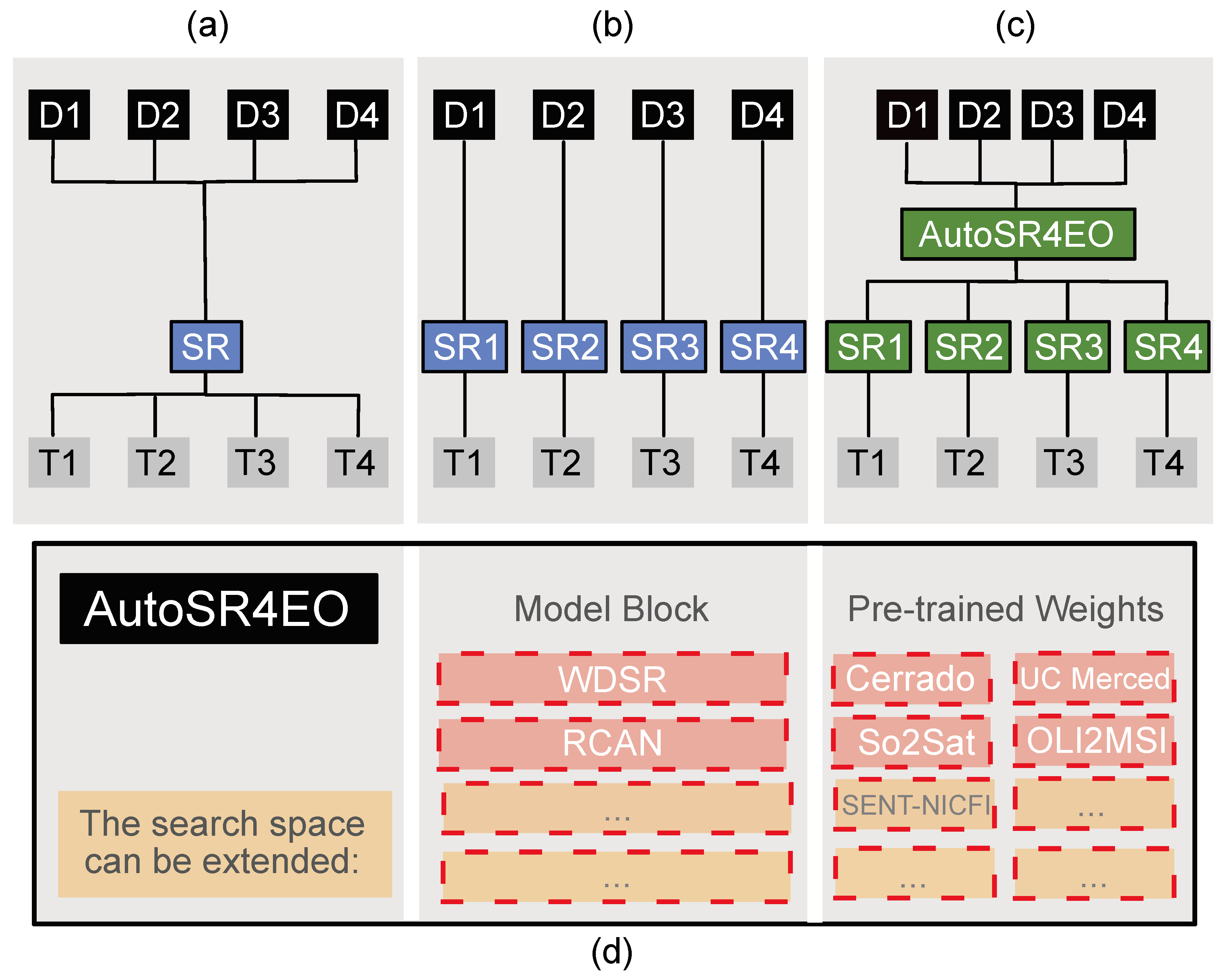
- We propose AutoSR4EO, the first AutoML system for SR for EO, by designing a customised search space based on state-of-the-art research in SR;
- We further propose to use pre-trained weights generated from EO datasets in AutoSR4EO to facilitate knowledge transfer and speed up the training of SR methods for EO tasks;
- We introduce a vanilla baseline AutoML system for SR, dubbed AutoSRCNN, based on existing NAS search spaces consisting exclusively of convolutional layers, which is useful as a lower-bound baseline for comparison to future AutoML approaches for SR;
- We evaluate the performance of AutoSR4EO on four EO datasets in terms of peak signal-to-noise ratio (PSNR) and structural similarity index (SSIM) and compare our methods to four state-of-the-art SR methods and AutoSRCNN;
2. Related Work
2.1. Super-Resolution
2.2. AutoML for EO Tasks
NAS Systems for SR
2.3. Relevance of Our Work
3. Materials and Methods
3.1. Methods
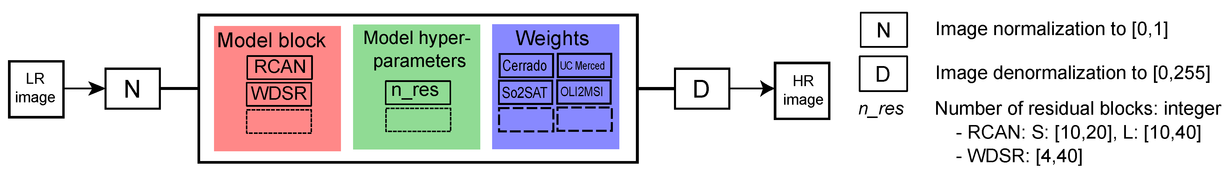
3.1.1. Search Space
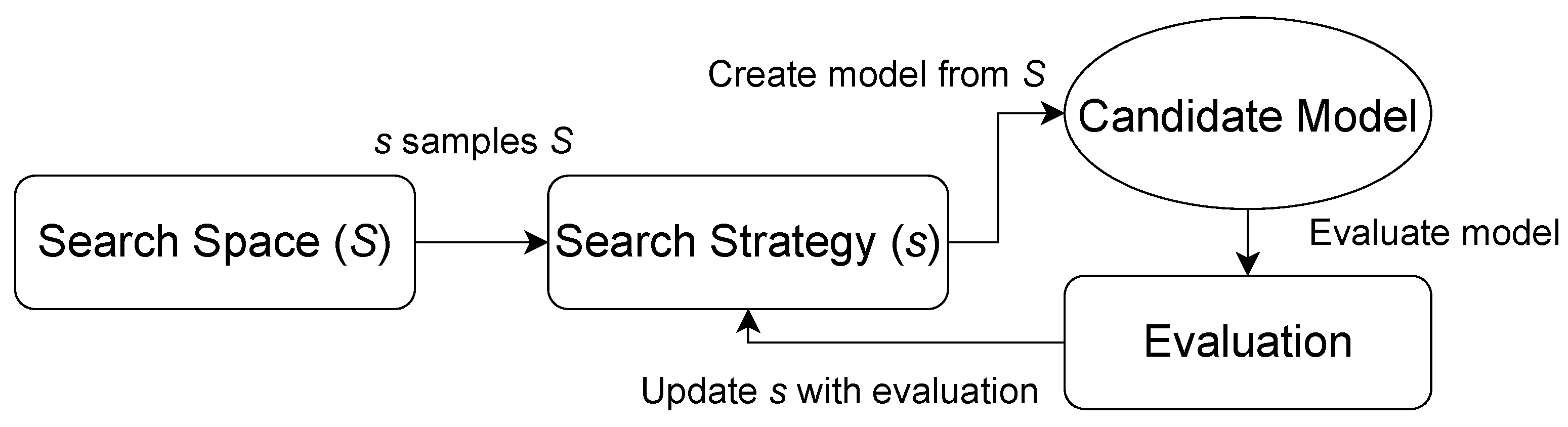
3.1.2. Search Strategy
3.2. Data
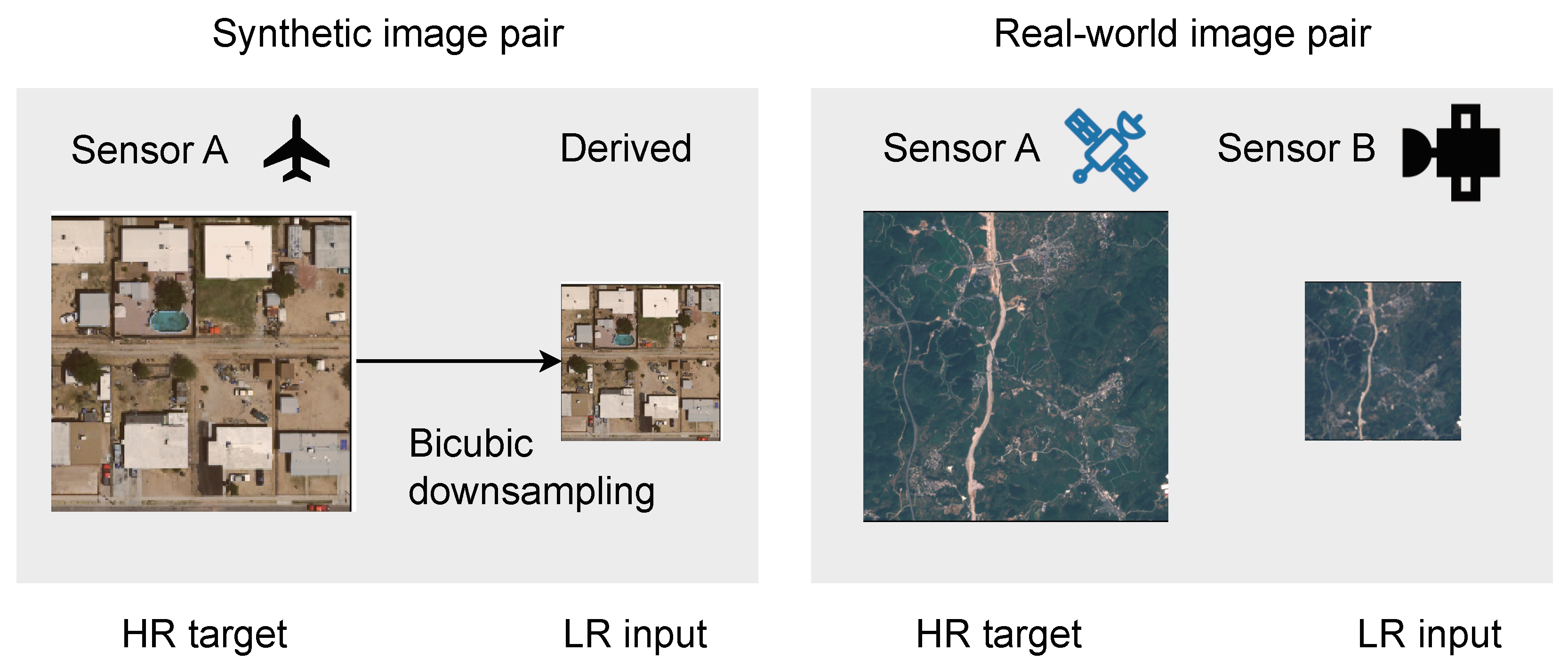
3.2.1. Synthetic Datasets
- UC Merced [16], which is a dataset for land use image classification containing 21 different classes of terrain in the United States;
- So2Sat [62], which is a dataset comprising images of 42 different cities across different continents. The RGB subset of So2Sat consists of Sentinel-2 images. We used this dataset exclusively to generate the pre-trained weights because the large size of the dataset made it infeasible to evaluate AutoSR4EO on this dataset using the current experimental setup;
- Cerrado-Savanna [82], which consists of images of Brazil’s Serra do Cipó region and has a wide variety of vegetation and high variations between classes.
3.2.2. Real-World Datasets
- OLI2MSI, proposed by Wang et al. [17], which consists of low-resolution images taken by Landsat-8 and Sentinel-2 of a region in Southwest China and contains 10,650 training pairs;
- SENT-NICFI, which is a novel SR dataset we constructed using images from Sentinel-2 and Planetscope that were taken in June 2021. The Planetscope images are part of the NICFI programme. We selected images of countries around the equator, covering an area of about 45 million square kilometres. We selected high-resolution (HR) images from five scenes from each of the following ecosystems from countries on the African continent: urban, desert, forest, savanna, agriculture and miscellaneous (i.e., outside of the previous categories). The low-resolution (LR) images were Sentinel-2 images from around the same month, producing 12,000 training pairs. We aligned the HR image colours to the LR images via histogram matching. We provide code for the reconstruction of this dataset.
3.3. Experiments
3.3.1. Baselines
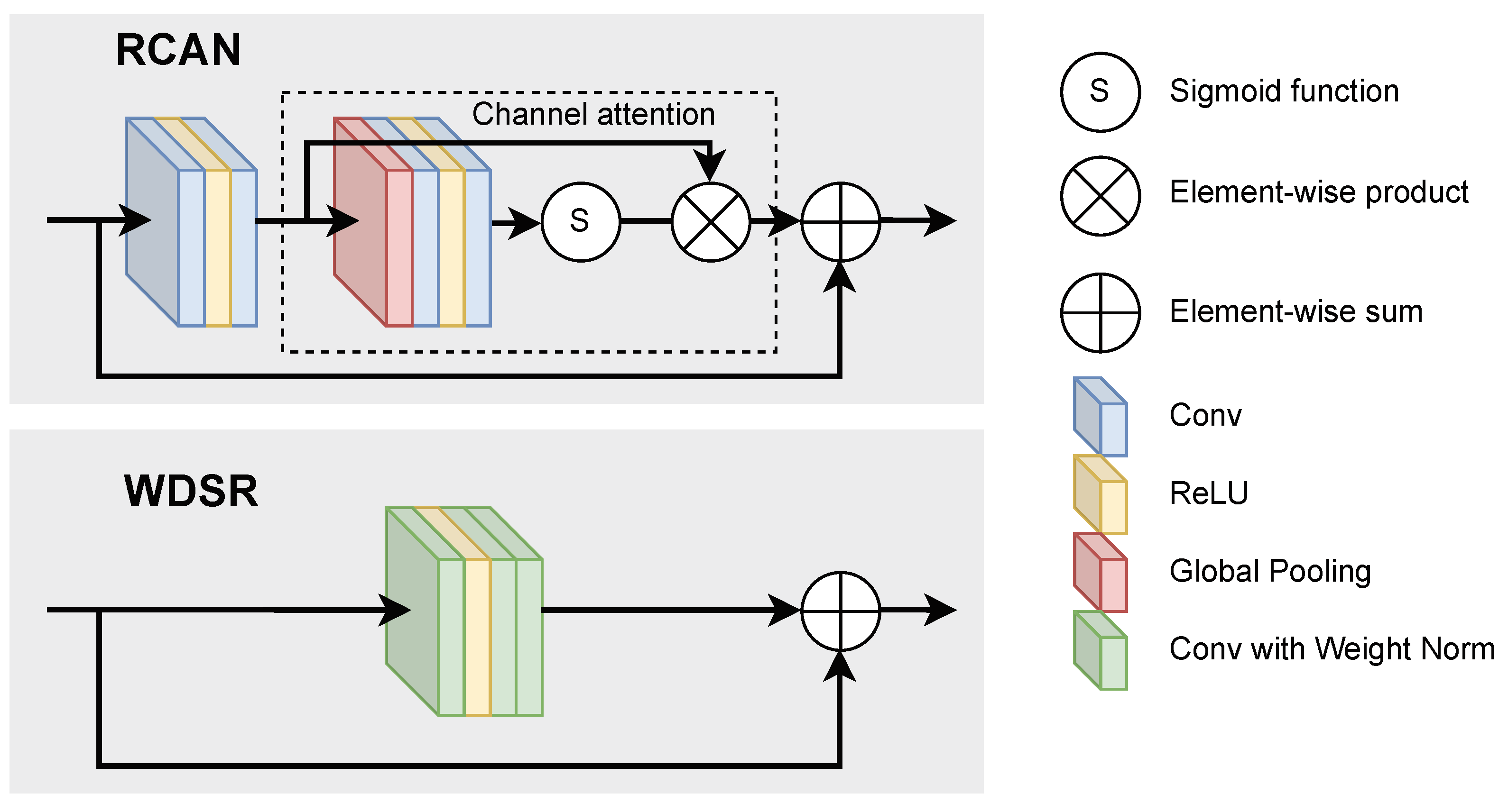
- RCAN [30], which introduces channel attention modules that give more weight to informative features. The network consists of stacked residual groups, with an upscaling module at the end of the residual stack after merging the two branches. We used the Keras implementation of RCAN, made available by Hieubkset (https://github.com/hieubkset/Keras-Image-SR, accessed on 28 June 2022);
- WDSR [28], which is a residual approach, like RCAN, but the residual blocks lack the channel attention mechanism. The two branches are merged after upsampling on each of them. Convolutions with weight normalisation replace all convolutional layers. We used the Keras code for the WDSR model released by Krasser (https://github.com/krasserm/super-resolution, accessed on 28 June 2022);
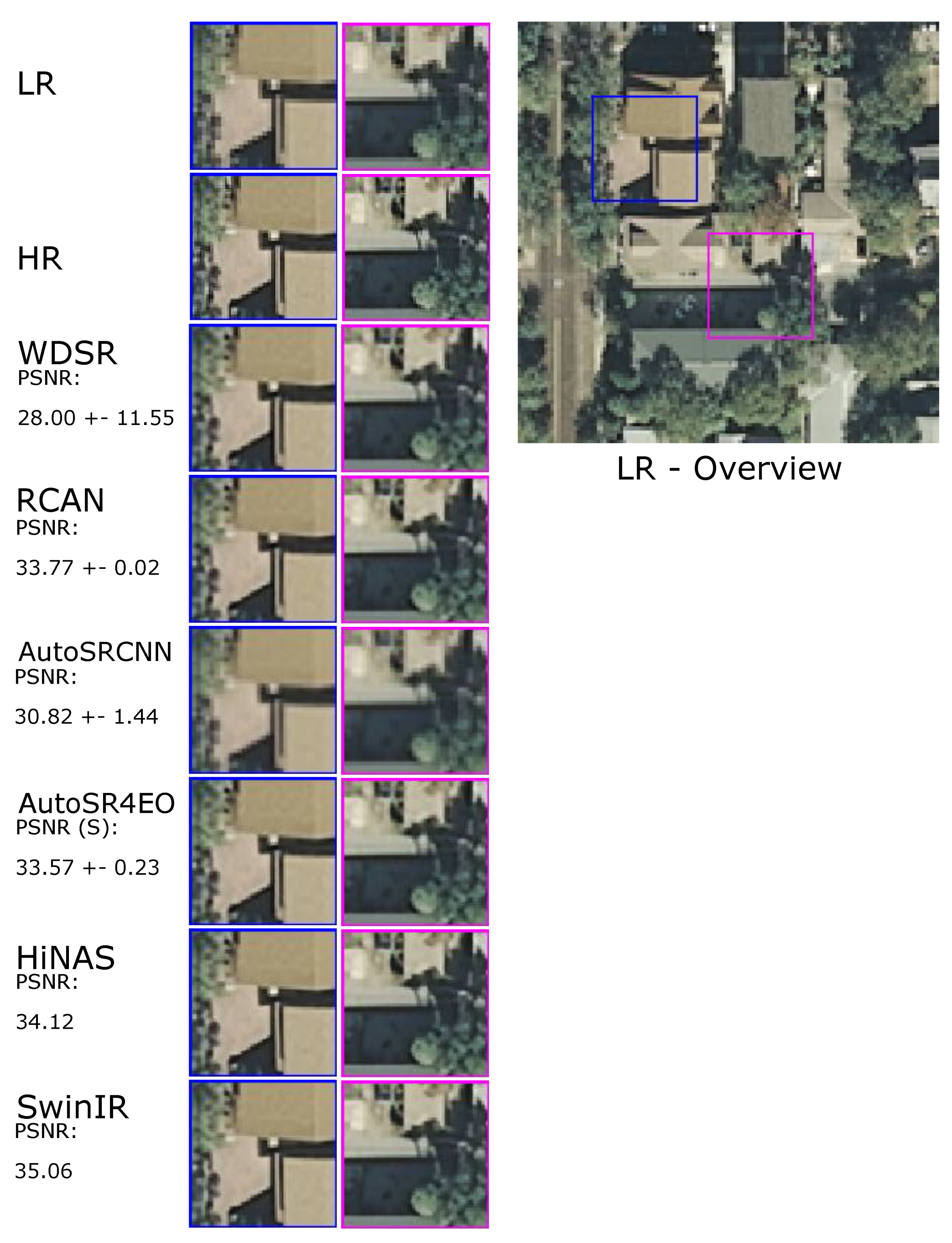
- SwinIR [9], which is a state-of-the-art adaptation of the Swin Transformer [49] for image reconstruction and super-resolution. We used the DIV2K and Flickr2K pre-trained models (https://github.com/JingyunLiang/SwinIR, accessed on 1 September 2023). We followed the original work and selected the “Medium” configuration, which is comparable in complexity to RCAN, with a patch size of 64 and a window size of 8. We directly inferred on our test sets (as defined in Section 3.2, as in the original work, but with natural image test sets (Set5 [72], BSD100 [72], Set14 [73] Urban100 [74] and Manga109 [84]);
- HiNAS [69], which is a state-of-the-art NAS framework for super-resolution and image denoising. It is computationally efficient due to its gradient-based search and architecture sharing between layers. We searched and trained the best networks for the upscaling factors of 2 and 3, following the original work. The evaluation was the same as for SwinIR;
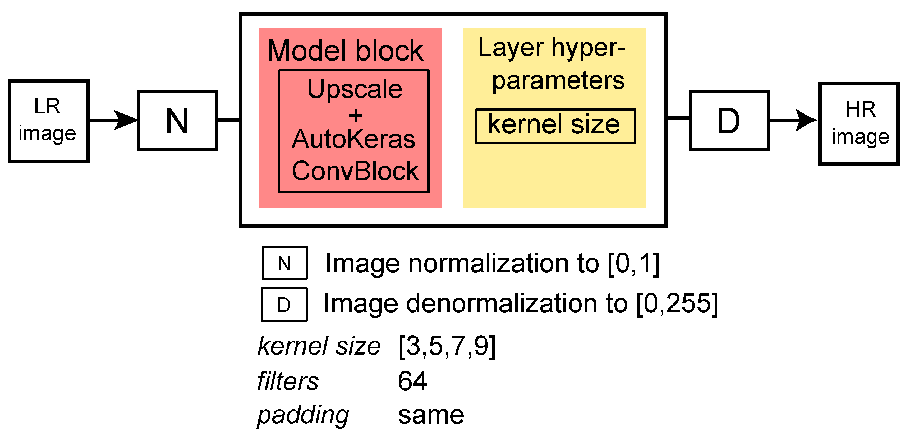
- AutoSRCNN, which is an AutoML SR approach inspired by SRCNN [25]. We implemented AutoSRCNN exclusively with convolutional layers, without residual connections, pre-trained weights or specialised blocks. The search space (shown in Figure 5) is much smaller than that of AutoSR4EO; thus, it served as a control to ensure that a more extensive search space is beneficial for solving the problem of SISR for EO images. AutoSRCNN found networks comparable to SRCNN, which are less complex than the state-of-the-art alternatives. As such, AutoSRCNN served as a vanilla baseline to AutoSR4EO.
3.3.2. Training Details
3.3.3. Evaluation
3.3.4. Experimental Setup
4. Results
4.1. Performance Evaluation
Additional Trials
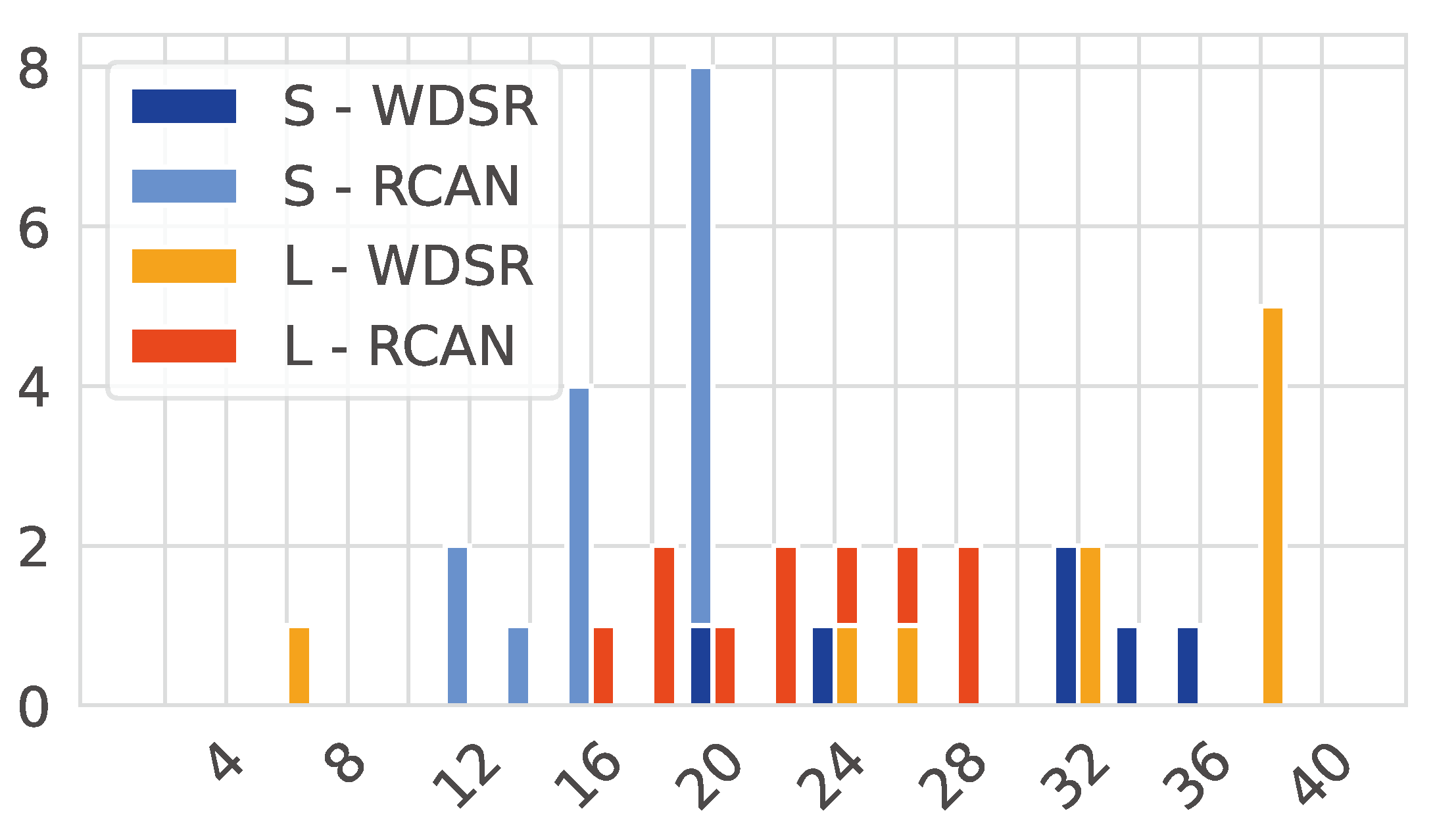
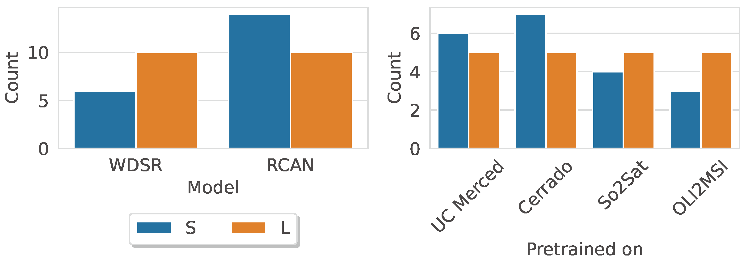
4.2. Search Space Analysis
5. Discussion
5.1. Interpretation of the Findings
5.1.1. Performance Evaluation
5.1.2. Search Space Analysis
5.2. Limitations
5.2.1. Search Space
5.2.2. Real-World Datasets and SENT-NICFI
5.2.3. Evaluation Metrics and Baselines
5.3. Future Work
6. Conclusions
Author Contributions
Funding
Data Availability Statement
Acknowledgments
Conflicts of Interest
Abbreviations
| AutoML | Automated machine learning |
| EO | Earth observation |
| ML | Machine learning |
| NAS | Neural architecture search |
| PSNR | Peak signal-to-noise ratio |
| SISR | Single-image super-resolution |
| SOTA | State-of-the-art |
| SSIM | Structural similarity index measure |
| SR | Super-resolution |
References
- He, D.; Shi, Q.; Liu, X.; Zhong, Y.; Xia, G.; Zhang, L. Generating annual high resolution land cover products for 28 metropolises in China based on a deep super-resolution mapping network using Landsat imagery. GIScience Remote Sens. 2022, 59, 2036–2067. [Google Scholar] [CrossRef]
- Synthiya Vinothini, D.; Sathyabama, B.; Karthikeyan, S. Super Resolution Mapping of Trees for Urban Forest Monitoring in Madurai City Using Remote Sensing. In Proceedings of the Computer Vision, Graphics, and Image Processing, Guwahati, India, 19 December 2016; Mukherjee, S., Mukherjee, S., Mukherjee, D.P., Sivaswamy, J., Awate, S., Setlur, S., Namboodiri, A.M., Chaudhury, S., Eds.; Springer: Cham, Switzerland, 2017; pp. 88–96. [Google Scholar] [CrossRef]
- Garcia-Pedrero, A.; Gonzalo-Martín, C.; Lillo-Saavedra, M.; Rodríguez-Esparragón, D. The Outlining of Agricultural Plots Based on Spatiotemporal Consensus Segmentation. Remote Sens. 2018, 10, 1991. [Google Scholar] [CrossRef]
- Wang, P.; Zhang, G.; Leung, H. Improving Super-Resolution Flood Inundation Mapping for Multispectral Remote Sensing Image by Supplying More Spectral Information. IEEE Geosci. Remote Sens. Lett. 2019, 16, 771–775. [Google Scholar] [CrossRef]
- Shermeyer, J.; Van Etten, A. The Effects of Super-Resolution on Object Detection Performance in Satellite Imagery. In Proceedings of the IEEE/CVF Conference on Computer Vision and Pattern Recognition (CVPR) Workshops, Long Beach, CA, USA, 15–20 June 2019. [Google Scholar] [CrossRef]
- Zou, F.; Xiao, W.; Ji, W.; He, K.; Yang, Z.; Song, J.; Zhou, H.; Li, K. Arbitrary-oriented object detection via dense feature fusion and attention model for remote sensing super-resolution image. Neural Comput. Appl. 2020, 32, 14549–14562. [Google Scholar] [CrossRef]
- Haris, M.; Shakhnarovich, G.; Ukita, N. Task-driven super resolution: Object detection in low-resolution images. In Proceedings of the International Conference on Neural Information Processing, Killarney, Ireland, 12–17 July 2015; Springer: Berlin/Heidelberg, Germany, 2021; pp. 387–395. [Google Scholar] [CrossRef]
- Michel, J.; Vinasco-Salinas, J.; Inglada, J.; Hagolle, O. SEN2VENUS, a Dataset for the Training of Sentinel-2 Super-Resolution Algorithms. Data 2022, 7, 96. [Google Scholar] [CrossRef]
- Liang, J.; Cao, J.; Sun, G.; Zhang, K.; Gool, L.V.; Timofte, R. SwinIR: Image Restoration Using Swin Transformer. In Proceedings of the 2021 IEEE/CVF International Conference on Computer Vision Workshops (ICCVW), Los Alamitos, CA, USA, 17–21 October 2021; pp. 1833–1844. [Google Scholar] [CrossRef]
- Ahn, J.Y.; Cho, N.I. Neural Architecture Search for Image Super-Resolution Using Densely Constructed Search Space: DeCoNAS. In Proceedings of the 2020 25th International Conference on Pattern Recognition (ICPR), Milan, Italy, 10–15 January 2021; pp. 4829–4836. [Google Scholar] [CrossRef]
- Ahn, N.; Kang, B.; Sohn, K.A. Fast, accurate, and lightweight super-resolution with cascading residual network. In Proceedings of the European Conference on Computer Vision (ECCV), Munich, Germany, 8–14 September 2018; pp. 252–268. [Google Scholar] [CrossRef]
- Ran, Q.; Xu, X.; Zhao, S.; Li, W.; Du, Q. Remote sensing images super-resolution with deep convolution networks. Multimed. Tools Appl. 2020, 79, 8985–9001. [Google Scholar] [CrossRef]
- Xu, W.; XU, G.; Wang, Y.; Sun, X.; Lin, D.; WU, Y. High Quality Remote Sensing Image Super-Resolution Using Deep Memory Connected Network. In Proceedings of the IGARSS 2018–2018 IEEE International Geoscience and Remote Sensing Symposium, Valencia, Spain, 22–27 July 2018; pp. 8889–8892. [Google Scholar] [CrossRef]
- Köhler, T.; Bätz, M.; Naderi, F.; Kaup, A.; Maier, A.; Riess, C. Toward Bridging the Simulated-to-Real Gap: Benchmarking Super-Resolution on Real Data. IEEE Trans. Pattern Anal. Mach. Intell. 2020, 42, 2944–2959. [Google Scholar] [CrossRef]
- Elsken, T.; Metzen, J.H.; Hutter, F. Neural Architecture Search: A Survey. J. Mach. Learn. Res. 2019, 20, 1997–2017. [Google Scholar]
- Yang, Y.; Newsam, S. Bag-of-Visual-Words and Spatial Extensions for Land-Use Classification. In Proceedings of the 18th SIGSPATIAL International Conference on Advances in Geographic Information Systems (GIS ’10), San Jose, CA, USA, 2–5 November 2010; pp. 270–279. [Google Scholar] [CrossRef]
- Wang, J.; Gao, K.; Zhang, Z.; Ni, C.; Hu, Z.; Chen, D.; Wu, Q. Multisensor Remote Sensing Imagery Super-Resolution with Conditional GAN. J. Remote Sens. 2021, 2021. [Google Scholar] [CrossRef]
- European Space Agency. Orbit—Sentinel 2-Mission-Sentinel Online-Sentinel Online. Available online: https://sentinel.esa.int/web/sentinel/missions/sentinel-2/satellite-description/orbit (accessed on 16 May 2022).
- Norway’s International Climate and Forest Initiative (NICFI). 2022. Available online: https://www.nicfi.no/ (accessed on 28 June 2022).
- Gu, S.; Sang, N.; Ma, F. Fast image super resolution via local regression. In Proceedings of the 21st International Conference on Pattern Recognition (ICPR2012), Tskuba Science City, Japan, 11–15 November 2012; pp. 3128–3131. [Google Scholar]
- Timofte, R.; De, V.; Gool, L.V. Anchored Neighborhood Regression for Fast Example-Based Super-Resolution. In Proceedings of the 2013 IEEE International Conference on Computer Vision, Sydney, Australia, 1–8 December 2013; pp. 1920–1927. [Google Scholar] [CrossRef]
- Timofte, R.; De Smet, V.; Van Gool, L. A+: Adjusted anchored neighborhood regression for fast super-resolution. In Computer Vision–ACCV 2014, Revised Selected Papers, Part IV 12, Proceedings of the 12th Asian Conference on Computer Vision, Singapore, 1–5 November 2014; Springer: Berlin/Heidelberg, Germany, 2015; pp. 111–126. [Google Scholar] [CrossRef]
- Michaeli, T.; Irani, M. Nonparametric Blind Super-resolution. In Proceedings of the 2013 IEEE International Conference on Computer Vision, Sydney, Australia, 1–8 December 2013; pp. 945–952. [Google Scholar] [CrossRef]
- Moser, B.B.; Raue, F.; Frolov, S.; Palacio, S.; Hees, J.; Dengel, A. Hitchhiker’s Guide to Super-Resolution: Introduction and Recent Advances. IEEE Trans. Pattern Anal. Mach. Intell. 2023, 45, 1–21. [Google Scholar] [CrossRef]
- Dong, C.; Loy, C.C.; He, K.; Tang, X. Learning a Deep Convolutional Network for Image Super-Resolution. In Proceedings of the Lecture Notes in Computer Science (including Subseries Lecture Notes in Artificial Intelligence and Lecture Notes in Bioinformatics), Zurich, Switzerland, 6–12 September 2014; 8692 LNCS. pp. 184–199. [Google Scholar] [CrossRef]
- Kim, J.; Lee, J.K.; Lee, K.M. Accurate image super-resolution using very deep convolutional networks. In Proceedings of the IEEE Conference on Computer Vision and Pattern Recognition, Las Vegas, NV, USA, 26 June–1 July 2016; pp. 1646–1654. [Google Scholar] [CrossRef]
- Lim, B.; Son, S.; Kim, H.; Nah, S.; Mu Lee, K. Enhanced deep residual networks for single image super-resolution. In Proceedings of the IEEE Conference on Computer Vision and Pattern Recognition Workshops, Honolulu, HI, USA, 21–26 July 2017; pp. 136–144. [Google Scholar] [CrossRef]
- Fan, Y.; Yu, J.; Huang, T.S. Wide-activated deep residual networks based restoration for bpg-compressed images. In Proceedings of the IEEE Conference on Computer Vision and Pattern Recognition Workshops, Salt Lake City, UT, USA, 18–22 June 2018; pp. 2621–2624. [Google Scholar]
- Li, J. Multi-scale Residual Network for Image Super-Resolution. In Proceedings of the European Conference on Computer Vision (ECCV), Munich, Germany, 8–14 September 2018. [Google Scholar] [CrossRef]
- Zhang, Y.; Li, K.; Li, K.; Wang, L.; Zhong, B.; Fu, Y. Image super-resolution using very deep residual channel attention networks. In Proceedings of the European Conference on Computer Vision (ECCV), Munich, Germany, 8–14 September 2018; pp. 286–301. [Google Scholar] [CrossRef]
- Wang, C.; Li, Z.; Shi, J. Lightweight Image Super-Resolution with Adaptive Weighted Learning Network. arXiv 2019. [Google Scholar] [CrossRef]
- Liu, Z.S.; Wang, L.W.; Li, C.T.; Siu, W.C. Hierarchical Back Projection Network for Image Super-Resolution. In Proceedings of the IEEE/CVF Conference on Computer Vision and Pattern Recognition Workshops, Long Beach, CA, USA, 16–20 June 2019. [Google Scholar] [CrossRef]
- Ledig, C.; Theis, L.; Huszár, F.; Caballero, J.; Cunningham, A.; Acosta, A.; Aitken, A.; Tejani, A.; Totz, J.; Wang, Z.; et al. Photo-realistic single image super-resolution using a generative adversarial network. In Proceedings of the IEEE Conference on Computer Vision and Pattern Recognition, Honolulu, HI, USA, 21–26 July 2017; pp. 4681–4690. [Google Scholar] [CrossRef]
- Jiang, K.; Wang, Z.; Yi, P.; Wang, G.; Lu, T.; Jiang, J. Edge-enhanced GAN for remote sensing image superresolution. IEEE Trans. Geosci. Remote Sens. 2019, 57, 5799–5812. [Google Scholar] [CrossRef]
- Wang, X.; Yu, K.; Wu, S.; Gu, J.; Liu, Y.; Dong, C.; Qiao, Y.; Loy, C.C. ESRGAN: Enhanced Super-Resolution Generative Adversarial Networks. In ECCV 2018 Workshops, Proceedings of the Computer Vision, Munich, Germany, 8–14 September 2018; Leal-Taixé, L., Roth, S., Eds.; Springer: Cham, Switzerland, 2019; pp. 63–79. [Google Scholar]
- Rakotonirina, N.C.; Rasoanaivo, A. ESRGAN+: Further Improving Enhanced Super-Resolution Generative Adversarial Network. In Proceedings of the ICASSP 2020, 2020 IEEE International Conference on Acoustics, Speech and Signal Processing (ICASSP), Barcelona, Spain, 4–8 May 2020; pp. 3637–3641. [Google Scholar] [CrossRef]
- Sajjadi, M.S.M.; Schölkopf, B.; Hirsch, M. EnhanceNet: Single Image Super-Resolution Through Automated Texture Synthesis. In Proceedings of the IEEE International Conference on Computer Vision (ICCV) Venice, Paris, Italy, 22–29 October 2017. [Google Scholar] [CrossRef]
- Tao, Y.; Muller, J.P.; Hamedianfar, A.; Shafri, H. Super-Resolution Restoration of Spaceborne Ultra-High-Resolution Images Using the UCL OpTiGAN System. Remote Sens. 2021, 13, 2269. [Google Scholar] [CrossRef]
- Jia, S.; Wang, Z.; Li, Q.; Jia, X.; Xu, M. Multiattention Generative Adversarial Network for Remote Sensing Image Super-Resolution. IEEE Trans. Geosci. Remote Sens. 2022, 60, 1–15. [Google Scholar] [CrossRef]
- Xu, Y.; Luo, W.; Hu, A.; Xie, Z.; Xie, X.; Tao, L. TE-SAGAN: An Improved Generative Adversarial Network for Remote Sensing Super-Resolution Images. Remote Sens. 2022, 14, 2425. [Google Scholar] [CrossRef]
- Guo, M.; Zhang, Z.; Liu, H.; Huang, Y. NDSRGAN: A Novel Dense Generative Adversarial Network for Real Aerial Imagery Super-Resolution Reconstruction. Remote Sens. 2022, 14, 1574. [Google Scholar] [CrossRef]
- Singla, K.; Pandey, R.; Ghanekar, U. A review on Single Image Super Resolution techniques using generative adversarial network. Optik 2022, 266, 169607. [Google Scholar] [CrossRef]
- Gao, C.; Chen, Y.; Liu, S.; Tan, Z.; Yan, S. AdversarialNAS: Adversarial Neural Architecture Search for GANs. In Proceedings of the IEEE/CVF Conference on Computer Vision and Pattern Recognition, Seattle, WA, USA, 13–19 June 2020. [Google Scholar] [CrossRef]
- Gong, X.; Chang, S.; Jiang, Y.; Wang, Z. AutoGAN: Neural Architecture Search for Generative Adversarial Networks. In Proceedings of the 2019 IEEE/CVF International Conference on Computer Vision (ICCV), Los Alamitos, CA, USA, 27 October–2 November 2019; pp. 3223–3233. [Google Scholar] [CrossRef]
- Ganepola, V.V.V.; Wirasingha, T. Automating generative adversarial networks using neural architecture search: A review. In Proceedings of the 2021 International Conference on Emerging Smart Computing and Informatics, ESCI 2021, Pune, India, 5–7 March 2021; pp. 577–582. [Google Scholar] [CrossRef]
- Dosovitskiy, A.; Beyer, L.; Kolesnikov, A.; Weissenborn, D.; Zhai, X.; Unterthiner, T.; Dehghani, M.; Minderer, M.; Heigold, G.; Gelly, S.; et al. An Image is Worth 16x16 Words: Transformers for Image Recognition at Scale. arXiv 2020, arXiv:2010.11929. [Google Scholar]
- Wu, H.; Xiao, B.; Codella, N.; Liu, M.; Dai, X.; Yuan, L.; Zhang, L. CvT: Introducing Convolutions to Vision Transformers. In Proceedings of the 2021 IEEE/CVF International Conference on Computer Vision (ICCV), Los Alamitos, CA, USA, 11–17 October 2021; pp. 22–31. [Google Scholar] [CrossRef]
- Touvron, H.; Cord, M.; Douze, M.; Massa, F.; Sablayrolles, A.; Jegou, H. Training data-efficient image transformers; distillation through attention. In Proceedings of Machine Learning, Proceedings of the 38th International Conference on Machine Learning, Online, 18–24 July 2021; Meila, M., Zhang, T., Eds.; Springer: Berlin/Heidelberg, Germany, 2018; Volume 139, pp. 10347–10357. [Google Scholar]
- Liu, Z.; Lin, Y.; Cao, Y.; Hu, H.; Wei, Y.; Zhang, Z.; Lin, S.; Guo, B. Swin Transformer: Hierarchical Vision Transformer using Shifted Windows. In Proceedings of the 2021 IEEE/CVF International Conference on Computer Vision (ICCV), Los Alamitos, CA, USA, 11–17 October 2021; pp. 9992–10002. [Google Scholar] [CrossRef]
- Han, L.; Zhao, Y.; Lv, H.; Zhang, Y.; Liu, H.; Bi, G.; Han, Q. Enhancing Remote Sensing Image Super-Resolution with Efficient Hybrid Conditional Diffusion Model. Remote Sens. 2023, 15, 3452. [Google Scholar] [CrossRef]
- Wu, H.; Ni, N.; Wang, S.; Zhang, L. Conditional Stochastic Normalizing Flows for Blind Super-Resolution of Remote Sensing Images. IEEE Trans. Geosci. Remote Sens. 2023, 61, 1–16. [Google Scholar] [CrossRef]
- Ali, A.M.; Benjdira, B.; Koubaa, A.; Boulila, W.; El-Shafai, W. TESR: Two-Stage Approach for Enhancement and Super-Resolution of Remote Sensing Images. Remote Sens. 2023, 15, 2346. [Google Scholar] [CrossRef]
- Feurer, M.; Klein, A.; Eggensperger, K.; Springenberg, J.T.; Blum, M.; Hutter, F. Efficient and Robust Automated Machine Learning. In Proceedings of the 28th International Conference on Neural Information Processing Systems—Volume 2 (NIPS’15), Cambridge, MA, USA, Montreal, QC, Canada, 7–12 December 2015; pp. 2755–2763. [Google Scholar]
- Feurer, M.; Eggensperger, K.; Falkner, S.; Lindauer, M.; Hutter, F. Auto-Sklearn 2.0: Hands-Free AutoML via Meta-Learning. J. Mach. Learn. Res. 2022, 23, 1–61. [Google Scholar]
- Erickson, N.; Mueller, J.; Shirkov, A.; Zhang, H.; Larroy, P.; Li, M.; Smola, A. AutoGluon-Tabular: Robust and Accurate AutoML for Structured Data. arXiv 2020, arXiv:2003.06505. [Google Scholar]
- Wang, C.; Wu, Q.; Weimer, M.; Zhu, E. Flaml: A fast and lightweight automl library. Proc. Mach. Learn. Syst. 2021, 3, 434–447. [Google Scholar]
- Jin, H.; Song, Q.; Hu, X. Auto-Keras: An Efficient Neural Architecture Search System. In Proceedings of the 25th ACM SIGKDD International Conference on Knowledge Discovery & Data Mining (KDD ’19), New York, NY, USA, 4–18 August 2019; pp. 1946–1956. [Google Scholar] [CrossRef]
- Zimmer, L.; Lindauer, M.; Hutter, F. Auto-Pytorch: Multi-Fidelity MetaLearning for Efficient and Robust AutoDL. IEEE Trans. Pattern Anal. Mach. Intell. 2021, 43, 3079–3090. [Google Scholar] [CrossRef] [PubMed]
- de Sá, N.C.; Baratchi, M.; Buitenhuis, V.; Cornelissen, P.; van Bodegom, P.M. AutoML for estimating grass height from ETM+/OLI data from field measurements at a nature reserve. GIScience Remote Sens. 2022, 59, 2164–2183. [Google Scholar] [CrossRef]
- Zheng, Z.; Fiore, A.M.; Westervelt, D.M.; Milly, G.P.; Goldsmith, J.; Karambelas, A.; Curci, G.; Randles, C.A.; Paiva, A.R.; Wang, C.; et al. Automated Machine Learning to Evaluate the Information Content of Tropospheric Trace Gas Columns for Fine Particle Estimates Over India: A Modeling Testbed. J. Adv. Model. Earth Syst. 2023, 15, e2022MS003099. [Google Scholar] [CrossRef]
- Helber, P.; Bischke, B.; Dengel, A.; Borth, D. EuroSAT: A Novel Dataset and Deep Learning Benchmark for Land Use and Land Cover Classification. IEEE J. Sel. Top. Appl. Earth Obs. Remote Sens. 2019, 12, 2217–2226. [Google Scholar] [CrossRef]
- Zhu, X.X.; Hu, J.; Qiu, C.; Shi, Y.; Kang, J.; Mou, L.; Bagheri, H.; Haberle, M.; Hua, Y.; Huang, R.; et al. So2Sat LCZ42: A Benchmark Data Set for the Classification of Global Local Climate Zones [Software and Data Sets]. IEEE Geosci. Remote Sens. Mag. 2020, 8, 76–89. [Google Scholar] [CrossRef]
- Cheng, G.; Han, J.; Lu, X. Remote Sensing Image Scene Classification: Benchmark and State of the Art. Proc. IEEE 2017, 105, 1865–1883. [Google Scholar] [CrossRef]
- Palacios Salinas, N.R.; Baratchi, M.; van Rijn, J.N.; Vollrath, A. Automated Machine Learning for Satellite Data: Integrating Remote Sensing Pre-Trained Models into AutoML Systems. In Proceedings of the Machine Learning and Knowledge Discovery in Databases. Applied Data Science Track: European Conference, ECML PKDD 2021, Bilbao, Spain, 13–17 September 2021; p. C1. [Google Scholar] [CrossRef]
- Polonskaia, I.S.; Aliev, I.R.; Nikitin, N.O. Automated Evolutionary Design of CNN Classifiers for Object Recognition on Satellite Images. Procedia Comput. Sci. 2021, 193, 210–219. [Google Scholar] [CrossRef]
- Chu, X.; Zhang, B.; Xu, R. Multi-Objective Reinforced Evolution in Mobile Neural Architecture Search. In Proceedings Part IV, Proceedings of the Computer Vision—ECCV 2020 Workshops, Glasgow, UK, 23–28 August 2020; Springer: Cham, Switzerland, 2020; pp. 99–113. [Google Scholar] [CrossRef]
- Chu, X.; Zhang, B.; Ma, H.; Xu, R.; Li, Q. Fast, Accurate and Lightweight Super-Resolution with Neural Architecture Search. In Proceedings of the 2020 25th International Conference on Pattern Recognition (ICPR), Taichung, Taiwan, 18–21 July 2021; pp. 59–64. [Google Scholar] [CrossRef]
- Ahn, J.Y.; Cho, N.I. Multi-Branch Neural Architecture Search for Lightweight Image Super-Resolution. IEEE Access 2021, 9, 153633–153646. [Google Scholar] [CrossRef]
- Zhang, H.; Li, Y.; Chen, H.; Shen, C. Memory-Efficient Hierarchical Neural Architecture Search for Image Denoising. In Proceedings of the 2020 IEEE/CVF Conference on Computer Vision and Pattern Recognition (CVPR), Los Alamitos, CA, USA, 12 June 2020; pp. 3654–3663. [Google Scholar] [CrossRef]
- Chen, Y.C.; Gao, C.; Robb, E.; Huang, J.B. NAS-DIP: Learning Deep Image Prior with Neural Architecture Search. In Proceedings of the Computer Vision—ECCV 2020; Vedaldi, A., Bischof, H., Brox, T., Frahm, J.M., Eds.; Springer: Cham, Switzerland, 2020; pp. 442–459. [Google Scholar] [CrossRef]
- Agustsson, E.; Timofte, R. NTIRE 2017 Challenge on Single Image Super-Resolution: Dataset and Study. In Proceedings of the 2017 IEEE Conference on Computer Vision and Pattern Recognition Workshops (CVPRW), Honolulu, HI, USA, 21–26 July 2017; pp. 1122–1131. [Google Scholar] [CrossRef]
- Bevilacqua, M.; Roumy, A.; Guillemot, C.; Alberi-Morel, M.L. Low-complexity single-image super-resolution based on nonnegative neighbor embedding. In Proceedings of the 23rd British Machine Vision Conference (BMVC), Surrey, UK, 3–7 September 2012. [Google Scholar]
- Zeyde, R.; Elad, M.; Protter, M. On single image scale-up using sparse-representations. In Proceedings of the International Conference on Curves and Surfaces, Avignon, France, 24–30 June 2010; pp. 711–730. [Google Scholar] [CrossRef]
- Huang, J.B.; Singh, A.; Ahuja, N. Single image super-resolution from transformed self-exemplars. In Proceedings of the 2015 IEEE Conference on Computer Vision and Pattern Recognition (CVPR), Boston, MA, USA, 7–12 June 2015; pp. 5197–5206. [Google Scholar] [CrossRef]
- Deng, J.; Dong, W.; Socher, R.; Li, L.J.; Li, K.; Fei-Fei, L. ImageNet: A large-scale hierarchical image database. In Proceedings of the 2009 IEEE Conference on Computer Vision and Pattern Recognition, Miami, FL, USA, 20–25 June 2009; pp. 248–255. [Google Scholar] [CrossRef]
- He, K.; Zhang, X.; Ren, S.; Sun, J. Deep residual learning for image recognition. In Proceedings of the IEEE Conference on Computer Vision and Pattern Recognition, Las Vegas, NV, USA, 26 June–1 July 2016; pp. 770–778. [Google Scholar] [CrossRef]
- Wang, Z.; Chen, J.; Hoi, S.C. Deep Learning for Image Super-Resolution: A Survey. IEEE Trans. Pattern Anal. Mach. Intell. 2021, 43, 3365–3387. [Google Scholar] [CrossRef] [PubMed]
- Timofte, R.; Gu, S.; Wu, J.; Van Gool, L.; Zhang, L.; Yang, M.H.; Haris, M.; Shakhnarovich, G.; Ukita, N.; Hu, S.; et al. NTIRE 2018 Challenge on Single Image Super-Resolution: Methods and Results. In Proceedings of the 2018 IEEE/CVF Conference on Computer Vision and Pattern Recognition Workshops (CVPRW), Salt Lake City, UT, USA, 18–22 June 2018; pp. 965–96511. [Google Scholar] [CrossRef]
- Ha, V.K.; Ren, J.; Xu, X.; Zhao, S.; Xie, G.; Vargas, V.M. Deep learning based single image super-resolution: A survey. Int. J. Autom. Comput. 2019, 16, 413–426. [Google Scholar] [CrossRef]
- Li, J.; Pei, Z.; Zeng, T. From Beginner to Master: A Survey for Deep Learning-based Single-Image Super-Resolution. arXiv 2021, arXiv:2109.14335. [Google Scholar]
- Microsoft. Neural Network Intelligence; McGraw-Hill, Inc.: New York, NY, USA, 2021. [Google Scholar]
- Nogueira, K.; Dos Santos, J.A.; Fornazari, T.; Freire Silva, T.S.; Morellato, L.P.; Torres, R.D.S. Towards vegetation species discrimination by using data-driven descriptors. In Proceedings of the 2016 9th IAPR Workshop on Pattern Recogniton in Remote Sensing (PRRS), Cancun, Mexico, 4 December 2016; pp. 1–6. [Google Scholar] [CrossRef]
- Razzak, M.T.; Mateo-Garcia, G.; Lecuyer, G.; Gomez-Chova, L.; Gal, Y.; Kalaitzis, F. Multi-spectral multi-image super-resolution of Sentinel-2 with radiometric consistency losses and its effect on building delineation. ISPRS J. Photogramm. Remote Sens. 2023, 195, 1–13. [Google Scholar] [CrossRef]
- Matsui, Y.; Ito, K.; Aramaki, Y.; Fujimoto, A.; Ogawa, T.; Yamasaki, T.; Aizawa, K. Sketch-based manga retrieval using manga109 dataset. Multimed. Tools Appl. 2017, 76, 21811–21838. [Google Scholar] [CrossRef]
- Zhao, H.; Gallo, O.; Frosio, I.; Kautz, J. Loss functions for neural networks for image processing. arXiv 2015, arXiv:1511.08861. [Google Scholar]
- Liu, H.; Qian, Y.; Zhong, X.; Chen, L.; Yang, G. Research on super-resolution reconstruction of remote sensing images: A comprehensive review. Opt. Eng. 2021, 60, 100901. [Google Scholar] [CrossRef]
- Rohith, G.; Kumar, L.S. Paradigm shifts in super-resolution techniques for remote sensing applications. Vis. Comput. 2021, 37, 1965–2008. [Google Scholar] [CrossRef]
- Tsagkatakis, G.; Aidini, A.; Fotiadou, K.; Giannopoulos, M.; Pentari, A.; Tsakalides, P. Survey of Deep-Learning Approaches for Remote Sensing Observation Enhancement. Sensors 2019, 19, 3929. [Google Scholar] [CrossRef] [PubMed]
- Conover, W.J. Practical Nonparametric Statistics, 3rd ed.; Wiley Series in Probability and Statistics; John Wiley & Sons: Nashville, TN, USA, 1998. [Google Scholar]
- Yang, C.; Fan, J.; Wu, Z.; Udell, M. AutoML Pipeline Selection: Efficiently Navigating the Combinatorial Space. In Proceedings of the 26th ACM SIGKDD International Conference on Knowledge Discovery & Data Mining, San Diego, CA, USA, 23–17 August 2020; p. 11. [Google Scholar] [CrossRef]
- Zhang, R.; Isola, P.; Efros, A.A.; Shechtman, E.; Wang, O. The Unreasonable Effectiveness of Deep Features as a Perceptual Metric. In Proceedings of the IEEE Conference on Computer Vision and Pattern Recognition (CVPR), Salt Lake City, UT, USA, 18–22 June 2018. [Google Scholar]
- Heusel, M.; Ramsauer, H.; Unterthiner, T.; Nessler, B.; Hochreiter, S. GANs Trained by a Two Time-Scale Update Rule Converge to a Local Nash Equilibrium. In Proceedings of the Advances in Neural Information Processing Systems; Guyon, I., Luxburg, U.V., Bengio, S., Wallach, H., Fergus, R., Vishwanathan, S., Garnett, R., Eds.; Curran Associates Inc.: Red Hook, NY, USA, 2017; Volume 30. [Google Scholar]
- Fan, Y.; Shi, H.; Yu, J.; Liu, D.; Han, W.; Yu, H.; Wang, Z.; Wang, X.; Huang, T.S. Balanced Two-Stage Residual Networks for Image Super-Resolution. In Proceedings of the 2017 IEEE Conference on Computer Vision and Pattern Recognition Workshops (CVPRW), Honolulu, HI, USA, 21–26 July 2017; pp. 1157–1164. [Google Scholar] [CrossRef]
- Lai, W.S.; Huang, J.B.; Ahuja, N.; Yang, M.H. Deep Laplacian Pyramid Networks for Fast and Accurate Super-Resolution. In Proceedings of the 2017 IEEE Conference on Computer Vision and Pattern Recognition (CVPR), Honolulu, HI, USA, 21–26 July 2017; pp. 5835–5843. [Google Scholar] [CrossRef]
- Hui, Z.; Wang, X.; Gao, X. Fast and accurate single image super-resolution via information distillation network. In Proceedings of the IEEE Conference on Computer Vision and Pattern Recognition, Salt Lake City, UT, USA, 18–22 June 2018; pp. 723–731. [Google Scholar] [CrossRef]
- Liu, Z.; Feng, R.; Wang, L.; Han, W.; Zeng, T. Dual Learning-Based Graph Neural Network for Remote Sensing Image Super-Resolution. IEEE Trans. Geosci. Remote Sens. 2022, 60, 1–14. [Google Scholar] [CrossRef]


| Dataset | Type | Source | Bands | # Images | Resolution (m) | LR Size (px) | HR Size (px) |
|---|---|---|---|---|---|---|---|
| UC Merced [16] | Syn. | USGS (aerial) | RGB | 590 k | - | ||
| So2Sat [62] | Syn. | Sentinel-2 | RGB | 376 k | 10 | - | |
| Cerrado-Savanna [82] | Syn. | RapidEye | NIR, G, R | 27 k | 5 | - | |
| OLI2MSI [17] | Real | Landsat and Sentinel-2 | RGB | k | 30 and 10 | ||
| SENT-NICFI | Real | Sentinel-2 and Planetscope | RGB | k | 10 and 5 |
| Method | Cerrado | UC Merced | OLI2MSI | SENT-NICFI |
|---|---|---|---|---|
| WDSR | / | / | / | / |
| RCAN | / | / | 44.45 ± 0.01 / 0.9749 ± 0.0000 | 30.12 ± 0.02 / 0.8537 ± 0.0007 |
| AutoSRCNN | / | / | / | / |
| SwinIR | 42.85 /0.9784 | 35.06 /0.9365 | 42.72 /0.9687 | 27.79 /0.7766 |
| HiNAS | 42.67 /0.9803 | 34.12 /0.9339 | 42.75 /0.9695 | 27.83 /0.7897 |
| AutoSR4EO (Ours) | / | / | / | 30.20 ± 0.42 / 0.8550 ± 0.0097 |
| AutoSR4EO (Ours) | / | / | 45.01 ± 0.11 / 0.9780 ± 0.0005 | 30.10 ± 0.26 / 0.8541 ± 0.0179 |
| AutoSR4EO | |||||||
|---|---|---|---|---|---|---|---|
| L | S | HiNAS | RCAN | SwinIR | WDSR | AutoSRCNN | |
| PSNR | 4 | 4 | |||||
| SSIM | 4 | 5 |
| Dataset | Trials | PSNR | SSIM |
|---|---|---|---|
| Cerrado | 20 | ||
| 100 | |||
| SENT-NICFI | 20 | ||
| 50 |
Disclaimer/Publisher’s Note: The statements, opinions and data contained in all publications are solely those of the individual author(s) and contributor(s) and not of MDPI and/or the editor(s). MDPI and/or the editor(s) disclaim responsibility for any injury to people or property resulting from any ideas, methods, instructions or products referred to in the content. |
© 2024 by the authors. Licensee MDPI, Basel, Switzerland. This article is an open access article distributed under the terms and conditions of the Creative Commons Attribution (CC BY) license (https://creativecommons.org/licenses/by/4.0/).
Share and Cite
Wąsala, J.; Marselis, S.; Arp, L.; Hoos, H.; Longépé, N.; Baratchi, M. AutoSR4EO: An AutoML Approach to Super-Resolution for Earth Observation Images. Remote Sens. 2024, 16, 443. https://doi.org/10.3390/rs16030443
Wąsala J, Marselis S, Arp L, Hoos H, Longépé N, Baratchi M. AutoSR4EO: An AutoML Approach to Super-Resolution for Earth Observation Images. Remote Sensing. 2024; 16(3):443. https://doi.org/10.3390/rs16030443
Chicago/Turabian StyleWąsala, Julia, Suzanne Marselis, Laurens Arp, Holger Hoos, Nicolas Longépé, and Mitra Baratchi. 2024. "AutoSR4EO: An AutoML Approach to Super-Resolution for Earth Observation Images" Remote Sensing 16, no. 3: 443. https://doi.org/10.3390/rs16030443
APA StyleWąsala, J., Marselis, S., Arp, L., Hoos, H., Longépé, N., & Baratchi, M. (2024). AutoSR4EO: An AutoML Approach to Super-Resolution for Earth Observation Images. Remote Sensing, 16(3), 443. https://doi.org/10.3390/rs16030443