Abstract
Temporal downscaling of gridded geophysical data is essential for improving climate models, weather forecasting, and environmental assessments. However, existing methods often cannot accurately capture multi-scale temporal features, affecting their accuracy and reliability. To address this issue, we introduce an Enhanced Residual U-Net architecture for temporal downscaling. The architecture, which incorporates residual blocks, allows for deeper network structures without the risk of overfitting or vanishing gradients, thus capturing more complex temporal dependencies. The U-Net design inherently can capture multi-scale features, making it ideal for simulating various temporal dynamics. Moreover, we implement a flow regularization technique with advection loss to ensure that the model adheres to physical laws governing geophysical fields. Our experimental results across various variables within the ERA5 dataset demonstrate an improvement in downscaling accuracy, outperforming other methods.
1. Introduction
Geophysical data, including variables such as air temperature, humidity, air pressure, and sea surface temperature, form the backbone of several critical research areas spanning climatology, meteorology, and environmental sciences [1]. These variables are often represented in gridded formats that provide a spatially organized, multidimensional framework for analysis. However, the temporal resolution of gridded geophysical data sets can be inconsistent, presenting substantial challenges in subsequent analyses [2]. This limitation restricts the applicability of these data sets for tasks requiring fine-grained temporal details, such as short-term weather forecasting, localized climate modeling, and real-time environmental monitoring. High-quality, high-resolution data are usually acquired through advanced remote sensing techniques and complex simulation models, but these methods are computationally expensive and time-consuming [3]. In addition, the sheer volume of high-resolution data imposes limitations on storage, transport, and processing. These constraints necessitate the development of methodologies that can transform existing, coarser temporal data into more finely detailed sets without sacrificing quality [4].
The discrepancies in temporal granularity within gridded geophysical data have far-reaching implications [5,6]. For instance, the quality of climate change projections can be compromised, thereby affecting policy decisions related to climate mitigation strategies [7]. Similarly, coarse-grained data could lead to inaccurate weather forecasts, which, in turn, could have economic implications for sectors such as agriculture, energy production, and disaster management [8,9]. These challenges make it clear that methods for accurate and efficient temporal downscaling of geophysical data sets are required [10].
Temporal downscaling refers to the process of increasing the frequency of data points within a given time series, transforming a dataset with lower temporal resolution to one that exhibits higher temporal resolution. This technique is especially pertinent in the fields of climate science and meteorology, where it is used to refine the granularity of datasets, such as temperature records, precipitation amounts, or wind speeds, allowing for a more detailed and nuanced understanding of weather and climate phenomena over time. The primary goal of temporal downscaling is to interpolate or estimate the values of a variable at times between the recorded data points. The core function of this technology is to provide researchers and decision-makers with more detailed temporal data series, thereby enhancing the understanding of climate variability and extreme events [11]. For instance, temporal downscaling techniques can offer us a more precise comprehension of the frequency and intensity of extreme heat waves, diurnal patterns of precipitation, and other critical climatic features. In applications, temporal downscaling techniques play a significant role in various fields such as climate research, agriculture, water resources management, renewable energy, and urban planning [12]. In agriculture, for example, understanding the rainfall and temperature patterns during critical stages of crop growth is essential, and temporal downscaling techniques can provide important information for this purpose [13]. In the domain of renewable energy, particularly for wind and solar power, high-resolution temporal data can offer robust support for energy dispatch and storage strategies [14]. Moreover, with the rapid progress of urbanization, temporal downscaling techniques are becoming increasingly important for urban planning and design. For example, comprehending how urban heat island effects vary over time can assist urban planners in better designing and implementing mitigation measures [15]. The challenge lies in accurately capturing the dynamics that occur between these points. This is not a simple task, as it requires an understanding of the physical processes involved and their representation in the time series data.
Temporal downscaling methods fall into two primary categories: dynamical downscaling and statistical downscaling, each offering unique approaches to improve temporal resolution [16]. Dynamical downscaling is based on the use of mathematical and physical equations to simulate atmospheric processes at finer temporal scales than those offered by Global Circulation Models (GCMs) [17] or Regional Climate Models (RCMs) [18]. This approach integrates complex numerical weather prediction models with surface models, capturing nuanced atmospheric behaviors, especially in regions with complex geographical features such as mountainous terrains or coastal areas. The strength of dynamical downscaling lies in its ability to incorporate a physical understanding of atmospheric processes, though it demands substantial computational resources and expertise in numerical modeling. The results’ accuracy largely depends on the boundary conditions provided by larger-scale models, highlighting a dependency on the quality of these inputs. On the other hand, statistical downscaling employs statistical techniques to establish relationships between large-scale atmospheric variables and local-scale climate variables. Instead of directly simulating physical processes, it uses historical data to train models that can project fine-scale climate details based on outputs from GCMs or RCMs. The methods in statistical downscaling range from simple regression models to sophisticated machine learning algorithms, with the choice depending on the specific study requirements. Its major advantage is computational efficiency, offering a practical approach to generating high-resolution temporal data. Both methods have their respective limitations [19]. Although dynamical downscaling offers a physically consistent representation of climate processes, it is computationally intensive [20]. Statistical downscaling, though more practical and less resource-intensive, operates under certain assumptions that may not hold in a changing climatic context. The decision to use either method depends on the study’s goals, available resources, and the balance between the need for physical accuracy and computational feasibility. This article mainly discusses the latter, and all references to temporal downscaling in the following text refer to statistical downscaling.
Temporal downscaling has been the subject of extensive research over the past few years [21]. Traditional methods primarily rely on statistical models like polynomial regression or autoregressive integrated moving average models to interpolate between temporal data points [22]. Although useful for linear trends, these methods often fall short when applied to geophysical data characterized by complex, non-linear temporal dynamics [23].
Recent advancements in machine learning have facilitated the development of more sophisticated downscaling techniques. Convolutional Neural Networks (CNNs) and Long Short-Term Memory (LSTM) networks have been applied to downscaling tasks, showing improved performance over traditional statistical methods [24,25,26,27]. However, these machine learning-based techniques still face challenges in capturing intrinsic temporal dynamics and spatial relationships simultaneously [28].
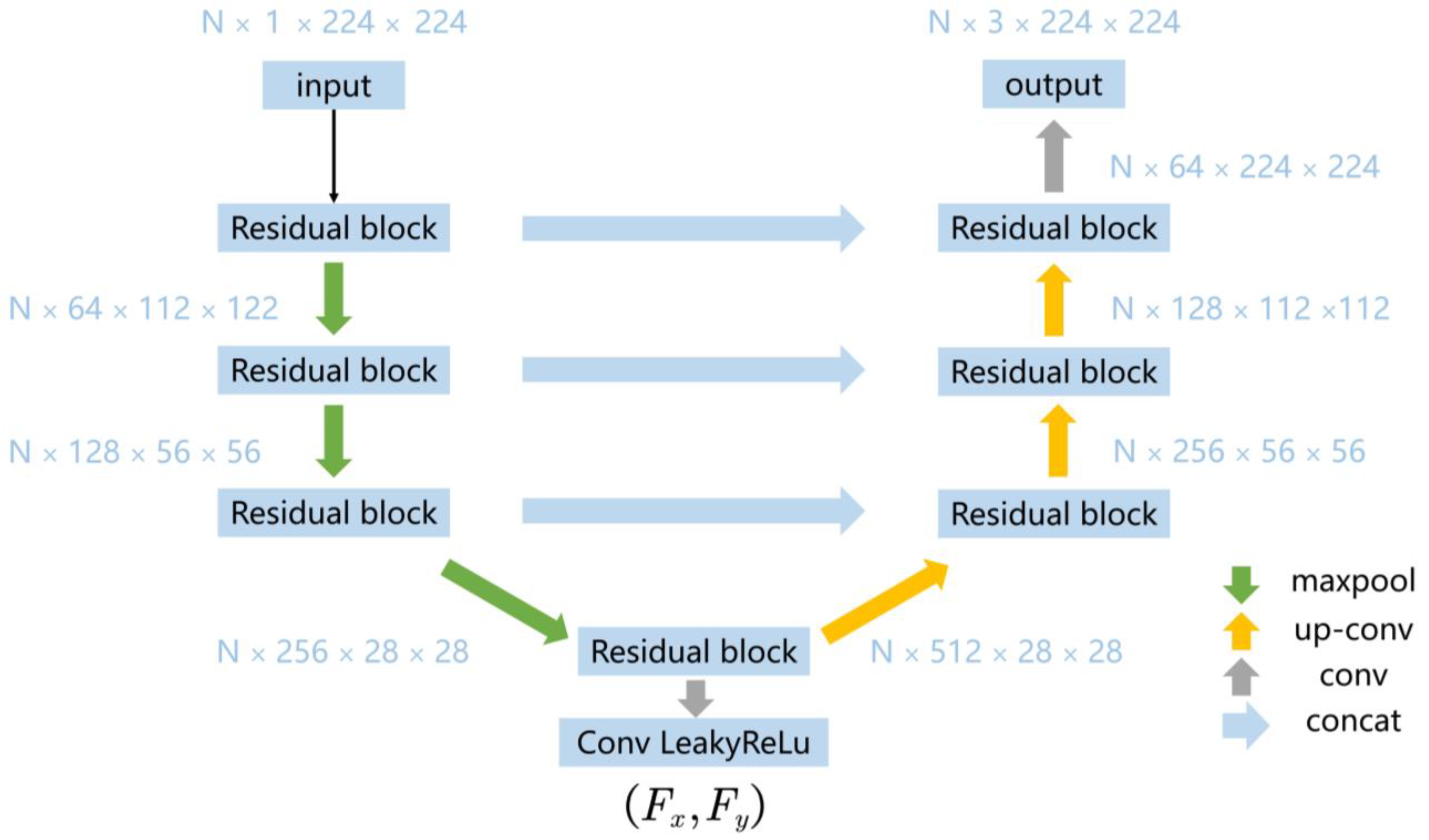
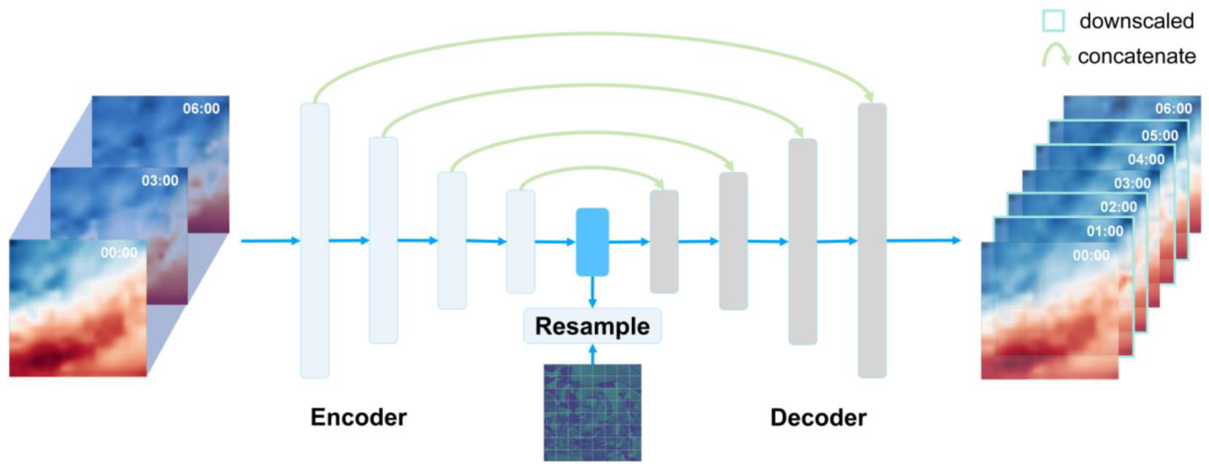
The primary objective of this paper is to introduce a method for temporal downscaling of gridded geophysical data, combining flow regularization techniques with a Residual U-Net architecture, as depicted in Figure 1. The contributions of this paper are threefold:
- We introduce an enhanced residual U-Net architecture for the downscaling of geophysical data. Unlike traditional U-Net architectures, this enhanced model incorporates advection loss in addition to regression loss for training the entire network, so that the model is not overly reliant on fitting to the data (as in pure regression loss) but also considers the underlying physical processes that drive changes in the atmosphere, which allow for a deeper network that can capture complex patterns without succumbing to issues like overfitting or vanishing gradient problems. The depth and architecture of the enhanced residual U-Net are also effective at capturing multi-scale temporal features, a quality lacking in many existing temporal downscaling methods.
- We introduce the concept of flow regularization, which has been traditionally leveraged in computer vision tasks, to the domain of geophysical data downscaling. This addition serves as an auxiliary constraint that guides the model to adhere to the physical laws governing the movement and interaction of geophysical fields with higher accuracy than existing techniques.
- We validate our model using multiple real-world geophysical data sets, comparing its performance against existing methods in terms of accuracy, computational efficiency, and fidelity of temporal features.

Figure 1.
Overview of the residual U-Net model for temporal downscaling. The model consists of an encoder and a decoder, each with four residual blocks. It takes in grid data and outputs data with higher temporal resolution by performing temporal downscaling. After the encoder, the intermediate features are resampled to generate auxiliary flow information, which is then used to calculate the advection loss.
The paper is structured as follows: Section 2 provides a comprehensive review of related work, focusing on the principles of U-Net architectures and residual connections. Section 3 introduces the data sets used for the experiments. Section 4 provides a description of our proposed model, which employs enhanced residual U-Net for temporal downscaling. Section 5 presents the results, offering a comparative analysis with existing methodologies. Section 6 discusses the influence of the input grid data pixel size. Finally, Section 7 concludes the paper by summarizing key findings and outlining avenues for future research.
2. Related Work
2.1. Temporal Downscaling
Temporal downscaling serves as a crucial technique in various scientific applications [29,30,31,32], particularly in environmental modeling where high-frequency fluctuations often matter. The traditional ways to tackle this issue have primarily been statistical. Linear interpolation methods were among the earliest approaches, providing a quick yet overly simplistic way to fill in data between given time points. Soon after, Fourier-based methods were explored to address some of the linear assumptions but found limited applicability due to the inherent cyclical assumptions in the Fourier series [33]. Autoregressive Integrated Moving Average (ARIMA) models gained traction for their capabilities in capturing some level of non-linearity and seasonality [22]. Machine learning techniques like Support Vector Machines (SVMs) and Random Forests have been applied to the temporal downscaling problem as well [19]. Although these methods capture non-linearity better than linear interpolation, they often require extensive feature engineering and parameter tuning. Additionally, they fall short in integrating multi-scale features and incorporating flow information.
2.2. Regularization
In geoscience, regularization techniques are often employed as a critical enforcement mechanism to ensure that model predictions align with physical realities [34]. Some studies have utilized methods such as Total Variation Regularization to maintain crisp boundaries and smooth transitions in geological formations [35]. Others have opted for more intricate, physics-based regularization frameworks like the Hamilton–Jacobi–Bellman equations to enforce dynamic consistency in fluid flow models [36]. Hydrological models frequently make use of an energy balance constraint as a regularization term to confirm the thermodynamic plausibility of predicted water cycles [37]. More recently, advanced methods have emerged that integrate machine learning with physical laws to create hybrid models [38]. These ‘physics-informed’ models use regularization terms sourced from governing equations, like the Navier–Stokes equations for fluid dynamics or the Laplace equation for potential fields, as constraints during the learning process [38,39]. Nonetheless, many of these approaches often come with a trade-off between adherence to physical laws and computational efficiency [40,41]. Our flow regularization technique with advection loss strikes a balance by ensuring compliance with the physical laws that govern geophysical fields, while also being computationally practical.
2.3. Residual Connections
In recent years, residual connections have emerged as a critical innovation in the realm of deep learning architectures, particularly in convolutional neural networks (CNNs). The seminal work by He, et al. [42] introduced residual connections in their ResNet model, demonstrating that these connections alleviate the vanishing gradient problem, thus enabling the training of much deeper networks. Residual architectures have been adopted in various disciplines beyond image classification, including object detection and segmentation. In geoscience applications, residual connections have shown promising results in tasks such as seismic interpretation and subsurface reservoir modeling [43]. These architectures facilitate the learning of hierarchical features from geological data by promoting the flow of gradients throughout the network. By creating shortcuts between layers, residual connections allow for a more efficient and effective propagation of errors during backpropagation, improving the network’s capacity to learn complex mappings.
2.4. U-Net
The U-Net architecture, originally designed for biomedical image segmentation, has shown unparalleled success in various domains requiring complex spatial hierarchies. The architecture follows an encoder-decoder structure, capturing context in the encoding layers and using the decoding layers to reconstruct spatial details. One of the most distinguishing features of the U-Net is its use of skip connections, allowing it to preserve high-frequency details that would otherwise be lost during the encoding process.
In recent years, the U-Net architecture has seen several adaptations and modifications to suit different tasks [44,45,46,47]. For example, 3D U-Nets have been developed to process volumetric data, and Temporal U-Nets have been explored to capture time-related changes in videos [48]. However, integrating temporal downscaling with U-Net’s predominantly spatial-focused architecture remains an open challenge. Few works have attempted to adapt U-Net architectures for time series data, but these generally involve straightforward adaptations that do not fully utilize temporal dependencies. Similarly, while ResNet have been used in conjunction with LSTMs for sequence modeling, their application in temporal downscaling is yet to be fully realized.
In this light, our work aims to fill this gap by proposing a hybrid architecture that leverages the spatial prowess of U-Net, the learning capabilities of ResNet, and the flow regularization techniques, specifically tailored for the task of temporal downscaling in gridded geophysical data.
3. Study Area and Dataset
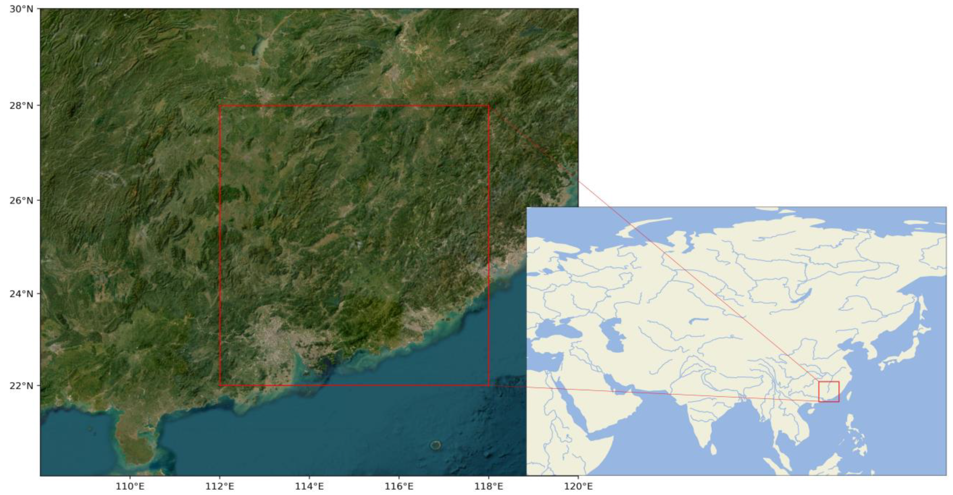
Our investigation targets the geographic region defined by longitudes 112°E to 118°E and latitudes 22°N to 28°N, with a grid resolution of 0.25° × 0.25°, as depicted in Figure 2. The selected region for our downscaling experiments was primarily influenced by its diverse climatic conditions and geographical significance. This area includes a variety of climatic zones, with distinct features ranging from coastal regions to varying inland topographies. This diversity presents an ideal scenario to test the effectiveness of our downscaling model in different climatic settings. Data for this area were sourced from the ERA5 reanalysis dataset. The training dataset is comprised of 21,912 sets, each containing samples from three consecutive hours, spanning the years 2010 to 2019, for a total of 87,648 h. For validation, we use a test set consisting of 2196 sets from the year 2020, also collected at three-hour intervals, totaling 8784 h. Our model aims to downscale these data to a finer one-hour temporal resolution. We evaluate the model’s performance across three meteorological variables: 2 m surface air temperature, 850 hPa geopotential height, and 850 hPa relative humidity. These variables are experimented with separately.
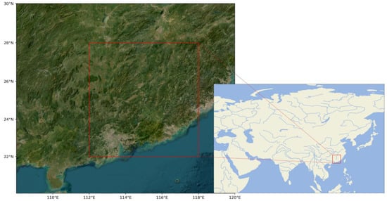
Figure 2.
Study area. The red square indicates the study area.
4. Model
In this section, we describe the architecture and components of our enhanced residual U-Net model. We detail how the model integrates residual blocks, auxiliary flow information, and advection loss to perform temporal downscaling of geophysical data.
4.1. Problem Definition
In the field of geophysical data analysis, the problem of temporal downscaling aims to refine the time resolution of observed data, thereby providing more frequent measurements. Specifically, given a dataset at a coarser temporal resolution of three hours, the objective is to estimate a fine-grained dataset at a one-hour resolution, where for . Here, represents the number of samples, denotes the horizontal dimensions, and denotes the vertical dimensions. The primary goal is to minimize the discrepancy between the ground truth and the predicted over the fine-grained temporal intervals. Mathematically, this can be formulated as
Here, represents the parameters of the Enhanced Residual U-Net model, and is the loss function.
4.2. Residual U-Net
In this work, we introduce an architecture, enhanced residual U-Net, designed for the temporal downscaling of gridded geophysical data. This architecture merges the high-level feature extraction capabilities of U-Net with the robustness of Residual Networks (ResNet) to produce an efficient and scalable model (see Figure 3).

Figure 3.
The architecture of the residual U-Net. It consists of an encoder section on the left, a decoder section on the right, and an auxiliary flow information layer in between. The encoder features four residual blocks, each containing two convolutional layers with batch normalization and ReLU activation functions, responsible for reducing feature dimensions while capturing initial patterns from the input. The decoder also contains four residual blocks and uses transposed convolutions for upsampling. Skip connections merge the output from each encoder Residual Block with its corresponding decoder block, ensuring the preservation of spatial information across scales.
The architecture is constructed from two main components: an encoder and a decoder. The encoder is responsible for downscaling the input tensor, thereby extracting high-level features. The decoder, on the other hand, upscales these high-level features to reconstruct the output tensor. These operations are standard in any U-Net architecture; however, our model introduces several enhancements.
One of the enhancements in our architecture is the introduction of residual blocks following key convolutional layers in the encoder section. The architecture’s depth is primarily achieved through its deeper residual blocks, and each residual block comprises three 3 3 convolutional layers with ReLU activations [49]. The outputs of these layers are summed with the original input using a skip connection and these residual blocks help the model to learn complex features with reduced risk of vanishing or exploding gradients.
The encoder section is composed of a succession of four deeper residual blocks, each with distinct channel configurations—64, 128, 256, and 512 channels. Every deeper residual block comprises three convolutional layers, each followed by batch normalization and ReLU activation functions. This series of operations enriches the representation of the input data by sequentially increasing the number of channels. The architecture also incorporates max-pooling layers after each block to reduce the spatial dimensions of the feature maps. Subsequent to each max-pooling operation, the spatial dimensions are halved, thereby focusing on the extraction of high-level features.
The decoder section reverses the operations conducted by the encoder. It employs a series of up-convolutional layers paired with concatenation operations that merge high-level features from the encoder. Each up-convolutional layer also employs a ReLU activation function and effectively doubles the spatial dimensions. Similar to the encoder, residual blocks are also introduced in the decoder. These are positioned after each up-convolutional layer and function in the same manner as their encoder counterparts. These blocks refine the combined high-level and low-level features. The network concludes with a 1 1 convolutional layer, which condenses the 64-channel feature map into a two-channel output.
4.3. Flow Regularization Using Advection Loss
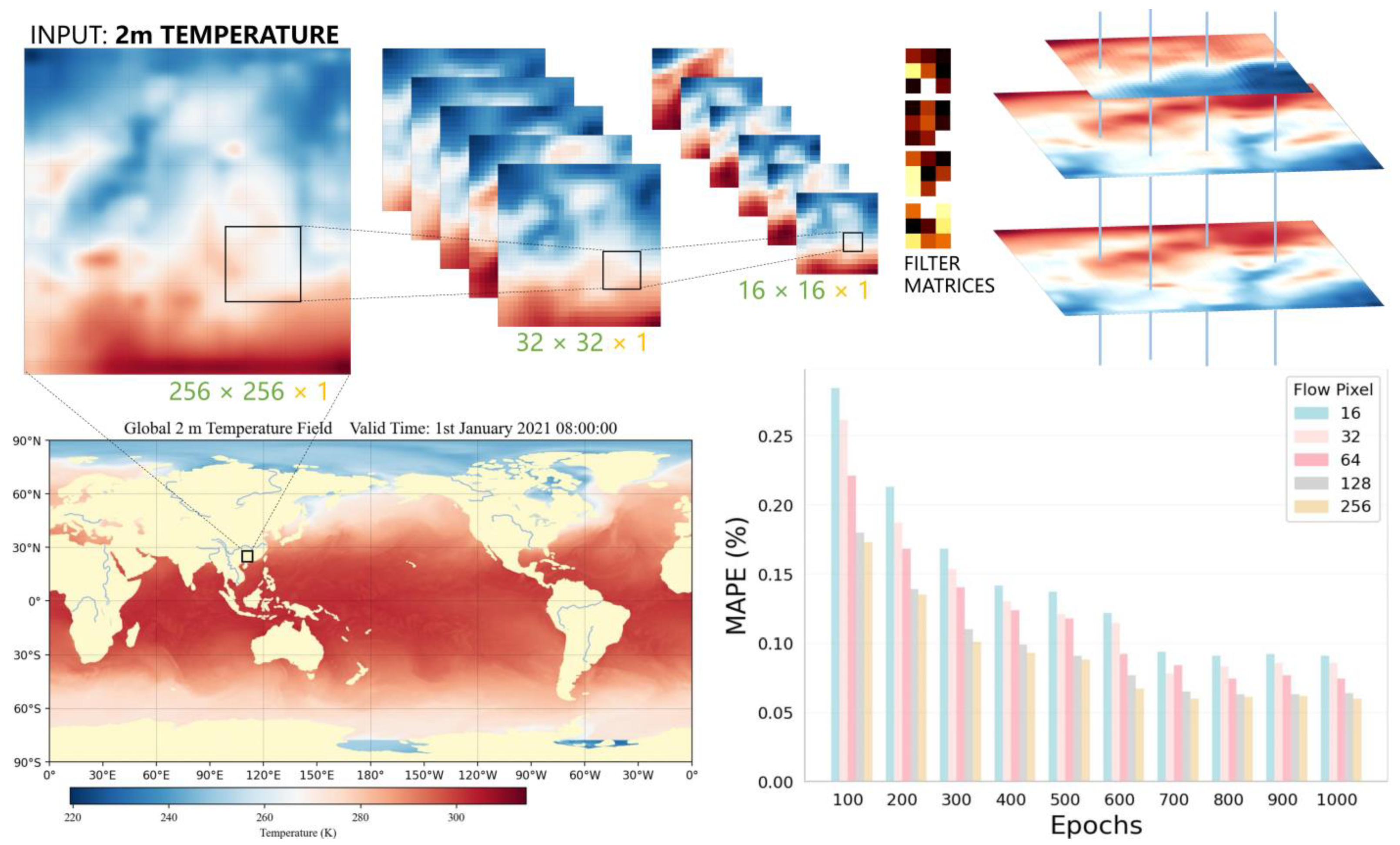
Conventional methods often miss capturing the evolving patterns. To address this limitation, we incorporate flow information with advection loss into our enhanced residual U-Net model, and this section details the mathematical and computational elements of this approach (see Figure 4).

Figure 4.
Overview of flow information extraction from the intermediate features post-encoder phase. Following encoding, these intermediate features undergo specific convolutional operations and resampling procedures to yield the flow information. The bar chart illustrates the Mean Absolute Percentage Error (MAPE) for various flow pixel resolutions across different epochs. The x-axis represents the training epochs, ranging from 100 to 1000, while the y-axis represents the MAPE in percentages.
Advection refers to the transport of a scalar field driven by flow regularization. Mathematically, it can be represented as a transformation function, , which takes in a geophysical field at time , denoted as , and flow information , and returns an approximated field at time , represented as . The principle behind advection is rooted in fluid dynamics and is used widely in computational fluid dynamics simulations and meteorological models. By adopting an advection transformation, we impose an auxiliary constraint on our neural network model, compelling it to learn physically meaningful dynamics.
The advection loss is introduced as an additional term in the loss function and is defined as . In essence, this loss measures the difference between the true field at and the advected field . It guides the network to learn a more accurate representation of the data and acts as a regularization term, reducing overfitting while still ensuring that the model learns the dynamics of the field.
For the computation of , spatial interpolation is employed. Given a 2D geophysical field and corresponding flow information, which is also a 2D tensor but with two channels representing the velocity vectors , each point in is shifted according to the velocity vector at that point. Specifically, and are the latitudinal and longitudinal components of the velocity at each point in a given field. This means that for each point, indicates the rate and direction of movement along the horizontal axis, while represents the same along the vertical axis. The new coordinates are calculated as . Bilinear interpolation is used to estimate the value of the advected field at these new coordinates.
The final loss function incorporating both the L2 loss and the advection loss is formulated as follows:
In this equation, is the L2 loss, representing the squared Euclidean distance between the predicted output and the ground-truth . The term is the weighted advection loss, and the weight of is applied to balance the contribution of advection loss against the L2 loss. refers to the next immediate true data sample, which is either an hour or two hours apart.
5. Experiments
The model was implemented using PyTorch and the training was performed on a machine equipped with eight NVIDIA Tesla A5000 GPUs. During training, we employed the Adam optimizer with a learning rate of 0.0001 and a batch size of 32. The model was trained for 1000 epochs. A decay rate of 0.9 for the learning rate was applied every 200 epochs to ensure convergence. The loss function used in training was a combination of the Mean Squared Error (MSE) loss and the advection loss, as described in Section 4.3.
5.1. Quantitative Comparison with Conventional Methods
In this section, we conduct a quantitative evaluation of our enhanced residual U-Net model against several benchmark methods, focusing on three critical atmospheric variables: 2 m air temperature, geopotential height, and relative humidity. For a robust comparison, we employ three well-established metrics: Root Mean Square Error (RMSE), Mean Absolute Error (MAE), and Mean Absolute Percentage Error (MAPE). Linear interpolation was directly applied by averaging adjacent temporal data points, assuming uniform change over time. Cubic spline interpolation employed a piecewise third-order polynomial, enhancing smoothness and fitting the data’s curvature better than the linear method. We also trained three computer vision models specifically for weather data, training from scratch rather than using pre-trained weights. These models, typically used for video frame interpolation, were employed to handle meteorological inputs by converting meteorological fields from single-channel data to three-channel format, without modifying the main backbone. The models’ input and output layers were the only components modified to process our weather dataset.
As depicted in Table 1, it is clear that our enhanced residual U-Net model surpasses other techniques across all three metrics and for each atmospheric variable examined. Specifically, for 2 m air temperature, our model yields RMSE and MAE values of 0.20 and 0.17, respectively; for geopotential height, the corresponding values are 0.72 and 0.62; and for relative humidity, these metrics stand at 0.64, 0.46, and 0.59%.

Table 1.
Comparison of different methods for temporal downscaling.
When contrasted with conventional methods like linear interpolation and cubic spline—whose performance metrics are considerably higher in terms of RMSE and MAE—the superiority of our model becomes evident. The results are presented in Table 1. Although these deep learning-based models outperform linear interpolation and cubic spline, they still fail to match the superior performance of our enhanced residual U-Net model.
5.2. Visual and Qualitative Analysis
To assess the effectiveness of our model, we selected a case of the 2 m temperature fields for 21 January 2020, between the hours of 10:00 and 17:00. As depicted by Figure 5, our model accurately reproduces the nonlinear variability in the temperature field.

Figure 5.
Ground truth and model-generated downscaled results. Points at 10 a.m., 1 p.m., 2 p.m., and 5 p.m. are the model’s input, while the data at 11 a.m., 12 p.m., 3 p.m., and 4 p.m. are model-generated outputs. The black square indicates the study area.
Focusing on specific intervals, for the 11:00 downscaling between 10:00 and 13:00, the temperature patterns exhibit distinct characteristics. For example, the coastal areas, which originally showed a relatively warmer temperature at 10:00, start showing moderate cooling due to oceanic influences. In contrast, the central regions, which were cooler at 10:00, warm up slightly, likely due to increased solar radiation. This is captured with an RMSE of 0.22, MAE of 0.19, and MAPE of 0.06%. As we move to 12:00, the temperature in the valley regions starts showing minor fluctuations, likely due to local wind patterns. The RMSE improves to 0.20, MAE drops to 0.17, and the MAPE remains stable at 0.06%, emphasizing the model’s competence in capturing these subtle dynamics.
Between 14:00 and 17:00, the 15:00 downscaling indicates that urban areas start to experience heat island effects, with temperature spikes in densely populated zones. These spikes contrast with adjacent rural or forested areas that show a more stable temperature profile. At this point, the RMSE is 0.20, MAE is 0.18, and the MAPE is stable at 0.06%. At 16:00, there is a notable decrease in temperature in the mountainous regions, likely due to the shadows cast by the changing sun angle. This dynamic is reflected with an RMSE of 0.19, MAE of 0.16, and a consistent MAPE of 0.06%.
5.3. Ablation Studies
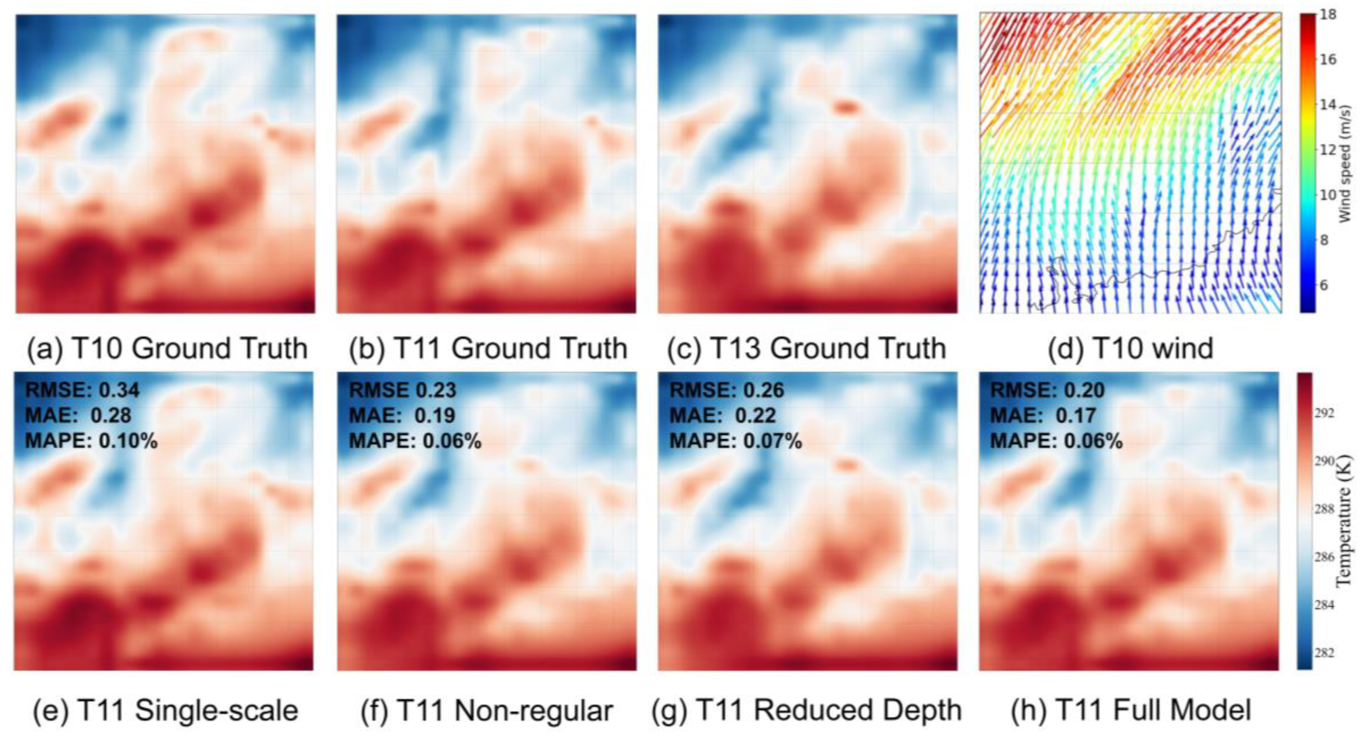
In our ablation studies, we examine the individual components of the enhanced residual U-Net model to understand their significance in achieving overall performance metrics (see Figure 6). We set the performance of the full model as the baseline, which exhibits RMSE and MAE values of 0.20 and 0.17 for 2 m temperature, 0.72 and 0.62 for geopotential height, and 0.64 and 0.46 for relative humidity. To remove multi-scale features in the U-Net for our ablation study, we simply omit the skip connections. This is accomplished by not using the ‘torch.cat’ operation to merge features from the encoder and decoder, thus preventing the combination of high-resolution details with low-resolution context. Upon removing the multi-scale features, we observed a discernible decrease in predictive accuracy across all variables, with RMSE and MAE values for 2 m temperature rising to 0.34 and 0.28, respectively (see Table 2). This confirms the importance of multi-scale features in capturing the complexity of geophysical data. When we omitted the flow regularization, there was a significant performance decline: RMSE and MAE values for 2 m temperature rose to 0.23 and 0.19, indicating the benefits of incorporating flow regularization to capture temporal dynamics effectively. Lastly, reducing the architectural depth of the model led to a less pronounced, yet still noticeable, decline in performance. For instance, RMSE for the 2 m temperature increased to 0.26, and MAE rose to 0.22, underlining the model’s depth’s role in capturing the intricacies of geophysical data. Overall, the degradation in model performance upon the removal of each component underscores their collective importance, reinforcing the need for their inclusion in the final architecture.
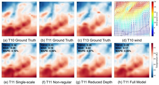
Figure 6.
Visual comparison of ablation study results. We downscale the 2 m temperature fields from 10 a.m. to 1 p.m. on 21 January 2020, to obtain results for 11 a.m. Subfigure d depicts the wind field at 11 a.m., which offers indicative insights into temperature evolution.

Table 2.
Ablation study on the effect of various components on the model’s performance.
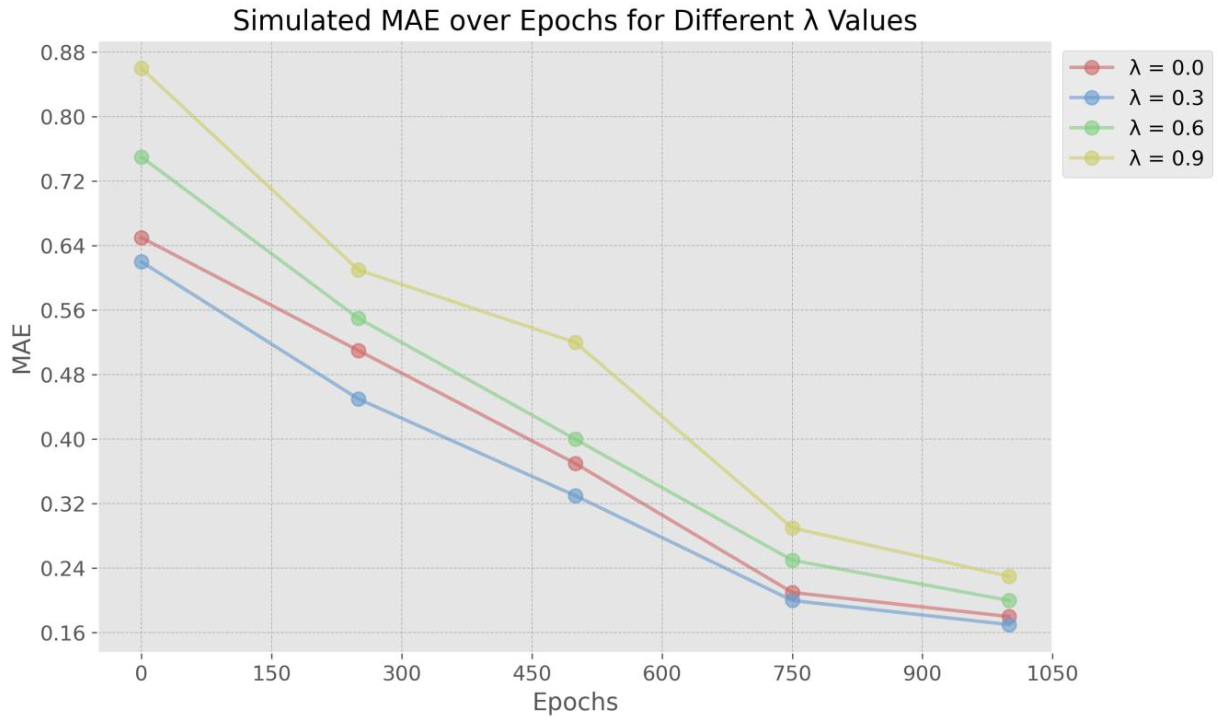
In our ablation study concerning the advection loss weight , we explore the statistical significance of its calibration for the accuracy of temporal downscaling in geophysical data. The detailed line chart in our manuscript illustrates how the mean absolute error (MAE) varies with different settings. With set to 0.3, the model achieves the lowest MAE values, suggesting that this level maximizes the benefit of incorporating flow information while also allowing for local atmospheric dynamics, such as radiative heating or cooling, to be adequately represented. On the other hand, a high value, such as 0.9, results in increased MAE, indicating a diminished ability to capture these local changes, as the model overly emphasizes adherence to the advected state. Conversely, the absence of advection loss () leads to increased errors, highlighting the necessity of this term for improving downscaling accuracy.
6. Discussion
In our analysis, we found that the input grid data pixel size significantly influences the model’s Mean Absolute Error (MAE), forming a U-shaped pattern, as depicted in Figure 7. For smaller pixel sizes, specifically at 64 pixels, the MAE was around 0.26. The convolutional layers in this case are restricted to localized features, missing the larger spatial context that is crucial for accurate downscaling. Conversely, the MAE reaches its minimum value of 0.17 at an optimal pixel size of 224 (see Figure 8). Beyond this optimal point, the MAE starts to increase again, climbing to approximately 0.33 at a pixel size of 320. This suggests that while the model is effective in capturing global features at larger pixel sizes, it fails to grasp finer details, leading to increased error.
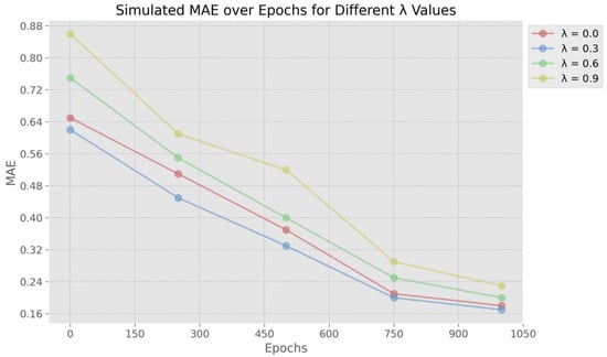
Figure 7.
Model performance with different values.
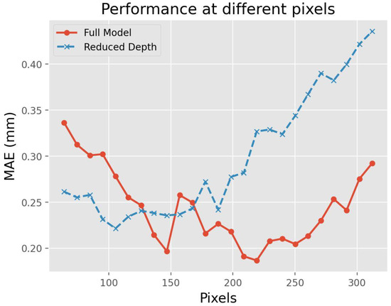
Figure 8.
Influence of field pixels. In the experiments, the size of the selected area remains unchanged, but the dimensions of the input data are altered through bicubic interpolation.
This performance is further illuminated when comparing the MAE curves between the full model and the reduced-depth model. The full model achieved a lower minimum MAE value of 0.17 as opposed to the reduced model’s 0.22. This can largely be attributed to the residual modules in the full model, which allow for a more efficient and resilient feature extraction process. These modules facilitate better generalization across varying pixel sizes, thus accounting for the full model’s more effective U-shaped performance curve in MAE across a broader range of pixel sizes.
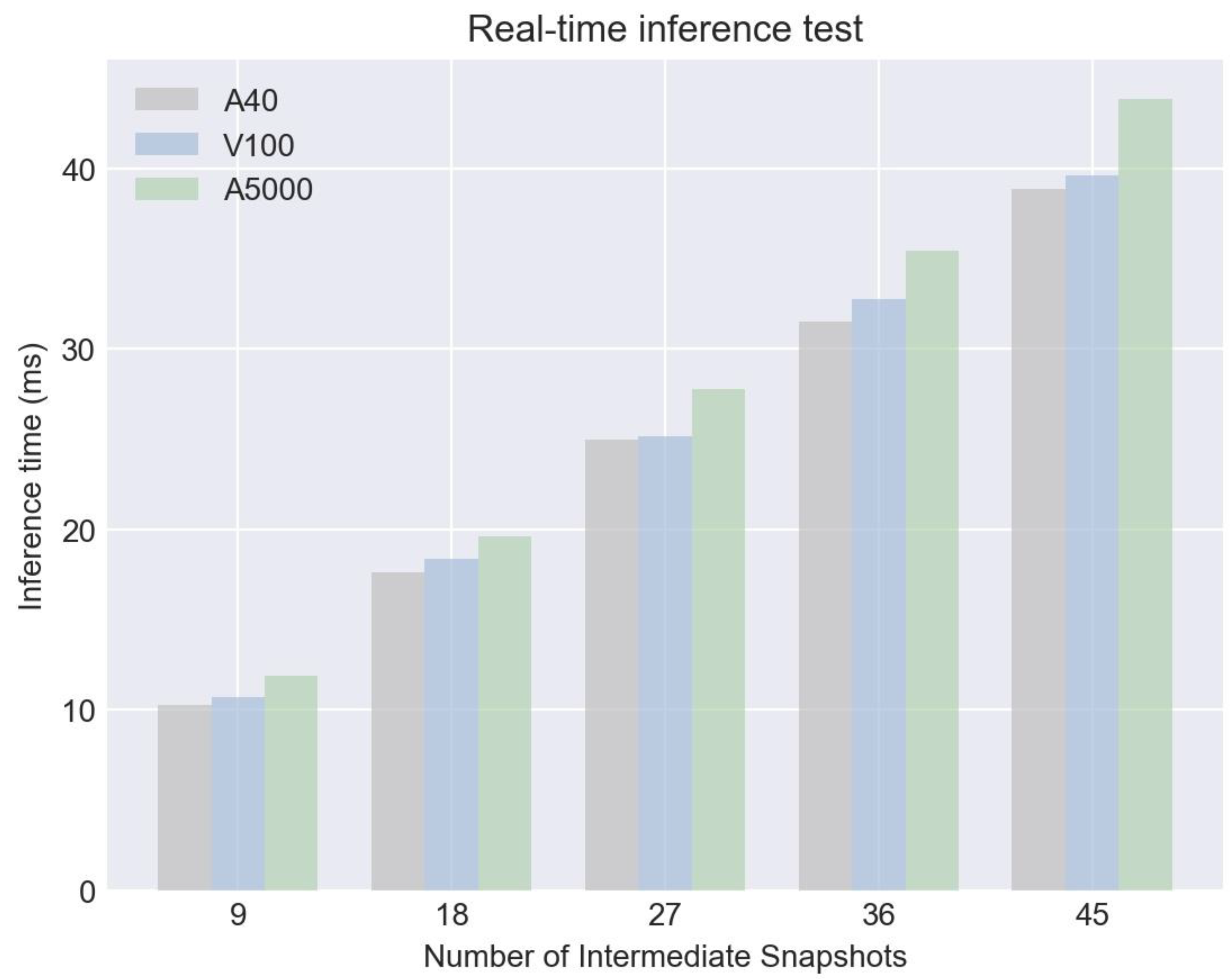
In addition to the performance metrics discussed earlier, another significant advantage of our model is its capability to support real-time inference (see Figure 9). A set of experiments was conducted to evaluate the model’s speed performance across multiple hardware configurations—A40, V100, and A5000. The inference time was observed at different intermediate snapshot levels: 9, 18, 27, 36, and 45. Remarkably, even at 45 intermediate snapshots, the inference time did not exceed 44 ms on A5000, and it was even lower on A40 and V100 setups, clocking at approximately 39 ms and 38 ms, respectively. This rapid inference time positions our model as not only accurate but also highly practical for real-time applications in weather forecasting and climate studies.
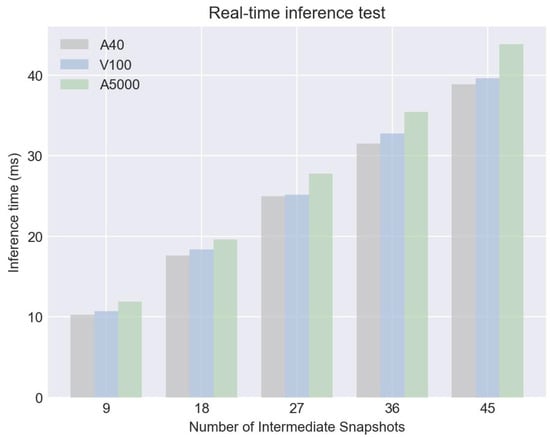
Figure 9.
Comparison of inference time under different GPU conditions.
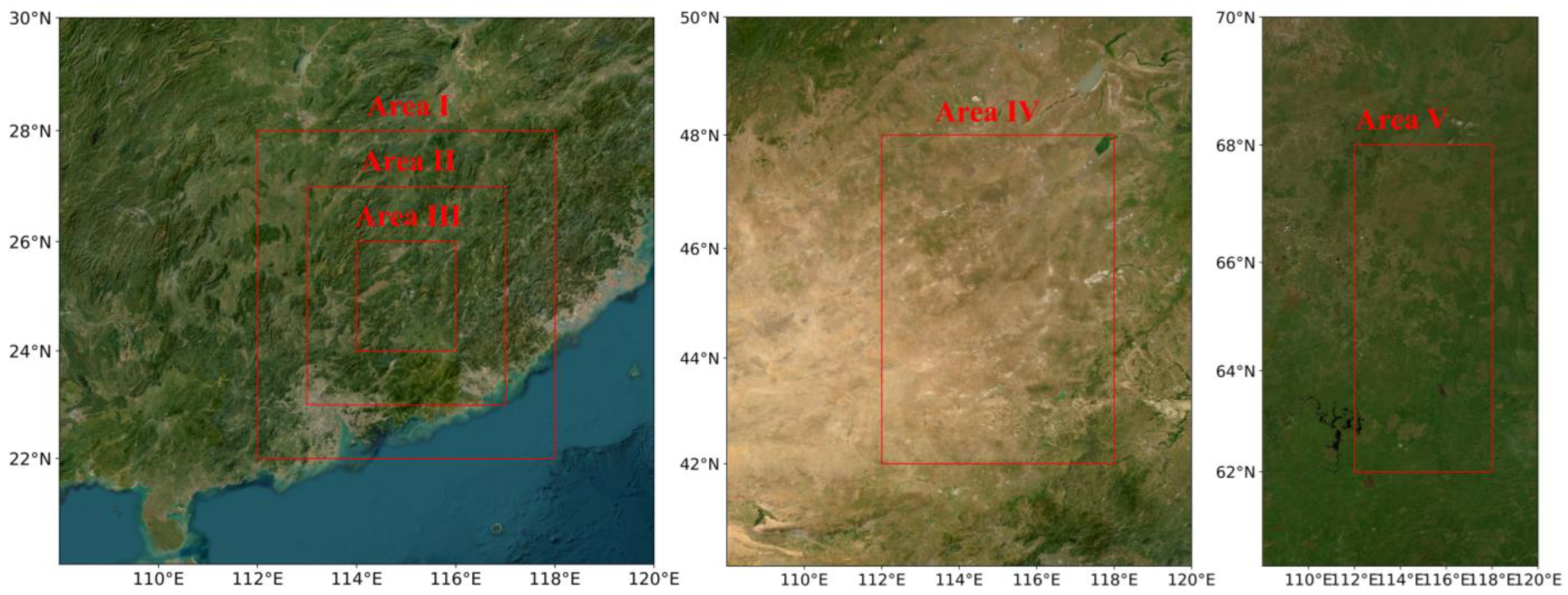
To assess the impact of spatial domain size on temporal downscaling accuracy, our study conducted tests across three increasingly localized areas within the ERA5 dataset’s 0.25° resolution grid (see Figure 10). Area I spans longitudes 112°E to 118°E, Area II narrows down to 113°E to 117°E, and Area III further reduces to 114°E to 116°E. The intent was to understand how the extent of spatial information affects the prediction quality for a specific grid cell’s temporal downscaling. The results, as shown in Table 3, indicate a nuanced relationship between spatial domain size and downscaling accuracy. In Areas I, II, and III, we observed RMSE, MAE, and MAPE values of 0.20/0.17/0.06%, 0.17/0.18/0.06%, and 0.17/0.14/0.05%, respectively. This pattern suggests that as the spatial domain becomes more localized, the model’s performance slightly improves in terms of RMSE and MAPE, while the MAE shows a minor increase from Area II to Area III. Our findings suggest that reducing the spatial domain helps the model to focus on more relevant atmospheric features specific to the area, enhancing the precision of temporal downscaling. This is particularly evident in Area III, where the smallest spatial extent was associated with the lowest RMSE and MAPE, indicating a refined prediction capability. However, the slight increase in MAE from Area II to III highlights the complexity of balancing spatial resolution with predictive accuracy. The increasing error rates in temporal downscaling from Areas I (22°N–28°N) to Area V (62°N–68°N) can be attributed to the complex atmospheric dynamics and pronounced seasonal variations typical of higher latitudes. Area I shows the lowest error rates (RMSE: 0.20, MAE: 0.17), indicating better model performance in lower latitudes. In contrast, Areas IV and V exhibit progressively higher errors, with Area V reaching an RMSE of 0.26 and an MAE of 0.20. These higher latitudes face challenges like greater temperature shifts between seasons, more complex weather systems like jet streams, and data sparsity due to fewer weather stations. These factors combined make accurate temporal downscaling more challenging in higher latitude regions.
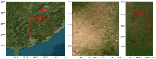
Figure 10.
Illustration of five selected areas, labeled Area I to Area V, showcasing the variations in both spatial extent and latitude. Area I, Area II, and Area III represent regions where the spatial domain progressively decreases in size, providing a comparative perspective on how varying spatial scales influence the model’s performance. Additionally, Area I, Area IV, and Area V are arranged in ascending order of latitude, allowing for an examination of the impact of latitudinal differences on the effectiveness of temporal downscaling.

Table 3.
Generalization test at different spatial resolutions on 2 m temperature fields.
This study primarily uses a 5 × 5 convolutional kernel size for temporal downscaling. The comparison between different kernel sizes—3 × 3, 5 × 5, and 7 × 7—reveals differences in their performance, as shown in Table 4. The 5 × 5 kernel size showed the most consistent and favorable results across the Full Model and the Reduced Depth model in terms of RMSE, MAE, and MAPE metrics. The 3 × 3 kernel displayed slightly higher errors than the 5 × 5 kernel, indicating slightly diminished performance in capturing temporal dependencies. Meanwhile, the 7 × 7 kernel size resulted in higher error metrics for both models, indicating reduced accuracy in temporal downscaling. The overall trend suggests that the 5 × 5 kernel size excels in extracting relevant features and capturing temporal patterns more effectively within the context of the temporal downscaling task carried out in this research.

Table 4.
Performance of models with different convolutional kernel sizes.
7. Conclusions
In this study, we introduced the enhanced residual U-Net, which incorporates advection loss in addition to regression loss for training and combines the strengths of U-Net and ResNet to address the challenge of temporal downscaling in gridded geophysical data. The architecture is specifically designed to harness both local and global features within the data, thereby producing a robust and versatile model capable of delivering high-quality downscaling results. The residual U-Net has been applied in many other fields [51,52,53,54] (including spatial downscaling), and we are the first to apply it in the domain of temporal downscaling. This design choice not only enhances the learning capability of the network but also alleviates issues related to the vanishing gradient problem, allowing for deeper and more effective networks. We also introduced a custom loss function that combines Mean Squared Error (MSE) with a spatial regularization term, which collectively ensures both the fidelity and spatial coherence of the downscaled output.
Our experimental results, based on a comprehensive evaluation using multiple gridded geophysical datasets, validated the effectiveness of the enhanced residual U-Net model. We demonstrated that the architecture outperformed traditional downscaling methods and other state-of-the-art machine learning approaches in key metrics, including RMSE and MAE, while maintaining computational efficiency.
In conclusion, the enhanced residual U-Net architecture stands as a robust and efficient solution for the temporal downscaling of gridded geophysical data. Its design features, including the use of residual blocks and a custom loss function, make it a highly promising tool for both academic research and practical applications in the field of geoscience.
Future work could further enhance this architecture by incorporating additional techniques for feature selection or by tailoring the network to different kinds of geophysical data. Moreover, real-world applicability of this model could be tested in other domains requiring high-fidelity downscaling, providing a broader utility beyond the specific use-case studied here.
Author Contributions
Conceptualization, L.W. and Q.L. (Qian Li); methodology, L.W.; software, L.W.; validation, Q.L. (Qian Li) and Q.L. (Qi Lv); formal analysis, L.W.; investigation, Q.L. (Qian Li); resources, X.P.; data curation, L.W.; writing—original draft preparation, L.W.; writing—review and editing, Q.L. (Qi Lv); visualization, Q.L. (Qi Lv); supervision, Q.L. (Qian Li); project administration, Q.L. (Qian Li); funding acquisition, Q.L. (Qian Li). All authors have read and agreed to the published version of the manuscript.
Funding
This research was funded by the National Natural Science Foundation of China (Grant No. U2242201, 42075139, 42105146, 41305138), the China Postdoctoral Science Foundation (Grant No. 2017M621700), Hunan Province Natural Science Foundation (Grant No. 2021JC0009, 2021JJ30773, 2023JJ30627), and Fengyun Application Pioneering Project (FY-APP-2022.0605).
Data Availability Statement
All data necessary to reproduce the results of this work can be downloaded at the ERA5 Climate Data Store via https://doi.org/10.24381/cds.bd0915c6 and https://doi.org/10.24381/cds.adbb2d47, accessed on 12 April 2023.
Conflicts of Interest
The authors declare no conflicts of interest.
References
- Reichstein, M.; Camps-Valls, G.; Stevens, B.; Jung, M.; Denzler, J.; Carvalhais, N.; Prabhat, F. Deep learning and process understanding for data-driven Earth system science. Nature 2019, 566, 195–204. [Google Scholar] [CrossRef] [PubMed]
- Scipal, K.; Holmes, T.R.H.; de Jeu, R.A.M.; Naeimi, V.; Wagner, W. A possible solution for the problem of estimating the error structure of global soil moisture data sets. Geophys. Res. Lett. 2008, 35, 24. [Google Scholar] [CrossRef]
- Chen, S.; Zhang, M.; Lei, F. Mapping Vegetation Types by Different Fully Convolutional Neural Network Structures with Inadequate Training Labels in Complex Landscape Urban Areas. Forests 2023, 14, 1788. [Google Scholar] [CrossRef]
- Marthews, T.R.; Dadson, S.J.; Lehner, B.; Abele, S.; Gedney, N. High-resolution global topographic index values for use in large-scale hydrological modelling. Hydrol. Earth Syst. Sci. 2015, 19, 91–104. [Google Scholar] [CrossRef]
- Loew, A.; Bell, W.; Brocca, L.L.; Bulgin, C.E.; Burdanowitz, J.; Calbet, X.; Donner, R.V.; Ghent, D.; Gruber, A.; Kaminski, T.; et al. Validation practices for satellite-based Earth observation data across communities. Rev. Geophys. 2017, 55, 779–817. [Google Scholar] [CrossRef]
- Mann, M.E.; Rahmstorf, S.; Kornhuber, K.; Steinman, B.A.; Miller, S.K.; Coumou, D. Influence of Anthropogenic Climate Change on Planetary Wave Resonance and Extreme Weather Events. Sci. Rep. 2017, 7, 1–12. [Google Scholar] [CrossRef]
- Rogelj, J.; Forster, P.M.; Kriegler, E.; Smith, C.J.; Séférian, R. Estimating and tracking the remaining carbon budget for stringent climate targets. Nature 2019, 571, 335–342. [Google Scholar] [CrossRef]
- Mason, S.J.; Stephenson, D.B. How Do We Know Whether Seasonal Climate Forecasts are Any Good. In Seasonal Climate: Forecasting and Managing Risk; Springer: Dordrecht, The Netherlands, 2008; pp. 259–289. [Google Scholar]
- Schloss, A.; Kicklighter, D.W.; Kaduk, J.; Wittenberg, U.; ThE Participants OF ThE Potsdam NpP Model Intercomparison. Comparing global models of terrestrial net primary productivity (NPP): Comparison of NPP to climate and the Normalized Difference Vegetation Index (NDVI). Glob. Chang. Biol. 1999, 5, 25–34. [Google Scholar] [CrossRef]
- Schleussner, C.; Lissner, T.; Fischer, E.M.; Wohland, J.; Perrette, M.; Golly, A.; Rogelj, J.; Childers, K.H.; Schewe, J.; Frieler, K.; et al. Differential climate impacts for policy-relevant limits to global warming: The case of 1.5 °C and 2 °C. Earth Syst. Dyn. Discuss. 2015, 7, 327–351. [Google Scholar] [CrossRef]
- Fowler, H.J.; Blenkinsop, S.; Tebaldi, C. Linking climate change modelling to impacts studies: Recent advances in downscaling techniques for hydrological modelling. Int. J. Climatol. 2007, 27, 1547–1578. [Google Scholar] [CrossRef]
- Mearns, L.; Giorgi, F.; Whetton, P.H.; Pabón, D.; Hulme, M.; Lal, M. Guidelines for Use of Climate Scenarios Developed from Regional Climate Model Experiments. Data Distrib. Cent. Intergov. Panel Clim. Chang. 2003, 38. [Google Scholar]
- Challinor, A.J.; Watson, J.E.M.; Lobell, D.; Howden, S.M.; Smith, D.R.; Chhetri, N. A meta-analysis of crop yield under climate change and adaptation. Nat. Clim. Chang. 2014, 4, 287–291. [Google Scholar] [CrossRef]
- Gupta, R.; Yadav, A.K.; Jha, S.; Pathak, P.K. Time Series Forecasting of Solar Power Generation Using Facebook Prophet and XG Boost. In Proceedings of the 2022 IEEE Delhi Section Conference (DELCON), New Delhi, India, 11–13 February 2022; pp. 1–5. [Google Scholar]
- Monteith, J.L.; Oke, T.R. Boundary Layer Climates. J. Appl. Ecol. 1979, 17, 517. [Google Scholar] [CrossRef]
- Salehnia, N.; Hosseini, F.S.; Farid, A.; Kolsoumi, S.; Zarrin, A.; Hasheminia, M. Comparing the Performance of Dynamical and Statistical Downscaling on Historical Run Precipitation Data over a Semi-Arid Region. Asia-Pac. J. Atmos. Sci. 2019, 55, 737–749. [Google Scholar] [CrossRef]
- Global Circulation Models. In Proceedings of the ACM SIGSPATIAL International Workshop on Advances in Geographic Information Systems (SIGSPATIAL 2017), Redondo Beach, CA, USA, 7 November 2017.
- Kisembe, J.; Favre, A.; Dosio, A.; Lennard, C.J.; Sabiiti, G.; Nimusiima, A. Evaluation of rainfall simulations over Uganda in CORDEX regional climate models. Theor. Appl. Climatol. 2018, 137, 1117–1134. [Google Scholar] [CrossRef]
- Vandal, T.J.; Kodra, E.; Ganguly, A.R. Intercomparison of machine learning methods for statistical downscaling: The case of daily and extreme precipitation. Theor. Appl. Climatol. 2017, 137, 557–570. [Google Scholar] [CrossRef]
- Tang, J.; Niu, X.; Wang, S.; Gao, H.; Wang, X.; Wu, J. Statistical downscaling and dynamical downscaling of regional climate in China: Present climate evaluations and future climate projections. J. Geophys. Res. Atmos. 2016, 121, 2110–2129. [Google Scholar] [CrossRef]
- Isotta, F.A.; Begert, M.; Frei, C. Long-Term Consistent Monthly Temperature and Precipitation Grid Data Sets for Switzerland Over the Past 150 Years. J. Geophys. Res. Atmos. 2019, 124, 3783–3799. [Google Scholar] [CrossRef]
- ArunKumar, K.E.; Kalaga, D.V.; Mohan Sai Kumar, C.; Kawaji, M.; Brenza, T.M. Comparative analysis of Gated Recurrent Units (GRU), long Short-Term memory (LSTM) cells, autoregressive Integrated moving average (ARIMA), seasonal autoregressive Integrated moving average (SARIMA) for forecasting COVID-19 trends. Alex. Eng. J. 2022, 61, 7585–7603. [Google Scholar] [CrossRef]
- Majda, A.J.; Harlim, J. Physics constrained nonlinear regression models for time series. Nonlinearity 2012, 26, 201–217. [Google Scholar] [CrossRef]
- Yang, H.; Wang, T.; Zhou, X.; Dong, J.; Gao, X.; Niu, S. Quantitative Estimation of Rainfall Rate Intensity Based on Deep Convolutional Neural Network and Radar Reflectivity Factor. In Proceedings of the 2nd International Conference on Big Data Technologies, Jinan, China, 28 August 2019; pp. 244–247. [Google Scholar]
- Misra, S.; Sarkar, S.; Mitra, P. Statistical downscaling of precipitation using long short-term memory recurrent neural networks. Theor. Appl. Climatol. 2018, 134, 1179–1196. [Google Scholar] [CrossRef]
- Xiang, X.; Tian, Y.; Zhang, Y.; Fu, Y.R.; Allebach, J.P.; Xu, C. Zooming Slow-Mo: Fast and Accurate One-Stage Space-Time Video Super-Resolution. In Proceedings of the 2020 IEEE/CVF Conference on Computer Vision and Pattern Recognition (CVPR), Seattle, WA, USA, 13–19 June 2020; pp. 3367–3376. [Google Scholar]
- Jiang, H.; Sun, D.; Jampani, V.; Yang, M.-H.; Learned-Miller, E.G.; Kautz, J. Super SloMo: High Quality Estimation of Multiple Intermediate Frames for Video Interpolation. In Proceedings of the 2018 IEEE/CVF Conference on Computer Vision and Pattern Recognition, Salt Lake City, UT, USA, 18–23 June 2018; pp. 9000–9008. [Google Scholar]
- Lees, T.; Buechel, M.; Anderson, B.; Slater, L.J.; Reece, S.; Coxon, G.; Dadson, S.J. Rainfall-Runoff Simulation and Interpretation in Great Britain using LSTMs. In Proceedings of the 23rd EGU General Assembly, Online, 19–30 April 2021. EGU21-2778. [Google Scholar]
- Kajbaf, A.A.; Bensi, M.T.; Brubaker, K.L. Temporal downscaling of precipitation from climate model projections using machine learning. Stoch. Environ. Res. Risk Assess. 2022, 36, 2173–2194. [Google Scholar] [CrossRef]
- Barboza, L.A.; Chen, S.; Alfaro-Córdoba, M. Spatio-temporal downscaling emulator for regional climate models. Environmetrics 2022, 34, e2815. [Google Scholar] [CrossRef]
- Huang, J.; Perez, M.J.R.; Perez, R.; Yang, D.; Keelin, P.; Hoff, T.E. Nonparametric Temporal Downscaling of GHI Clearsky Indices using Gaussian Copula. In Proceedings of the 2022 IEEE 49th Photovoltaics Specialists Conference (PVSC), Philadelphia, PA, USA, 5–10 June 2022; pp. 0654–0657. [Google Scholar]
- Michel, A.; Sharma, V.; Lehning, M.; Huwald, H. Climate change scenarios at hourly time-step over Switzerland from an enhanced temporal downscaling approach. Int. J. Climatol. 2021, 41, 3503–3522. [Google Scholar] [CrossRef]
- Boehme, R.B.T.K. The Fourier Transform and its Applications. Am. Math. Monthly 1966, 73, 685. [Google Scholar] [CrossRef]
- Ahmmed, B.; Vesselinov, V.V.; Mudunuru, M.K. SmartTensors: Unsupervised and physics-informed machine learning framework for the geoscience applications. In Proceedings of the Second International Meeting for Applied Geoscience & Energy, Houston, TX, USA, 28 August–1 September 2022. [Google Scholar]
- Greiner, T.A.L.; Lie, J.E.; Kolbjørnsen, O.; Evensen, A.K.; Nilsen, E.H.; Zhao, H.; Demyanov, V.V.; Gelius, L.J. Unsupervised deep learning with higher-order total-variation regularization for multidimensional seismic data reconstruction. Geophysics 2021, 87, V59–V73. [Google Scholar] [CrossRef]
- Kim, J.; Yang, I. Hamilton-Jacobi-Bellman Equations for Maximum Entropy Optimal Control. arXiv 2020, arXiv:2009.13097. [Google Scholar]
- Gan, T.; Tarboton, D.G.; Gichamo, T.Z. Evaluation of Temperature-Index and Energy-Balance Snow Models for Hydrological Applications in Operational Water Supply Forecasts. Water 2023, 15, 1886. [Google Scholar] [CrossRef]
- Raissi, M.; Perdikaris, P.; Karniadakis, G.E. Physics-informed neural networks: A deep learning framework for solving forward and inverse problems involving nonlinear partial differential equations. J. Comput. Phys. 2019, 378, 686–707. [Google Scholar] [CrossRef]
- Zhu, Y.; Zabaras, N.; Koutsourelakis, P.-S.; Perdikaris, P. Physics-Constrained Deep Learning for High-dimensional Surrogate Modeling and Uncertainty Quantification without Labeled Data. J. Comput. Phys. 2019, 394, 56–81. [Google Scholar] [CrossRef]
- Mizukami, N.; Clark, M.P.; Newman, A.J.; Wood, A.W.; Gutmann, E.D.; Nijssen, B.; Rakovec, O.; Samaniego, L. Towards seamless large-domain parameter estimation for hydrologic models. Water Resour. Res. 2017, 53, 8020–8040. [Google Scholar] [CrossRef]
- Hrachowitz, M.; Soulsby, C.; Tetzlaff, D.; Dawson, J.J.C.; Dunn, S.M.; Malcolm, I.A. Using long-term data sets to understand transit times in contrasting headwater catchments. J. Hydrol. 2009, 367, 237–248. [Google Scholar] [CrossRef]
- He, K.; Zhang, X.; Ren, S.; Sun, J. Deep Residual Learning for Image Recognition. In Proceedings of the 2016 IEEE Conference on Computer Vision and Pattern Recognition (CVPR), Las Vegas, NV, USA, 25 June–1 July 2016; pp. 770–778. [Google Scholar]
- Laloy, E.; Hérault, R.; Jacques, D.; Linde, N. Training-Image Based Geostatistical Inversion Using a Spatial Generative Adversarial Neural Network. Water Resour. Res. 2017, 54, 381–406. [Google Scholar] [CrossRef]
- Ronneberger, O.; Fischer, P.; Brox, T. U-Net: Convolutional Networks for Biomedical Image Segmentation. arXiv 2015, arXiv:1505.04597. [Google Scholar]
- Oktay, O.; Schlemper, J.; Folgoc, L.L.; Lee, M.J.; Heinrich, M.P.; Misawa, K.; Mori, K.; McDonagh, S.G.; Hammerla, N.Y.; Kainz, B.; et al. Attention U-Net: Learning Where to Look for the Pancreas. arXiv 2018, arXiv:1804.03999. [Google Scholar]
- Zhou, Z.; Siddiquee, M.M.R.; Tajbakhsh, N.; Liang, J. UNet++: A Nested U-Net Architecture for Medical Image Segmentation. In Deep Learning in Medical Image Analysis and Multimodal Learning for Clinical Decision Support: 4th International Workshop, DLMIA 2018, and 8th International Workshop, ML-CDS 2018, Held in Conjunction with MICCAI 2018, Granada, Spain, 20 September 2018; Springer: Berlin/Heidelberg, Germany, 2018; Volume 11045, pp. 3–11. [Google Scholar]
- Ibtehaz, N.; Rahman, M.S. MultiResUNet: Rethinking the U-Net Architecture for Multimodal Biomedical Image Segmentation. Neural Netw. Off. J. Int. Neural Netw. Soc. 2019, 121, 74–87. [Google Scholar] [CrossRef] [PubMed]
- Çiçek, Ö.; Abdulkadir, A.; Lienkamp, S.S.; Brox, T.; Ronneberger, O. 3D U-Net: Learning Dense Volumetric Segmentation from Sparse Annotation. In Proceedings of the International Conference on Medical Image Computing and Computer-Assisted Intervention, Athens, Greece, 16–21 October 2016. [Google Scholar]
- Glorot, X.; Bordes, A.; Bengio, Y. Deep Sparse Rectifier Neural Networks. J. Mach. Learn. Res. 2011, 15, 315–323. [Google Scholar]
- Huang, Z.; Zhang, T.; Heng, W.; Shi, B.; Zhou, S. RIFE: Real-Time Intermediate Flow Estimation for Video Frame Interpolation. arXiv 2022, arXiv:2011.06294. [Google Scholar]
- Zhang, Z.; Liu, Q.; Wang, Y. Road Extraction by Deep Residual U-Net. IEEE Geosci. Remote Sens. Lett. 2017, 15, 749–753. [Google Scholar] [CrossRef]
- Alom, M.Z.; Yakopcic, C.; Hasan, M.; Taha, T.M.; Asari, V.K. Recurrent residual U-Net for medical image segmentation. J. Med. Imaging 2019, 6, 014006. [Google Scholar] [CrossRef]
- Wang, H.; Miao, F. Building extraction from remote sensing images using deep residual U-Net. Eur. J. Remote Sens. 2022, 55, 71–85. [Google Scholar] [CrossRef]
- Afshari, A.; Vogel, J.; Chockalingam, G. Statistical Downscaling of SEVIRI Land Surface Temperature to WRF Near-Surface Air Temperature Using a Deep Learning Model. Remote Sens. 2023, 15, 4447. [Google Scholar] [CrossRef]
Disclaimer/Publisher’s Note: The statements, opinions and data contained in all publications are solely those of the individual author(s) and contributor(s) and not of MDPI and/or the editor(s). MDPI and/or the editor(s) disclaim responsibility for any injury to people or property resulting from any ideas, methods, instructions or products referred to in the content. |
© 2024 by the authors. Licensee MDPI, Basel, Switzerland. This article is an open access article distributed under the terms and conditions of the Creative Commons Attribution (CC BY) license (https://creativecommons.org/licenses/by/4.0/).

