Global Semantic Classification of Fluvial Landscapes with Attention-Based Deep Learning

Abstract

Rivers occupy less than 1% of the earth’s surface and yet they perform ecosystem service functions that are crucial to civilisation. Global monitoring of this asset is within reach thanks to the development of big data portals such as Google Earth Engine (GEE) but several challenges relating to output quality and processing efficiency remain. In this technical note, we present a new deep learning pipeline that uses attention-based deep learning to perform state-of-the-art semantic classification of fluvial landscapes with Sentinel-2 imagery accessed via GEE. We train, validate and test the network on a multi-seasonal and multi-annual dataset drawn from a study site that covers 89% of the Earth’s surface. F1-scores for independent test data not used in model training reach 92% for rivers and 96% for lakes. This is achieved without post-processing and significantly reduced computation times, thus making automated global monitoring of rivers achievable.

1. Introduction

Rivers cover an estimated 485,000 to 662,000 km² of the Earth’s surface [1], which is about 10 to 15% of the global lake area estimated at 4.2 million km² [2]. Despite their small area representing about 1% of the Earth’s total land surface, rivers and their associated floodplains provide vital ecosystem services that are increasingly under threat from anthropogenic activities [3,4,5]. Recently, the availability of big data download platforms such as Google Earth Engine [3,4,5] and deep learning has facilitated global scale investigations and the monitoring of freshwater resources in general [6,7,8,9] and river systems in particular [10,11,12,13]. However, one challenge that remains is the repeat global monitoring of river systems based on Sentinel-2 data with a native ground sampling distance (spatial resolution) of 10 metres. Currently, global LULC maps provided at the native 10 m resolution of Sentinel-2 (e.g., refs. [6,7,9] only have a single semantic class for water thereby conflating rivers and lakes). Given the relative areas given above, an error of only 1% in the estimate of global water area could amount to an area equivalent to ~10% of the world’s rivers. We therefore argue that the monitoring of rivers and their associated ecosystem services at continental or global scales requires LULC products that have an explicit class for river water which is distinct from lake water. Whilst there has been very significant progress on the study of the global distribution of rivers [11,12,13,14], the only study currently presenting a global map of rivers, lakes and fluvial bars classified as distinct semantic classes, and produced at a spatial resolution of 10 metres, is that of [10]. The authors used a fully convolutional network (FCN) trained on a manually generated labels from samples sites across the non-polar world but only for the month of July 2021. Two important limitations of this study still need to be addressed: (1) The training and testing data were only derived from the month of July 2021, which may limit the application of the process to others months and other years, and (2) the high quality of the results were achieved with a series of post-processing filters with a high computing cost, which resulted in a total inference (processing) time of 1 month for each global classification map.

Within the context of this Special Issue on Machine Learning and Automation in Remote Sensing Applied in Hydrological Processes, the overarching aim of this technical note is to advance the field of fluvial remote sensing by developing a deep learning pipeline that can produce semantic class rasters at global scales from Sentinel-2 data and which have rivers, lakes and sediment bars as distinct semantic classes. Our objectives are as follows:

• Produce a state-of-the-art dataset of high quality manual labels that sample the non-polar globe and cover multiple seasons and multiple years.
• Leverage, adapt and fine-tune recent deep learning architectures based on the attention mechanism [15].
• Deliver an inference pipeline that can significantly cut processing times and bring global scale repeated monitoring within reach.

2. Materials and Methods

2.1. Hardware and Software

This work was executed on a workstation with a 12-core Xeon processor, 192 Gb of ram and an NVIDIA RTX A5000 GPU with 24 Gb of ram. We use TensorFlow as our deep learning library [16]. We also use additional Python packages such as scikit-learn [17], scikit-image [18], scipy [19] and gdal [20].

2.2. Data

Figure 1 shows our study site covering the non-polar globe, 89% of the total Earth surface. We start by using the classification outputs from [10,21]. These provide semantic class rasters for the full study area at a resolution of 10 metres for the months of April, July and November 2021 with 4 key classes: the background (class 0), rivers (class 1), lakes (class 2) and exposed sediment bars adjacent to rivers (class 3). Readers are referred to [10] for full details. Google Earth Engine (GEE) was used via the Python API to download bands 8, 4 and 3 of Sentinel-2 imagery for composited for an entire month (i.e., GEE will take all available imagery for the requested month and composite them with the median pixel value for each location) for the entire study area. This requires ~5 Tb of storage for each given month. We then use a randomised search algorithm to extract tiles of 224 × 224 pixels in size which sample all cloud free rivers, lakes and exposed sediment bars for the entire study site, but where the tiles for each given month do not overlap. This results in a total of 2.1 million pre-training samples of 224 × 224 in 3 channels of near-infrared, red and green. Figure 1 shows the total number of samples for each 5° × 5° grid cell of the study site. These are well distributed across the globe. Each image sample is accompanied by the corresponding mask. However, readers should note that these masks are modelled outputs with errors which places constraints on their usage.

Next, we use the 343 site locations from [10] as manual labelling sites. Each site covers an area of 0.15° × 0.15°. Pixel dimensions vary with latitude but are roughly 1500 × 1500 pixels for each tile. These sites were selected to represent all catchments with an area greater than 500,000 km². We start with the core dataset from [10]. In order to provide data that included multiple months and years, we first add data from August 2019 and August 2020. We then add additional tiles generated for random months for the years 2021, 2022 and 2023. In total, this results in 677 tiles in 3 channels with a total pixel count of 1.7 Gigapixels. These 677 tiles are all within the 343 sites, meaning that most sites have 2 samples acquired at different times. This is intended to train a model which is applicable across a range of months and years. All tiles were manually labelled using QGIS with 4 semantic classes for rivers, lakes and sediment bars and a background class for all other pixels see [10]. We dub these data the ‘seen’ data (Figure 1). We randomly split these data with 610 tiles for training and validation and 67 tiles (~10%) acting as a test, or hold-out, dataset. Readers should note that whilst the 67 test tiles are not used in training, the model will have seen the same geographical locations acquired at different time periods. Next, we extracted a random set of an additional 100 tiles, again of 0.15 × 0.15°, for the entire study site. The centre of each of the tiles is randomly selected from the population of 2.1 million pre-training samples. This ensures that each tile is not ocean or background. The image acquisition period was set for random months, with the year randomly selected between 2019 and 2022, inclusively. Each tile is manually labelled with QGIS. We dub these ‘unseen’ testing data because the locations are not included in the manually labelled ‘seen’ data. However, we note that the global pre-training data will likely include the same reaches (background of Figure 1).

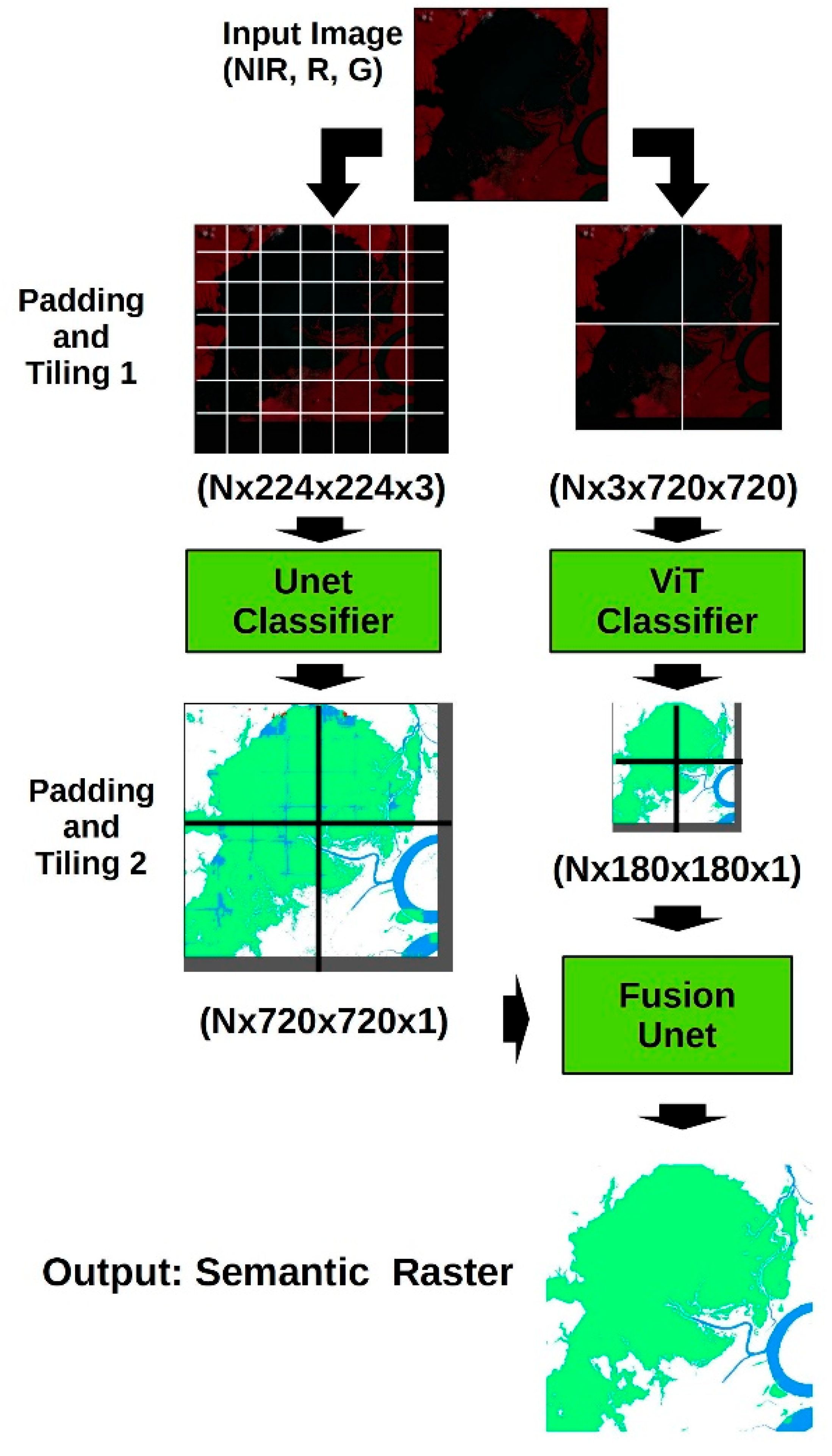
2.3. Model Architectures

We consider it outside of the remit of our work and expertise to develop new model architectures from scratch. Progress in deep learning is rapid, and as a result, Earth Observation practitioners have a wealth of architectures to choose from. From this perspective of Earth Observation, the challenge lies with the adaptation of algorithms often developed for medical imagery or computer vision to the specific challenges associated with satellite imagery (e.g., geocoding issues, multispectral imagery, the multiscalar nature of natural forms). In the general field of land-use classification related to water bodies, several authors have demonstrated that the combination of Unet and ViT architectures can deliver state-of-the-art results [22,23,24]. In medical imaging, the combination of attention Unets [15,25] and the Segformer Vision Transformer [26] is delivering state-of-the-art performance levels [24,25,26,27,28,29]. In the area of hydrology, the authors of [30] have demonstrated that the combination of Unets and the Segformer ViT can deliver a powerful segmentation performance level and produce an automated water level measurement workflow based solely on image data. We have therefore selected these 2 algorithms as the basis of our approach and propose to apply them, for the first time, to the problem of land-use classification at global scales. Specifically, we aim to deploy the attention-Unet on smaller image tiles in order to segment fine-grain features. Experience from [10] has taught us that the training performance for the river water and sediment bar classes tends to deteriorate as a function of tile size. This is likely due to the geometric properties river networks [31] which have a fractal dimension below 2. This means that as the area of the tile increases as the square of the width, the area of rivers within the tile increases at a slower rate and the overall proportion of rivers within a given tile decreases, thereby exacerbating class imbalance issues. This creates an impetus to use smaller tile sizes, which will have less overall spatial context, especially in the case of large rivers and lakes with a characteristic width larger than the tile dimension. We then aim to address this by deploying the Segformer ViT on larger tiles in order to encompass larger water bodies and give the classifier sufficient contextual shape information to distinguish large rivers from large lakes. The choice of 2 sizes of input tiles is intended to maximise the strengths and compensate for the weaknesses of each algorithm. We expect the Unet to make significant errors when a small input tile is mostly composed of surface water as it then becomes impossible, even for a human, to distinguish lakes from rivers in the absence of any context (e.g., a uniformly dark water image). Conversely, we expect the Segformer ViT to miss many small features given that the outputs have, by design, ¼ resolution of the inputs. The outputs of each algorithm are therefore expected to be complimentary, but we need to design a method of combining the semantic class rasters output from each algorithm and we choose a fusion approach. Image fusion is a well-researched topic [32,33,34,35]. However, in this particular case, our problem is made tractable by a number of simplifications with respect to many image fusion problems. First, we need to fuse single-channel semantic classification rasters with only 4 values representing our class categories (0 to 3 inclusively). Second, these rasters occupy the exact same spatial footprint thereby eliminating any need for co-registration. Third, we know the resolution differs exactly by a factor of 4, which is easy to incorporate in a Unet encoder pathway where XY dimensions typically halve at each layer following the max-pooling operation. We therefore propose a novel but straightforward dual-input Unet fusion approach which starts with the initial attention-Unet class raster at full resolution and then concatenates the ViT class raster as a second input after 2 layers of the encoder block, where the XY dimensions now at ¼ of the initial values. In the decoder pathway, we will again use attention gates in order to improve the detection of fine-grained details.

We implement the Unet classification architecture with code from [36] modified to (1) include a fourth encoder/decoder pair and (2) replace the upsampling layers in the decoder blocks with 2D transposed convolutions to perform the upsampling with trainable parameters. The architecture is designed for input images of 224 × 224 × 3 and is shown in Figure 2. Dimensions of 224 × 224 are somewhat arbitrary but convenient. In Sentinel-2 imagery, this equates to an image footprint of 2.24 km, which is larger than most (but not all) rivers [1]. Also, this is the common size used in many datasets, notably ImageNet [37], and makes the models and data produced here suitable for cross-comparisons and further research. Next, we use the TensorFlow [16] implementation of the Segformer B3 variant, pre-trained with the 1.2 million samples in the ImageNet-1K dataset [37], available in the Huggingface transformers Python package [38]. This architecture will be used on images of 720 × 720 × 3. These dimensions were arrived at after experimentation with our GPU and considerations of the scale of the world’s large water bodies. The Amazon river has a maximum width of roughly 3 km (300 pixels in Sentinel-2) [1]. Similarly for lakes, Downing et al. [2] estimate that of the ~300 million lakes on Earth, 15,905 have an area above 10 km². A tiles size of 720 × 720 @10 m, 51.8 km², should therefore sample the vast majority of terrestrial lakes. As stated above, our third model will be an image fusion algorithm that will combine the outputs of the classification attention-Unet, and the Segformer ViT is a modified attention-Unet with a dual input. We create a modified encoder block that concatenates the second input class raster at a point in the encoder pathway where the input raster has undergone 2 sets of convolutions and max pooling and therefore has XY dimensions of ¼ of the original input which matches the output of the ViT. Based on the success of the residual learning approach of [39], each encoder layer has a skip connection to the associated decoder layer in order to achieve the maximum retention of small features. The inputs dimensions are designed to be 720 × 720 × 1, obtained after re-assembling the tiles of 224 × 224 × 1 and re-splitting, and the 180 × 180 × 1 arrays directly output by the ViT. We refer to this as our Unet fusion model (Figure 3).

2.4. Training

We first train the semantic classification attention-Unet with the global pre-training data shown in Figure 1. Given that the pre-training data are produced from model outputs and post-processing filters, it has errors. Therefore, it is only used to prime the attention-Unet with a single epoch of training using sigmoid focal loss [40], and a learning rate of 10⁻⁵. We then use the 610 tiles of manually labelled seen data to create an fine-tuning set. We use the albumentations package [41] to create a total of 291,772 training samples and 31,284 validation samples. These are used to fine-tune the attention-Unet with an initial learning rate of 10⁻⁵, which halves at each epoch. We use sigmoid focal loss. The best weights were reached after 6 epochs of training, with a validation loss of 0.0033 and a validation accuracy of 0.9755. Next, we fine-tune the Segformer ViT. We again use our seen data and data augmentation to produce 144,648 training samples with an associated 16,164 validation samples. The Segformer ViT uses a custom loss function included in the model. With experimentation, we found that the validation loss stopped improving at a value of 0.073 after 8 epochs of training. Finally, we use both these models to produce training data for our dual-input Unet fusion model. We generated 127,777 training samples and 14,079 validation samples. We train the model with sigmoid focal loss and early stopping. The best weights were reached after 12 epochs, with a validation loss of 0.002 and a validation accuracy of 0.984.

2.5. Inference and Accuracy Assessment

Inference is performed by first processing the image in both the attention-Unet classifier and the ViT classifier. The respective semantic class raster outputs are then processed again with the fusion attention-Unet in order to produce the final semantic class raster. Figure 4 gives a summary of the inference pipeline. For the purpose of the quality assessment of the intermediary ViT classification outputs, which have ¼ of the initial image resolution, we perform a naive upsampling with a 4× repeat of each pixel. We assess the quality of the attention-Unet classifier, the ViT classifier and the attention-Unet fusion model (the final output) with the precision, recall and F1 scores calculated against the manually labelled masks.

3. Results

Figure 5 shows 3 examples chosen from the 67 seen testing tiles. The figure shows the image and the outputs from the attention-Unet, the Segformer ViT and the final class fusion model. The F1 scores show a weighted average for the river, lake and bar classes. We note the following key observations: The F1 score for the dual-input fusion model is higher than the intermediary F1 scores for either the attention-Unet or the ViT. The models display a strong ability to map rivers and lakes as distinct classes. Figure 6 shows 3 examples taken from the 100 unseen testing tiles. Here, we deliberately choose cases where significant errors in the attention-Unet outputs are recovered by the ViT. On the left, we see a case with a large lake. In this case, the attention-Unet output ambiguous results with many lake pixels falsely classified as river along the margins of several 224 × 224 tiles. The ViT did not make this error and produced a more consistent prediction. The final dual-input fusion prediction is more accurate than either the ViT or the attention-Unet. In the middle of Figure 6, we see a case where a wide river channel was falsely classified as a lake. Again, the ViT made a better prediction, and the fusion model is the most accurate. On the right of Figure 6, we see a case where a large area of dry land was falsely classified as dry river sediments. Once again, the ViT and final fused prediction did not inherit these errors.

In Figure 7, we show the distribution of F1 scores calculated for individual tiles in the seen and unseen test datasets. We use the Mann–Whitney U test and the Kolmogorov–Smirnov test to test for statistically significant differences in the distributions. For the seen data on the top of Figure 7, the Unet and ViT distributions are not significantly different with p-values of 0.208 and 0.329. The Unet and the Fusion distributions are significantly different with p-values of 0.013 and 0.016. Similarly, the ViT and Fusion distributions are significantly different with p-values < 0.000 in both cases. However, readers should note a tail of poor performance with a small number of samples having an f1 score below 0.6. In the case of the unseen data at the bottom of Figure 7, the Unet and ViT distributions are significantly different with p-values of 0.016 and 0.006. Here, the fusion distribution is very significantly different from both the Unet and ViT distribution with all paired tests returning p-values < 0.000. Again, there are some poorly performing outliers in the distribution. If we compare the fusion distributions for the seen and unseen data, we again find a significant difference with a p-value < 0.000. This confirms the slight degradation of performance in the unseen test data with respect to the seen test data.

Table 1. Precision, recall and F1 scores calculated for all pixels in all tiles of the seen and unseen test data. The seen testing data have 170 M pixels. Of these, 4.9 M are rivers, 10.0 M are lakes and 1.0 M are exposed sediment bars. The unseen data have 222 M pixels. Of these, 4.6 M are rivers, 10.5 M are lakes and 0.7 M are exposed sediment bars.

		Attention Unet Output			Segformer ViT Output			Fused Outputs
		Precision	Recall	F1	Precision	Recall	F1	Precision	Recall	F1
Seen	River	0.895	0.806	0.848	0.874	0.907	0.890	0.947	0.932	0.939
	Lake	0.876	0.947	0.910	0.908	0.950	0.929	0.955	0.972	0.963
	Bar	0.778	0.669	0.719	0.802	0.750	0.775	0.844	0.757	0.798
Unseen	River	0.819	0.712	0.762	0.822	0.894	0.857	0.927	0.913	0.920
	Lake	0.856	0.937	0.895	0.927	0.957	0.942	0.965	0.963	0.964
	Bar	0.372	0.588	0.456	0.685	0.780	0.729	0.734	0.781	0.757

presents the final aggregated results for both the seen and unseen test data. We give the precision, recall and F1 scores for the river class, the lake class and the exposed sediment bar class. The background class is omitted as it always gives results in excess of 0.98, which is a high value not representative of the actual errors in the classes of interest. Overall, these results show that the ViT tends to slightly outperform the attention-Unet. This is most acute in the unseen data where the ViT outperforms the attention-Unet by 9%, 7% and 28% for rivers, lakes and bars, respectively. This does not contradict the results in Figure 7. When we calculate a single F1 score for all the individual pixels in the datasets, the low-performing outliers in Figure 7 have a large impact. Table 1 also shows that all scores are systematically best for the fused predictions. In terms of F1 scores, the fused model improves on the ViT model by 2–6 %. Table 1 also shows that the results have slightly deteriorated when we compare seen and unseen data with an F1 score degradation of 2% and 4% for rivers and bars (respectively), while the lake performance level has remained stable to within 0.1%.

4. Discussion

The attention-Unet and the Segformer ViT delivered complimentary performance levels. The attention-Unet delivered fine-grained predictions that were mostly very accurate but somewhat prone to catastrophic failures (Figure 6 and Figure 7). The Segformer ViT was computationally efficient and delivered a robust performance level much less prone to failures, but its best outputs were often of slightly lower quality than the attention-Unet (Figure 6 and Figure 7). A novel yet straightforward dual-input image fusion model that fuses both semantic classification rasters was found to effectively learn rules to optimally combine these outputs and use ViT results to recover the errors of the attention-Unet classifier while keeping the native resolution of the input imagery (here, 10 m). This delivered the best results and made predictions that were better than either the attention-Unet or the Segformer ViT. Importantly, our results suffer only a minor but statistically significant degradation when the pipeline is applied to the unseen data. We see evidence in Figure 7 that the pre-training of the attention-Unet on a comprehensive dataset of 2.1 million samples evenly spread across the globe did make it robust when applied to the unseen data. In the seen data, the distributions for the Unet and ViT are not significantly different. But in the case of the unseen data, the ViT performance is weaker than that of the Unet with a statistically significant difference in distributions (p < 0.000). This suggests that whilst large pretrained models developed for computer science applications have significant potential for Earth Observation, features learned from training on images not related to Earth Observation are not perfectly transferable. Finally, our final classification results are delivered without the need for intensive post-processing, which overcompensates for the fact that we now need to run 3 models instead of the single model of [10].

Drawing a comparison with other works is constrained by the fact that there are very few other published works that report on the specific task of classifying rivers as a distinct semantic class at global scales. The nearest comparator is [10]. With the use of post-processing filters, the authors report recalls of 95%, 94% and 61% for rivers, lakes and bars, respectively, and precisions of 92%, 84% and 84% for rivers, lakes and bars, respectively. Without these post-processing filters, the authors report recalls of 56%, 95% and 57% for rivers, lakes and bars, and precisions of 88%, 73% and 84% for rivers, lakes and bars, respectively. The results presented here, all achieved without post-processing, are a marked improvement. In another work, Nyberg et al. [13] report on a global analysis of river channel belts based a fully convolutional network using VGG-19 as a backbone applied to global Landsat data. They do not report F1 scores or other similar metrics but they report a final sparse categorical cross entropy loss of 0.15 on their validation data with an accuracy of 94% for a binary river/non-river problem. For our seen test data, the sparse categorical cross-entropy (scc) is 0.15 and the accuracy is 99%. The SCC loss is 0.11 with an accuracy 99% for the unseen test data. The DeepWaterV2 model, ref. [42] only classifies freshwater based on Landsat data. They report an F1 score of 0.91 for their water class. The ESA Worldcover product has a water body class with an estimated F1 score of 0.87 [6]. Additionally, the authors of [9] classify open water based on Sentinel-1 and Sentinel-2 input imagery. In the case of Sentinel-2 imagery, they find a best F1 score of 0.96. Finally, the Dynamic World product of [7] has a water body class with an F1 score of 0.98. When we merge our river and lake classes, we obtain an F1 score for the new freshwater class of 0.97 and 0.96 for seen and unseen test data, respectively. This value is comparable to other global scale surveys reported above. At smaller scales, the authors of [43] tested a range of models, including Vision Transformers, on several local-scale benchmark datasets located in China. They also found that the attention-based SWIN-Unet performs best with a reported accuracy of 0.96 for a freshwater class that merges rivers and lakes.

5. Conclusions

We have presented a deep learning pipeline capable of classifying rivers as a distinct semantic class and which can be deployed at global scales with state-of-the-art results. As a preliminary test of global deployment, we have run the pipeline on an area of 12 × 14 degrees (11.6 gigapixels per channel) centred around Italy. Inference required ~90 min for a given time period. Extrapolated to a global area, this suggests that processing a full classification for the non-polar world (approximately 2 terapixels per channel) at a resolution of 10 metres would now require ~10 days. This is three times faster than the pipeline of [10] and brings into reach multi-seasonal and multi-annual monitoring for all the major rivers of the world.

References

1. Downing, J.; Cole, J.; Duarte, C.; Middelburg, J.; Melack, J.; Prairie, Y.; Kortelainen, P.; Striegl, R.; McDowell, W.; Tranvik, L. Global abundance and size distribution of streams and rivers. Inland Waters 2012, 2, 229–236. [Google Scholar] [CrossRef]
2. Downing, J.A.; Prairie, Y.T.; Cole, J.J.; Duarte, C.M.; Tranvik, L.J.; Striegl, R.G.; McDowell, W.H.; Kortelainen, P.; Caraco, N.F.; Melack, J.M.; et al. The global abundance and size distribution of lakes, ponds, and impoundments. Limnol. Oceanogr. 2006, 51, 2388–2397. [Google Scholar] [CrossRef]
3. Vörösmarty, C.J.; McIntyre, P.B.; Gessner, M.O.; Dudgeon, D.; Prusevich, A.; Green, P.; Glidden, S.; Bunn, S.E.; Sullivan, C.A.; Liermann, C.R.; et al. Global threats to human water security and river biodiversity. Nature 2010, 467, 555–561. [Google Scholar] [CrossRef]
4. Dudgeon, D.; Arthington, A.H.; Gessner, M.O.; Kawabata, Z.-I.; Knowler, D.J.; Lévêque, C.; Naiman, R.J.; Prieur-Richard, A.-H.; Soto, D.; Stiassny, M.L.J.; et al. Freshwater biodiversity: Importance, threats, status and conservation challenges. Biol. Rev. 2006, 81, 163–182. [Google Scholar] [CrossRef]
5. Tockner, K.; Stanford, J.A. Riverine flood plains: Present state and future trends. Environ. Conserv. 2002, 29, 308–330. [Google Scholar] [CrossRef]
6. Zanaga, D.; Van De Kerchove, R.; Daems, D.; De Keersmaecker, W.; Brockmann, C.; Kirches, G.; Wevers, J.; Cartus, O.; Santoro, M.; Fritz, S.; et al. ESA WorldCover 10 m 2021 V200 2022. Available online: https://developers.google.com/earth-engine/datasets/catalog/ESA_WorldCover_v200 (accessed on 1 July 2024).
7. Brown, C.F.; Brumby, S.P.; Guzder-Williams, B.; Birch, T.; Hyde, S.B.; Mazzariello, J.; Czerwinski, W.; Pasquarella, V.J.; Haertel, R.; Ilyushchenko, S.; et al. Dynamic World, Near real-time global 10 m land use land cover mapping. Sci. Data 2022, 9, 251. [Google Scholar] [CrossRef]
8. Pekel, J.-F.; Cottam, A.; Gorelick, N.; Belward, A.S. High-resolution mapping of global surface water and its long-term changes. Nature 2016, 540, 418–422. [Google Scholar] [CrossRef]
9. Wieland, M.; Fichtner, F.; Martinis, S.; Groth, S.; Krullikowski, C.; Plank, S.; Motagh, M. S1S2-Water: A Global Dataset for Semantic Segmentation of Water Bodies from Sentinel-1 and Sentinel-2 Satellite Images. IEEE J. Sel. Top. Appl. Earth Obs. Remote Sens. 2023, 17, 1084–1099. [Google Scholar] [CrossRef]
10. Carbonneau, P.E.; Bizzi, S. Global mapping of river sediment bars. Earth Surf. Process. Landf. 2023, 49, 15–23. [Google Scholar] [CrossRef]
11. Allen, G.H.; Pavelsky, T.M. Global extent of rivers and streams. Science 2018, 361, 585–588. [Google Scholar] [CrossRef]
12. Dallaire, C.O.; Lehner, B.; Sayre, R.; Thieme, M. A multidisciplinary framework to derive global river reach classifications at high spatial resolution. Environ. Res. Lett. 2019, 14, 024003. [Google Scholar] [CrossRef]
13. Nyberg, B.; Henstra, G.; Gawthorpe, R.L.; Ravnås, R.; Ahokas, J. Global scale analysis on the extent of river channel belts. Nat. Commun. 2023, 14, 2163. [Google Scholar] [CrossRef] [PubMed]
14. Lehner, B.; Verdin, K.; Jarvis, A. New Global Hydrography Derived from Spaceborne Elevation Data. Eos Trans. Am. Geophys. Union 2008, 89, 93–94. [Google Scholar] [CrossRef]
15. Oktay, O.; Schlemper, J.; Folgoc, L.L.; Lee, M.; Heinrich, M.; Misawa, K.; Mori, K.; McDonagh, S.; Hammerla, N.Y.; Kainz, B.; et al. Attention U-Net: Learning Where to Look for the Pancreas. arXiv 2018, arXiv:1804.03999. [Google Scholar]
16. Abadi, M.; Agarwal, A.; Barham, P.; Brevdo, E.; Chen, Z.; Citro, C.; Corrado, G.S.; Davis, A.; Dean, J.; Devin, M.; et al. TensorFlow: Large-Scale Machine Learning on Heterogeneous Distributed Systems. arXiv 2016, arXiv:1603.04467v2. [Google Scholar]
17. Pedregosa, F.; Varoquaux, G.; Gramfort, A.; Michel, V.; Thirion, B.; Grisel, O.; Blondel, M.; Prettenhofer, P.; Weiss, R.; Dubourg, V.; et al. Scikit-Learn: Machine Learning in Python. J. Mach. Learn. Res. 2011, 12, 2825–2830. [Google Scholar]
18. van der Walt, S.; Schönberger, J.L.; Nunez-Iglesias, J.; Boulogne, F.; Warner, J.D.; Yager, N.; Gouillart, E.; Yu, T. Scikit-Image: Image Processing in Python. PeerJ 2014, 2, e453. [Google Scholar] [CrossRef]
19. Virtanen, P.; Gommers, R.; Oliphant, T.E.; Haberland, M.; Reddy, T.; Cournapeau, D.; Burovski, E.; Peterson, P.; Weckesser, W.; Bright, J.; et al. SciPy 1.0: Fundamental Algorithms for Scientific Computing in Python. Nat. Methods 2020, 17, 261–272. [Google Scholar] [CrossRef]
20. GDAL Dev. Team GDAL—Geospatial Data Abstraction Library; GD Arabia Ltd.: Riyadh, Saudi Arabia, 2018. [Google Scholar]
21. Carbonneau, P.; Bizzi, S. Seasonal Monitoring of River and Lake Water Surface Areas at Global Scale with Deep Learning. 2022. Available online: https://assets-eu.researchsquare.com/files/rs-2254580/v2_covered.pdf?c=1670341515 (accessed on 1 July 2024).
22. Zhou, N.; Xu, M.; Shen, B.; Hou, K.; Liu, S.; Sheng, H.; Liu, Y.; Wan, J. ViT-UNet: A Vision Transformer Based UNet Model for Coastal Wetland Classification Based on High Spatial Resolution Imagery. IEEE J. Sel. Top. Appl. Earth Obs. Remote Sens. 2024, 17, 19575–19587. [Google Scholar] [CrossRef]
23. Tong, Q.; Wu, J.; Zhu, Z.; Zhang, M.; Xing, H. STIRUnet: SwinTransformer and Inverted Residual Convolution Embedding in Unet for Sea–Land Segmentation. J. Environ. Manag. 2024, 357, 120773. [Google Scholar] [CrossRef]
24. Zhao, X.; Wang, H.; Liu, L.; Zhang, Y.; Liu, J.; Qu, T.; Tian, H.; Lu, Y. A Method for Extracting Lake Water Using ViTenc-UNet: Taking Typical Lakes on the Qinghai-Tibet Plateau as Examples. Remote Sens. 2023, 15, 4047. [Google Scholar] [CrossRef]
25. Vaswani, A.; Shazeer, N.; Parmar, N.; Uszkoreit, J.; Jones, L.; Gomez, A.N.; Kaiser, L.; Polosukhin, I. Attention Is All You Need. In Proceedings of the Advances in Neural Information Processing Systems 30 (NIPS 2017), Long Beach, CA, USA, 4–9 December 2017. [Google Scholar]
26. Xie, E.; Wang, W.; Yu, Z.; Anandkumar, A.; Alvarez, J.M.; Luo, P. SegFormer: Simple and Efficient Design for Semantic Segmentation with Transformers. In Proceedings of the Advances in Neural Information Processing Systems 34 (NeurIPS 2021), Virtual, 6–14 December 2021. [Google Scholar]
27. Wang, F.; Silvestre, G.; Curran, K. MiTU-Net: A Fine-Tuned U-Net with SegFormer Backbone for Segmenting Pubic Symphysis-Fetal Head. arXiv 2024, arXiv:2401.15513. [Google Scholar]
28. Yeom, S.-K.; von Klitzing, J. U-MixFormer: UNet-like Transformer with Mix-Attention for Efficient Semantic Segmentation. arXiv 2023, arXiv:2312.06272. [Google Scholar]
29. Chen, J.; Lu, Y.; Yu, Q.; Luo, X.; Adeli, E.; Wang, Y.; Lu, L.; Yuille, A.L.; Zhou, Y. TransUNet: Transformers Make Strong Encoders for Medical Image Segmentation. arXiv 2021, arXiv:2102.04306. [Google Scholar]
30. Xie, Z.; Jin, J.; Wang, J.; Zhang, R.; Li, S. Application of Deep Learning Techniques in Water Level Measurement: Combining Improved SegFormer-UNet Model with Virtual Water Gauge. Appl. Sci. 2023, 13, 5614. [Google Scholar] [CrossRef]
31. Tarboton, D.G.; Bras, R.L.; Rodriguez-Iturbe, I. The Fractal Nature of River Networks. Water Resour. Res. 1988, 24, 1317–1322. [Google Scholar] [CrossRef]
32. Ghassemian, H. A Review of Remote Sensing Image Fusion Methods. Inf. Fusion 2016, 32, 75–89. [Google Scholar] [CrossRef]
33. Choudhary, G.; Sethi, D. From Conventional Approach to Machine Learning and Deep Learning Approach: An Experimental and Comprehensive Review of Image Fusion Techniques. Arch. Comput. Methods Eng. 2023, 30, 1267–1304. [Google Scholar] [CrossRef]
34. Smikrud, K.M.; Prakash, A.; Nichols, J.V. Decision-Based Fusion for Improved Fluvial Landscape Classification Using Digital Aerial Photographs and Forward Looking Infrared Images. Photogramm. Eng. Remote Sens. 2008, 74, 903–911. [Google Scholar] [CrossRef]
35. Zhang, Y.; Chi, M. Mask-R-FCN: A Deep Fusion Network for Semantic Segmentation. IEEE Access 2020, 8, 155753–155765. [Google Scholar] [CrossRef]
36. Tomar, N. Nikhilroxtomar/Semantic-Segmentation-Architecture 2024. Available online: https://github.com/nikhilroxtomar/Semantic-Segmentation-Architecture (accessed on 1 July 2024).
37. Deng, J.; Dong, W.; Socher, R.; Li, L.-J.; Li, K.; Li, F.-F. ImageNet: A Large-Scale Hierarchical Image Database. In Proceedings of the 2009 IEEE Conference on Computer Vision and Pattern Recognition, Miami, FL, USA, 20–25 June 2009. [Google Scholar] [CrossRef]
38. HuggingFace, H. Transformers: State-of-the-Art Machine Learning for JAX, PyTorch and TensorFlow 2024. Available online: https://github.com/huggingface/transformers (accessed on 1 July 2024).
39. He, K.; Zhang, X.; Ren, S.; Sun, J. Deep Residual Learning for Image Recognition. In Proceedings of the 2016 IEEE Conference on Computer Vision and Pattern Recognition (CVPR), Las Vegas, NV, USA, 27–30 June 2016; pp. 770–778. [Google Scholar]
40. Lin, T.-Y.; Goyal, P.; Girshick, R.; He, K.; Dollár, P. Focal Loss for Dense Object Detection. IEEE Trans. Pattern Anal. Mach. Intell. 2020, 42, 318–327. [Google Scholar] [CrossRef] [PubMed]
41. Buslaev, A.; Iglovikov, V.I.; Khvedchenya, E.; Parinov, A.; Druzhinin, M.; Kalinin, A.A. Albumentations: Fast and Flexible Image Augmentations. Information 2020, 11, 125. [Google Scholar] [CrossRef]
42. Isikdogan, L.F.; Bovik, A.; Passalacqua, P. Seeing Through the Clouds with DeepWaterMap. IEEE Geosci. Remote Sens. Lett. 2020, 17, 1662–1666. [Google Scholar] [CrossRef]
43. Hao, M.; Dong, X.; Jiang, D.; Yu, X.; Ding, F.; Zhuo, J. Land-Use Classification Based on High-Resolution Remote Sensing Imagery and Deep Learning Models. PLoS ONE 2024, 19, e0300473. [Google Scholar] [CrossRef]
44. Carbonneau, P.E. Global Scale Attention-Based Deep Learning for River Landscape Classification [Dataset]; Durham University: Durham, UK, 2024. [Google Scholar]
Figure 1. Study area covering 89% of the Earth’s surface. Markers show the location of manually labelled samples of 0.15° × 0.15°, (~15 × 15 km). Seen data were used for training, validation and testing. Unseen data are spatially distinct from the seen data and was only used for testing. Graduated background shows the number of pre-training data samples extracted from modelled results for each 5° × 5° grid cell.
Remotesensing 16 04747 g001
Figure 2. Semantic classification attention-Unet architecture with a 3-channel input and a 4-class softmax output. Dimensions are given for the outputs of each layer. Decoder blocks include an attention gate that performs additive attention as per [15]. Total trainable parameters: 21.6 million.
Remotesensing 16 04747 g002
Figure 3. Dual-input fusion attention-Unet architecture. First input is the semantic class raster of 720 × 720 × 1 produced by the attention-Unet. The second input of 180 × 180 × 1 has ¼ of the resolution, occupies the same spatial footprint and is produced by the Segformer ViT. It is concatenated to the features after the first input has been downsampled by a factor of 4. A skip connection is added from the first input to the final decoder output to re-enforce the presence of high-resolution, fine-grained features. Total trainable parameters: 2.2 million.
Remotesensing 16 04747 g003
Figure 4. Inference flow chart showing the full pipeline.
Remotesensing 16 04747 g004
Figure 5. Seen data classification examples. Top row shows the initial image. Successive rows show the attention-Unet classification, the Segformer ViT classification and the fused output. Rivers are in blue, lakes in green and exposed sediment bars in red. F1 scores are the pixel-weighted average of F1 scores for the river class, the lake class and the sediment bar class. Scale bars on the bottom right of each column represent 10 km.
Remotesensing 16 04747 g005
Figure 6. Error recovery examples for Unseen data classification where Unet errors are recovered by the ViT and subsequent fusion. Top row shows the initial image. Successive rows show the attention-Unet classification, the Segformer ViT classification and the fused output. Legend and scale bars are as in Figure 5.
Remotesensing 16 04747 g006
Figure 7. Distributions of pixel-weighted average F1 scores of the river, lake and sediment bar classes calculated for individual test tiles with respect to manual labelled ground truth masks.
Remotesensing 16 04747 g007