Color-Distortion Correction for Jilin-1 KF01 Series Satellite Imagery Using a Data-Driven Method

Abstract

Color distortion is a common issue in Jilin-1 KF01 series satellite imagery, a phenomenon caused by the instability of the sensor during the imaging process. In this paper, we propose a data-driven method to correct color distortion in Jilin-1 KF01 imagery. Our method involves three key aspects: color-distortion simulation, model design, and post-processing refinement. First, we investigate the causes of color distortion and propose algorithms to simulate this phenomenon. By superimposing simulated color-distortion patterns onto clean images, we construct color-distortion datasets comprising a large number of paired images (distorted–clean) for model training. Next, we analyze the principles behind a denoising model and explore its feasibility for color-distortion correction. Based on this analysis, we train the denoising model from scratch using the color-distortion datasets and successfully adapt it to the task of color-distortion correction in Jilin-1 KF01 imagery. Finally, we propose a novel post-processing algorithm to remove boundary artifacts caused by block-wise image processing, ensuring consistency and quality across the entire image. Experimental results show that the proposed method significantly eliminates color distortion and enhances the radiometric quality of Jilin-1 KF01 series satellite imagery, offering a solution for improving its usability in remote sensing applications.

1. Introduction

Optical remote sensing satellites provide an abundance of optical imagery of the Earth’s surface, one which is widely used in research fields such as geology, environmental science, and agriculture, as well as in practical applications like natural resource management, urban planning, and disaster monitoring [1,2,3,4,5,6]. However, due to limitations in satellite imaging systems and the influence of external environmental factors during the imaging process, different detector elements within the same sensor may respond inconsistently to the same radiative energy, resulting in stripe noise in the imagery [7]. Stripe noise not only degrades the radiometric quality of remote sensing images but also affects their usability.

Over the past few decades, researchers have extensively studied methods for removing stripe noise and have proposed a variety of approaches which can be broadly categorized into three types: statistical-based methods, filtering-based methods, and optimization-based methods. Statistical-based methods include histogram matching [8,9,10,11] and moment matching [12,13,14,15]. Histogram matching removes stripe noise by adjusting the gray level distribution of the original image to match a target distribution, while moment matching achieves noise reduction by adjusting the mean and variance of the original image to align with reference values. Filtering-based methods include the Fourier transform [16,17] and wavelet transform [18,19,20]. The Fourier transform converts the original image from the spatial domain to the frequency domain, in which the frequency components associated with stripe noise are removed, before converting the image back to the spatial domain, resulting in a noise-free image. The wavelet transform separates stripe noise from signals at different scales and then filters out the stripe noise to obtain a clean image. Optimization-based methods treat stripe noise removal as an ill-posed optimization problem [21], utilizing prior knowledge such as total variation [22], sparsity [23], and low-rank properties [24] to solve it. Since satellite images are acquired in a push-broom manner, the stripe noise typically exhibits a unidirectional characteristic along the satellite’s orbital direction; therefore, Bouali and Ladjal introduced a unidirectional total variation model [22], and subsequent researchers have proposed spatially weighted regularization terms to enhance the adaptability of the total variation model [25,26]. Liu et al. used $l_0$-norm-based regularization to represent the global sparsity of stripe noise, achieving its removal by separating the stripe components [23]. He and Zhang leveraged the low-rank characteristic of hyperspectral images and matrix decomposition theory to remove stripe noise [27,28,29].

The Jilin-1 KF01 series satellites offer the advantages of high resolution and broad width, but their imagery products also exhibit stripe noise. Filtering-based methods may remove useful signals along with the stripe noise, while optimization-based methods are often dependent on prior knowledge and involve complex models, resulting in inefficiencies and limitations in practical applications. Therefore, the Jilin-1 KF01 series satellites employ histogram matching, a statistically based method, to remove stripe noise. Histogram matching effectively eliminates high-frequency stripe noise in the imagery; however, low-frequency stripe noise may still persist, as shown in Figure 1. Figure 1a shows the image before histogram matching, when both the high-frequency and the low-frequency stripe noise are present. Figure 1b shows the image after histogram matching, when the high-frequency stripe noise has been removed, but low-frequency stripe noise remains. These low-frequency stripes, which vertically traverse the entire image with relatively broad widths, are referred to as “color distortion” in the following sections of this paper. The Jilin-1 KF01 series satellites capture a large volume of remote sensing imagery daily. However, existing methods fail to effectively address the issue of color distortion in these images. The presence of color distortion significantly degrades the radiometric quality of the imagery, rendering it unsuitable for direct use and adversely affecting the production of advanced remote sensing imagery products. Therefore, there is an urgent need for a new method to resolve the color-distortion problem in Jilin-1 KF01 satellite imagery.

In recent years, deep learning-based methods have been increasingly applied to remote sensing imagery processing tasks, such as denoising [30,31,32,33], super-resolution [34,35,36,37], and destriping [38,39,40,41,42,43], due to their powerful learning capabilities. These deep learning-based destriping algorithms perform well in removing high-frequency stripe noise but are less effective in addressing color distortion. This is mainly due to the way training datasets are constructed. In remote sensing imagery, it is challenging to obtain both images with real stripe noise and their corresponding clean images. As a result, the stripes need to be simulated. A common approach is to add zero-mean Gaussian white noise to each column of the clean image, band by band, to generate corresponding images with stripe noise [39,40,41]. While this method can effectively simulate high-frequency stripe noise, it fails to simulate color distortion. Consequently, models trained on such datasets are unable to solve color distortion.

To address the issue of color distortion in the imagery of the Jilin-1 KF01 series satellites, we conducted research from three key aspects: color-distortion simulation, model design, and post-processing refinement. First, we performed an in-depth analysis of the causes of color distortion in the Jilin-1 KF01 series satellite imagery and developed algorithms to simulate the color distortion. By adding simulated color-distortion patterns to clean images, we were able to generate corresponding distorted images, allowing us to construct color-distortion datasets containing a large number of paired images (distorted image–clean image) for training the model. In terms of the model, we employed a denoising model from the field of computer vision which was originally designed for handling Gaussian noise; we retrained this denoising model from scratch using the color-distortion datasets, achieving excellent results in the color-distortion correction task. Since the individual images are quite large and need to be processed in blocks, simply setting overlapping regions between blocks was not sufficient to remove boundary artifacts; therefore, we developed a specialized post-processing algorithm to remove boundary artifacts caused by block-wise processing.

In summary, our contributions include the following:

• We conducted a thorough analysis of the causes of color distortion (i.e., low-frequency stripe noise) in Jilin-1 KF01 imagery and developed algorithms to simulate this distortion. To the best of our knowledge, this is the first work in the field of remote sensing imagery processing to simulate color distortion. For the color distortion in the Jilin-1 KF01 series satellite imagery, our algorithms have shown excellent simulation performance.
• We analyzed the underlying similarities between the principles of a denoising model and those of the color-distortion correction model. With this analysis as a foundation, we successfully adapted a denoising model originally used in the field of computer vision for the task of color-distortion correction in Jilin-1 KF01 imagery.
• To address the boundary artifacts caused by block-wise processing of large-size images, we proposed a post-processing algorithm. This algorithm effectively removes boundary artifacts and ensures an overall consistency between image blocks, significantly improving the processing results of large-size images.

2. Methods

The aim of this study is to eliminate the residual color-distortion in the BGR bands of Jilin-1 KF01 series satellite imagery after histogram matching. This section provides an in-depth analysis of the causes of residual color-distortion and details the simulation of the distortion and the principles behind the color-distortion correction model, as well as the design of the post-processing algorithm.

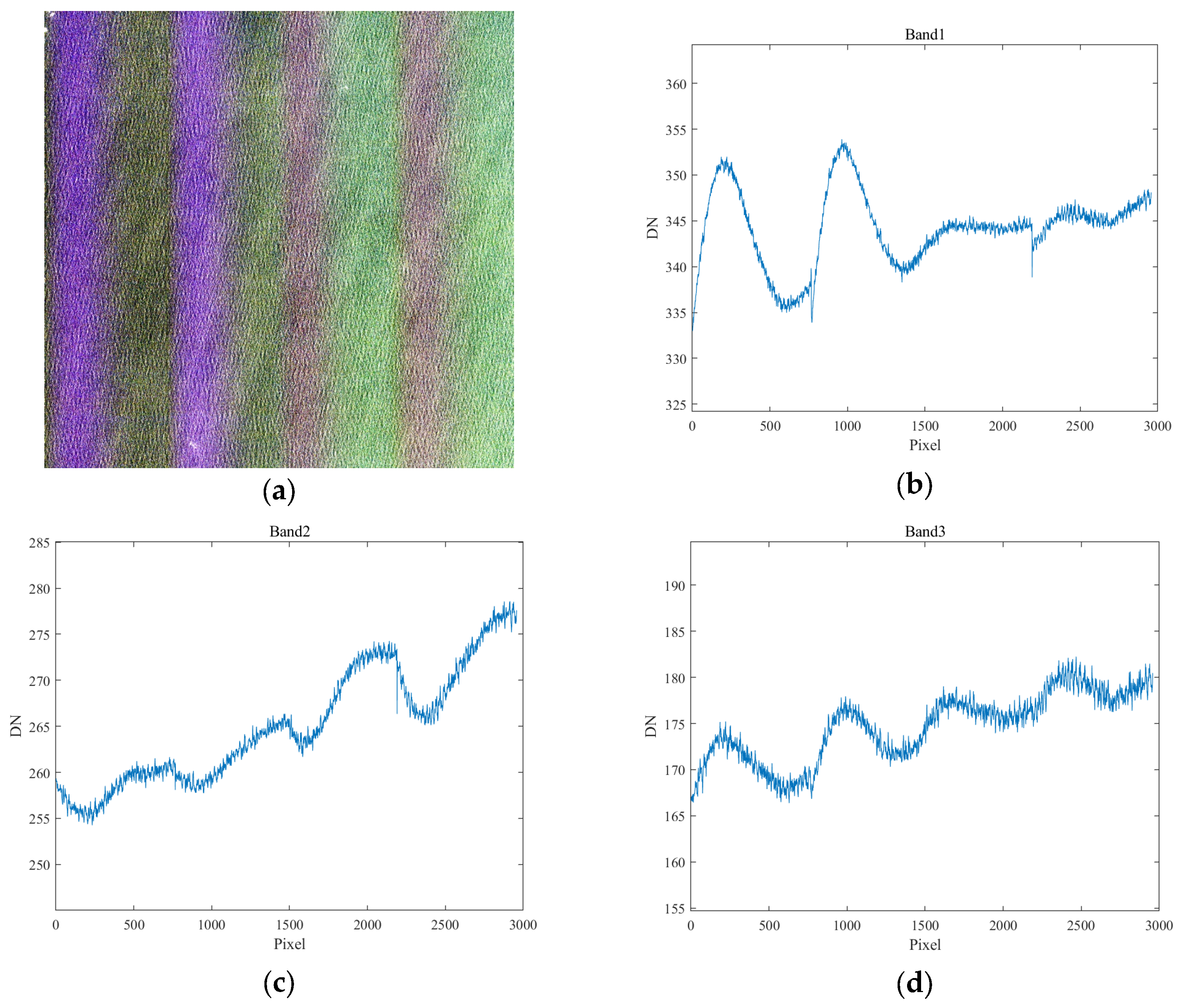
2.1. Causes of Residual Color-Distortion

To identify the causes of residual color-distortion, we first analyzed laboratory calibration images. Figure 2a shows an original calibration image of the Band 1 spectral band from a Jilin-1 KF01 CCD line-scan sensor, and different rows in the calibration image represent calibration data at various times. Vertical high-frequency stripe noise and color distortion are visible in the image. After applying laboratory calibration coefficients, the corrected result is shown in Figure 2b, where the high-frequency stripe noise has largely disappeared. The column-wise mean of the corrected calibration image (i.e., Figure 2b) is presented in Figure 2c, demonstrating that although color distortion is significantly reduced, it still persists. We computed the column-wise standard deviation for the original calibration image (i.e., Figure 2a), with the results shown in Figure 2d. The non-zero standard deviation indicates that the rows in Figure 2a are not completely identical, suggesting sensor instability during the imaging process. These slight variations in the calibration data over time prevent the laboratory calibration coefficients from fully correcting each row of the original calibration image, resulting in residual color-distortion.

We also analyzed remote sensing images transmitted by the Jilin-1 KF01 series satellites after they entered orbit. Three sea scenes captured by the same camera during a single imaging task were selected at regular intervals, as indicated by the red boxes in Figure 3a. Focusing on the Band 1 spectral band of these three scenes, we subtracted the mean from each scene and then computed the column-wise mean; this can significantly reduce interference from ground features, allowing us to better observe the color-distortion pattern itself. Figure 3b shows the resulting color-distortion patterns derived using this method, where “DN” (Digital Number) represents the quantized value of the radiation received by the sensor. As seen in Figure 3b, the color-distortion pattern changes over time within the same imaging task (differences in color-distortion patterns between scenes are highlighted by the green elliptical areas in Figure 3b); these variations lead to instability in relative radiometric correction, resulting in residual color-distortion.

Based on the above analysis, it is clear that the instability in the sensor during the imaging process affects the correction results, leading to residual color-distortion. The method proposed in this paper effectively addresses this issue.

2.2. Image Degradation Model

Color distortion is a common issue in Jilin-1 KF01 imagery, in which the color distortion is distributed along the orbital direction. Within a single scene, the same column in the image can be considered to be affected by the same color distortion. Assuming the color distortion is additive noise, the image degradation model can be expressed as shown in Formula (1):

$$\mathit{K}=\mathit{I}+\mathit{N},$$

(1)

where $\mathit{K}\in {\mathbb{R}}^{b\times h\times w}$ represents the degraded image with color distortion, $\mathit{I}\in {\mathbb{R}}^{b\times h\times w}$ denotes the clean image, and $\mathit{N}\in {\mathbb{R}}^{b\times h\times w}$ represents the color-distortion pattern. The variables $b,h$, and $w$ correspond to the number of spectral bands, image height, and image width, respectively. The goal of the color-distortion correction task is to recover the clean image $\mathit{I}$ from the distorted image $\mathit{K}$.

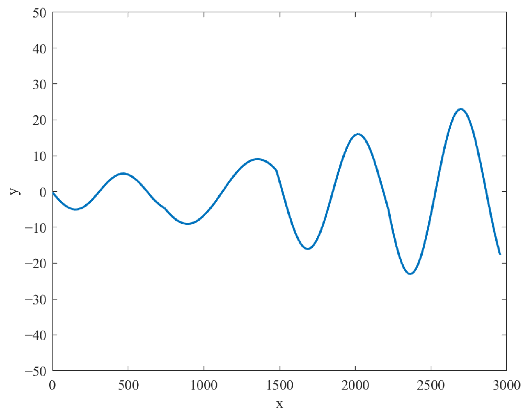
2.3. Color-Distortion Simulation

To train a color-distortion correction model, we need to construct datasets containing a large number of paired images (distorted images–clean images). For remote sensing imagery, it is often difficult to obtain such paired data directly. Previous research works have simulated stripe noise using Gaussian white noise, but this approach only simulates high-frequency stripe noise and cannot simulate color distortion. Therefore, we analyzed the Jilin-1 KF01’s laboratory calibration images and remote sensing images transmitted after the Jilin-1 KF01 series satellites were in orbit, and designed algorithms to simulate the color-distortion pattern.

Some of the laboratory calibration images from the Jilin-1 KF01 series satellites are shown in Figure 4. Figure 4a displays the original laboratory calibration images of the CCD sensor’s Band 1-to-Band 3 spectral bands (i.e., BGR bands). The column-wise mean of each band was calculated, and the results are shown in Figure 4b. From Figure 4b, it can be seen that the color-distortion patterns of the Jilin-1 KF01 series satellites closely resemble sine functions.

When analyzing the color-distortion patterns in satellite-transmitted remote sensing images, it is necessary to select a uniform ground to minimize the influence of ground features on the color-distortion patterns. In this analysis, we used sea imagery and calculated the column-wise mean values of the BGR bands. As shown in Figure 5, color distortion is present in all three spectral bands, and the distortion patterns also resemble sine functions.

Based on the analysis of laboratory calibration images and satellite-transmitted remote sensing images, we used sine functions to simulate the color-distortion patterns in individual spectral bands of a single image. The color-distortion patterns added to each spectral band are independent of one another. The function for generating a color-distortion pattern for a single spectral band in an image is shown in Formula (2):

$$y=\left\{\begin{array}{l}{A}_1\sin \left({\omega }_{1}x+{\phi }_1\right),0\le x<n\\ A_2\sin \left({\omega }_{2}x+{\phi }_2\right),n\le x<2n\\ A_3\sin \left({\omega }_{3}x+{\phi }_3\right),2n\le x<3n\\ A_4\sin \left({\omega }_{4}x+{\phi }_4\right),3n\le x<4n\end{array}\right.,$$

(2)

where $A_i$, ${\omega }_i$, and ${\phi }_i$($i=1,2,3,4$) represent the amplitude, angular frequency, and initial phase of the sine function, respectively, and $n$ refers to a quarter of the width of a remote sensing image. Based on our observations of the color-distortion patterns in multiple Jilin-1 KF01 images, we set the amplitude $A_i$ as a random number $\left[1,\right.\left.25\right)$. For ${\omega }_i$, we first choose the period $T_i$ as a random number in the range $\left({\displaystyle \frac{n}{1.25}},\left.{\displaystyle \frac{n}{0.25}}\right]\right.$, and according to ${\omega }_i={\displaystyle \frac{2\pi }{T_i}}$, ${\omega }_i$ is set as a random number between $\left[{\displaystyle \frac{0.5\pi }{n}},\left.{\displaystyle \frac{2.5\pi }{n}}\right)\right.$. To determine the value of ${\phi }_i$, we ensured that the function values of adjacent sine functions at the connection points were equal and that the first-order derivatives at those points had the same sign. Initially, we set ${\phi }_1$ as a random number in the interval $\left[0,\left.T_1{\omega }_1\right)\right.$; at $x=n,$ the following relationship holds:

$$A_1\sin \left({\omega }_{1}n+{\phi }_1\right)=A_2\sin \left({\omega }_{2}n+{\phi }_2\right),$$

(3)

$$A_1{\omega }_1\cos \left({\omega }_{1}n+{\phi }_1\right) \times A_2{\omega }_2\cos \left({\omega }_{2}n+{\phi }_2\right)\ge 0.$$

(4)

According to Formula (3), it can be derived that

$${\phi }_2=\arcsin \left({\displaystyle \frac{A_1\sin \left({\omega }_{1}n+{\phi }_1\right)}{A_2}}\right)-{\omega }_{2}n,$$

(5)

and due to the symmetry of the sine function, the value of ${\phi }_2$ is not unique; the other solution of ${\phi }_2$, denoted as ${\phi }_2^{\prime }$, is given as follows:

$${\phi }_2^{\prime }=\mathsf{\pi }-\arcsin \left({\displaystyle \frac{A_1\sin \left({\omega }_{1}n+{\phi }_1\right)}{A_2}}\right)-{\omega }_{2}n.$$

(6)

According to Formula (4), the unique solution for ${\phi }_2$ that meets the required conditions can be selected from the two possible solutions. Using the same approach, we can sequentially determine ${\phi }_3$ and ${\phi }_4$. Figure 6 shows an example of simulated color-distortion patterns generated from Formula (2).

We use the large number of simulated color-distortion patterns generated from Formula (2) in the pre-training dataset. These distortion patterns are relatively simple, making them easier for the color-distortion correction model to learn. Once the model is initially trained, we then proceed to fine-tune it.

When fine-tuning the model, we need to use color-distortion patterns that are closer to real-world conditions. These simulated distortion patterns are obtained using Jilin-1 KF01 original laboratory calibration images and laboratory calibration coefficients. Let $\mathit{D}$ represent the original laboratory calibration image for a single spectral band in a CCD sensor, $\mathit{\gamma }$ denote the gain in the laboratory calibration coefficients, and $\mathit{\beta }$ represent the offset in the laboratory calibration coefficients. The corrected calibration image $\mathit{C}$ is calculated using Formula (7) as follows:

$$\mathit{C}=\mathit{\gamma }\times \mathit{D}+\mathit{\beta },$$

(7)

where $\mathit{C},\mathit{D}\in {\mathbb{R}}^{t\times l}$, and $\mathit{\gamma },\mathit{\beta }\in {\mathbb{R}}^l$, with $t$ representing the calibration time and $l$ representing the number of detector elements for a single spectral band in a CCD sensor. By subtracting the overall mean from $\mathit{C}$ and then calculating the column-wise mean, we obtain the color-distortion pattern $\mathit{M}$, where $\mathit{M}\in {\mathbb{R}}^l$. The calculation for an individual element ${\mathit{M}}_k$ in $\mathit{M}$ is given by Formula (8) as follows:

$${\mathit{M}}_k={\displaystyle \frac{1}{t}}\sum _{j=1}^t\left({\mathit{C}}_{jk}-{\displaystyle \frac{1}{t·l}}\sum _{j^{\prime }=1}^t\sum _{k^{\prime }=1}^l{\mathit{C}}_{j^{\prime }{k}^{\prime }}\right),$$

(8)

the value of $k$ ranges from $\left[1,l\right]$. We multiply the color-distortion pattern $\mathit{M}$ by an amplification factor $\alpha$ to make the color distortion more pronounced; $\alpha$ is a random number selected from the range $\left[{\alpha }_{min},{\alpha }_{max}\right]$, where ${\alpha }_{min}=1$ and ${\alpha }_{max}$ is calculated using Formula (9):

$${\alpha }_{max}={\displaystyle \frac{25}{\max \left(\left|\mathit{M}\right|\right)}} ,$$

(9)

The final color-distortion pattern ${\mathit{M}}^{\prime }$ for a single spectral band in a CCD sensor is calculated using Formula (10):

$${\mathit{M}}^{\prime }=\alpha \times \mathit{M}.$$

(10)

Figure 7 shows an example of simulated color-distortion patterns obtained using original laboratory calibration images and laboratory calibration coefficients. These simulated distortion patterns closely resemble real-world color-distortion patterns, and we use a large number of such simulated color-distortion patterns in our fine-tuning dataset.

In summary, this section introduces two color-distortion simulation algorithms. The first algorithm generates simulated color-distortion patterns using a generation function. To construct this function, we first analyze the color-distorted imagery of a uniform ground (e.g., the sea) and the original laboratory calibration images of the satellite sensors. For the color-distorted imagery of the uniform ground, we calculate the column-wise means to approximate the color-distortion patterns. Similarly, for the original laboratory calibration images, we calculate the column-wise means to obtain their approximate distortion patterns. These patterns are then observed, and then we select an appropriate function for fitting. Since the color-distortion patterns of the Jilin-1 KF01 satellites resemble sinusoidal waves, we chose sine function as the generation function. The second simulation algorithm utilizes the original laboratory calibration images and laboratory calibration coefficients of the satellite sensors. By applying the calibration coefficients to the original calibration images, we obtain corrected calibration images. The column-wise means of the corrected images, after subtracting the overall means, yield the color-distortion patterns. The parameters of the color-distortion simulation algorithms are empirically determined. Although there are currently no direct evaluation criteria for the color-distortion simulation algorithms, the performance of the color-distortion correction model on the testing dataset indirectly reflects the effectiveness of the simulation algorithms.

2.4. Color-Distortion Correction Model

Subspace methods are classic approaches in image denoising, commonly including Fourier transform [16,17], wavelet transform [18,19,20], and singular value decomposition (SVD) [44,45]. Their fundamental principle involves manually constructing a set of bases to separate image information from noise and then removing the noise. However, since these bases are artificially constructed, it is challenging to completely separate the image information from the noise. As a result, some image information may be filtered out along with the noise, leading to over-smoothing and/or ringing artifacts.

To address the issues mentioned above, NBNet employs a deep learning model to learn a set of reconstruction bases in the feature space in order to separate image information from noise [46]. The model then selects the corresponding bases from the noise subspace and projects the input onto that subspace to extract the noise. By subtracting the noise from the input, a denoised image is obtained. This principle is equally applicable to color-distortion correction, as in remote sensing images with color distortion, the characteristics of the color-distortion pattern are distinctly different from the actual image content. Using deep learning, a set of bases can be learned to separate the image information from the color-distortion pattern. Subtracting the color-distortion pattern from the input image results in a corrected image. Therefore, we chose NBNet, a denoising model, for the task of color-distortion correction.

NBNet is a UNet-based architecture with a depth of 5, incorporating Subspace Attention (SSA) modules to refine skip connections. It consists of 4 encoder and 4 decoder stages, where features are downsampled using 4×4-stride-2 convolutions and upsampled with 2 × 2 deconvolutions. Unlike traditional UNet architectures, NBNet uses SSA modules to project low-level features in the skip connections before fusing them with high-level features, enhancing feature integration and denoising quality. The input to NBNet is a noisy image, and its direct output represents the estimated noise. The denoised image is obtained by subtracting the predicted noise from the input image.

We retrained the model from scratch on color-distortion datasets to adapt it to this task. Subsequent experimental results demonstrated the feasibility of this approach. Figure 8 shows the process of NBNet, as retrained on the color-distortion datasets and correcting a real color-distorted image block.

During model training, paired images (distorted image–clean image) are used. The training process is supervised using the $l_1$ distance between the model-processed image and the clean image. Let the color-distorted image be denoted as $\mathit{x}$, the clean image as $\mathit{y}$, and the color-distortion correction model as $G$; the loss function $\mathcal{L}$ is defined as shown in Formula (11):

$$\mathcal{L}={‖\mathit{y}-\left(\mathit{x}-G\left(\mathit{x}\right)\right)‖}_1.$$

(11)

2.5. Post-Processing Algorithm

Due to the large size of a single Jilin-1 KF01 image, it cannot be directly input into the model for training or inference. As a result, the image needs to be divided into smaller blocks. We divided each image into 5 × 5 blocks, considering the balance between the effectiveness of color-distortion correction and the computational resource requirements. Since the processing of these blocks is independent of one another, boundary artifacts can easily occur. In the task of color-distortion correction, simply setting overlapping regions between the blocks is not enough to fully remove these boundary artifacts. Therefore, a post-processing algorithm is required to address the boundary artifacts caused by block-wise processing.

To address the boundary artifacts in the horizontal direction, we use the consistency of the mean values of color-distortion patterns in the overlapping regions. Specifically, for adjacent blocks, the means of the calculated color-distortion patterns in the overlapping region should be consistent. As shown in Figure 9, the mean of the color-distortion pattern in the overlapping region of the left block should be equal to that of the right block. We process the BGR bands separately. Using the B band as an example, let the current color-distortion pattern block be denoted as ${\mathit{b}\mathit{l}\mathit{o}\mathit{c}\mathit{k}}_i$, with the mean value of the color-distortion pattern in its overlapping region denoted as ${mean}_i$, and the adjacent color-distortion pattern block on the right denoted as ${\mathit{b}\mathit{l}\mathit{o}\mathit{c}\mathit{k}}_{i+1}$, with the mean of its color-distortion pattern in the overlapping region represented as ${mean}_{i+1}$. Ideally, ${mean}_i$ and ${mean}_{i+1}$ should be equal, but in practice, this condition is difficult to meet. We adjust ${\mathit{b}\mathit{l}\mathit{o}\mathit{c}\mathit{k}}_{i+1}$ using Formula (12) to obtain the adjusted block ${\mathit{b}\mathit{l}\mathit{o}\mathit{c}\mathit{k}}_{i+1}^{\prime }$:

$${\mathit{b}\mathit{l}\mathit{o}\mathit{c}\mathit{k}}_{i+1}^{\prime }={{\mathit{b}\mathit{l}\mathit{o}\mathit{c}\mathit{k}}_{i+1}-(mean}_{i+1}-{mean}_i),$$

(12)

After the above adjustment, the condition ${mean}_i={mean}_{i+1}$ is satisfied. The processing for the G band and R band is similar to that of the B band. We take the leftmost color-distortion pattern block in each row of 5 blocks as the reference and use the mean consistency of the color-distortion patterns in the overlapping regions to perform post-processing, sequentially, from left to right. After this process, the horizontal boundary artifacts are largely removed. Next, we proceed to address the boundary artifacts in the vertical direction.

Since the Jilin-1 KF01 series satellites employ a push-broom imaging technique, the color distortion exhibits a unidirectional characteristic. We assume that the color distortion in the same column of an image scene should be consistent; therefore, we calculate the mean value of the color-distortion pattern along the vertical direction. Let $\mathit{N}$ represent the color-distortion pattern after horizontal post-processing, and ${\mathit{N}}^{\prime }$ represent the result after vertical post-processing; the individual element ${\mathit{N}}_{ijk}^{\prime }$ of ${\mathit{N}}^{\prime }$ is computed using Formula (13):

$${\mathit{N}}_{ijk}^{\prime }={\displaystyle \frac{1}{h}}\sum _{j^{\prime }=1}^h{\mathit{N}}_{i{j}^{\prime }k},$$

(13)

where $\mathit{N}$,${\mathit{N}}^{\prime }\in {\mathbb{R}}^{b\times h\times w}$, with $b$, $h$, and $w$ denoting the number of spectral bands, height, and width of the image, respectively. The index $i$ ranges from $1$ to $b$, $j$ ranges from $1$ to $h$, and $k$ ranges from $1$ to $w$.

Figure 10 illustrates the process of the post-processing algorithm. Figure 10a shows a real color-distorted Jilin-1 KF01 image; we divided it into 5 × 5 blocks, used the color-distortion correction model (i.e., NBNet-retrain) to calculate the color-distortion patterns for each block separately, and then pieced these patterns together. Figure 10b shows the computed color-distortion patterns without setting an overlapping region, resulting in noticeable boundary artifacts in both the horizontal and the vertical directions. Figure 10c shows the computed color-distortion patterns with a 140-pixel overlapping region, in which boundary artifacts are still present. Figure 10d presents the color-distortion patterns after horizontal post-processing, in which the boundary artifacts in the horizontal direction are largely removed. Figure 10e shows the result after applying vertical post-processing on Figure 10d, with the boundary artifacts in the vertical direction further removed by subtracting these color-distortion patterns (i.e., Figure 10e) from the color-distorted image; the color distortion is thereby eliminated. Figure 10f shows the corrected image, in which the image quality has improved significantly.

3. Results

3.1. Color-Distortion Datasets

High-quality images from the Jilin-1 KF01 series satellite imagery were used as clean images, and simulated color-distortion patterns were independently added to the BGR bands to generate corresponding color-distorted images. This method allows us to create color-distortion datasets containing a large number of paired images (color-distorted images–clean images). We initially selected 3180 high-quality images from the Jilin-1 KF01 imagery and added simulated color-distortion patterns to generate both the pre-training and the fine-tuning datasets. The simulated distortion patterns in the pre-training dataset were generated using the color-distortion pattern generation function (i.e., Formula (2)), while those in the fine-tuning dataset were obtained using Jilin-1 KF01 original laboratory calibration images and laboratory calibration coefficients.

For validation, 318 pairs of images were randomly selected from both the pre-training and the fine-tuning datasets, while the remaining images were used for training. Since the single image is too large to process directly, each image was divided into 25 smaller blocks. The final sample sizes of the pre-training and fine-tuning datasets are shown in

Table 1. Sample sizes of the datasets.

Dataset Type	Pre-Training Dataset	Fine-Tuning Dataset
Training Set	71,550 pairs	71,550 pairs
Validation Set	7950 pairs	7950 pairs

.

The color-distorted images in the pre-training and fine-tuning datasets are not real distortions but artificially generated by adding simulated distortion patterns. Additionally, we selected 318 real color-distorted images from the Jilin-1 KF01 imagery to serve as the testing dataset which did not have corresponding clean images. Figure 11a shows a clean image from the pre-training dataset, while Figure 11b shows the corresponding color-distorted image with added simulated color-distortion patterns. Figure 11c–e display the simulated color-distortion patterns added to the BGR bands. Examples from the fine-tuning and testing datasets are shown in Figure 12 and Figure 13, respectively. Since it is challenging to directly extract color-distortion patterns from the real dataset, we approximated these patterns by subtracting the overall mean and calculating the mean values column by column.

As can be seen from Figure 11, Figure 12 and Figure 13, the color-distortion patterns in the pre-training dataset are noticeably simpler than those in the real dataset. These patterns are smoother and lack abrupt transitions, making them well-suited for the model’s initial learning phase. The color-distortion patterns in the fine-tuning dataset are overall more similar to those in the real dataset; however, some differences in detail remain. Specifically, the color-distortion patterns in the real dataset exhibit a “drift” phenomenon. For instance, as shown in Figure 13c,d, the patterns gradually rise from left to right. In contrast, such drift behavior is not exhibited in the fine-tuning dataset. These discrepancies between the fine-tuning dataset and the real dataset can affect the correction results when the model encounters similar drift distortions in real color-distorted imagery.

3.2. Evaluation Metrics

For the color-distorted images in both the pre-training and the fine-tuning datasets, where corresponding clean images are available, we use SSIM (Structural Similarity Index Measure) [47,48] and PSNR (Peak Signal-to-Noise Ratio) [48] to evaluate the performance of our method on these two datasets.

The SSIM is calculated as follows:

$${\delta }_{ssim}={\displaystyle \frac{\left(2{\mu }_x{\mu }_y+C_1\right)\left(2{\sigma }_{xy}+C_2\right)}{\left({{\mu }_x}^2+{{\mu }_y}^2+C_1\right)\left({{\sigma }_x}^2+{{\sigma }_y}^2+C_2\right)}},$$

(14)

where ${\mu }_x$ and ${\sigma }_x$ are the mean and standard deviation of the color-distorted image, ${\mu }_y$ and ${\sigma }_y$ are the mean and standard deviation of the clean image, ${\sigma }_{xy}$ is the covariance between the color-distorted and clean images, and $C_1$ and $C_2$ are constants.

The formula for PSNR is given by

$${\delta }_{psnr}=10\times {\log }_{10}\left({\displaystyle \frac{{\mathrm{M}\mathrm{A}\mathrm{X}}^2}{\mathrm{M}\mathrm{S}\mathrm{E}}}\right),$$

(15)

where $\mathrm{M}\mathrm{A}\mathrm{X}$ is the maximum possible pixel value of the image and $\mathrm{M}\mathrm{S}\mathrm{E}$ is the mean squared error between the color-distorted and clean images.

For the real color-distorted images in the testing dataset, which do not have corresponding clean images, we use Full-Field-of-View Correction Accuracy (FCA) [49] to evaluate our method’s performance on the dataset. The calculation formula is shown as follows:

$${\delta }_{fca}={\displaystyle \frac{\sqrt{\frac{1}{w}\times \sum _{j=1}^w{\left({\mu }_j-\mu \right)}^2}}{\mu }}\times 100\mathrm{\%},$$

(16)

where ${\mu }_j$ represents the mean of the $j$-th column of the image, $\mu$ represents the overall mean of the image, and $w$ is the width of the image. The FCA metric measures the degree of dispersion between column-wise means and the overall mean of the image, and it reflects color consistency, with lower FCA values indicating a less noticeable color distortion and better color consistency.

3.3. Training Settings

We adopted a staged approach to train the color-distortion correction model. First, the model was trained from scratch using the pre-training dataset. Then, based on this, the model was fine-tuned using the fine-tuning dataset. The color-distortion patterns in the pre-training dataset are relatively simple, while those in the fine-tuning dataset are more complex. Training the model in a progression from simple to complex patterns facilitates more effective learning. During both the pre-training and the fine-tuning phases, the images were cropped to a size of 512 × 512, with the batch size set to 24; the maximum learning rate was set to 5 × 10⁻⁵, and the model was trained for 80 epochs using the Adam optimizer.

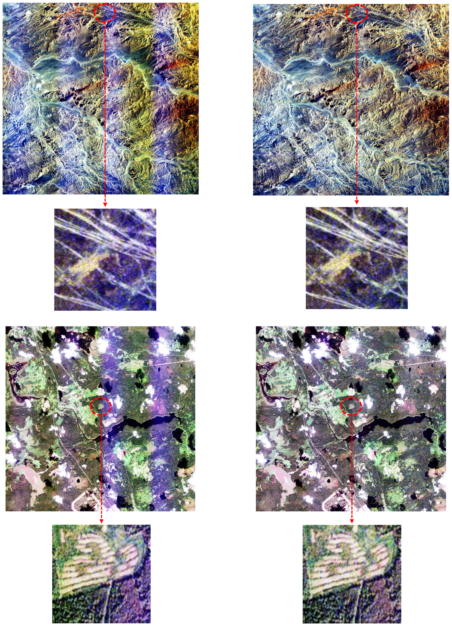
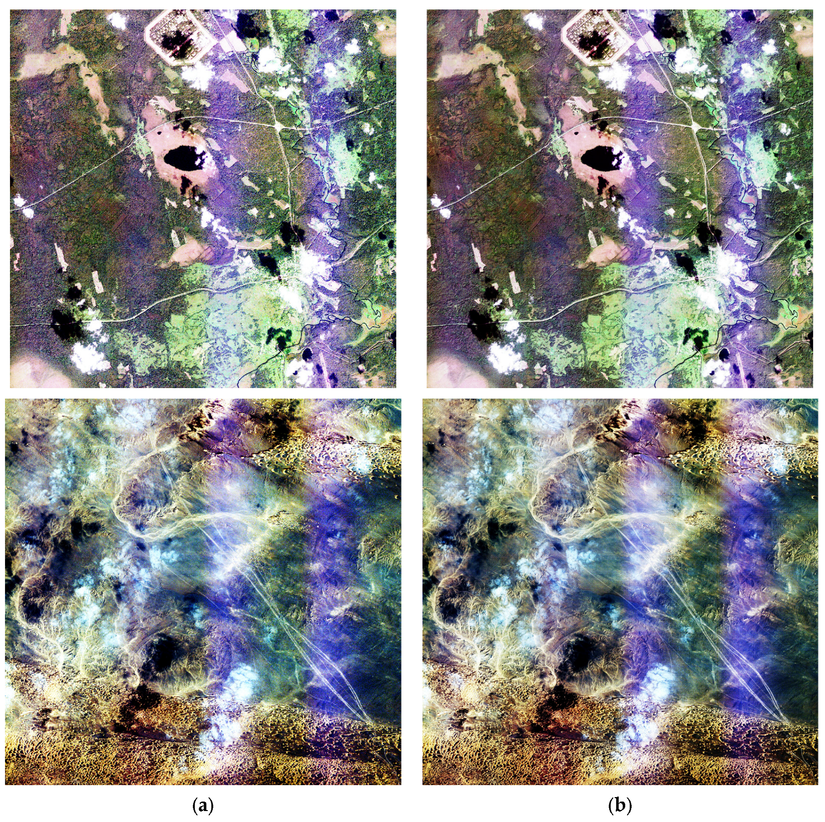
3.4. Experimental Results

After completing the pre-training phase, we evaluated the method’s performance on the validation set of the pre-training dataset. Then, following the fine-tuning phase, we assessed the method’s performance on the validation set of the fine-tuning dataset. Since the color-distorted images in both the pre-training and the fine-tuning datasets have corresponding clean images, we used SSIM and PSNR as evaluation metrics. First, we calculated the differences between the unprocessed (i.e., original, color-distorted) images and the clean images, and then we calculated the difference between the processed images and the clean images. The experimental results are shown in

Table 2. Experimental results on validation sets.

Dataset	Processed	SSIM	PSNR
The validation set of the pre-training dataset	No	0.99983	53.846
	Yes	0.99991	56.383
The validation set of the fine-tuning dataset	No	0.99988	59.213
	Yes	0.99993	62.194

The best results in the table are highlighted in bold.

.

The data in Table 2 demonstrate that the application of the proposed color-distortion correction method leads to improvements in both SSIM and PSNR for the processed images compared to the unprocessed ones. For the validation set of the pre-training dataset, the SSIM increases from 0.99983 for unprocessed images to 0.99991 for processed images, reflecting a small but meaningful improvement of approximately 0.008%. Similarly, the PSNR improves from 53.846 to 56.383, representing a 4.712% increase, which indicates a significant reduction in pixel-level errors and improved image quality. For the validation set of the fine-tuning dataset, the SSIM rises from 0.99988 to 0.99993 after processing, showing a 0.005% improvement. The PSNR sees a more notable increase, from 59.213 to 62.194, marking a 5.034% enhancement. Since the SSIM of the unprocessed images is already very close to 1, the improvement in SSIM after processing is understandably minor, but there is still a measurable enhancement. In both validation sets, the processed images consistently outperform the unprocessed ones; these consistent results across both validation sets underscore the effectiveness of our method, particularly in reducing pixel-level errors and improving image quality while preserving structural similarity.

Additionally, we evaluated the method’s performance on the testing dataset. Since the testing dataset’s real color-distorted images do not have corresponding clean images, we used FCA (Full-Field-of-View Correction Accuracy) as the evaluation metric. FCA was calculated for both the unprocessed images and the processed images, with the results presented in

Table 3. Experimental results on testing dataset.

Metric	Unprocessed Images	Images Processed Using NBNet	Images Processed Using Our Method
FCA	7.9149%	7.9274%	7.7363%

The best result in the table is highlighted in bold.

.

In analyzing the data presented in Table 3, we observe a noticeable improvement in Full-Field-of-View Correction Accuracy (FCA) after applying the proposed color-distortion correction method. Specifically, the FCA decreases from 7.9149% for unprocessed images to 7.7363% for processed images. This reduction of approximately 2.257% suggests that the processed images exhibit improved correction accuracy, further validating the effectiveness of the proposed method. Besides, it is observed that the FCA metric does not improve for images processed using NBNet, indicating that the color distortion in the imagery remains uncorrected. In contrast, images processed using our method show an improvement in the FCA metric, highlighting the progressive advantage of our method.

Figure 14 presents several examples of Jilin-1 KF01 image correction using our method, with the left side showing real color-distorted images and the right side displaying the corrected images. By enlarging the images in Figure 14, it can be observed that image details are well-preserved and the sharpness remains virtually unchanged, indicating that the spatial resolution is effectively maintained.

Figure 15 presents several examples of applying NBNet to correct color distortion in Jilin-1 KF01 series satellite images. The left side shows the real color-distorted images, while the right side displays the corrected results. As seen in Figure 15, the color distortion remains unaddressed after processing with NBNet.

4. Discussion

However, due to the specific color-distortion characteristics of the Jilin-1 KF01 satellite sensors, this study is currently limited to these satellites. The customized nature of our method means it cannot be directly applied to imagery from other types of satellites, as their color-distortion patterns may differ. Nonetheless, the underlying approach presented in this study can serve as a reference for other types of satellites. Specifically, the process involves: (1) analyzing the satellite’s color-distorted imagery and laboratory calibration data to design suitable color-distortion simulation algorithms and construct datasets that reflect the unique color-distortion characteristics of the satellite; (2) selecting an appropriate model and retraining it on the tailored datasets to adapt it for the color-distortion correction task; and (3) employing a post-processing algorithm to remove boundary artifacts caused by block-wise image processing.

5. Conclusions

This paper addresses the issue of color distortion in the Jilin-1 KF01 series satellite imagery by designing a systematic methodology covering color-distortion simulation, model design, and post-processing refinement. First, we conducted an in-depth analysis of the causes of residual color-distortion and designed algorithms to simulate such distortion. Using these simulation algorithms, we created color-distortion datasets containing a large number of paired images (distorted–clean), which served as the foundation for model training. Then, according to the similarities between the principles of a denoising model and the color-distortion correction model, we trained a denoising model from the field of computer vision on color-distortion datasets from scratch, adapting it to effectively handle color-distortion correction in Jilin-1 KF01 imagery. Finally, to address the boundary artifacts commonly encountered during the block-wise processing of single images, we proposed an innovative post-processing algorithm that ensures overall consistency across the image blocks. The experimental results demonstrate that our method can effectively eliminate color distortion in Jilin-1 KF01 series satellite imagery, significantly improving the radiometric quality and practical value of the imagery.

Our method is based on supervised learning and requires a substantial number of paired images (distorted–clean) for training, which are often difficult to obtain directly. To address this challenge, we developed color-distortion simulation algorithms. However, a simulation algorithm cannot simultaneously emulate the diverse color-distortion patterns of different types of satellites, limiting the generalization capability of our method. Therefore, future research could explore the development of unsupervised color-distortion correction algorithms as a promising direction to overcome these limitations.

References

1. Van der Meer, F.D.; Van der Werff, H.M.; Van Ruitenbeek, F.J.; Hecker, C.A.; Bakker, W.H.; Noomen, M.F.; Van Der Meijde, M.; Carranza, E.J.M.; De Smeth, J.B.; Woldai, T. Multi-and hyperspectral geologic remote sensing: A review. Int. J. Appl. Earth Obs. Geoinf. 2012, 14, 112–128. [Google Scholar] [CrossRef]
2. Bevington, A.R.; Menounos, B. Accelerated change in the glaciated environments of western Canada revealed through trend analysis of optical satellite imagery. Remote Sens. Environ. 2022, 270, 112862. [Google Scholar] [CrossRef]
3. Weiss, M.; Jacob, F.; Duveiller, G. Remote sensing for agricultural applications: A meta-review. Remote Sens. Environ. 2020, 236, 111402. [Google Scholar] [CrossRef]
4. Lisboa, F.; Brotas, V.; Santos, F.D. Earth Observation—An Essential Tool towards Effective Aquatic Ecosystems’ Management under a Climate in Change. Remote Sens. 2024, 16, 2597. [Google Scholar] [CrossRef]
5. Hu, R.; Fan, Y.; Zhang, X. Satellite-Derived Shoreline Changes of an Urban Beach and Their Relationship to Coastal Engineering. Remote Sens. 2024, 16, 2469. [Google Scholar] [CrossRef]
6. Wang, Z.; Fan, B.; Yu, D.; Fan, Y.; An, D.; Pan, S. Monitoring the Spatio-Temporal Distribution of Ulva prolifera in the Yellow Sea (2020–2022) Based on Satellite Remote Sensing. Remote Sens. 2022, 15, 157. [Google Scholar] [CrossRef]
7. Pande-Chhetri, R.; Abd-Elrahman, A. De-striping hyperspectral imagery using wavelet transform and adaptive frequency domain filtering. ISPRS J. Photogramm. Remote Sens. 2011, 66, 620–636. [Google Scholar] [CrossRef]
8. Horn, B.K.; Woodham, R.J. Destriping Landsat MSS images by histogram modification. Comput. Graph. Image Process. 1979, 10, 69–83. [Google Scholar] [CrossRef]
9. Kautsky, J.; Nichols, N.K.; Jupp, D.L. Smoothed histogram modification for image processing. Comput. Graph. Image Process. 1984, 26, 271–291. [Google Scholar] [CrossRef]
10. Carfantan, H.; Idier, J. Statistical linear destriping of satellite-based pushbroom-type images. IEEE Trans. Geosci. Remote Sens. 2009, 48, 1860–1871. [Google Scholar] [CrossRef]
11. Rakwatin, P.; Takeuchi, W.; Yasuoka, Y. Stripe noise reduction in MODIS data by combining histogram matching with facet filter. IEEE Trans. Geosci. Remote Sens. 2007, 45, 1844–1856. [Google Scholar] [CrossRef]
12. Gadallah, F.; Csillag, F.; Smith, E. Destriping multisensor imagery with moment matching. Int. J. Remote Sens. 2000, 21, 2505–2511. [Google Scholar] [CrossRef]
13. Kang, Y.; Pan, L.; Sun, M.; Liu, X.; Chen, Q. Destriping high-resolution satellite imagery by improved moment matching. Int. J. Remote Sens. 2017, 38, 6346–6365. [Google Scholar] [CrossRef]
14. Shen, H.; Jiang, W.; Zhang, H.; Zhang, L. A piece-wise approach to removing the nonlinear and irregular stripes in MODIS data. Int. J. Remote Sens. 2014, 35, 44–53. [Google Scholar] [CrossRef]
15. Sun, L.; Neville, R.; Staenz, K.; White, H.P. Automatic destriping of Hyperion imagery based on spectral moment matching. Can. J. Remote Sens. 2008, 34, S68–S81. [Google Scholar] [CrossRef]
16. Chen, J.; Shao, Y.; Guo, H.; Wang, W.; Zhu, B. Destriping CMODIS data by power filtering. IEEE Trans. Geosci. Remote Sens. 2003, 41, 2119–2124. [Google Scholar] [CrossRef]
17. Simpson, J.J.; Gobat, J.I.; Frouin, R. Improved destriping of GOES images using finite impulse response filters. Remote Sens. Environ. 1995, 52, 15–35. [Google Scholar] [CrossRef]
18. Chen, J.; Lin, H.; Shao, Y.; Yang, L. Oblique striping removal in remote sensing imagery based on wavelet transform. Int. J. Remote Sens. 2006, 27, 1717–1723. [Google Scholar] [CrossRef]
19. Torres, J.; Infante, S.O. Wavelet analysis for the elimination of striping noise in satellite images. Opt. Eng. 2001, 40, 1309–1314. [Google Scholar]
20. Ranchin, T.; Wald, L. The wavelet transform for the analysis of remotely sensed images. Int. J. Remote Sens. 1993, 14, 615–619. [Google Scholar] [CrossRef]
21. Shen, H.; Zhang, L. A MAP-based algorithm for destriping and inpainting of remotely sensed images. IEEE Trans. Geosci. Remote Sens. 2008, 47, 1492–1502. [Google Scholar] [CrossRef]
22. Bouali, M.; Ladjal, S. Toward optimal destriping of MODIS data using a unidirectional variational model. IEEE Trans. Geosci. Remote Sens. 2011, 49, 2924–2935. [Google Scholar] [CrossRef]
23. Liu, X.; Lu, X.; Shen, H.; Yuan, Q.; Jiao, Y.; Zhang, L. Stripe noise separation and removal in remote sensing images by consideration of the global sparsity and local variational properties. IEEE Trans. Geosci. Remote Sens. 2016, 54, 3049–3060. [Google Scholar] [CrossRef]
24. Lu, X.; Wang, Y.; Yuan, Y. Graph-regularized low-rank representation for destriping of hyperspectral images. IEEE Trans. Geosci. Remote Sens. 2013, 51, 4009–4018. [Google Scholar] [CrossRef]
25. Wang, M.; Zheng, X.; Pan, J.; Wang, B. Unidirectional total variation destriping using difference curvature in MODIS emissive bands. Infrared Phys. Techn. 2016, 75, 1–11. [Google Scholar] [CrossRef]
26. Zhou, G.; Fang, H.; Yan, L.; Zhang, T.; Hu, J. Removal of stripe noise with spatially adaptive unidirectional total variation. Optik 2014, 125, 2756–2762. [Google Scholar] [CrossRef]
27. He, W.; Zhang, H.; Zhang, L.; Shen, H. Total-variation-regularized low-rank matrix factorization for hyperspectral image restoration. IEEE Trans. Geosci. Remote Sens. 2015, 54, 178–188. [Google Scholar] [CrossRef]
28. He, W.; Zhang, H.; Shen, H.; Zhang, L. Hyperspectral image denoising using local low-rank matrix recovery and global spatial–spectral total variation. IEEE J. Sel. Top. Appl. Earth Obs. Remote Sens. 2018, 11, 713–729. [Google Scholar] [CrossRef]
29. Zhang, H.; He, W.; Zhang, L.; Shen, H.; Yuan, Q. Hyperspectral image restoration using low-rank matrix recovery. IEEE Trans. Geosci. Remote Sens. 2013, 52, 4729–4743. [Google Scholar] [CrossRef]
30. Xie, W.; Li, Y. Hyperspectral imagery denoising by deep learning with trainable nonlinearity function. IEEE Geosci. Remote Sens. Lett. 2017, 14, 1963–1967. [Google Scholar] [CrossRef]
31. Wang, Z.; Ng, M.K.; Zhuang, L.; Gao, L.; Zhang, B. Nonlocal self-similarity-based hyperspectral remote sensing image denoising with 3-D convolutional neural network. IEEE Trans. Geosci. Remote Sens. 2022, 60, 1–17. [Google Scholar] [CrossRef]
32. Han, L.; Zhao, Y.; Lv, H.; Zhang, Y.; Liu, H.; Bi, G. Remote sensing image denoising based on deep and shallow feature fusion and attention mechanism. Remote Sens. 2022, 14, 1243. [Google Scholar] [CrossRef]
33. Huang, Z.; Zhu, Z.; Wang, Z.; Shi, Y.; Fang, H.; Zhang, Y. DGDNet: Deep gradient descent network for remotely sensed image denoising. IEEE Geosci. Remote Sens. Lett. 2023, 20, 1–5. [Google Scholar] [CrossRef]
34. Xu, Y.; Luo, W.; Hu, A.; Xie, Z.; Xie, X.; Tao, L. TE-SAGAN: An improved generative adversarial network for remote sensing super-resolution images. Remote Sens. 2022, 14, 2425. [Google Scholar] [CrossRef]
35. Wang, P.; Bayram, B.; Sertel, E. A comprehensive review on deep learning based remote sensing image super-resolution methods. Earth Sci. Rev. 2022, 232, 104110. [Google Scholar] [CrossRef]
36. Dong, X.; Sun, X.; Jia, X.; Xi, Z.; Gao, L.; Zhang, B. Remote sensing image super-resolution using novel dense-sampling networks. IEEE Trans. Geosci. Remote Sens. 2020, 59, 1618–1633. [Google Scholar] [CrossRef]
37. Zhang, S.; Yuan, Q.; Li, J.; Sun, J.; Zhang, X. Scene-adaptive remote sensing image super-resolution using a multiscale attention network. IEEE Trans. Geosci. Remote Sens. 2020, 58, 4764–4779. [Google Scholar] [CrossRef]
38. Chang, Y.; Yan, L.; Fang, H.; Zhong, S.; Liao, W. HSI-DeNet: Hyperspectral image restoration via convolutional neural network. IEEE Trans. Geosci. Remote Sens. 2018, 57, 667–682. [Google Scholar] [CrossRef]
39. Zhong, Y.; Li, W.; Wang, X.; Jin, S.; Zhang, L. Satellite-ground integrated destriping network: A new perspective for EO-1 Hyperion and Chinese hyperspectral satellite datasets. Remote Sens. Environ. 2020, 237, 111416. [Google Scholar] [CrossRef]
40. Wang, C.; Xu, M.; Jiang, Y.; Zhang, G.; Cui, H.; Li, L.; Li, D. Translution-SNet: A semisupervised hyperspectral image stripe noise removal based on transformer and CNN. IEEE Trans. Geosci. Remote Sens. 2022, 60, 1–14. [Google Scholar] [CrossRef]
41. Wang, C.; Xu, M.; Jiang, Y.; Deng, G.; Lu, Z.; Zhang, G.; Cui, H. Hyperspectral image stripe removal network with cross-frequency feature interaction. IEEE Trans. Geosci. Remote Sens. 2021, 60, 1–15. [Google Scholar] [CrossRef]
42. Wang, C.; Xu, M.; Jiang, Y.; Zhang, G.; Cui, H.; Deng, G.; Lu, Z. Toward real hyperspectral image stripe removal via direction constraint hierarchical feature cascade networks. Remote Sens. 2022, 14, 467. [Google Scholar] [CrossRef]
43. Wang, Z.; Wang, G.; Pan, Z.; Zhang, J.; Zhai, G. Fast stripe noise removal from hyperspectral image via multi-scale dilated unidirectional convolution. Multimed. Tools Appl. 2020, 79, 23007–23022. [Google Scholar] [CrossRef]
44. Guo, Q.; Zhang, C.; Zhang, Y.; Liu, H. An efficient SVD-based method for image denoising. IEEE Trans. Circuits Syst. Video Technol. 2015, 26, 868–880. [Google Scholar] [CrossRef]
45. Aharon, M.; Elad, M.; Bruckstein, A. K-SVD: An algorithm for designing overcomplete dictionaries for sparse representation. IEEE Trans. Signal Process. 2006, 54, 4311–4322. [Google Scholar] [CrossRef]
46. Cheng, S.; Wang, Y.; Huang, H.; Liu, D.; Fan, H.; Liu, S. Nbnet: Noise basis learning for image denoising with subspace projection. In Proceedings of the IEEE/CVF Conference on Computer Vision and Pattern Recognition, Nashville, TN, USA, 20–25 June 2021; pp. 4896–4906. [Google Scholar]
47. Wang, Z.; Bovik, A.C.; Sheikh, H.R.; Simoncelli, E.P. Image quality assessment: From error visibility to structural similarity. IEEE Trans. Image Process. 2004, 13, 600–612. [Google Scholar] [CrossRef]
48. Hore, A.; Ziou, D. Image quality metrics: PSNR vs. SSIM. In Proceedings of the 2010 20th International Conference on Pattern Recognition, Istanbul, Turkey, 23–26 August 2010; pp. 2366–2369. [Google Scholar]
49. Li, L.; Jiang, Y.; Shen, X.; Li, D. Long-term assessment and analysis of the radiometric quality of standard data products for Chinese Gaofen-1/2/6/7 optical remote sensing satellites. Remote Sens. Environ. 2024, 308, 114169. [Google Scholar] [CrossRef]
Figure 1. Jilin-1 KF01 image comparison: (a) Image before histogram matching; (b) Image after histogram matching.
Remotesensing 16 04721 g001
Figure 2. Jilin-1 KF01 laboratory calibration images: (a) Original calibration image; (b) Corrected calibration image; (c) Column-wise mean; (d) Column-wise standard deviation.
Remotesensing 16 04721 g002
Figure 3. Comparison of color-distortion patterns: (a) Sea images; (b) Color-distortion patterns.
Remotesensing 16 04721 g003
Figure 4. Analysis of Jilin-1 KF01 laboratory calibration images: (a) Original calibration images; (b) Column-wise mean.
Remotesensing 16 04721 g004
Figure 5. Analysis of satellite-transmitted remote sensing image: (a) Sea image; (b) Column-wise mean of Band 1; (c) Column-wise mean of Band 2; (d) Column-wise mean of Band 3.
Remotesensing 16 04721 g005
Figure 6. Simulated color-distortion pattern in the pre-training dataset.
Remotesensing 16 04721 g006
Figure 7. Simulated color-distortion pattern in the fine-tuning dataset.
Remotesensing 16 04721 g007
Figure 8. Process of correcting color-distorted image block.
Remotesensing 16 04721 g008
Figure 9. Schematic diagram of the overlapping regions of color-distortion pattern blocks in the horizontal direction.
Remotesensing 16 04721 g009
Figure 10. Post-processing: (a) Real color-distorted Jilin-1 KF01 image; (b) Overlap 0 pixels; (c) Overlap 140 pixels; (d) After horizontal post-processing; (e) After vertical post-processing; (f) Corrected image.
Remotesensing 16 04721 g010
Figure 11. An example from the pre-training dataset: (a) Clean image; (b) Color-distorted image; (c) Simulated color-distortion pattern in Band 1; (d) Simulated color-distortion pattern in Band 2; (e) Simulated color-distortion pattern in Band 3.
Remotesensing 16 04721 g011
Figure 12. An example from the fine-tuning dataset: (a) Clean image; (b) Color-distorted image; (c) Simulated color-distortion pattern in Band 1; (d) Simulated color-distortion pattern in Band 2; (e) Simulated color-distortion pattern in Band 3.
Remotesensing 16 04721 g012
Figure 13. An example from the testing dataset: (a) Real color-distorted image; (b) Column-wise mean of Band 1 after subtracting its overall mean; (c) Column-wise mean of Band 2 after subtracting its overall mean; (d) Column-wise mean of Band 3 after subtracting its overall mean.
Remotesensing 16 04721 g013
Figure 14. Correction results for our method: (a) Real color-distorted Jilin-1 KF01 images; (b) Corrected images.
Remotesensing 16 04721 g014aRemotesensing 16 04721 g014b
Figure 15. Correction results for NBNet: (a) Real color-distorted Jilin-1 KF01 images; (b) Corrected images.
Remotesensing 16 04721 g015