Monitoring Saltmarsh Restoration in the Upper Bay of Fundy Using Multi-Temporal Sentinel-2 Imagery and Random Forests Classifier

Abstract

Saltmarshes provide important ecosystem services, including coastline protection, but face decline due to human activities and climate change. There are increasing efforts to conserve and restore saltmarshes worldwide. Our study evaluated the effectiveness of Sentinel-2 satellite imagery to monitor landcover changes using a saltmarsh restoration project undergoing its 9th to 12th year of recovery in the megatidal Bay of Fundy in Maritime Canada. Specifically, in 2019–2022, five satellite images per growing season were acquired. Random Forests classification for 13 landcover classes (ranging from bare mud to various plant communities) achieved a high overall classification accuracy, peaking at 96.43% in 2021. Field validation points confirmed this, with high validation accuracies reaching 93.02%. The classification results successfully distinguished ecologically significant classes, such as Spartina alterniflora–S. patens mix. Our results reveal the appearance of high marsh species in restoration sites and elevational-based zonation patterns, indicating progression. They demonstrate the potential of Sentinel-2 imagery for monitoring saltmarsh restoration projects in north temperate latitudes, aiding management efforts.

1. Introduction

Saltmarshes are intertidal wetlands comprising salt-tolerant vegetation [1,2]. This vegetation includes grasses and sedges that help trap sediment, contributing to marsh development and shoreline stabilization [3,4,5]. Elevational changes within the marsh influence the distribution of plant communities according to the degree of tidal inundation, salinity tolerance, and competitive ability of individual plant species [6,7,8,9]. Saltmarshes can experience high rates of sediment deposition [10,11] and a relatively slow rate of plant matter decomposition [3,12], allowing the storage of large amounts of carbon over time [13,14]. These coastal ecosystems support an abundant faunal community, including invertebrates [11,15], fish [16], and birds [17].

Saltmarsh areas have declined globally due to anthropogenic impacts and climate change [18,19,20]. For example, the Bay of Fundy in Maritime Canada is estimated to have an 85% loss in its natural saltmarshes after their conversion to mainly agricultural land with the settlement of European and American colonists since the 17th century [21,22,23]. Even today, in Maritime Canada and other regions of the world, the combined effect of sea level rise (globally, and locally due to ongoing subsidence of the crust; [24]) and the anthropogenic conversion of coastlines for other uses has led to coastal squeeze, which is the prevention of the natural landward advancement of saltmarshes [25,26]. The United Nations General Assembly declared that 2021–2030 is the “UN Decade on Ecosystem Restoration”, hence emphasizing the need for major restoration programs [27]. Given the global loss of and acknowledged ecosystem services provided by saltmarshes, there is an increasing effort to conserve and restore saltmarshes [20,28]. The conservation and restoration of saltmarshes require the effective monitoring and mapping of saltmarsh vegetation to allow a better understanding of marsh dynamics associated with accretion and erosion patterns, and management projects. Satellite imagery bypasses the challenge brought by often remote and difficult terrain such as saltmarshes and can be suitable for monitoring on a relatively large spatial scale. Saltmarsh vegetation mapping has been conducted using various satellite-based sensors and classifiers (Table 1). Several studies in Table 1 used Sentinel-2 images because these images have a relatively high number of bands, including the red, red-edge, and near-infrared bands, which are well-suited for vegetation detection and mapping. Sentinel-2 images have a high temporal resolution (between 2 and 6 days), due to two available satellites (2A and 2B), and a high spatial resolution (10 m), making them suitable for detailed landcover mapping.

The first goal of our study was to evaluate the use of Sentinel-2 imagery to map vegetation in new (restoration) and established (reference) saltmarshes located in Aulac, New Brunswick, Canada. The second goal was to determine changes in vegetation patterns in the marshes, particularly in the saltmarshes undergoing restoration. We used a total of 20 images acquired between 2019 and 2022, with 5 images per year across different seasons, to compare the temporal and spatial vegetation patterns in both the restoration and the reference sites. Using multi-temporal images is expected to produce better accuracies than using a single image from individual months, as already shown in [29]. In our study, we used a non-parametric supervised classifier Random Forests (RF), an algorithm originally developed by [30], that has been shown to outperform other supervised classifiers for vegetation mapping [31,32,33,34,35,36,37]. It also provides the relative importance of input features (i.e., band reflectance and vegetation index images in our study) in the classification [31]. The resulting classified images were validated with field-based data. To our knowledge, our study is the first to use Sentinel-2 images for the vegetation mapping of saltmarshes in the Bay of Fundy, which experiences relatively special conditions because of its macro-tidal regime and cold winters [38,39]. We also considered a higher number of landcover classes (13) compared to other similar studies that only had up to 10 classes (Table 1). Such a high number of classes enabled us to monitor ecologically significant plant communities occurring in specific zones of the marshes. We were even able to map the landcover at the species level despite the 10 m spatial resolution of the imagery. Our developed methodology should enable future studies to monitor saltmarsh vegetation progression in north temperate latitudes using Sentinel-2 imagery.

Table 1. Comparison of the classification accuracy obtained by previous studies using satellite imagery for saltmarsh vegetation mapping based on the sensor and the classifier.

Sensor	Classifier *	Classification Accuracy (%)	Number of Classes	Season	Region	Reference
Sentinel-2	OBIA + RF	99	4	Summer	Turkey	[40]
	RF	91	5	All seasons	China	[41]
	Supervised hierarchical classifier	80	8	Spring, Summer, Fall	Italy	[42]
Sentinel-1 and Sentinel-2	RF	92	3	Summer	China	[43]
Sentinel-2 and Worldview-2,3	OBIA + RF	93	10	Spring	USA	[44]
	SVM	93	8	Summer, Fall	Ontario, Canada	[45]
	MLC	75	8	Summer, Fall	Ontario, Canada	[45]
SPOT and IRS	MLC	68	6	Spring, Summer	UK	[46]
AVNIR-2 and Alos PalSAR	OBIA + RF	82	9	Spring	China	[47]
Alos PalSAR	OBIA + RF	89	7	Fall	China	[48]
Sentinel-1	RF	87	5	Multiple	China	[49]
GF-1, ZY-3	OBIA + RF	84	6	Multiple	China	[50]

(*) RF = Random Forests, MLC = Maximum Likelihood Classification, OBIA = Object-based Image Analysis, SVM = Support Vector Machine.

Table 1. Comparison of the classification accuracy obtained by previous studies using satellite imagery for saltmarsh vegetation mapping based on the sensor and the classifier.

Sensor	Classifier *	Classification Accuracy (%)	Number of Classes	Season	Region	Reference
Sentinel-2	OBIA + RF	99	4	Summer	Turkey	[40]
	RF	91	5	All seasons	China	[41]
	Supervised hierarchical classifier	80	8	Spring, Summer, Fall	Italy	[42]
Sentinel-1 and Sentinel-2	RF	92	3	Summer	China	[43]
Sentinel-2 and Worldview-2,3	OBIA + RF	93	10	Spring	USA	[44]
	SVM	93	8	Summer, Fall	Ontario, Canada	[45]
	MLC	75	8	Summer, Fall	Ontario, Canada	[45]
SPOT and IRS	MLC	68	6	Spring, Summer	UK	[46]
AVNIR-2 and Alos PalSAR	OBIA + RF	82	9	Spring	China	[47]
Alos PalSAR	OBIA + RF	89	7	Fall	China	[48]
Sentinel-1	RF	87	5	Multiple	China	[49]
GF-1, ZY-3	OBIA + RF	84	6	Multiple	China	[50]

(*) RF = Random Forests, MLC = Maximum Likelihood Classification, OBIA = Object-based Image Analysis, SVM = Support Vector Machine.

2. Materials and Methods

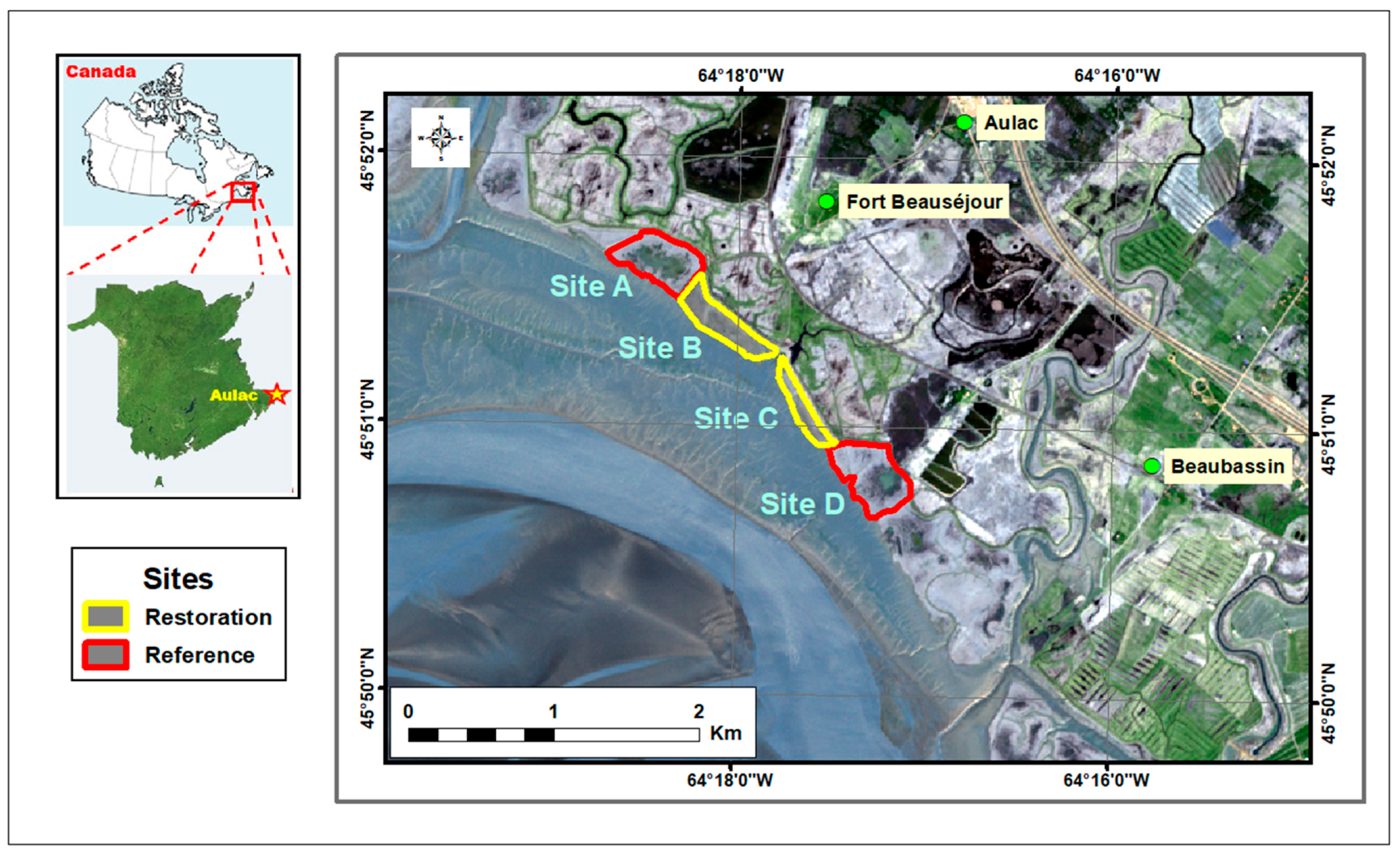
2.1. Study Area

The Aulac saltmarsh complex (45°51′16″ N, 64°17′50″ W) is located at the head of Cumberland Basin in the upper Bay of Fundy, near Fort Beauséjour (Figure 1). The saltmarsh restoration project started in 2010 and was the first managed realignment project in Maritime Canada [11,39]. In October 2010, the old agricultural dike was mechanically breached to reintroduce tidal seawater and initiate the restoration process in former pastureland sites (sites B and C). At that time, these sites to be restored were at a much lower elevation compared to the reference saltmarsh sites (sites A and D) [11,51]. Since the dike breaching, the recovery rate of the pioneer marsh species, i.e., saltwater cordgrass (Spartina alterniflora L.; syn. Sporobolus alterniflorus [52,53]), was monitored along with the rest of the plant community in the restoration sites B and C [11,54]. The colonization and spread dynamics leading to a low marsh zone plant community were compared to the two reference sites (established saltmarshes, sites A and D), which have a predominantly high marsh zone plant community. Species in the latter community include the dominant saltmarsh hay (Spartina patens (Aiton) Muhl; syn. Sporobolus pumilus), along with seaside arrowgrass (Triglochin maritima L.), sea plantain (Plantago maritima L.), and black rush (Juncus gerardii L.), and near the terrestrial border, saltmarsh bulrush (Bolboschoenus maritimus (L.) Palla) and scaly sedge (Carex paleacea Schreb. ex Wahlenb.).

2.2. Sentinel-2 Images

Sentinel-2 imagery (Level 2A, and Level 2B) was acquired by two satellites, Sentinel-2A and Sentinel-2B, respectively, operated by the European Space Agency (Supplementary Table S1). Both satellites are in 180° orbit within each other and provide images over a revisit time of 5 days at the Equator [55]. Sentinel-2 satellites have a Multi-Spectral Imagery (MSI) sensor with usable twelve bands. Seven of the twelve bands are in the infrared region of the electromagnetic spectrum (

Table 2. Characteristics of the spectral bands from the Sentinel-2 satellite.

Band	Band Name	Wavelength (nm)		Spatial Resolution (m)
		Sentinel-2A	Sentinel-2b
B1	Coastal	433–453	442–452	60
B2	Blue	460–525	460–525	10
B3	Green	542–577	526–591	10
B4	Red	650–680	649–680	10
B5	Red-Edge 1	697–711	696–711	20
B6	Red-Edge 2	734–748	733–746	20
B7	Red-Edge 3	773–792	770–789	20
B8	NIR	780–885	781–885	10
B8a	Narrow NIR (NIRn)	854–875	854–875	20
B9	Water Vapor	926–964	923–963	60
B11	SWIR1	1569–1659	1563–1657	20
B12	SWIR2	2115–2289	2094–2278	20

). The Sentinel-2 MSI sensor has the advantage of having all the bands needed to map vegetation, including the red band that is strongly absorbed by chlorophyl and the near-infrared band that is strongly reflected by vegetation. In addition, it has three bands in the red-edge region that were already shown to be essential for vegetation mapping and monitoring [56,57]. [56] also showed that the red-edge bands and their derived vegetation indices improve cover mapping. For practical reasons and to simplify the image processing as much as possible, we did not proceed to the band adjustment between the Sentinel-2A and Sentinel-2B images. Such band adjustment is necessary to compare spectral signatures produced by different sensors, such as the Landsat 8-9 OLI and the Sentinel-2 MSI [58]. By contrast, the difference in wavelength range between the Sentinel-2A and Sentinel-2B spectral bands is small (less than 21 nm for the lower wavelength limit for Band 12) and can be considered negligible for our study which is about mapping plant communities. The image spatial resolution ranges from 10 m to 60 m depending on the band (Table 2). All acquired images have an angle of view relative to the nadir of 20.6°, a swath width from the nadir of 290 km, and a radiometric resolution of 12 bits/pixel.

To analyze temporal changes over the growing season, we selected five images from five consecutive months spanning from May to September, for each year from 2020 to 2022. Based on availability, images for the year 2019 were dated from June to October. The images were acquired for cloud-free atmospheric conditions (manually verified for our study area) so that landscape features within the saltmarshes could be fully visible. We acquired images preferably at or near low tide to allow for the lower elevational areas of the marsh to be visible on the imagery (although this could not always be achieved; see below). The environmental conditions at the time of image acquisition included sun position, air temperature and relative humidity measured near ground level, tidal height, and the amount of precipitation in the previous 10 days (Supplementary Table S2). Since there was no presence of cloud in the images over the area of interest (AOI), there was no need to record the percent cloud cover for each image. Sun zenith and azimuth angles were recorded from the Earth System Research Laboratory of the National Oceanic and Atmospheric Administration (NOAA). The sun’s zenith was high enough to ensure a minimal error due to shadows cast on the spectral response. Air temperature, relative humidity, and precipitation amount were obtained from Environment and Climate Change Canada at the Nappan AAFC weather station, Nova Scotia, which is 11 km from the study area. Tidal height (m above Chart Datum) was obtained for Pecks Point tidal station of the Canadian Hydrographic Service from Fisheries and Oceans Canada. All these data allowed us to better understand ground conditions, such as soil humidity and the state of the salt pools (i.e., depressions in the marsh platform that retain water at low tide), in the reference and restoration sites to later aid in photointerpretation and image classification. Tidal height informed us of whether marsh vegetation was submerged by tidal water at the time of image acquisition. Submergence occurred for the restoration sites and the narrow low marsh zone in the reference sites on four satellite image acquisition dates when the tide was greater than 12 m (Supplementary Table S2). The reference sites A and D (with the marsh platform at approximately 6.88 m CGVD28) have a higher elevation than the restoration sites B and C, with the marsh platform at approximately 5.95 m (CGVD28 data for 2021 from J. Ollerhead, Mount Allison University). These reference sites have low-elevation areas near and in the creeks, which are at similar elevations as those of the restoration sites.

2.3. Ground Truth Data

For 2019–2021, a total of 301 validation pixels per year, measuring 10 m by 10 m, were used. For 2022, only 224 validation pixels were used because many 2019–2021 validation pixels were located inside new transitional zones in the reference sites. Each geolocated validation pixel is located inside a field square having a minimum of 15 m by 15 m in size, which is larger than the resampled image resolution of 10 m (Table 2) to avoid edge features being included in the reflectance measurement for each pixel. The identification of validation pixel is based on a 0.5 cm by 0.5 cm quadrat established to determine the species composition from ground pictures as described in [54,59]. The field measurements were collected monthly between June and August to consider the seasonal variation in the vegetation. These plots were strategically placed to represent dominant landcover classes. Within the validation plots, photographs were taken using a field camera to record the ground-level observations and species composition.

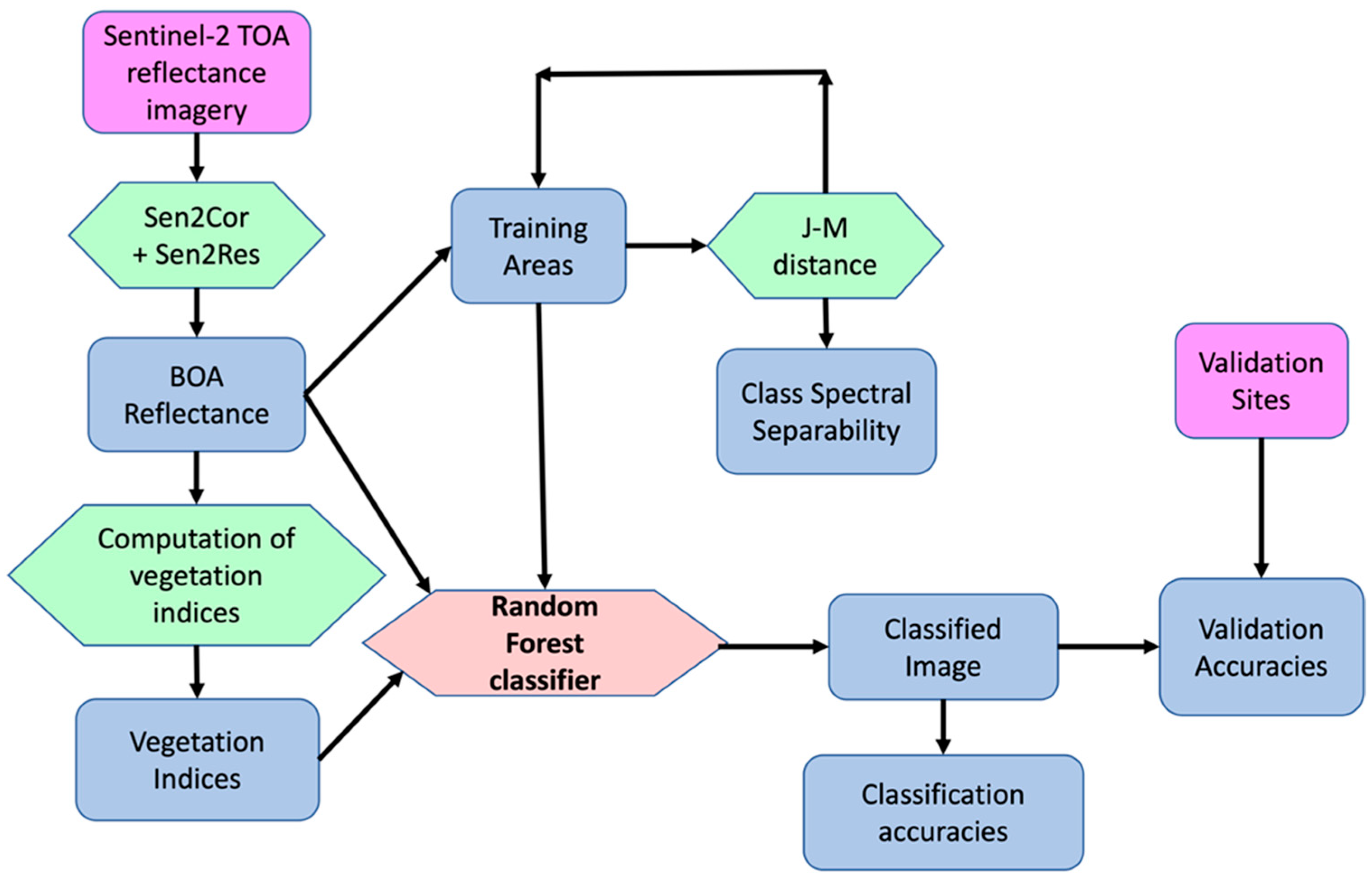
2.4. Image Processing

Our methodology for each year’s set of 5 images included the pre-classification processing of Sentinel-2 images, computation of vegetation indices, delineation of training areas, supervised classification, and validation of the classified images (Figure 2).

Given that some spectral bands have a different spatial resolution (Table 2), the Sen2Res algorithm of SNAP [60,61] was used to resample all the band images to a 10 m resolution. Based on the algorithm of Pignatale [62], the Sen2Cor processor of SNAP was used to apply atmospheric corrections to the images to eliminate aerosol scattering, sun glint, and other atmospheric effects. The resulting images are bottom of atmosphere (BoA) reflectance bands with a resolution of 10 m. These images were then imported into the PCI^® Catalyst 2022 image processing software (PCI Geomatics Group Inc., Richmond Hill, ON, Canada) to mask them to include only the two restoration sites and two reference sites (Figure 1). The BoA reflectance images were then used to compute vegetation indices (

Table 3. Vegetation indices used in the study.

Index	Index Name	Formula	Reference
DVI	Difference vegetation index	NIR - R	[66]
GDVI	Green difference vegetation index	NIR - G	[63]
GNDVI	Green normalized difference vegetation index	(NIR - G) / (NIR + G)	[67]
GRVI	Green ratio vegetation index	NIR / G	[63]
NDAVI	Normalized difference aquatic vegetation index	(NIR - B) / (NIR + B)	[68]
NDVI	Normalized difference vegetation index	(NIR - R) / (NIR + R)	[69]
NDRE	Normalized difference red-edge vegetation index	(NIR - RE) / NIR + RE)	[70]
NG	Normalized green vegetation index	G / (NIR + R + G)	[63]
NNIR	Normalized near-infrared vegetation index	NIR / (NIR + R + G)	[63]
NR	Normalized red vegetation index	R / (NIR + R + G)	[63]
RVI	Red ratio vegetation index	NIR / R	[64]
REVI	Red-edge simple ratio vegetation index	NIR / RE	[70]
WAVI	Water-adjusted vegetation index	1.5 × (NIR - B) / (NIR + B + 0.5)	[68]

). The 13 indices were chosen because they have been shown to detect different vegetation types well [63,64,65].

2.5. Image Classification

For a given year, all the monthly reflectance bands (12) and vegetation indices (13) were combined into a single raster image file, using the PCI^® Catalyst image processing software. This image processing provided a total of 125 features (5 months × 25 features/month) that were inputted into the Random Forests (RF) classifier, a non-parametric decision tree-type supervised classification algorithm. Originally designed for use by the machine learning community, this algorithm is becoming increasingly popular for remote sensing applications, showing numerous advantages when compared to other classical classification methods [36]. Developed from the work of Breiman et al. [30,71], RF does not assume a normal distribution of the input data [30]. In addition, RF is not sensitive to noise or overclassifying and provides an estimate of the importance of each input image for the classification [32,33]. The specific RF algorithm used for our study was developed in the R programming language (version 4.1.0), with a script originally written by Horning [72] that uses the maptools, sp, randomForest, raster, and rgal packages.

The RF classifier works by generating a series of decision trees, which are predictive models that use a set of binary rules to calculate a target value. This classifier was calibrated using two thirds of the training area data, which are called “In Bag” data, creating independent decision trees that were subsequently combined into the final classification map [33]. In our study, “In Bag” data were selected to create 500 independent decision trees, in which each tree used a randomized subset of the input data with slightly different categories. The remaining third of the training area data, the “Out of Bag” (OOB), was used to test the forest to validate the resulting classification.

The RF classifier was also set with the default number of variables randomly sampled as candidates at the split of every node (i.e., mtry). The default value for mtry for a classification is calculated as the square root of the number of predicator variables randomly sampled as candidates at each split of every node. Using the default value provides a setting that includes all pixels that will be randomly sampled as candidates at each split of every node. The RF algorithm can be run in two versions: “all-polygon” and “sub-polygon”. The all-polygon version uses all the pixels within the training area polygons, while the sub-polygon version randomly selects a user-determined number of training pixels for each class. In our study, the all-polygon setting was used, as it has the advantage of taking account of the actual class size and providing a better image classification.

Another advantage of using RF is that the algorithm outputs a variable importance plot. This plot ranks the importance of each variable to the classification, indicating how much an individual variable input was used by the RF classifier to make its prediction. Indeed, the higher the mean decrease in accuracy related to a specific band, the more useful a given band is for performing the classification [73,74].

The supervised classification with RF requires delineating training areas for each landcover class (

Table 4. Landcover classes and their associated description for the study.

Class Number	Name	Description
1	Bare mud	Areas with no vegetation to minimal vegetation (<5%), covered in mud, such as the tidal flats.
2	Water	Wet areas visible throughout the year in salt pools (specifically in the reference marshes).
3	Sparse S. alterniflora	Monoculture of saltwater cordgrass Spartina alterniflora occurring in the restoration sites, with sparse foliage and visible ground mud on imagery.
4	Dense S. alterniflora	Monoculture of S. alterniflora occurring in the restoration sites, with denser foliage with no vegetation to minimal mud visibility on imagery.
5	S. patens dominant	Community of saltmarsh vegetation dominated by saltmarsh hay Spartina patens that typically grow at higher elevation. Other species include sea lavender (Limonium carolinianum), sea plantain (Plantago maritima), orach (Atriplex spp.), and seaside goldenrod (Solidago sempervirens).
6	S. patens−J. gerardii mix	A mix of S. patens and black rush Juncus gerardii at about a 50/50 ratio.
7	S. alterniflora−S. patens mix	A mix of S. alterniflora and S. patens occurring at about a 50/50 ratio.
8	J. gerardii−C. paleacea mix	A mix of J. gerardii and scaly sedge Carex paleacea occurring at about a 50/50 ratio.
9	C. paleacea− S. pectinata mix	A mix of C. paleacea and freshwater cordgrass Spartina pectinata occurring at about a 50/50 ratio.
10	Terrestrial vegetation on dike	Saline-intolerant terrestrial vegetation growing over and along the dike.
11	Dike	Non-vegetated path made of soil and gravel that separates the farmland from the saltmarshes.
12	Vegetated water	Water from salt pools of the reference sites that have algae and other sub-surface aquatic vegetation.
13	S. alterniflora  dominant	Areas in the reference sites that are high in moisture content due to proximity to salt pools, creeks, and similar depressions where S. alterniflora grows.

). The delineation of training areas of usually 400 m² (corresponding to 4 pixels, i.e., squares of 2 pixels by 2 pixels) was performed by the photointerpretation of false color composites that enhanced specific landscape features. The location of these training areas is confirmed by photos taken at ground level (Supplementary Table S3). For instance, the red, NIR, and green band reflectance images from July were most useful for examining live vegetation because the vegetation was fully developed and had not started senescing yet. The placements of training areas were conducted based on the consistent presence of the features of interest throughout the months. Some classes (e.g., Class 2, Water) posed a challenge due to varying periods of dryness or inundation throughout the time series. To overcome this challenge, training pixels were placed individually instead of using a cluster of four pixels. This allowed us to select the deepest parts of the salt pools that would consistently show the presence of water despite the dry periods.

Amongst the 13 classes used in the classification of all sites (Table 4), there are 4 non-vegetated classes (Classes 1, 2, 11, 12). Class 12 (Vegetated water) primarily consists of algal cover, including submerged and sub-surface aquatic vegetation, which are not typical halotolerant. Therefore, in our study, this class is categorized as unvegetated. Amongst the nine remaining vegetated classes, two are restoration site-focused classes (Classes 3, 4), and six are reference site-focused classes (Classes 5–9, 13). Note that S. alterniflora dominant (Class 13) is found in the low marsh zone and lower depression areas of the reference sites and should not be confused with Classes 3 and 4, which are present in the restoration sites. Class 13 (S. alterniflora dominant) shows different spectral signatures compared to the restoration Classes 3 and 4 likely due to the different growing conditions present in the reference sites and, therefore, is considered separate in the analysis. Terrestrial vegetation on the dike (Class 10) was recorded to understand the state of the dike over the years.

Training areas (

Table 5. Number of training areas and validation points according to the year and landcover class in the study.

Class Number	Landcover Classes	Training				Validation
		2019	2020	2021	2022	2019	2020	2021	2022
1	Bare mud	94	48	85	81	37	35	34	18
2	Water	22	26	28	22	21	19	15	7
3	Sparse S. alterniflora	49	46	63	36	19	25	24	26
4	Dense S. alterniflora	47	49	54	53	19	15	30	18
5	S. patens dominant	65	67	67	68	35	29	48	28
6	S. patens−J. gerardii mix	23	18	28	23	12	22	16	21
7	S. alterniflora−S. patens mix	42	32	45	45	13	22	30	29
8	J. gerardii−C. paleacea mix	37	33	33	36	18	9	14	12
9	C. paleacea−S. pectinata mix	16	27	26	25	10	17	14	15
10	Terrestrial vegetation on dike	59	45	39	45	33	22	15	11
11	Dike	67	54	55	55	24	30	24	13
12	Vegetated water	45	46	36	48	21	24	20	15
13	S. alterniflora dominant	39	33	29	30	39	32	17	11
TOTAL		605	524	588	567	301	301	301	224

) were used to compute class spectral separability using Jeffries-Matusita (J-M) distances between classes for each image using all the BoA reflectance images. J-M distance values vary from 0 to 2, where 2 indicates complete distinction or separability between two classes. J-M distances were used in an iterative process for the training areas to be adjusted until the minimum J-M distance value for the five months combined reached an acceptable value. Training areas were extracted as a shapefile and used in the classifier that was applied to BoA images and associated vegetation indices of all months together.

RF was applied once to the five images acquired on different dates during the same year to create a classified image for the year in question, which considers the phenological evolution of the vegetation during their growing season. The classified images were refined using the SIEVE filter included in PCI Catalyst. This filter detected smaller shapes (polygons) of less than 5 pixels and combined them with the surrounding 8 pixels, which helps improve accuracy by reducing the influence of isolated mistakes in the classification.

2.6. Accuracy Assessment

The classification accuracy was assessed first by comparing the training areas with the equivalent class in the imagery. Such comparison was performed using a “confusion matrix” or “error matrix”, where each cell expresses the number of pixels classified to a particular class with the class defined by the training areas [75]. The confusion matrix allows for computing the individual class User’s accuracy (UA) and Producer’s accuracy (PA) and their related errors (omission and commission), and the average and the overall accuracies, as described in [75]. UA is the accuracy of the map produced compared to what is on the ground, while PA is the accuracy of how often real features on the ground are correctly shown on the classified map. The classification accuracy is based on training areas and does not assess well the map accuracy.

A more robust and independent accuracy assessment should compare the classified images to ground truth validation points (different from the training areas). According to [75], using the same dataset for training and testing in the RF classifier can lead to overestimating the classification accuracy. To avoid this bias in estimating the true prediction error, a second dataset (validations points in Table 5), different from the dataset used to delineate the training areas, was used to validate the accuracy of the classified images. Using the ESRI^® ArcMap 10.8 software (ESRI, Redlands, CA, USA), a frequency table and a pivot table were generated to obtain a confusion matrix that helped to calculate class average, and overall validation accuracies. Finally, the time trajectory of a saltwater marsh does not follow a regular, defined progression based on simple mathematical rules, but also depends on unpredictable events, such as coastal erosion and storm effects. Thus, we described the change over the restoration and reference sites through changes in the floristic composition extent of landcover classes.

3. Results

3.1. Class Spectral Separability

Mean J-M distances, computed for each of the five months (May–October) of each year (2019–2022) using the spectral reflectance values of the training areas, varied between 1.9759 and 1.9986 from 2019 to 2022 (

Table 6. Mean and minimum J-M distances computed with the combination of original spectral bands for each year and month of the study.

Year	Date	Mean	Minimum	Class Pair with the Minimum J-M Distance
2019	2019/06/16	1.9925	1.8688	3 vs. 4
	2019/07/18	1.9920	1.9018	5 vs. 7
	2019/08/30	1.9921	1.8113	5 vs. 7
	2019/09/19	1.9949	1.8477	5 vs. 7
	2019/10/21	1.9860	1.6745	5 vs. 7
2020	2020/05/11	1.9948	1.8643	5 vs. 7
	2020/06/17	1.9894	1.6788	5 vs. 7
	2020/07/22	1.9931	1.7982	5 vs. 7
	2020/08/19	1.9955	1.8733	5 vs. 7
	2020/09/25	1.9986	1.9742	5 vs. 7
2021	2021/05/03	1.9850	1.4413	3 vs. 4
	2021/06/07	1.9759	1.6058	5 vs. 7
	2021/07/25	1.9944	1.8890	8 vs. 13
	2021/08/14	1.9838	1.4567	3 vs. 4
	2021/09/13	1.9851	1.5879	3 vs. 4
2022	2022/05/03	1.9902	1.8326	3 vs. 4
	2022/06/15	1.9903	1.8583	5 vs. 7
	2022/07/10	1.9955	1.9005	5 vs. 7
	2022/08/21	1.9903	1.8335	8 vs. 9
	2022/09/10	1.9882	1.8116	5 vs. 7

). Over the years, several class pairs showed strong spectral separability. The mean number of class pairs per year–month combination with a J-M distance of 2.0 was 45. July 2021 showed the highest separability with a total of 57 class pairs having a J-M distance of 2.0. Class 5 (S. patens dominant) and Class 7 (S. alterniflora−S. patens mix) showed the least class separability in 2019 and 2020, with the lowest J-M distances being 1.6745 in October 2019. Class 3 (Sparse S. alterniflora) and Class 4 (Dense S. alterniflora) showed the least separability in 2021 and 2022, with the lowest J-M distances being 1.4413 during May 2021.

3.2. Classification

The out-of-bag (OOB) overall classification accuracies ranged from 92.37% for the 2020 classification to 96.43% for the 2021 classification (

Table 7. Classification out-of-bag (OOB) accuracies (in %) computed by RF for each year of the study.

Class Number	Landcover Classes	2019		2020		2021		2022
		UA	PA	UA	PA	UA	PA	UA	PA
1	Bare mud	98.9	98.9	95.8	95.8	100.0	98.8	97.6	98.8
2	Water	95.5	95.5	79.2	73.1	100.0	100.0	95.5	95.5
3	Sparse S. alterniflora	100.0	98.0	97.7	93.5	96.9	98.4	97.2	97.2
4	Dense S. alterniflora	97.9	100.0	92.3	98.0	98.1	94.4	98.1	96.2
5	S. patens dominant	100.0	92.3	96.7	86.6	98.5	100.0	97.1	97.1
6	S. patens−J. gerardii mix	83.3	87.0	90.0	100.0	92.9	92.9	95.0	82.6
7	S. alterniflora−S. patens mix	81.8	85.7	77.8	87.5	97.5	86.7	90.9	88.9
8	J. gerardii−C. paleacea mix	94.4	91.9	93.8	90.9	90.6	87.9	91.7	91.7
9	C. paleacea−S. pectinata mix	80.0	100.0	92.9	96.3	89.3	96.2	85.7	96.0
10	Terrestrial vegetation on dike	98.2	93.2	95.5	93.3	95.0	97.4	93.2	91.1
11	Dike	100.0	100.0	94.6	98.1	98.2	100.0	98.2	100.0
12	Vegetated water	95.7	97.8	87.5	91.3	100.0	100.0	97.9	95.8
13	S. alterniflora dominant	92.5	94.9	96.9	93.9	84.4	93.1	93.8	100.0
Average accuracy		93.71		91.58		95.49		94.74
Overall accuracy		95.54		92.37		96.43		95.41

). Class User’s accuracies (UA) and Producer’s accuracies (PA) were quite variable over the 4 years. UA ranged from 77.8% in 2021 to 100% in 2019 and 2021. PA ranged from 73.1% in 2020 to 100% for all years. Class 11 (Dike) always had the highest PA across the year, but the highest UA only in the 2019 and 2022 classifications. In the 2020 classification, the lowest PA occurred for Class 2 (Water), which was confused with Class 12 (Vegetated water). Both classes had the highest UA in the 2021 classification. Class 1 (Bare mud) had a high UA in the 2021 and 2022 classifications. With respect to the vegetation-type classes, there was no clear trend. Class 4 (Dense S. alterniflora) in the restoration sites had the highest PA in the 2019 and 2020 classifications but not in the 2021 and 2022 classifications. It had a high UA in the 2022 classification. The other classes with the highest PA included Class 9 (C. paleacea−S. pectinata mix) in the 2019 classification, Class 6 (S. patens−J. gerardii mix) in the 2020 classification, and Class 13 (S. alterniflora dominant in the reference sites) in the 2022 classification. By contrast, Class 7 (S. alterniflora−S. patens mix) generally had the lowest PA, being confused with Class 6 (S. patens−J. gerardii mix) in the 2019 and 2022 classifications and with Class 13 (S. alterniflora dominant) in the 2021 classification. Class 7 had the lowest UA in the 2020 classification and the second lowest UA in the 2019 classification, because of confusion with Class 5 (S. patens−S. alterniflora mix). In the 2022 classification, Class 6 (S. patens−J. gerardii mix) was also confused with Class 5 (S. patens dominant), Class 8 (J. gerardii−C. paleacea mix), and Class 10 (Terrestrial vegetation on dike). Class 3 (Sparse S. alterniflora) and Class 5 (S. alterniflora−S. patens mix) had the highest UA in the 2019 and 2020 classifications. Class 13 (S. alterniflora dominant) also had a high UA in the 2020 classification, but the lowest in the 2021 classification because of confusion with Class 7 (S. alterniflora−S. patens mix). Class 9 (C. paleacea−S. pectinata mix) had the lowest UA in the 2019 and 2022 classifications, because of confusion with Class 8 (J. gerardii−C. paleacea mix) and Class 1 (Bare mud) in 2019 and Class 10 (Terrestrial vegetation on dike) in 2022. Overall, both vegetated and non-vegetated classes scored high PA and UA values. The 2021 classification showed comparatively superior PA and UA values, while that of 2020 showed the lowest PA and UA values. Note that some 2020 images were captured during very high tides (10.0 m and 12.2 m) in July and August, suggesting a potential effect of tidal height on the accuracy values.

The resulting classified images displayed the distribution of the landcover classes for the reference sites A (Figure 3) and D (Figure 4), as well as the restoration sites B (Figure 5) and C (Figure 6), showing how they changed from 2019 to 2022. See Supplementary Tables S4–S7 for the confusion matrices related to these classified images.

3.3. Variable Importance

The mean decrease in accuracy generated by RF indicated that, among the top 25 input features, those of July, August, and September (74% of the features) generally contributed more to each classification than those from May, June, or October (26% of the features) (

Table 8. Importance ranking of the top 25 input features according to the mean decrease in accuracy computed by Random Forests for each year of the study.

Rank	2019	2020	2021	2022
1	SWIR-1_July	Blue_Sept	SWIR-1_July	Water vapour_June
2	SWIR-2_July	NR_Sept	SWIR-2_July	NNIR_July
3	Coastal_Aug	NNIR_Sept	NDAVI_July_	SWIR-1_May
4	NR_Aug	Green_Sept	NNIR_July	Green_Sept
5	Water vapour_July	NDVI_Sept	NR_july	SWIR-2_May
6	Red-Edge 2_June	SWIR-2_Aug	NDVI_July	Coastal_Aug
7	Water vapour_Aug	SWIR-2_June	GRVI_July	Red_July
8	GDVI_June	SWIR-1_Aug	DVI_May	Water vapour_Aug
9	Red-Edge 1_July	RVI_Sept	RVI_July	Coastal_May
10	Coastal_June	SWIR-2_Sept	GNDVI_July	Blue_Sept
11	SWIR-1_Oct	Red_Aug	GDVI_July_	SWIR-2_Aug
12	RVI_Aug	NDAVI_Sept	Coastal_Sept	SWIR-1_July
13	NNIR_Aug	Red-Edge 1_June	Red-Edge 3_May	NR_Aug
14	NIR_Narrow_Oct	Coastal_Aug	Red_July	Coastal_June
15	Red-Edge 1_Sept	Red-Edge 1_Aug	Red-Edge 1_July	Blue_July
16	Red-Edge 3_June	Red-Edge 2_June	Water vapour_July	NR_Sept
17	DVI_June	Green_Aug	Red-Edge 1_Sept	SWIR-2_July
18	Blue_July	Coastal_May	Red-Edge 3_June	NDRE_July
19	REVI_Sept	GRVI_July	Red-Edge 1_May	Red-Edge 1_Aug
20	NR_July	Coastal_July	Coastal_june	NNIR_July
21	SWIR-2_Sept	Blue_Aug	Coastal_July	Blue_Aug
22	NIR_Narrow_June	GNDVI_July	SWIR-2_Aug	SWIR-1_Sept
23	Coastal_July	Coastal_Sept	NG-July	Red-Edge 3_June
24	NIR_June	NR_Aug	SWIR-1_June	Red_Aug
25	NG_July	Water vapour_Sept	Water vapour_May	Red_Sept

). In 2019, the June NIR and red-edge bands contributed almost as much as the July bands. In the top 25 input features, the Coastal, SWIR-2, and SWIR-1 reflectance appeared most frequently in that order for the four classifications. Near-narrow IR (band B8a) was the least important of the infrared bands as it did not appear in the top 25 bands for any of the years. The vegetation indices (30% of the features) generally had a lower importance than the raw band reflectance (70% of the features); however, in the 2021 classification, only two Sentinel-2 bands of spectral reflectance ranked higher than the vegetation indices. Among all the vegetation indices, NR, NNIR, and RVI were the most important.

3.4. Validation Accuracy

The overall validation accuracy for the four saltmarsh sites varied across the four years (

Table 9. Validation accuracies (in %) computed by comparing the classified image to validation points for each year of the study.

Class Number	Landcover Classes	2019		2020		2021		2022
		UA	PA	UA	PA	UA	PA	UA	PA
1	Bare mud	92.5	100.0	92.1	100.0	94.4	100.0	100.0	94.4
2	Water	95.5	100.0	94.4	89.5	100.0	93.3	87.5	100.0
3	Sparse S. alterniflora	100.0	94.7	100.0	80.0	95.5	87.5	95.5	80.8
4	Dense S. alterniflora	100.0	89.5	87.5	93.3	93.8	100.0	83.3	83.3
5	S. patens dominant	87.2	97.1	96.2	86.2	91.5	89.6	90.3	100.0
6	S. patens−J. gerardii mix	100.0	58.3	95.5	95.5	75.0	93.8	100.0	76.2
7	S. alterniflora−S. patens mix	76.5	100.0	94.7	81.8	87.5	70.0	76.5	89.7
8	J. gerardii−C. paleacea mix	85.7	100.0	100.0	100.0	100.0	85.7	73.3	91.7
9	C. paleacea−S. pectinata mix	88.9	80.0	77.3	100.0	87.5	100.0	93.8	100.0
10	Dike terrestrial vegetation	100.0	90.9	100.0	77.3	100.0	100.0	100.0	90.9
11	Dike	100.0	91.7	93.8	100.0	100.0	100.0	92.9	100.0
12	Vegetated water	95.0	90.5	95.8	95.8	100.0	95.0	100.0	80.0
13	S. alterniflora dominant	92.3	91.7	84.2	100.0	80.0	94.1	90.9	90.9
Average accuracy		93.35		93.19		92.70		91.07
Overall accuracy		93.02		92.36		92.36		89.73

); it was highest at 93.35% for the 2019 classification and the lowest at 89.73% for the 2022 classification. The landcover class User’s and Producer’s accuracies also varied among years, with the lowest UA being 73.3% in 2022 and the highest 100% for all four years. The lowest PA was 58.3% in 2019 and the highest was 100% for all four years. The non-vegetated landcover classes, Class 1 (Bare mud) and/or Class 2 (Water) and Class 11 (Dike) had the highest PA across the years. Class 10 (Terrestrial vegetation on dike) and Class 11 (Dike) had the highest PA in the 2021 or 2022 classifications and the highest UA in the 2019 and 2021 classifications. For the vegetation-type classes, Class 9 (C. paleacea−S. pectinata mix) had the highest PA across the years, except for the 2019 classification. Class 9 had the lowest PA in the 2020 classification because of confusion with Class 10 (Terrestrial vegetation on dike). Class 8 (J. gerardii−C. paleacea mix) was another mixed class that had the highest PA in the 2019 and 2020 classifications. It had the highest UA in the 2020 and 2021 classifications but the lowest in the 2022 classification because of confusion with Class 6 (S. patens−J. gerardii mix). Class 7 (S. alterniflora−S. patens mix) had the highest PA only in the 2019 classification. It also had the lowest UA in the 2019 classification because of confusion with Class 5 (S. patens dominant) and Class 6 (S. patens−J. gerardii mix). These three classes also had confusion in the 2021 classification, leading to the lowest UA for Class 6. Overall, the non-vegetated classes (Classes 1 and 11) scored higher UA and PA, averaging over 90%. See Supplementary Tables S8–S11 for the confusion matrices related to the validation of the classified images.

Other classes with the highest PA included Class 13 (S. alterniflora dominant) in the 2020 classification, Class 4 (Dense S. alterniflora) in the 2021 classification, and Class 5 (S. patens dominant) in the 2022 classification. By contrast, Class 6 (S. patens−J. gerardii mix) has the lowest PA because of confusion with Class 7 (S. alterniflora−S. patens mix) in the 2019 classification and with Class 8 (J. gerardii−C. paleacea mix) and Class 13 (S. alterniflora dominant) in the 2022 classification. In the 2020 classification, Class 10 (Terrestrial vegetation on dike) has the lowest PA because of confusion with Class 9 (C. paleacea−S. pectinata mix). In the 2021 classification, the lowest PA occurs for Class 7 (S. alterniflora−S. patens mix) which was confused with Class 5 (S. patens dominant), Class 6 (S. patens−J. gerardii mix), and Class 13 (S. alterniflora dominant). Class 3 (Sparse S. alterniflora) has the highest UA in the 2019 and 2020 classifications. Finally, the highest UA was for Class 4 (Dense S. alterniflora) in the 2019 classification and for Class 6 (S. patens−J. gerardii mix) in the 2022 classification.

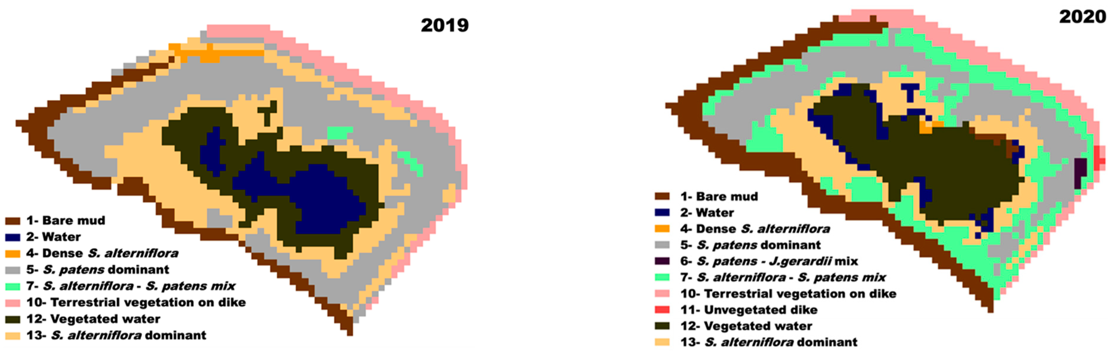
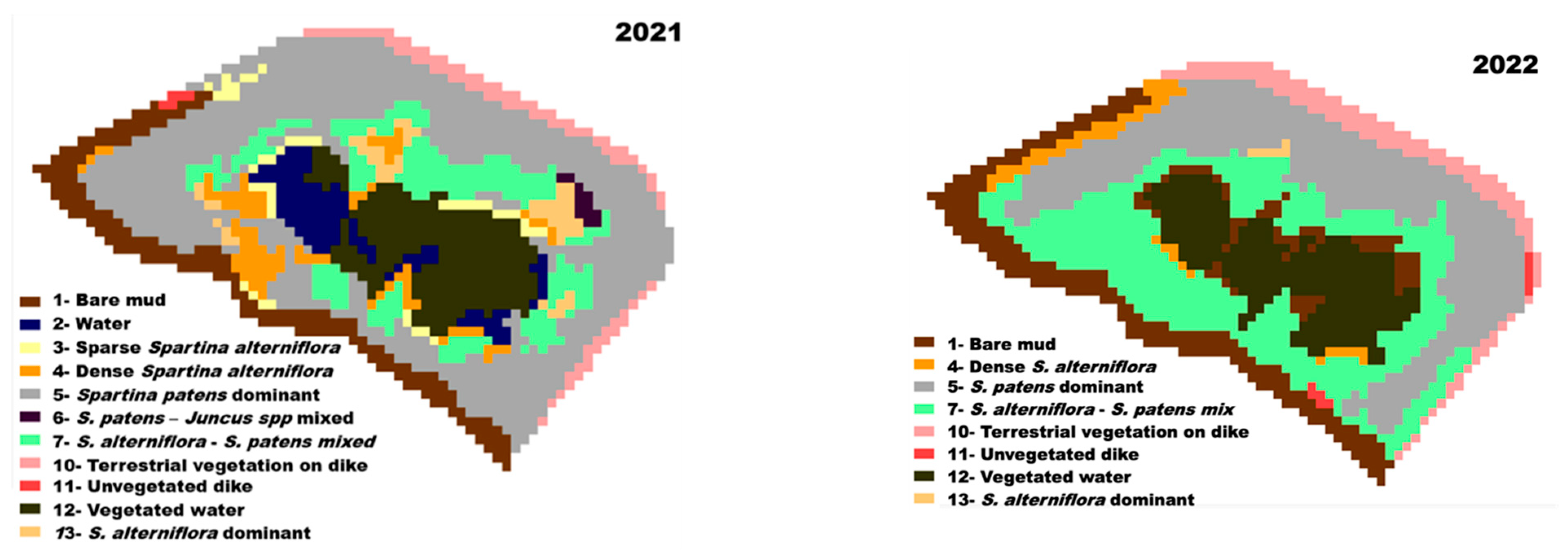
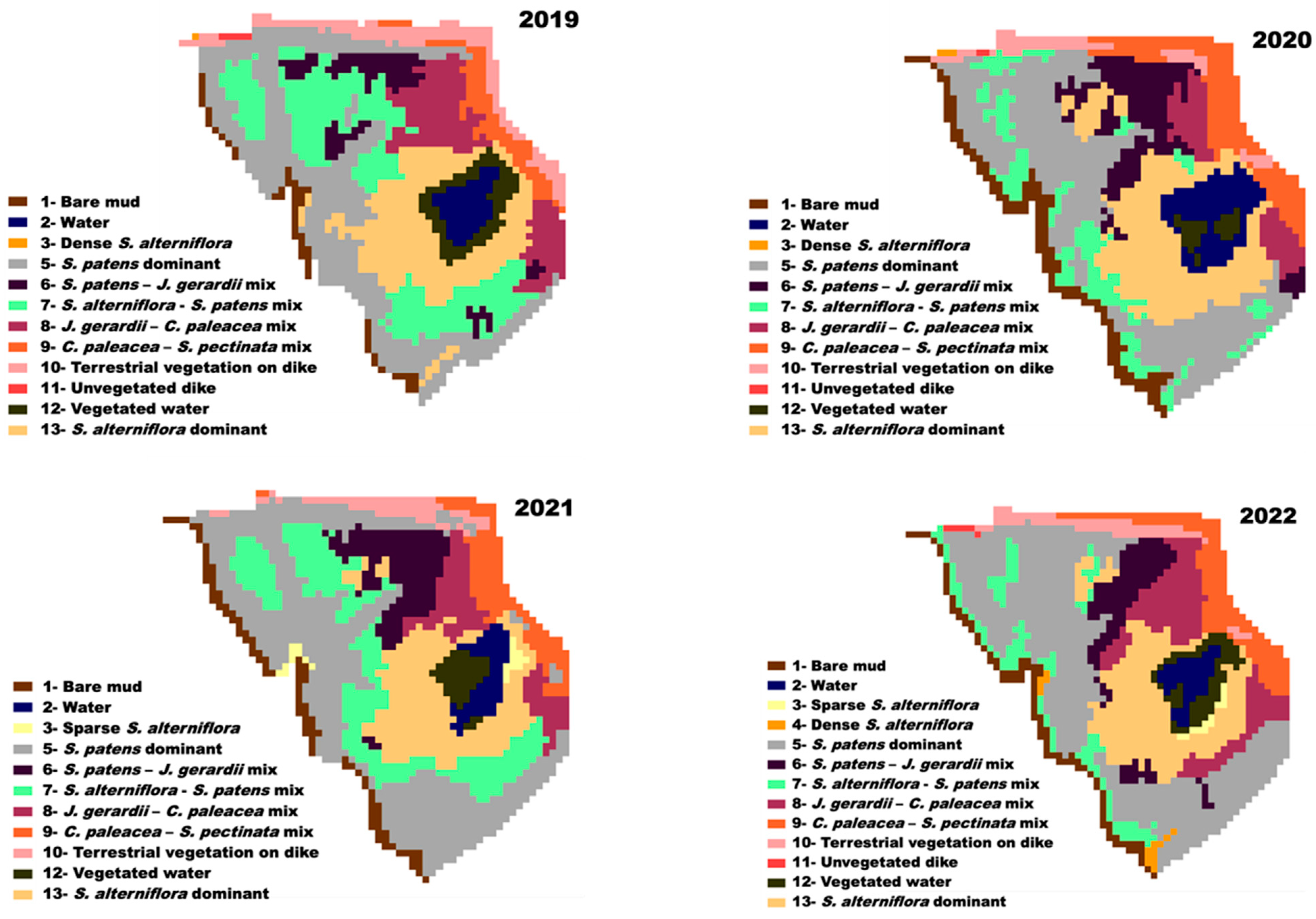
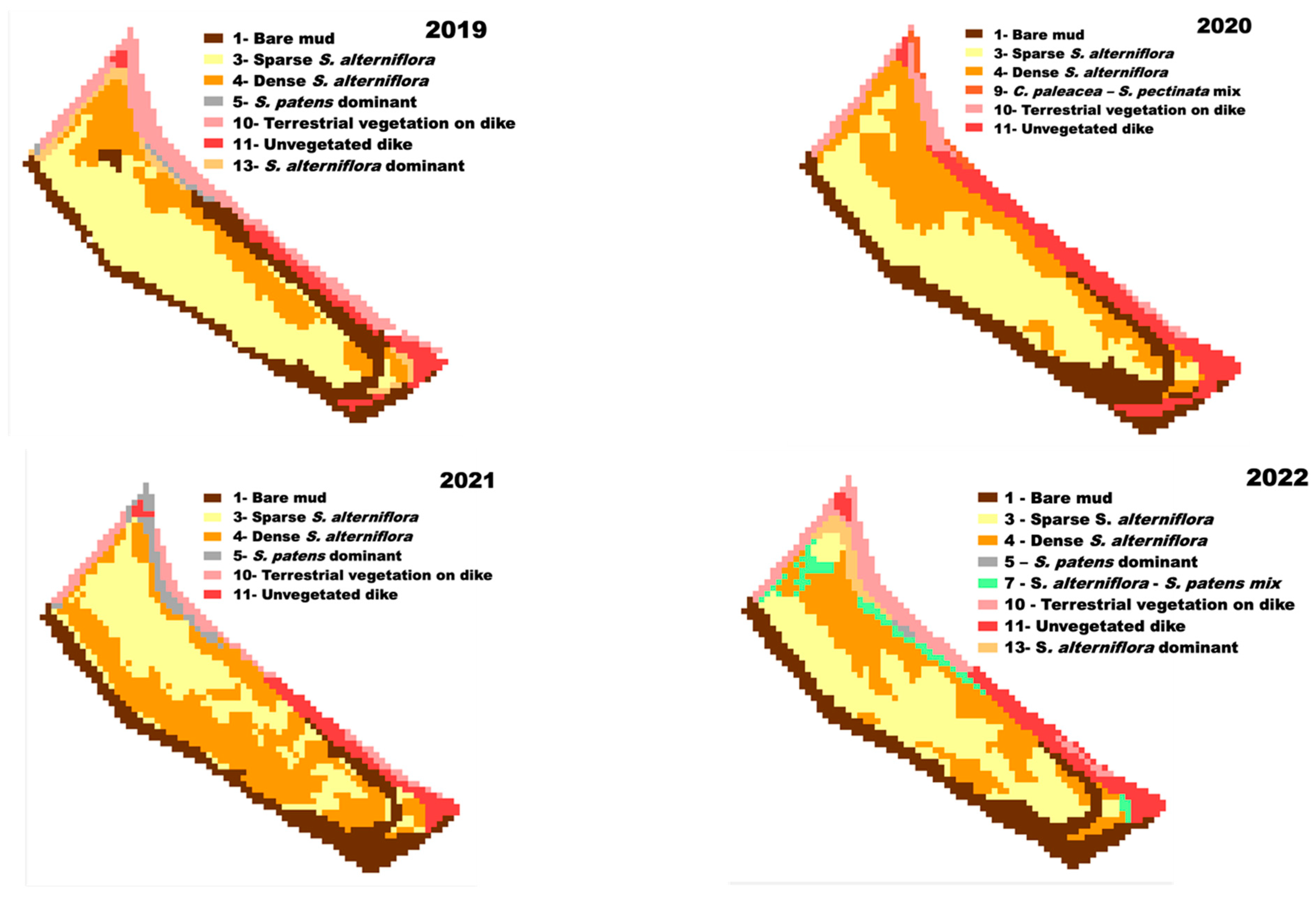
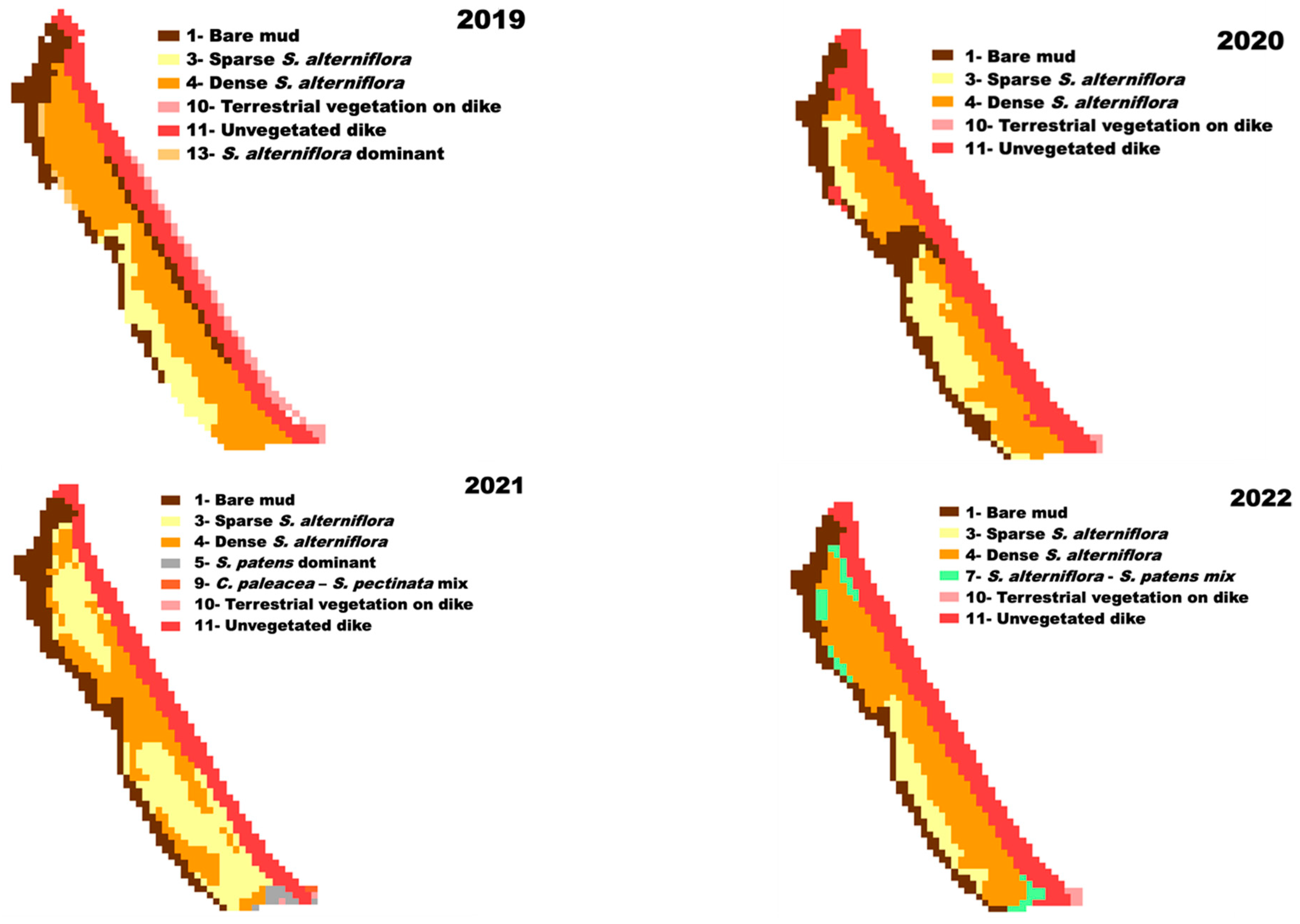
3.5. Landcover Change

The landcover change within and between sites showed spatiotemporal patterns in marsh development that depended on the sites. For both reference sites A and D, about 32% of the total area was occupied by Class 5 (S. patens dominant) consistently across the years (

Table 10. Percent area (%) of each landcover class in the classified image for the reference sites A and D for each year of the study.

Class Number	Site A				Site D
	2019	2020	2021	2022	2019	2020	2021	2022
1	8.39	14.98	9.59	15.44	2.56	6.71	4.33	4.18
2	7.92	3.55	5.55	0.00	3.28	6.31	3.27	2.84
3	0.00	0.00	2.48	0.00	0.00	0.03	1.36	0.64
4	1.18	0.27	5.01	3.06	0.24	0.14	0.03	0.78
5	35.91	20.90	44.26	29.93	27.94	29.00	33.62	36.51
6	0.00	0.43	0.65	0.00	5.23	9.86	7.95	6.80
7	0.75	19.39	12.28	28.71	19.12	10.04	16.48	6.83
8	0.00	0.00	0.00	0.00	9.91	5.14	6.34	10.51
9	0.00	0.00	0.00	0.00	4.60	8.99	6.26	7.83
10	6.22	7.19	4.15	6.76	6.36	3.33	3.02	3.56
11	0.00	0.27	0.26	0.54	0.25	0.11	0.01	0.25
12	15.35	18.80	12.82	15.24	4.01	1.61	2.49	3.52
13	24.29	14.22	2.96	0.32	16.48	18.73	14.83	15.75
TOTAL	100	100	100	100	100	100	100	100

, Figure 3 and Figure 4). This is consistent with the fact that these established sites are mostly high marsh zones [11,51,54]. The main changes in the reference sites involved Classes 5 (S. patens dominant), 7 (S. alterniflora−S. patens mix), and 13 (S. alterniflora dominant), likely influenced by yearly moisture levels.

At site A, Class 13 (S. alterniflora dominant) was the second largest class area, but it declined from 24.3% in 2019 to less than 1% in 2022. During those years, Class 7 (S. alterniflora−S. patens mix) experienced the opposite trend, by increasing from less than 1% to 28.7%. This change appears due to the gradual draining of the salt pool (personal observation by M.A. Barbeau and G.S. Norris). Such drainage led to the disappearance of Class 2 (Water) by 2022 in site A. In site D, Class 13 (S. alterniflora dominant) also showed some decline, from 16.5% in 2019 to 15.8% in 2022 (Table 10, Figure 4). Class 5 (S. patens dominant) increased to 36.5% and Class 2 (Water) remained at a low 2.8% in 2022. Overall, we observed on site D some drying marsh conditions over the 4 years, but to a much lesser extent than site A. For both reference sites, two restoration landcover classes, i.e., Class 3 (Sparse S. alterniflora) and Class 4 (Dense S. alterniflora), occupied 5% or less across the years. To further understand landcover changes, we pooled Classes 3 and 4 with Class 13, and the result shows that S. alterniflora dominant accounted for 25.5% to 3.4% of the total area (over the years) in site A and 18.9% to 16.2% in site D.

Other patterns include Class 12 (Vegetated water), which occupied 15.3% at site A but was small (~4%) at site D, remaining stable for both reference sites. In site A, Class 2 (Water) changed greatly but not Class 12 (Vegetated water). Class 1 (Bare mud), which increased from 8.4% to 15.2% in site A, was observed along the seaward marsh edge, indicating possible edge erosion. In site D, Class 1 (Bare mud) area was variable but remained under 7% cover. The plant communities growing in the high marsh zone, namely Classes 6 (S. patens−J. gerardii mix), 8 (J. gerardii−C. paleacea mix), and 9 (C. paleacea−S. pectinata mix), only occurred in site D and experienced a slight increase by 2022 (Table 10, Figure 4). This indicates that site D was at a stable phase of advanced progression given its various elevational vegetation communities typical of an established saltmarsh.

For the restoration sites (

Table 11. Percent area (%) of each landcover class in the classified image for the restoration sites B and C for each year of the study.

Class Number	Site B				Site C
	2019	2020	2021	2022	2019	2020	2021	2022
1	18.72	18.82	17.63	18.59	16.55	19.23	18.20	15.16
2	0.00	0.00	0.00	0.00	0.00	0.00	0.00	0.00
3	40.58	35.58	30.01	33.07	11.44	17.75	30.78	9.78
4	18.26	26.45	37.26	24.66	43.07	29.81	26.60	41.17
5	0.87	0.00	3.40	0.33	0.00	0.00	1.50	0.00
6	0.00	0.00	0.00	0.00	0.00	0.00	0.00	0.00
7	0.00	0.00	0.00	4.33	0.00	0.00	0.00	4.75
8	0.00	0.00	0.00	0.00	0.00	0.00	0.00	0.00
9	0.00	0.78	0.00	0.00	0.00	0.00	0.18	0.00
10	11.9	5.04	5.51	8.74	6.13	0.43	0.31	0.72
11	6.38	13.34	6.18	7.77	22.68	32.78	22.43	28.43
12	0.00	0.00	0.00	0.00	0.00	0.00	0.00	0.00
13	3.22	0.00	0.00	2.51	0.14	0.00	0.00	0.00
TOTAL	100	100	100	100	100	100	100	100

, Figure 5 and Figure 6), we were most interested in examining the landcover classes representing the foundational species in recovery dynamics, i.e., the two S. alterniflora classes, Class 3 (Sparse S. alterniflora) and Class 4 (Dense S. alterniflora), as well as the S. patens classes Class 7 (S. alterniflora−S. patens mix) and Class 5 (S. patens dominant). Both sites were dominated by S. alterniflora, the bioengineer species of saltmarshes, at about 58% of the total area (average over the two sites and four years). This is consistent with the field observation of the monoculture of S. alterniflora, which spreads through both clonal and sexual reproduction [11,54]. Note the above average was computed by pooling Class 13 (S. alterniflora dominant, a designed reference class) with Classes 3 and 4 (Sparse and Dense S. alterniflora, designed restoration classes). Class 13 is by definition a reference site class, and its presence in the restoration sites should be further investigated. Based on Table 11, site B initially showed a higher cover of Class 3 (Sparse S. alterniflora), while site C showed a higher cover of Class 4 (Dense S. alterniflora). In site B, Class 3 (Sparse S. alterniflora) decreased by 7.5%, while Class 4 (Dense S. alterniflora) increased by 6.4%. In site C, the two S. alterniflora classes showed variation, but no clear pattern.

Of great interest, we detected on the satellite imagery the introduction of S. patens on the marsh platform within both sites B and C in 2022, as shown by the inclusion of Class 7 (S. alterniflora−S. patens mix). We could already detect S. patens (specifically Class 5, S. patens dominant) along the side of the dike (which is relatively high in elevation), in 2019 for site B and 2021 in site C. However, Class 7 had not been yet detected within the actual sites (on the marsh platform) beyond the dike. The Class 7 observation for 2022 is an indication of the maturing of the restoration sites, namely the start of the conversion of the restoration sites from a low marsh zone to a high marsh zone (dominated by S. patens as observed in the reference sites).

In both restoration sites, all the other vegetation classes had a very low importance and did not change much over the years. Among the non-vegetated classes, Class 1 (Bare mud) is the second most important class in site B and the third most important class in site C in 2019. These sites were mostly bare mud in 2011, i.e., one year after initiation of the restoration process [11], but now are dominated by S. alterniflora, and the bare mud class seemed mostly unchanged in 2019–2022. The two water-related classes (Classes 2 and 12) were not detected on the satellite imagery for both sites in 2019–2022, because salt pools are too small or too narrow to be detected by the 10 m by 10 m Sentinel-2 mage.

A final aspect to examine is whether changes occurred in the established dike landward of the reference sites and the new dike landward of the restoration sites (Table 10 and Table 11, Figure 3, Figure 4, Figure 5 and Figure 6). The two dike classes together (Classes 10 and 11) accounted for only 6.3% and 4.2% of the total area for the reference sites A and D, but much more at 16.2% and 28.5% for the restoration sites B and C (data average over the four years). For the reference sites (Figure 3 and Figure 4), the dike is mostly vegetated with Class 10 (Terrestrial vegetation on dike) at 3–7%, and unvegetated dike (Class 11) at 0.5% or less and seemed fairly stable in area. The restoration sites B and C are narrow, which explains why the dike occupies more space of the total area. Site C (Figure 6) is the narrowest and its dike is less vegetated than that of site B (Figure 5), which could be a coastal protection concern.

4. Discussion

4.1. Classification and Validation Accuracies

When classifying Sentinel-2 imagery over saltmarshes using Random Forests, we obtained high overall classification accuracies, with the highest being for the 2021 classification (96.43%) and the lowest for the 2020 classification (92.37%). The 2021 images were comparatively the least affected by the tidal height at the time of image acquisition, possibly explaining the year with the highest classification accuracy in our study. Conversely, the 2020 image of August, a month typically coinciding with the peak vegetation growth (e.g., [76,77,78]), was affected by tides as high as 12.2 m. Despite this, our validation accuracy results are comparable to those achieved by other studies using Sentinel-2 imagery and the RF classifier (87–92%) [40,42,48]. All the other studies used a lower number of landcover classes (up to 5), while we produced a map with 13 landcover classes. Accuracy typically diminishes with greater numbers of landcover classes. The study in [40] in Table 1 achieved a classification accuracy of 99%, but with only five classes, by using object-based image analysis (OBIA). OBIA was also applied in [44] to produce a map of 10 landcover classes, with a resulting accuracy (93%) like ours, even though they used additional WorldView-2 and -3 images. OBIA can be particularly helpful if the objects of interest are substantially larger than the spatial resolution of pixels [79], which was not the case for our study, and therefore, not a good option. Also contributing to the high accuracy in our study was the use of multi-temporal image classification per year instead of single-temporal image classification, as was already shown in other studies [41,80]. Multi-temporal image classification works particularly well for areas with a strong seasonality [81,82], like our north temperate saltmarshes [54].

Our study’s overall validation accuracy was the highest for 2019 (93.02%) and the lowest for 2022 (89.73%). The lower accuracy in 2022 coincided with an increase in the complexity of the floristic composition of several observation points, in contrast to the previous years. This is the reason why the number of validation points (224) was fewer in 2022, compared to the 301 observation points used in the previous three years (Table 5). As observed in many other studies (e.g., [83]), validation accuracies are lower than classification accuracies because validation accuracies are computed against an independent dataset, while the classification accuracies (i.e., out-of-bag) are computed based on the training data. Without the validation accuracies, one may overestimate the mapping accuracy.

4.2. Insights from the Variable Importance Ranking

Our list of variable importance produced by Random Forests for saltmarsh mapping indicated that the original Sentinel-2 reflectance bands from July and September were more important (top five input features per year) than those of Spring and August. When considering the top 25 input features for all years, the original reflectance bands of the August image also appeared frequently (23% of the time) along with those of the June (20%), July (25%), and September (19%) images. Unsurprisingly, the May input features were infrequent among the top ones, because the dead above-ground plant biomass has mostly been sheared away by ice over the winter, leaving much of the marsh surface denuded in the early to mid-spring, particularly in the low marsh zone. By mid-June, plants mostly emerged from underground roots and rhizomes in Maritime Canadian saltmarshes [11,54], and so June reflectance did appear among the most important input features. Although reflectance images of August were common amongst the topmost important input features, we were surprised that they were not more important than the ones of the July image; most plants (dominated by graminoids) in our saltmarshes are fully grown and are flowering in August, whereas they are still growing and mostly not yet flowering in July [54,84]. Our sister project using drone remote sensing of the Aulac saltmarshes found that August input features were more important than the July ones [59]. As briefly alluded to above, we suggest some caution in our result about the input features of the August images. Indeed, the satellite images for both 2019 and 2020 was obtained when the tide was quite high (>12 m), leading to the inundation of the restoration sites, while the reference sites had the plant canopy in the high marsh zone above water and were very visible (Supplementary Table S12). Note that our August images for 2021 and 2022 were obtained when the tide was very low and were not affected by tidal inundation. In a study about saltmarsh vegetation mapping in China using Sentinel-1 SAR and Sentinel-2 images, [43] also observed that input features of the September image were important. Furthermore, this study showed that September images allowed to separate spectrally the various species of the marsh, including Spartina alterniflora. One reason is that plant senescence affects the spectral response of the vegetation. In Maritime Canada, S. alterniflora has fully developed seeds by early to mid-September and starts to senesce soon after in September [84,85]. These phenological developments late in (and at the end of) the growing season for S. alterniflora as well as other common saltmarsh graminoids, such as Spartina patens, Juncus gerardii, and Carex paleacea, occur at slightly different times and with different spectral characteristics, which can be used in vegetation mapping by satellite imagery. Among all the original Sentinel-2 reflectance bands, SWIR-2 (2190 nm) and SWIR-1 (1610 nm) were consistently ranked in the top 10 most important reflectance bands in our yearly classifications. Both reflectance bands are related to the leaf water content [86]. Given that saltmarsh plants are characterized by zonal elevations with varying levels of inundation, the SWIR-1 and SWIR-2 are expected to be most useful to distinguish the plants based on their water content. These results are not in agreement with [43], who observed that the blue and red reflectance bands were more important than the SWIR bands.

The Sentinel-2 image classification results also showed that, among the 25 top input features, vegetation indices were less important (30%) than raw reflectance bands (70%). Our sister study of the Aulac saltmarshes using drone imagery [59] also found that vegetation indices were not necessarily better than the reflectance bands. In our study, the most important vegetation indices for the years of 2019, 2020, and 2022 were NR, NNIR, and RVI, which use near-infrared and red reflectance. RVI was also ranked in the top three most important features by [43]. The other studies using RF only considered two vegetation indices, NDVI and NDWI (Normalized Difference Water Index), which is based on near-infrared (NIR) and shortwave infrared (SWIR) reflectances [40,44,47]. We did not consider NDWI because we aimed to focus on vegetation classification, not water body detection or assessing vegetation water stress.

4.3. Landcover Change and Assessment of Saltmarsh Recovery

Our satellite imagery-based methodology enabled us to assess the state of saltmarshes undergoing restoration for about a decade, as well as the state of reference saltmarshes. An important pattern detected in the Aulac restoration sites was the beginning conversion from a low marsh zone to conditions more representative of a high marsh zone. This conversion began with the initial colonization and spread of S. patens in 2017 [54]. At the time, these patches were few and small, but we are now able to detect them on the 2019–2022 satellite imagery, indicating that the marsh is maturing. As a result, we observed an increase in the area (4%) of S. patens−S. alterniflora mix (Class 7) in the restoration sites (i.e., beyond the higher elevation dike). It is useful to know that it took 3 years (from 2019 to 2022) for satellite imagery to detect this. This is valuable information about the lag between the time when an important recovery dynamic starts on the ground and the time when it can be detected on satellite imagery.

An earlier pattern that we have been following on the ground in the restoration sites [54] and that we detected on the classified images is the shift between the two phenotypes (tall form and short form) of S. alterniflora. Both phenotypes are partly the result of environmental conditions [86]. Tall-form S. alterniflora occurs in lower elevation and more inundated areas like young restoration marshes and creek banks in established marshes. It typically has looser stem density and more leaf area per plant, with numerically more and longer leaves. As the saltmarsh surface accretes during recovery, it experiences less flooding and nutrient replenishment, leading S. alterniflora to exhibit a short-form phenotype compared to the previously observed tall form [2,54,85]. Short-form S. alterniflora has tighter stem density but less leaf area per plant than the tall-form, which may or may not make the ground beneath more visible from above. We suspect that the generally decreasing Class 3 (Sparse S. alterniflora) and increasing Class 4 (Dense S. alterniflora) reflects a change from tall-form S. alterniflora with looser stem density to short-form S. alterniflora with tighter stem density in the restoration sites.

Additionally, we know that the two restoration sites (sites B and C) have an elevational difference that would impact the rate of vegetation progression over time. Restoration site C (which is on average 102 cm lower than reference site D as of 2021) is lower in elevation than restoration site B (which is on average 86 cm lower than reference site D) (J. Ollerhead, unpublished data). This implies that site C may have a more persistent community of S. alterniflora, while site B conditions may facilitate a faster spread of S. patens and so an earlier conversion to a high marsh zone. As of 2022, and mentioned above, both sites B and C have evidence of S. patens mixed in with S. alterniflora (Class 7). Before that, site B showed a higher S. patens (Class 5) presence along and near its dike edge than site C, perhaps reflecting its greater elevation than site C and readiness for conversion to a high marsh zone. While the restoration sites are showing signs of progressing towards a mature saltmarsh community, they have a relatively narrow width (~100 m) between the seaward marsh edge and the realigned dike. This is concerning because the sites might not have suitable space to accommodate the different vegetative zonal elevational patterns, which are characteristic of a mature saltmarsh, particularly if marsh edge erosion is faster than the accretion and development of the young saltmarsh [39]. This may prove to be a problem, and so, the landward dike may need to be realigned further inland. In their assessment of dikes throughout Maritime Canada, [87] showed that the dikes’ vulnerability to seawater overtopping is rising, and this is closely connected to the probability of the loss of the foreshore saltmarsh (which helps protect the dikes) if it is too narrow. Our landcover maps show that both Aulac restoration sites B and C can accommodate for the S. patens and S. alterniflora mix (Class 7) and eventually hopefully the S. patens dominant (Class 5) landcover. Our analysis of the landward dike of the restoration sites indicated that the dike area has not changed and was generally well-vegetated, in 2019–2022. However, for a resilient saltmarsh ecosystem that is able to host diverse faunal and floral species and provide the best coastal protection, the presence of high marsh plant species such as J. gerardii, C. paleacea, Bolboschoenus maritimus, and Spartina pectinata is important. Overall, our classified images provide useful information by showing evidence that the saltmarshes have been accreting (based on the vegetation communities observed), but also that they are subject to natural disturbances and erosion.

While clear signs of maturation were observed in the restoration sites, the reference sites had varying patterns. Reference site D was stable over the 2019–2022 period. Reference site A, on the other hand, experienced a change in landcover due to the gradual draining of the large central salt pool. This draining was likely affected by the erosion of the marsh’s seaward edge that opened a narrow barrier between the marsh edge and the large salt pool. This highlights how saltmarshes are dynamic ecosystems that change even at an established phase of their progression.

4.4. Assessment of Sentinel-2 Imagery for Monitoring Saltmarsh Restoration

To ensure a comprehensive understanding of our research findings in relation to using Sentinel-2 imagery for saltmarsh vegetation mapping, here are several issues that we addressed. Firstly, the nature of our sites being a relatively short sea-to-land width (100–300 m) implied that the vegetation transition zones can be narrow. This, coupled with the presence of mixed growth of typical saltmarsh vegetation classes, poses a challenge to be able to differentiate and identify well landcover classes on satellite images having a 10 m spatial resolution, because of potential spectral mixing. In our study, this was particularly the case for the classes containing the same species present in prominence in more than one class, such as Class 5 (S. patens dominant) and Class 7 (S. alterniflora−S. patens mix), where S. patens was often the common species, particularly in the reference sites. Thus, coastal sites need to be wide enough across the shore for the Sentinel-2 images to perform well. The marsh surface of our restoration sites (100–200 m width) was relatively level, being dominated by S. alterniflora, and so mapped with accuracy. If they were to develop a sloped surface as they aged (particularly our narrower site C), the mapping accuracy may decrease. We suggest that sites narrower than 100 m, particularly if there is an elevational gradient and vegetational change, may not be well mapped using Sentinel-2 imagery, hence the test of UAV imagery in a sister study [59].

Related to the above, Sentinel-2 imagery (with its 10 m resolution) makes it difficult to map heterogeneous vegetation communities, such as those occurring in saltmarshes. For example, we could not map the small patches of S. patens (~5 m diameter) that have started to dot the restoration sites, observed during fieldwork [54]. To mitigate such a risk of overlooking small but important patterns on the ground, an alternative would be to deploy UAVs equipped with a camera having similar bands as Sentinel-2 to allow the detection of small patches, as shown in [59]. The additional use of such a sensor would contribute towards a much higher spatial resolution to fill the gap with Sentinel-2 during the validation step, hence improving accuracies. Similarly, combining the input features of Sentinel-2 with Synthetic Aperture Radar (SAR) data from Sentinel-1 might help to better classify the water-based landcovers, as shown by [43].

Another issue was the selection of Sentinel-2 images aimed to be as close in time to the field observation dates. This was not always feasible due to cloud cover. For example, we could not find a suitable May image for 2019, due to a combination of fog and clouds; so, we used images from June to October for that year. In the end, all our images had cloud-free cover over the study sites for all four years, although cloud cover on the overall images (which included surrounding land in Westmoreland County, New Brunswick, and Cumberland County, Nova Scotia) ranged up to 46%. Thus, our imagery selection resulted in some time gaps between field observations and image dates. Furthermore, we did not have field observations for May, September, or October. However, vegetation communities are relatively spatially static compared to animal communities or fast-growing biofilm communities; so, the time gaps did not result in changes in the vegetation types substantial enough to create mapping errors. Another consideration in selecting satellite imagery over intertidal areas, such as saltmarshes, is tidal inundation. Since established saltmarshes naturally occur in the high tidal frame, between the lowest high tide (during a neap tide) and the highest high tide (during a spring tide) [2,22], most imagery had a low enough tide. Nevertheless, the high tide coincided with our images from June and August 2019, August 2020, and September 2022, when the tidal height was above 12 m. Such high tides flooded the restoration sites (which are ~ 1 m lower in elevation than the reference sites) and the lowest parts of the reference sites. Our classification results were not greatly negatively affected by marsh flooding. We think the small effect of the flooding on the classified images is because (i) the most heterogenous plant communities are in the reference sites, and the imagery of these sites was marginally affected, and (ii) the restoration sites are homogenous, being mostly a monoculture of S. alterniflora, and the flooding in these sites also appears homogenous in the imagery. So, the result for an image classification is somewhat similar. Furthermore, our use of a multi-temporal method, where images from five months were used, helped dilute the effect of the few images acquired when the tide was very high and overall strengthened our classification results compared to if we used single-image classifications. Thus, regarding the issues highlighted in the present paragraph, using multi-temporal imagery has several advantages to help minimize them.

Having replicate sites per site type, as in our Aulac project (with two restoration sites and two reference sites), is an advantage rather than a limitation for studies, enabling one to assess variation in patterns. However, it can also make classification analysis more difficult. Indeed, the two replicate sites per site type were not identical, hindering across-site training and validation. For example, Classes 6 (S. patens−J. gerardii mix), 8 (J. gerardii−C. paleacea mix), and 9 (C. paleacea−S. pectinata mix), which were observed over a small area in site D and barely in site A, are classes that show the transition towards a brackish or terrestrial zone; these classes help to understand how a saltmarsh is maturing from accretion. Such a limited coverage for these classes (and generally only in one site) complicated the training data collection process. Despite the difference between the four sites, we applied a single classification method to the whole study area partly to deal with this issue. An alternative would be to implement separate classifications for each site, but that would impede a direct map comparison between site types and between sites within site types.

Overall, the classification and validation accuracies, and patterns detected showed that our methodology with Sentinel-2 multi-temporal imagery performed very well and we were able to resolve several issues that had appeared. Moving forward our methodology needs to be tested with other coastal marshes along the Bay of Fundy and geographic locations, given each saltmarsh site experiences unique conditions based on tidal amplitude, geomorphology and vegetation composition. Also, developing the best methods for the incorporation of complementary UAV imagery into the methodology would be very useful.

5. Conclusions

Despite the relatively low spatial resolution (10 m) of the Sentinel-2 imagery, it is possible to monitor the restoration trajectory of saltmarshes, as long as they are wide enough (i.e., 100 m or more). By classifying multi-temporal Sentinel-2 images, our study successfully created a map of 13 saltmarsh landcover classes for the vegetation community in the Aulac restoration and reference saltmarshes with an overall classification accuracy of up to 96.43% and an overall validation accuracy of up to 93.35%. Our study methodologically confirmed that Sentinel-2 images, with 12 usable reflectance bands and 10 m spatial resolution, are effective in mapping saltmarsh vegetation communities with good accuracies, if field observations or ancillary data such as UAV or high-resolution images are used in the validation stage. The most important vegetation indices in our classifications were NR and NNIR. Despite time gaps between the field observations of vegetation and image acquisition, our 13 landcover class map and multi-temporal imagery offered a robust quantification method. In particular, the method allowed the easier meticulous monitoring of the vegetation dynamics of saltmarshes, compared to the current typical saltmarsh vegetation classifications that use fewer landcover classes (such as simply low, mid, and high marsh zones). Furthermore, we tested the methodology for saltmarshes located in a dynamic environment influenced by extreme tides, high winds, and winter disturbance, namely the upper Bay of Fundy. Generalizing the method to saltmarshes located in other geographic locations may require adapting the method to other tidal systems.

From the classified images, we then could observe useful site dynamics. The restoration sites B and C were in the early development phase and showed positive signs of recovery, mainly accretion based on the introduction of S. patens amongst S. alterniflora. Despite a small elevational difference, both restoration sites have about the same percent cover of S. patens−S. alterniflora mix (Class 7) as of 2022. However, we predict that the lower elevation site C will show a longer-lasting community of S. alterniflora (low marsh zone), before converting to a high marsh zone dominated by S. patens, if the accretion rate stays relatively the same. Generally, we expect that the restoration sites will gradually transition from sparse and dense S. alterniflora (Class 3 to Class 4) to S. alterniflora−S. patens mix (Class 7) and eventually S. patens dominant (Class 5). The reference sites showed differences in the assemblage of high marsh species and the size of their salt pools. The different moisture levels in the soil around the perimeter of the salt pools/depressions were likely determinants of the plant succession patterns. We predict that site A will continue to have drying conditions in the salt pool depressions, which will be colonized by S. alterniflora dominant (Class 13). The areas around that pool will transition from S. alterniflora dominant to the S. alterniflora−S. patens mix (Class 7) to eventually become S. patens dominant. Moreover, the landward dike, whose structural integrity is a crucial component in protecting the farmlands adjacent to the saltmarshes, was well-covered with terrestrial vegetation and generally stable for both the reference and restoration sites.

In summary, our study contributes to the knowledge that saltmarsh recovery is a long-term process from the initial stages until full recovery and shows the usefulness of Sentinel-2 images to accurately monitor saltmarsh vegetation changes. The developed methodology based on the utilization of Sentinel-2 images is a valuable tool for assessing the current and future state of saltmarshes in the Bay of Fundy, both established and under restoration, as well as in other north temperate locations. This is important at a time when conservation and restoration initiatives are increasingly being implemented [27,28].

References

1. Mitsch, W.J.; Gosselink, J.G. Wetlands, 5th ed.; Van Nostrand Reinhold: New York, NY, USA, 2015; 747p. [Google Scholar]
2. Bertness, M.D. Atlantic Shorelines: Natural History and Ecology; Princeton University Press: Princeton, NJ, USA, 2007; 432p. [Google Scholar]
3. Redfield, A.C. Development of a New England Salt Marsh. Ecol. Monogr. 1972, 42, 201–237. [Google Scholar] [CrossRef]
4. Ford, H.; Garbutt, A.; Ladd, C.; Malarkey, J.; Skov, M.W. Soil Stabilization Linked to Plant Diversity and Environmental Context in Coastal Wetlands. J. Veg. Sci. 2016, 27, 259–268. [Google Scholar] [CrossRef]
5. Gracia, A.; Rangel-Buitrago, N.; Oakley, J.A.; Williams, A.T. Use of Ecosystems in Coastal Erosion Management. Ocean Coast. Manag. 2018, 156, 277–289. [Google Scholar] [CrossRef]
6. Breckle, S.W. Salinity, Halophytes, and Salt-Affected Natural Ecosystems. In Salinity: Environment—Plants—Molecules; Läuchli, A., Lüttge, U., Eds.; Springer: Dordrecht, The Netherlands, 2002; pp. 53–77. [Google Scholar] [CrossRef]
7. Bertness, M.D.; Ellison, A.M. Determinants of Pattern in a New England Salt Marsh Plant Community. Ecol. Monogr. 1987, 57, 129–147. [Google Scholar] [CrossRef]
8. Bertness, M.D. Zonation of Spartina patens and Spartina alterniflora in New England Salt Marsh. Ecology 1991, 72, 138–148. [Google Scholar] [CrossRef]
9. Crain, C.M.; Silliman, B.R.; Bertness, S.L.; Bertness, M.D. Physical and Biotic Drivers of Plant Distribution across Estuarine Salinity Gradients. Ecology 2004, 85, 2539–2549. [Google Scholar] [CrossRef]
10. Ollerhead, J.; Davidson-Arnott, R.G.D.; Scott, A. Cycles of Saltmarsh Extension and Contraction, Cumberland Basin, Bay of Fundy, Canada. In Geomorphologia Littoral I Quaternari: Homenatge al Professor V. M. Rosselló i Verger; Fleury, M., McCann, S.B., Eds.; Servei de Publicacions, Universitat de València: València, Spain, 2005; pp. 293–305. [Google Scholar]
11. Virgin, S.D.S.; Beck, A.D.; Boone, L.K.; Dykstra, A.K.; Ollerhead, J.; Barbeau, M.A.; McLellan, N.R. A Managed Realignment in the Upper Bay of Fundy: Community Dynamics during Saltmarsh Restoration over 8 Years in a Megatidal, Ice-Influenced Environment. Ecol. Eng. 2020, 149, 105713. [Google Scholar] [CrossRef]
12. Buth, G.J.C. Decomposition of Roots of Three Plant Communities in a Dutch Salt Marsh. Aquat. Bot. 1987, 29, 123–138. [Google Scholar] [CrossRef]
13. Artigas, F.; Shin, J.Y.; Hobble, C.; Marti-Donati, A.; Schäfer, K.V.R.; Pechmann, I. Long-Term Carbon Storage Potential and CO2 Sink Strength of a Restored Salt Marsh in New Jersey. Agric. For. Meteorol. 2015, 200, 313–321. [Google Scholar] [CrossRef]
14. Wollenberg, J.T.; Ollerhead, J.; Chmura, G.L. Rapid Carbon Accumulation Following Managed Realignment on the Bay of Fundy. PLoS ONE 2018, 13, e0193930. [Google Scholar] [CrossRef]
15. Pétillon, J.; Potier, S.; Carpentier, A.; Garbutt, A. Evaluating the Success of Managed Realignment for the Restoration of SaltMarshes: Lessons from Invertebrate Communities. Ecol. Eng. 2014, 69, 70–75. [Google Scholar] [CrossRef]
16. Baker, R.; Taylor, M.D.; Able, K.; Beck, M.W. Fisheries Rely on Threatened Salt Marshes. Science 2020, 370, 670–671. [Google Scholar] [CrossRef] [PubMed]
17. Shriver, W.G.; Greenberg, R. Avian Community Responses to Tidal Restoration along the North Atlantic Coast of North America. In Tidal Marsh Restoration: A Synthesis of Science and Management; Roman, C.T., Burdick, D.M., Eds.; Island Press/Center for Resource Economics: Washington, DC, USA, 2012; pp. 119–143. [Google Scholar] [CrossRef]
18. Adam, P. Saltmarshes in a Time of Change. Environ. Conserv. 2002, 29, 39–61. [Google Scholar] [CrossRef]
19. Gedan, K.B.; Silliman, B.R.; Bertness, M.D. Centuries of Human-Driven Change in Saltmarsh Ecosystems. Annu. Rev. Mar. Sci. 2009, 1, 117–141. [Google Scholar] [CrossRef]
20. McOwen, C.J.; Weatherdon, L.V.; van Bochove, J.-W.; Sullivan, E.; Blyth, S.; Zöckler, C.; Stanwell-Smith, D.; Kingston, N.; Martin, C.S.; Spalding, M.; et al. A Global Map of Saltmarshes. Biodivers. Data J. 2017, 5, e11764. [Google Scholar] [CrossRef] [PubMed]
21. Ganong, W.F. The Vegetation of the Bay of Fundy Salt and Diked Marshes: An Ecological Study. Bot. Gaz. 1903, 36, 161–186, 280–302, 349–369, 429–455. [Google Scholar]
22. Thomas, M.L.H. (Ed.) Marine and Coastal Systems of the Quoddy Region, New Brunswick; Canadian Special Publication of Fisheries and Aquatic Sciences; Dept. of Fisheries and Oceans: Ottawa, ON, Canada, 1983; 306p. [Google Scholar]
23. Butzer, K.W. French Wetland Agriculture in Atlantic Canada and Its European Roots: Different Avenues to Historical Diffusion. Ann. Assoc. Am. Geogr. 2002, 92, 451–470. [Google Scholar] [CrossRef]
24. Koohzare, A.; Vaníček, P.; Santos, M. Pattern of Recent Vertical Crustal Movements in Canada. J. Geodyn. 2008, 45, 133–145. [Google Scholar] [CrossRef]
25. Boon, J.D. Evidence of Sea Level Acceleration at U.S. and Canadian Tide Stations, Atlantic Coast, North America. J. Coast. Res. 2012, 28, 1437–1445. [Google Scholar] [CrossRef]
26. Sherren, K.; Ellis, K.; Guimond, J.A.; Kurylyk, B.; LeRoux, N.; Lundholm, J.; Mallory, M.L.; van Proosdij, D.; Walker, A.K.; Bowron, T.M.; et al. Understanding Multifunctional Bay of Fundy Dykelands and Tidal Wetlands Using Ecosystem Services—A Baseline. FACETS 2021, 6, 1446–1473. [Google Scholar] [CrossRef]
27. Waltham, N.J.; Elliott, M.; Lee, S.Y.; Lovelock, C.; Duarte, C.M.; Buelow, C.; Simenstad, C.; Nagelkerken, I.; Classens, L.; Wen, C.C.K.; et al. UN Decade on Ecosystem of Restoration 2021–2030—What Chance for Success in Restoring Coastal Ecosystems? Front. Mar. Sci. 2020, 7, 71. [Google Scholar] [CrossRef]
28. Waltham, N.J.; Alcott, C.; Barbeau, M.A.; Cebrian, J.; Connolly, R.M.; Deegan, L.A.; Dodds, K.; Goodridge Gaines, L.A.; Gilby, B.L.; Henderson, C.J. Tidal Marsh Restoration Optimism in a Changing Climate and Urbanizing Seascape. Estuaries Coasts 2021, 44, 1681–1690. [Google Scholar] [CrossRef]
29. Naojee, S.M.; Leblon, B.; LaRocque, A.; Norris, G.S.; Barbeau, M.A.; Rowland, M. Saltmarsh vegetation mapping in Atlantic Canada using Sentinel-2 imagery. In Proceedings of the 10th International Conference on Agro-Geoinformatics and 43rd Canadian Symposium on Remote Sensing (CSRS), Quebec City, QC, Canada, 12–14 July 2022; Abstracts. p. 2. [Google Scholar]
30. Breiman, L. Random Forests. Mach. Learn. 2001, 45, 5–32. [Google Scholar] [CrossRef]
31. Pal, M. Random Forest Classifier for Remote Sensing Classification. Int. J. Remote Sens. 2005, 26, 217–222. [Google Scholar] [CrossRef]
32. Gislason, P.O.; Benediktsson, J.A.; Sveinsson, J.R. Random Forests for Landcover Classification. Pattern Recognit. Lett. 2006, 27, 294–300. [Google Scholar] [CrossRef]
33. Waske, B.; Braun, M. Classifier Ensembles for Landcover Mapping Using Multitemporal SAR Imagery. ISPRS J. Photogramm. Remote Sens. 2009, 64, 450–457. [Google Scholar] [CrossRef]
34. LaRocque, A.; Leblon, B.; Woodward, R.; Mordini, M.; Bourgeau, L.; Landon, A.; Camill, P. Use of Radarsat-2 and Alos-PalSAR SAR Images for Wetland Mapping in New Brunswick. In Proceedings of the 2014 IEEE International Geoscience and Remote Sensing Symposium (IGARSS 2014), Quebec City, QC, Canada, 13–18 July 2014; pp. 1226–1229. [Google Scholar]
35. He, J.; Harris, J.R.; Sawada, M.; Behnia, P.A. Comparison of Classification Algorithms Using Landsat-7 and Landsat-8 Data for Mapping Lithology in Canada’s Arctic. Int. J. Remote Sens. 2015, 36, 2252–2276. [Google Scholar] [CrossRef]
36. Forsey, D.; LaRocque, A.; Leblon, B.; Skinner, M.; Douglas, A. Refinements in Eelgrass Mapping at Tabusintac Bay (New Brunswick, Canada): A Comparison between Random Forest and the Maximum Likelihood Classifier. Can. J. Remote Sens. 2020, 46, 640–659. [Google Scholar] [CrossRef]
37. Martínez-Prentice, R.; Villoslada Peciña, M.; Ward, R.D.; Bergamo, T.F.; Joyce, C.B.; Sepp, K. Machine Learning Classification and Accuracy Assessment from High-Resolution Images of Coastal Wetlands. Remote Sens. 2021, 13, 3669. [Google Scholar] [CrossRef]
38. Desplanque, C.; Mossman, D.J. Tides and Their Seminal Impact on the Geology, Geography, History, and Socio-Economics of the Bay of Fundy, Eastern Canada. Atl. Geosci. 2004, 40, 1–65. [Google Scholar] [CrossRef]
39. Boone, L.K.; Ollerhead, J.; Barbeau, M.A.; Beck, A.D.; Sanderson, B.G.; McLellan, N.R. Returning the Tide to Dikelands in a Macrotidal and Ice-Influenced Environment: Challenges and Lessons Learned. In Coastal Wetlands: Alteration and Remediation; Finkl, C., Makowski, C., Eds.; Coastal Research Library; Springer: Cham, Switzerland, 2017; Volume 21, pp. 705–749. [Google Scholar] [CrossRef]
40. Kaplan, G.; Avdan, U. Mapping and Monitoring Wetlands Using Sentinel-2 Satellite Imagery. ISPRS Ann. Photogramm. Remote Sens. Spat. Inf. Sci. 2017, 4, 271–277. [Google Scholar] [CrossRef]
41. Sun, C.; Li, J.; Liu, Y.; Liu, Y.; Liu, R. Plant Species Classification in Salt Marshes Using Phenological Parameters Derived from Sentinel-2 Pixel-Differential Time-Series. Remote Sens. Environ. 2021, 256, 112320. [Google Scholar] [CrossRef]
42. Villa, P.; Giardino, C.; Mantovani, S.; Tapete, D.; Vecoli, A.; Braga, F. Mapping Coastal and Wetland Vegetation Communities Using Multi-Temporal Sentinel-2 Data. ISPRS Arch. Photogramm. Remote Sens. Spat. Inf. Sci. 2021, 43, 639–644. [Google Scholar] [CrossRef]
43. Zhang, C.; Gong, Z.; Qiu, H.; Zhang, Y.; Zhou, D. Mapping Typical Saltmarsh Species in the Yellow River Delta Wetland Supported by Temporal-Spatial-Spectral Multidimensional Features. Sci. Total Environ. 2021, 783, 147061. [Google Scholar] [CrossRef] [PubMed]
44. Campbell, A.; Wang, Y. High Spatial Resolution Remote Sensing for Salt Marsh Mapping and Change Analysis at Fire Island National Seashore. Remote Sens. 2019, 11, 1107. [Google Scholar] [CrossRef]
45. Rupasinghe, P.A.; Chow-Fraser, P. Mapping Phragmites Cover Using WorldView 2/3 and Sentinel 2 Images at Lake Erie Wetlands, Canada. Biol. Invasions 2021, 23, 1231–1247. [Google Scholar] [CrossRef]
46. Cawkwell, F.G.; Dwyer, N.; Bartlett, D.; Ameztoy, I.; O’Connor, B.; O’Dea, L.; Hills, J.; Brown, A.; Cross, N.; O’Donnell, M.; et al. Saltmarsh Habitat Classification from Satellite Imagery. In Proceedings of 3rd EARSeL Workshop Remote Sensing of the Coastal Zone, Bolzano, Italy, 7–9 June 2007; p. 12. [Google Scholar]
47. Chen, Y.; He, X.; Xu, J.; Guo, L.; Lu, Y.; Zhang, R. Decision Tree-Based Classification in Coastal Area Integrating Polarimetric SAR and Optical Data. Data Technol. Appl. 2021, 56, 342–357. [Google Scholar] [CrossRef]
48. Zhang, X.; Xu, J.; Chen, Y.; Xu, K.; Wang, D. Coastal Wetland Classification with GF-3 Polarimetric SAR Imagery by Using Object-Oriented Random Forest Algorithm. Sensors 2021, 21, 3395. [Google Scholar] [CrossRef] [PubMed]
49. Hu, Y.; Tian, B.; Yuan, L.; Li, X.; Huang, Y.; Shi, R.; Jiang, X.; Wang, L.; Sun, C. Mapping Coastal Salt Marshes in China Using Time Series of Sentinel-1 SAR. ISPRS J. Photogramm. Remote Sens. 2021, 173, 122–134. [Google Scholar] [CrossRef]
50. Lou, P.; Fu, B.; He, H.; Li, Y.; Tang, T.; Lin, X.; Fan, D.; Gao, E. An Optimized Object-Based Random Forest Algorithm for Marsh Vegetation Mapping Using High-Spatial-Resolution GF-1 and ZY-3 Data. Remote Sens. 2020, 12, 1270. [Google Scholar] [CrossRef]
51. Millard, K.; Redden, A.M.; Webster, T.; Stewart, H. Use of GIS and High-Resolution LiDAR in Salt Marsh Restoration Site Suitability Assessments in the Upper Bay of Fundy, Canada. Wetl. Ecol. Manag. 2013, 21, 243–262. [Google Scholar] [CrossRef]
52. Peterson, P.M.; Romaschenko, K.; Arrieta, Y.H.; Saarela, J.M. A Molecular Phylogeny and New Subgeneric Classification of Sporobolus (Poaceae: Chloridoideae: Sporobolinae). Taxon 2014, 63, 1212–1243. [Google Scholar] [CrossRef]
53. Bortolus, A.; Adam, P.; Adams, J.B.; Ainouche, M.L.; Ayres, D.; Bertness, M.D. Supporting Spartina: Interdisciplinary Perspective Shows Spartina as a Distinct Solid Genus. Ecology 2019, 100, e02863. [Google Scholar] [CrossRef] [PubMed]
54. Norris, G.S.; Virgin, S.D.S.; Schneider, D.W.; McCoy, E.M.; Wilson, J.M.; Morrill, K.L.; Hayter, L.; Hicks, M.E.; Barbeau, M.A. Patch-Level Processes of Vegetation Underlying Site-Level Restoration Patterns in a Megatidal Salt Marsh. Front. Ecol. Evol. 2022, 10, 1000075. [Google Scholar] [CrossRef]
55. Sentinel-2 ESA. Sentinel-2 Mission. European Space Agency (ESA). 2022. Available online: https://sentinel.esa.int/web/sentinel/missions/sentinel-2 (accessed on 25 July 2022).
56. Forkuor, G.; Dimobe, K.; Serme, I.; Tondoh, J.E. Landsat-8 vs. Sentinel-2: Examining the Added Value of Sentinel-2′s Red-Edge Bands to Land-Use and Land-Cover Mapping in Burkina Faso. GISci. Remote Sens. 2018, 55, 331–354. [Google Scholar] [CrossRef]
57. Cui, Z.; Kerekes, J.P. Potential of Red Edge Spectral Bands in Future Landsat Satellites on Agroecosystem Canopy Green Leaf Area Index Retrieval. Remote Sens. 2018, 10, 1458. [Google Scholar] [CrossRef]
58. Claverie, M. Evaluation of Surface Reflectance Bandpass Adjustment Techniques. ISPRS J. Photogramm. Remote Sens. 2023, 198, 210–222. [Google Scholar] [CrossRef]
59. Norris, G.S.; LaRocque, A.; Leblon, B.; Barbeau, M.A.; Hanson, A. Comparing Pixel- and Object-Based Approaches for Classifying Multispectral Drone Imagery of a Salt Marsh Restoration and Reference Site. Remote Sens. 2024, 16, 1049. [Google Scholar] [CrossRef]
60. SNAP. ESA Sentinel Application Platform, Version 8.0. 2022. Available online: https://step.esa.int/main/download/snap-download/ (accessed on 23 June 2022).
61. S1TBX. ESA Sentinel-2 Toolbox, Version 8.0.7. 2022. Available online: https://step.esa.int/main/download/snap-download/ (accessed on 23 June 2022).
62. Pignatale, F.C. Sen2Cor Configuration and User Manual, Ref. S2-PDGS-MPC-L2A-SUM-V2.10 Issue 1. 2021. Available online: https://step.esa.int/thirdparties/sen2cor/2.10.0/docs/S2-PDGS-MPC-L2A-SUM-V2.10.0.pdf (accessed on 22 April 2022).
63. Sripada, R.P.; Heiniger, R.W.; White, J.G.; Meijer, A.D. Aerial Color Infrared Photography for Determining Early In-Season Nitrogen Requirements in Corn. Agron. J. 2006, 98, 968–977. [Google Scholar] [CrossRef]
64. Birth, G.S.; McVey, G.R. Measuring the Color of Growing Turf with a Reflectance Spectrophotometer. Agron. J. 1968, 60, 640–643. [Google Scholar] [CrossRef]
65. Pôças, I.; Calera, A.; Campos, I.; Cunha, M. Remote Sensing for Estimating and Mapping Single and Basal Crop Coefficients: A Review on Spectral Vegetation Indices Approaches. Agric. Water Manag. 2020, 233, 106081. [Google Scholar] [CrossRef]
66. Tucker, C.J. Red and Photographic Infrared Linear Combinations for Monitoring Vegetation. Remote Sens. Environ. 1979, 8, 127–150. [Google Scholar] [CrossRef]
67. Buschmann, C.; Nagel, E. In Vivo Spectroscopy and Internal Optics of Leaves as Basis for Remote Sensing of Vegetation. Int. J. Remote Sens. 1993, 14, 711–722. [Google Scholar] [CrossRef]
68. Villa, P.; Mousivand, A.; Bresciani, M. Aquatic Vegetation Indices Assessment through Radiative Transfer Modeling and Linear Mixture Simulation. Int. J. Appl. Earth Obs. Geoinf. 2014, 30, 113–127. [Google Scholar] [CrossRef]
69. Rouse, J.W.; Haas, R.H.; Schell, J.A.; Deering, D.W. Monitoring Vegetation Systems in the Great Plains with ERTS. In Proceedings of the Third Earth Resources Technology Satellite-1 Symposium, Washington, DC, USA, 10–14 December 1973; NASA SP-351; NASA: Washington, DC, USA, 1974; Volume 1, pp. 309–317. [Google Scholar]
70. Cao, Q.; Miao, Y.; Shen, J.; Yu, W.; Yuan, F.; Cheng, S.; Hang, S.; Wang, H.; Yang, W.; Liu, F. Improving In-Season Estimation of Rice Yield Potential and Responsiveness to Topdressing Nitrogen Application with Crop Circle Active Crop Canopy Sensor. Precis. Agric. 2016, 17, 136–154. [Google Scholar] [CrossRef]
71. Liaw, A.; Wiener, M. randomForest: Breiman and Cutler’s Random Forests for Classification and Regression. Version 4.6-10. 2019. Available online: https://rdrr.io/rforge/randomForest/ (accessed on 25 March 2020).
72. Horning, N. Random Forests: An Algorithm for Image Classification and Generation of Continuous Fields Data Sets. In Proceedings of the International Conference on Geoinformatics for Spatial Infrastructure Development in Earth and Allied Sciences, Osaka, Japan, 9 December 2010; p. 6. [Google Scholar]
73. Strobl, C.; Boulesteix, A.L.; Kneib, T.; Augustin, T.; Zeileis, A. Conditional Variable Importance for Random Forests. BMC Bioinform 2008, 9, 307. [Google Scholar] [CrossRef]
74. Louppe, G.; Wehenkel, L.; Sutera, A.; Geurts, P. Understanding Variable Importances in Forests of Randomized Trees. Adv. Neural Inf. Process. Syst. 2013, 26, 431–439. [Google Scholar]
75. Congalton, R.G. A Review of Assessing the Accuracy of Classifications of Remotely Sensed Data. Remote Sens. Environ. 1991, 37, 35–46. [Google Scholar] [CrossRef]
76. Wang, R.; Gamon, J.A.; Montgomery, R.A.; Townsend, P.A.; Zygielbaum, A.I.; Bitan, K.; Tilman, D.; Cavender-Bares, J. Seasonal Variation in the NDVI–Species Richness Relationship in a Prairie Grassland Experiment (Cedar Creek). Remote Sens. 2016, 8, 128. [Google Scholar] [CrossRef]
77. He, W.; Ju, W.; Jiang, F.; Parazoo, N.; Gentine, P.; Wu, X.; Zhang, C.; Zhu, J.; Viovy, N.; Jain, A.K.; et al. Peak Growing Season Patterns and Climate Extremes-Driven Responses of Gross Primary Production Estimated by Satellite and Process-Based Models over North America. Agric. For. Meteorol. 2021, 298–299, 108292. [Google Scholar] [CrossRef]
78. Duan, H.; Qi, Y.; Kang, W.; Zhang, J.; Wang, H.; Jiang, X. Seasonal Variation of Vegetation and Its Spatiotemporal Response to Climatic Factors in the Qilian Mountains, China. Sustainability 2022, 14, 4926. [Google Scholar] [CrossRef]
79. Blaschke, T. Object-Based Image Analysis for Remote Sensing. ISPRS J. Photogramm. Remote Sens. 2010, 65, 2–16. [Google Scholar] [CrossRef]
80. Zhao, Y.; Feng, D.; Yu, L.; Wang, X.; Chen, Y.; Bai, Y.; Hernández, H.J.; Galleguillos, M.; Estades, C.; Biging, G.S.; et al. Detailed Dynamic Land Cover Mapping of Chile: Accuracy Improvement by Integrating Multi-Temporal Data. Remote Sens. Environ. 2016, 183, 254–271. [Google Scholar] [CrossRef]
81. Henits, L.; Jürgens, C.; Mucsi, L. Seasonal Multitemporal Land-Cover Classification and Change Detection Analysis of Bochum, Germany, Using Multitemporal Landsat TM Data. Int. J. Remote Sens. 2016, 37, 3439–3454. [Google Scholar] [CrossRef]
82. Li, N.; Lu, D.; Wu, M.; Zhang, Y.; Lu, L. Coastal Wetland Classification with Multiseasonal High-Spatial Resolution Satellite Imagery. Int. J. Remote Sens. 2018, 39, 8963–8983. [Google Scholar] [CrossRef]
83. Leblon, B.; LaRocque, A.; Gallant, E.; Clyne, K.; Douglas, A. Eelgrass Bed Mapping with Multispectral UAV Imagery in Atlantic Canada. Int. Arch. Photogramm. Remote Sens. Spat. Inf. Sci. 2022, 43, 649–656. [Google Scholar] [CrossRef]
84. Bärlocher, F.; Moulton, V.D. Spartina alterniflora in Two New Brunswick Salt Marshes. I. Growth and Decomposition. Bull. Mar. Sci. 1999, 64, 299–309. Available online: https://www.ingentaconnect.com/content/umrsmas/bullmar/1999/00000064/00000002/art00010 (accessed on 20 November 2024).
85. Vicaire, L.; Stack Mills, A.M.E.; Barbeau, M.A. Developing Knowledge for Salt Marsh Restoration and Salt Marsh Creation in New Brunswick Using Spartina alterniflora Seedlings. New Brunswick Environmental Trust Fund Final Report. Department of Biology, University of New Brunswick: Fredericton, NB, Canada, 2022; 69p, (Unpublished report). [Google Scholar]
86. Anderson, C.M.; Treshow, M. A Review of Environmental and Genetic Factors That Affect Height in Spartina alterniflora Loisel. (Salt Marsh Cord Grass). Estuaries 1980, 3, 168. [Google Scholar] [CrossRef]
87. van Proosdij, D.; Ross, C.; Matheson, G. Nova Scotia Dyke Vulnerability Assessment; Nova Scotia Federation of Agriculture: Truro, NS, Canada, 2018; 35p, Available online: https://nsfa-fane.ca/wp-content/uploads/2018/08/Nova-Scotia-Dyke-Vulnerability-Assessment.pdf (accessed on 15 September 2023).
Figure 1. Location of the 4 saltmarsh sites in Aulac, New Brunswick, in Sentinel-2 imagery acquired on 3 May 2021. A and D are the reference sites, and B and C the restoration sites.
Remotesensing 16 04667 g001
Figure 2. Flowchart presenting the main image processing steps (input data in purple; image processing in light green, image classifier in pink; results in blue).
Remotesensing 16 04667 g002
Figure 3. Landcover map of reference site A obtained by applying the RF classifier to multi-temporal Sentinel-2 images for 2019, 2020, 2021, and 2022.
Remotesensing 16 04667 g003aRemotesensing 16 04667 g003b
Figure 4. Landcover map of reference site D obtained by applying the RF classifier to multi-temporal Sentinel-2 images for 2019, 2020, 2021, and 2022.
Remotesensing 16 04667 g004
Figure 5. Landcover map of restoration site B obtained by applying the RF classifier to multi-temporal Sentinel-2 images for 2019, 2020, 2021, and 2022.
Remotesensing 16 04667 g005
Figure 6. Landcover map of restoration site C obtained by applying the RF classifier to multi-temporal Sentinel-2 images for 2019, 2020, 2021, and 2022.
Remotesensing 16 04667 g006