MambaHR: State Space Model for Hyperspectral Image Restoration Under Stray Light Interference

Abstract

Hyperspectral Imaging (HSI) excels in material identification and capturing spectral details and is widely utilized in various fields, including remote sensing and environmental monitoring. However, in real-world applications, HSI is often affected by Stray Light Interference (SLI), which severely degrades both its spatial and spectral quality, thereby reducing overall image accuracy and usability. Existing hardware solutions are often expensive and add complexity to the system, and despite these efforts, they cannot fully eliminate SLI. Traditional algorithmic methods, on the other hand, struggle to capture the intricate spatial–spectral dependencies needed for effective restoration, particularly in complex noise scenarios. Deep learning methods present a promising alternative because of their flexibility in handling complex data and strong restoration capabilities. To tackle this challenge, we propose MambaHR, a novel State Space Model (SSM) for HSI restoration under SLI. MambaHR incorporates state space modules and channel attention mechanisms, effectively capturing and integrating global and local spatial–spectral dependencies while preserving critical spectral details. Additionally, we constructed a synthetic hyperspectral dataset with SLI by simulating light spots of varying intensities and shapes across spectral channels, thereby realistically replicating the interference observed in real-world conditions. Experimental results demonstrate that MambaHR significantly outperforms existing methods across multiple benchmark HSI datasets, exhibiting superior performance in preserving spectral accuracy and enhancing spatial resolution. This method holds great potential for improving HSI processing applications in fields such as remote sensing and environmental monitoring.

1. Introduction

Hyperspectral Imaging (HSI) is an advanced imaging technique capable of capturing detailed spectral information across hundreds of continuous bands. HSI’s rich spectral data allow the precise identification of the chemical composition and physical properties of materials, making it widely applicable in fields such as environmental monitoring [1,2], military rescue [3,4], and material analysis [5]. However, in practice, HSI is highly susceptible to external interferences, particularly Stray Light Interference (SLI), which degrades image quality and impacts the accuracy of analysis. SLI is notably severe in environments with strong sunlight or poor optical shielding, such as aerial remote sensing, where atmospheric scattering and solar reflections are prevalent, and in complex military scenarios where unpredictable conditions further exacerbate interference. Such interference reduces both the spatial and spectral accuracy of hyperspectral data, thereby limiting its effectiveness in critical applications. Hardware-based methods, such as optical shielding and system optimization, are frequently used to mitigate SLI. Nevertheless, these techniques face significant limitations, particularly in dynamic environments like aerial or urban monitoring, where scattering and reflections are difficult to fully control [6,7,8,9,10]. Additionally, relying solely on hardware solutions often leads to increased system complexity and higher costs, making them impractical in many situations. Therefore, software-based restoration approaches act as an essential complement to hardware measures, improving data quality while effectively managing system complexity and ensuring cost efficiency.

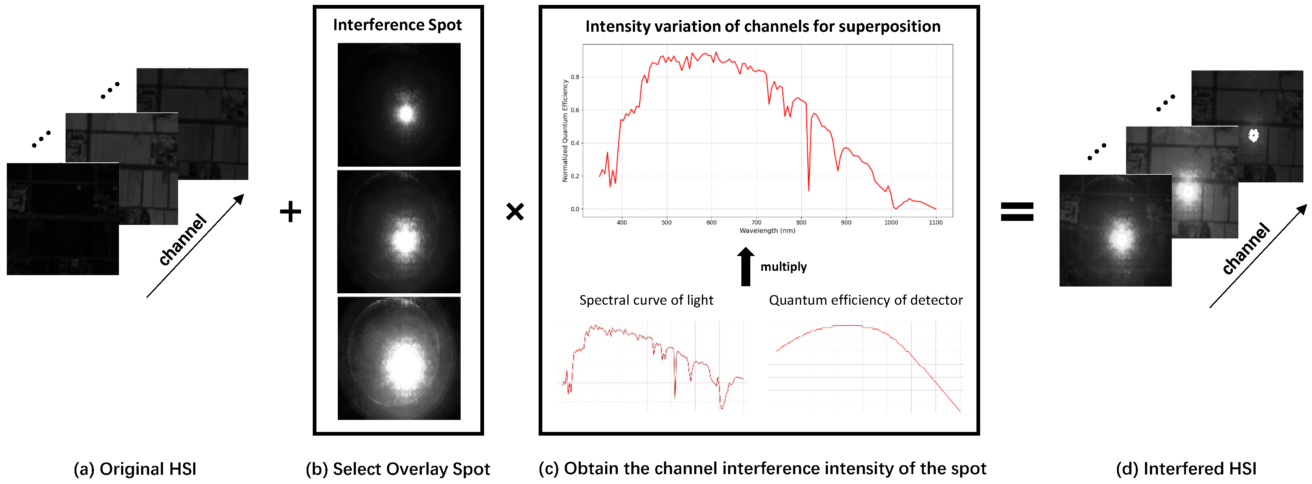
SLI refers to the phenomenon in which light from non-target sources enters the imaging system and is superimposed on the target object’s spectral signals, resulting in data distortion [11,12,13,14]. This issue may arise from flaws in the internal optical system, such as lens reflection, scattering, and stray thermal radiation, or from external sources like sunlight or atmospheric scattering [15]. SLI primarily affects HSIs in two dimensions. In the spatial dimension, it degrades pixel quality, reducing spatial resolution. In the spectral dimension, SLI leads to the overlapping of spectral signals from different wavelengths, distorting the true spectral characteristics of the target object. The simultaneous degradation of spatial and spectral dimensions reduces the accuracy of spectral data interpretation.

Currently, methods to solve the SLI problem can be broadly categorized into hardware-based and software-based approaches. Hardware methods include optimizing optical system design to reduce SLI or employing shielding components and optical filters to block unwanted light [6,7,8,9,10,16,17,18]. Although effective, these hardware approaches often increase system complexity and cost and may not fully eliminate SLI in complex environments. Traditional algorithmic approaches, such as sparse representation and low-rank matrix decomposition, have been widely applied to Hyperspectral Image restoration due to their ability to leverage structural priors [19,20]. However, these methods often struggle to capture the complex spatial–spectral interactions and nonlinear interference patterns commonly found in real-world SLI scenarios. In contrast, deep-learning-based restoration methods offer greater flexibility and superior performance in handling high-dimensional and complex data.

In recent years, deep learning has achieved significant progress in image processing and restoration, particularly in handling high-dimensional and complex data [21,22]. By training neural networks, systems can automatically extract spatial and spectral features, learn the characteristics of SLI, and effectively restore degraded images during inference. Compared to traditional rule-based or statistical restoration methods, deep learning is better suited to handle complex and dynamic scenarios [23]. The main deep learning architectures currently used for HSI restoration include Convolutional Neural Networks (CNNs) and Transformer [24]. CNNs excel at capturing local features, particularly in extracting spatial and spectral dependencies. However, CNNs struggle to capture long-range dependencies, making them less effective in handling images severely affected by SLI. In contrast, Transformer models, which utilize self-attention mechanisms, excel at capturing long-range dependencies, making them ideal for tasks requiring global context. Yet, since the computational complexity of Transformers grows quadratically with data dimensions, applying them to high-dimensional hyperspectral data incurs significant computational costs. To address the limitations of both CNNs and Transformers, State Space Models (SSMs) have recently emerged in HSI processing [25,26]. SSMs are mathematical models that describe system state evolution over time. They express system dynamics through relationships between state and observation variables and are widely used in control theory, signal processing, and time series analysis. In image processing, compared to other models, SSM-based methods offer lower computational complexity when processing high-dimensional data and can more efficiently capture long-range dependencies. Mamba is among the most advanced models developed using SSM. However, the original Mamba was designed for 2D image restoration and lacks the ability to learn spectral dependencies across channels in 3D HSIs. This limitation makes it less effective in handling the complex spatial–spectral relationships required for accurate HSI restoration, especially under challenging conditions such as SLI.

Building on this foundation, we propose MambaHR, a novel method specifically designed for HSI restoration under SLI. MambaHR employs a U-shaped architecture that integrates multi-scale feature extraction. The MambaHR architecture utilizes a 2D-SSM as the core of its spatial attention mechanism, responsible for extracting and processing two-dimensional spatial features. To enhance spectral information capture, MambaHR incorporates a channel attention mechanism, ensuring the accurate restoration of distorted spectral features.

To effectively evaluate MambaHR’s performance in complex interference scenarios, we constructed a synthetic hyperspectral dataset with SLI. This dataset simulates HSIs with varying SLI intensities, reflecting real-world conditions and testing the model’s restoration capabilities under different levels of interference. Experimental results demonstrate that MambaHR achieves superior performance on multiple hyperspectral benchmark datasets, effectively recovering blurred spatial information and correcting spectral distortions.

In summary, the main contributions can be outlined as follows:

• We advance the field of HSI restoration by applying deep learning techniques, incorporating transfer learning, to restore HSIs under SLI.
• We propose MambaHR, an improved version of the original Mamba model, which integrates multi-scale feature extraction with a channel attention mechanism. This enables MambaHR to capture spectral dependencies across channels, overcoming Mamba’s limitations in 3D HSI restoration and significantly enhancing spectral fidelity and spatial detail under SLI.
• We simulate real-world interference conditions and create a synthetic hyperspectral dataset with SLI, establishing a new benchmark for HSI restoration research.

2. Related Work

2.1. Application of Hyperspectral Image Restoration

HSI restoration refers to the application of algorithms or technical methods to repair damaged, degraded, or interfered-with hyperspectral data, aiming to restore its original spectral and spatial accuracy. Restoration tasks encompass denoising, super-resolution, and spectral reconstruction.

In early studies, traditional image processing algorithms, such as sparse representation [27] and low-rank matrix decomposition [28], were widely used. For instance, Zhao et al. [29] proposed an HSI denoising method based on low-rank and sparse models, utilizing a deep unfolding network to enhance denoising efficiency while preserving physical interpretability and generalization. However, as hyperspectral data complexity increases, traditional algorithms have become inadequate for managing global dependencies and capturing intricate spectral–spatial interactions, particularly with high-dimensional data and in complex scenes.

In recent years, deep learning methods have made significant progress in the field of HSI restoration, with CNNs and Transformer [24,30] techniques becoming mainstream tools. CNNs were among the earliest deep-learning techniques widely applied to HSI restoration. By leveraging local perception and multi-layer feature extraction capabilities, CNNs have been particularly effective in image-processing tasks. Maffei et al. [31] proposed a CNN-based HSI denoising method that enhances denoising performance by utilizing spectral and spatial information, significantly outperforming traditional methods. Sidorov et al. [32] introduced a CNN-based method for HSI denoising, restoration, and super-resolution that, without requiring training data, directly utilizes CNN’s inherent properties, achieving results comparable to those of trained networks. Shi et al. [33] proposed two CNN-based HSI reconstruction models, HSCNN-R and HSCNN-D, which leverage residual and dense blocks to significantly enhance the reconstruction performance of HSIs from RGB images. However, CNNs have limitations, particularly in capturing long-range spatial dependencies, and their effectiveness in scenarios with strong global interference is limited.

Transformer models, with their self-attention mechanism, excel in capturing long-range dependencies and have demonstrated outstanding performance in HSI restoration. For super-resolution, Chen et al. [34] proposed MSDformer, which integrates multi-scale spectral attention with deformable convolution Transformer modules to improve both local and global feature extraction. Zhang et al. [35] introduced TD-SAT, a three-dimensional spatial–spectral attention Transformer model for HSI denoising, which incorporates multi-head spectral attention, gated convolution networks, and spectral enhancement modules to effectively remove noise while preserving important spectral and spatial information. Cai et al. [36] proposed MST++ [36], a Transformer-based HSI spectral reconstruction method that progressively improves reconstruction quality through multi-stage spectral attention blocks. This method won first place in the NTIRE 2022 Spectral Reconstruction Challenge. Despite their advantage in capturing global information, Transformers suffer from exponential increases in computational complexity as data dimensions grow, resulting in high computational costs in practical applications.

Recently, SSMs [25,37] have emerged in the field of HSI restoration. Gu et al. [26] proposed Mamba, which captures long-range dependencies through SSM while maintaining low computational complexity, addressing the limitations of both CNN and Transformer models. In denoising tasks, Fu et al. [38] introduced SSUMamba, an HSI denoising method based on SSM, which efficiently captures long-range dependencies while reducing memory consumption through the spatial–spectral continuous scanning mechanism. Dong et al. [39] proposed DHM, which integrates dual spectral S4 blocks to combine global long-range dependencies and local context, yielding excellent performance in HSI reconstruction.

Despite significant progress made by deep learning methods in HSI restoration, research on mitigating SLI remains limited. Effectively restoring spectral and spatial information under complex lighting interference remains a challenge that warrants further investigation.

2.2. Hyperspectral Image Restoration Under Stray Light Interference

The occurrence of SLI in HSI significantly impacts the accuracy of spectral and spatial information. Methods for addressing this interference can be categorized into two types: hardware solutions and algorithm-based software solutions.

In hardware-based methods, researchers often mitigate SLI by refining optical system designs or incorporating specialized filters [6,7,8,9,10]. For example, Lü et al. [10] implemented stray light suppression through a catadioptric space camera optical system design. However, such hardware solutions are often costly and complex to implement and may not fully eliminate interference in dynamic, real-world environments.

In terms of software solutions, current research on SLI mitigation in HSI restoration remains limited. Since SLI generally manifests as complex, global interference with nonlinear and dynamic characteristics, traditional algorithms (such as sparse representation and low-rank decomposition) often struggle to effectively manage the intricate spectral–spatial interactions. Deep learning methods have increasingly been applied to mitigating SLI, leveraging the powerful feature extraction capabilities of neural networks and their ability to capture nonlinear relationships [40,41]. For instance, Li et al. [42] suppressed background stray light in astronomical images using CNNS, significantly reducing its impact in complex astronomical scenes. Zhang et al. [43] employed reinforcement learning techniques to adaptively adjust optical system parameters, reducing SLI under varying illumination conditions and demonstrating strong dynamic adaptability.

Despite the notable progress achieved by deep learning methods in specific scenarios, most approaches are optimized for particular applications, with model training and adjustments tailored to specific types of interference in those scenarios. As a result, when faced with more complex SLI patterns or dynamic environments, these methods often struggle to maintain adaptability and robustness. To address this challenge, we combine innovative dataset construction with novel algorithmic design, aiming to enhance the restoration capacity of HSIs under complex SLI conditions.

3. Methodology

In this section, we introduce the proposed MambaHR architecture, a selective SSM designed for HSI restoration under strong light interference. The model efficiently captures and integrates both spatial and spectral information from HSIs through multi-scale feature extraction and attention-based modules.

3.1. Preliminaries: State Space Models

Recent advancements in structured state-space sequence models, especially the S4 model [25], have significantly driven the development of continuous linear time-invariant systems. These systems map a one-dimensional input sequence $x\left(t\right)\in {\mathbb{R}}^L$ to an output sequence $y\left(t\right)\in {\mathbb{R}}^M$ through an implicit latent state $h\left(t\right)\in {\mathbb{R}}^N$. Formally, the system can be described by the following ordinary differential equation (ODE):

$$h^{\prime }\left(t\right)=Ah\left(t\right)+Bx\left(t\right),$$

(1)

$$y\left(t\right)=Ch\left(t\right)+Dx\left(t\right),$$

(2)

where $h\left(t\right)$ represents the hidden state, and the matrices $A\in {\mathbb{R}}^{N\times N}$, $B\in {\mathbb{R}}^{N\times L}$, $C\in {\mathbb{R}}^{M\times N}$, and $D\in {\mathbb{R}}^{M\times L}$ are the model parameters. The evolution of the hidden state $h\left(t\right)$ depends on the current input $x\left(t\right)$ and the previous hidden state $h(t-1)$, while the output $y\left(t\right)$ is generated from both $h\left(t\right)$ and $x\left(t\right)$.

To implement this in practical deep learning scenarios, the continuous ODE needs to be discretized. A commonly used method for discretization is the zero-order hold rule, which results in

$$\overline{A}=exp(\Delta A),$$

(3)

$$\overline{B}={(\Delta A)}^{-1}(exp\left(A\right)-I)\Delta B,$$

(4)

where $\Delta$ is the sampling step. After discretization, these equations can be rewritten in a form similar to Recurrent Neural Networks (RNNs):

$$h_k=\overline{A}{h}_{k-1}+\overline{B}{x}_k,$$

(5)

$$y_k=C{h}_k+D{x}_k.$$

(6)

Additionally, the discretized equations can be further transformed into a convolutional form to enable more efficient computation:

$$y=x\ast \overline{K},$$

(7)

where $\overline{K}=(C\overline{B},C\overline{A}\overline{B},C{\overline{A}}^2\overline{B},\dots ,C{\overline{A}}^{k-1}\overline{B})$ is the convolutional kernel, ∗ denotes the convolution operation, and k is the sequence length.

Gu et al. introduced the Mamba method [26], which optimizes parameters using a selective scan mechanism, along with hardware-aware strategies to ensure efficient implementation in real-world applications. We applied the Mamba method and further explored its potential applications in spatial–spectral modeling of 3D images.

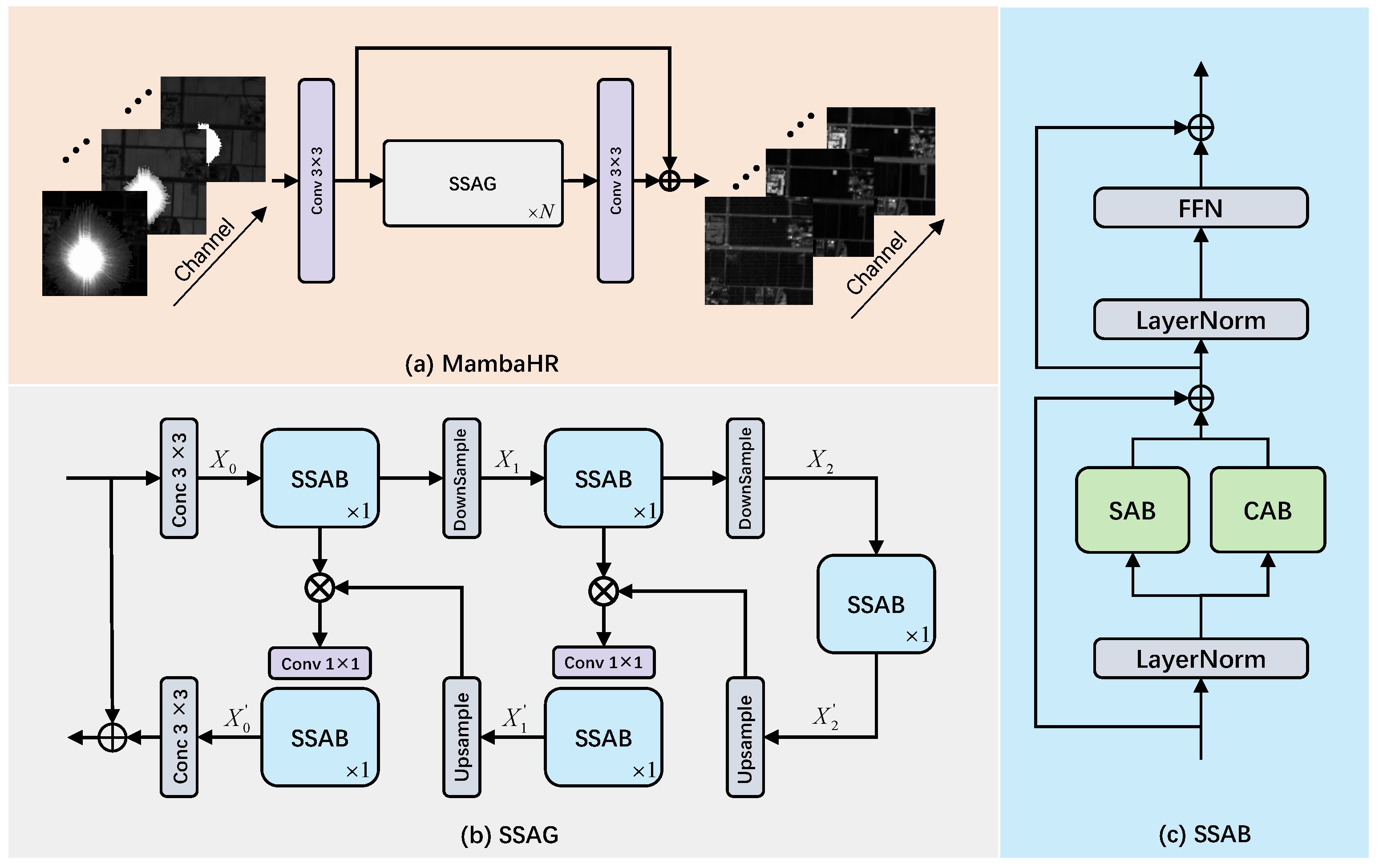
3.2. Overall Architecture

For a given hyperspectral input image $I_{LR}$ with interference, where the image has dimensions $H\times W\times N$, H and W represent the height and width of the image, and N represents the number of spectral channels. A 3 × 3 convolution operation is initially applied to map the input to initial features $F_{init}$, as shown in Figure 1:

$$F_{init}=H_{conv3\times 3}\left(I_{LR}\right),$$

(8)

where $H_{conv3\times 3}$ represents the initial convolution operation.

Subsequently, the initial features are input into N Spatial–Spectral Attention Groups (SSAGs). Each SSAG comprises multiple Spatial–Spectral Attention Blocks (SSABs), which are responsible for refining the input features. Within each SSAG, the features undergo a downsampling process to reduce the spatial dimensions, followed by an upsampling process to restore these dimensions, thereby achieving multi-scale feature fusion. The integration of downsampling, upsampling, and convolution layers enables the model to effectively capture both spatial and spectral information across various scales. Residual connections are utilized to enhance information flow, ensuring that crucial feature details are preserved throughout the deep network, as illustrated in Figure 1. The overall process for each SSAG can be expressed as follows:

$$F_{df}^{\left(i\right)}=H_{SSAG}^{\left(i\right)}\left(F_{init}^{\left(i\right)}\right),i=1,2,\dots ,N$$

(9)

where $H_{SSAG}^{\left(i\right)}$ represents the operations within the i-th SSAG module. Each SSAG contains a series of downsampling, upsampling, and convolution operations.

The SSAB serves as the fundamental component within each SSAG. The SSAB integrates both spectral attention and channel attention, which are responsible for capturing critical spatial and spectral information. It employs residual connections and layer normalization (LayerNorm) to facilitate stable feature propagation, thereby further enhancing feature representation. The specific mechanisms underlying spectral attention and channel attention will be elaborated upon in subsequent sections.

After passing through multiple SSAG modules, the final output features are processed by a convolution layer and added to the initial shallow features $F_{init}$. This residual connection ensures that the original shallow features are preserved in the final output, while deep features are effectively enhanced, as shown in Figure 1. The final output is given by

$$F_{output}=F_{init}+H_{conv}\left(F_{df}^{\left(N\right)}\right),$$

(10)

where $H_{conv}$ is the final convolution operation, and $F_{df}^{\left(N\right)}$ represents the deep features processed by the last SSAG.

This residual connection allows the model to retain the original shallow information while enhancing key feature details through deep convolution operations.

Overall, the MambaHR architecture utilizes a selective SSM for HSI restoration under SLI, integrating contemporary mainstream approaches to image restoration. It effectively extracts and aggregates spatial and spectral information through a combination of downsampling, upsampling, and convolutional layers across multiple SSAG modules. The attention mechanisms within the SSABs further refine the spatial and spectral details, ensuring a balance between the retention of the original information and the enhancement of critical features, as detailed in Section 3.3 and Section 3.4.

3.3. Spatial Attention Block

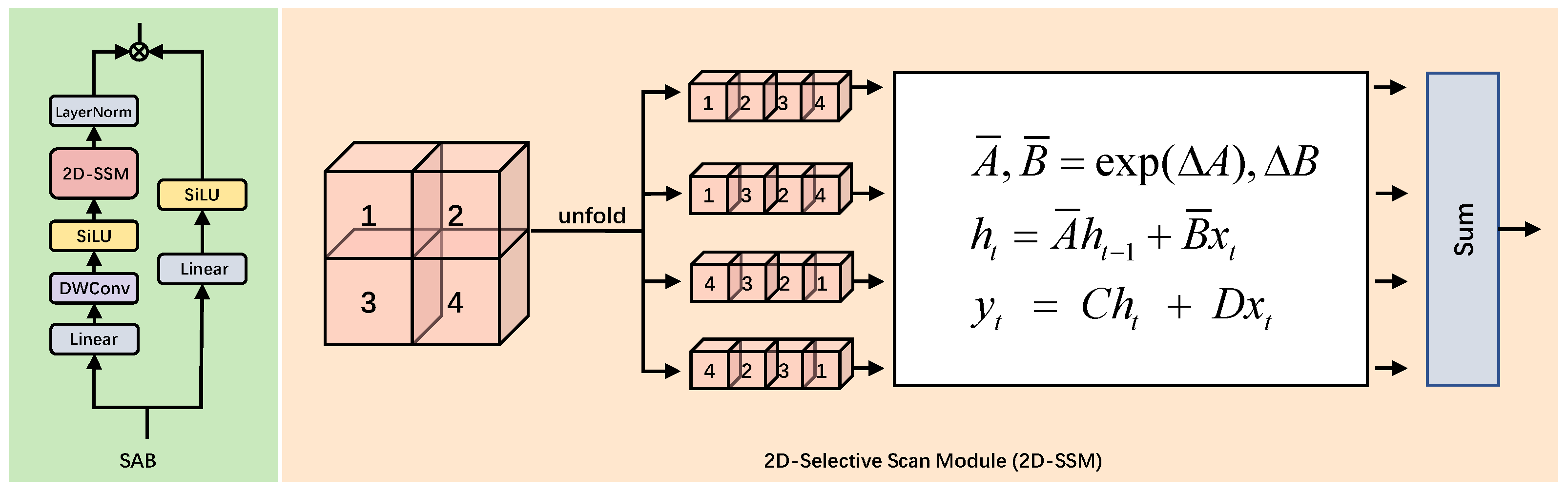
The Spatial Attention Block (SAB) is designed to enhance the modeling of long-range spatial dependencies in 2D image data. As shown in Figure 2, the SAB consists of two main components: the processing path and the 2D Selective Scan Module (2D-SSM).

In the first branch, assuming the input feature has been processed to the feature $F_{\mathrm{in}}\in {\mathbb{R}}^{H\times W\times C}$, it undergoes several transformations to extract spatial information. First, the input feature $F_{\mathrm{in}}$ is processed by a linear layer to reduce its dimensionality and enhance the representation of key features. Then, it passes through a depthwise convolution (DWConv) layer, which captures fine-grained spatial details by applying a filter to each input channel. The convolution result is followed by the SiLU activation function to introduce non-linearity, which helps capture complex relationships within the spatial domain. After SiLU activation, the feature is fed into the 2D-SSM module. The 2D-SSM unfolds the 2D feature map in multiple directions and effectively captures long-range dependencies. Finally, after passing through the 2D-SSM, LayerNorm is applied to stabilize training and maintain consistency across the feature map, producing output $F_1$:

$$F_1=\mathrm{LayerNorm}\left(\text{2D-SSM}\left(\mathrm{SiLU}\left(\mathrm{DWConv}\left(\mathrm{Linear}\left(F_{\mathrm{in}}\right)\right)\right)\right)\right).$$

(11)

In the second branch, the input feature $F_{\mathrm{in}}$ is processed in a simplified manner. First, the feature is mapped to a new feature space by a linear layer, followed by SiLU activation, producing the output $F_2$:

$$F_2=\mathrm{SiLU}\left(\mathrm{Linear}\left(F_{\mathrm{in}}\right)\right).$$

(12)

Then, the outputs from both branches, $F_1$ and $F_2$, are combined using the Hadamard product (element-wise multiplication):

$$F_{\mathrm{out}}=F_1\odot F_2.$$

(13)

This fusion enables the model to integrate spatial information captured by the 2D-SSM in the first branch with the simpler linear feature representation from the second branch, producing the final output via element-wise multiplication.

The 2D-Selective Scan Module (2D-SSM) is the core part of the SAB, as illustrated on the right side of Figure 2. This module unfolds the 2D feature map in four different directions, scanning the image along both the horizontal and vertical axes to capture dependencies between neighboring pixels. This unfolding process effectively captures the long-range spatial dependencies critical to image processing tasks.

After scanning in multiple directions, the results are aggregated and reshaped to reconstruct the original 2D structure of the feature map. This mechanism enables the model to account for both local and global interactions across the image, enhancing its effectiveness in processing complex spatial relationships.

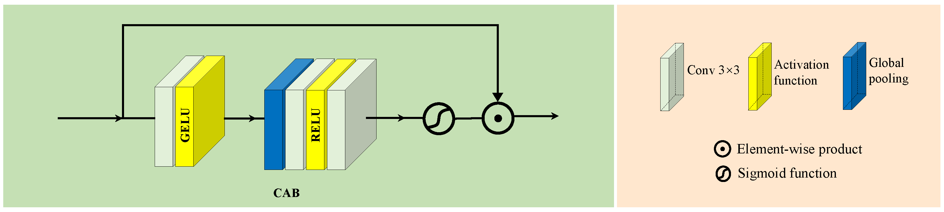
3.4. Channel Attention Block

The Channel Attention Block (CAB) is specifically designed to capture dependencies among different channels in HSIs. In Section 3.3, the SAB focuses on extracting spatial features; however, the spectral dimension has not been sufficiently addressed. Therefore, we introduce the CAB to complement this and explicitly address channel information.

As illustrated in Figure 3, the processing flow of the CAB module is as follows.

First, the input feature map is processed through a convolutional layer to capture initial channel dependencies. The output from this convolutional layer is then processed through the GELU activation function. GELU introduces non-linearity through a probabilistic approach, facilitating the more precise capture of complex channel-wise features.

Next, the features undergo global pooling, which aggregates information across all spatial locations, generating a comprehensive global descriptor for each channel. This step removes the influence of spatial positioning from the channel attention mechanism.

The globally pooled features are then processed through an additional series of convolutional layers to further refine channel dependencies. Afterward, the feature map is once again processed through the RELU activation function for non-linear transformation. Subsequently, the features pass through one final convolutional layer before being fed into a Sigmoid function for normalization. The Sigmoid function constrains the output to the range [0, 1], representing the relative importance of each channel.

Finally, the CAB module applies element-wise multiplication between the channel-wise weights and the input features, amplifying significant channel information while suppressing less relevant channels. This dynamic weighting enables the CAB to effectively enhance the spectral dimension representation within the feature map.

3.5. Loss Function

In our method, we utilize the Mean Relative Absolute Error (MRAE) as the objective function to measure the difference between the predicted and actual HSI cubes. The MRAE loss function is commonly used in HSI reconstruction tasks since it provides a relative measure of the reconstruction error.

Formally, the MRAE loss between the ground-truth HSI $\mathbf{Y}\in {\mathbb{R}}^{H\times W\times N_{\lambda }}$ and the predicted HSI $\widehat{\mathbf{Y}}\in {\mathbb{R}}^{H\times W\times N_{\lambda }}$ is defined as

$$\mathrm{MRAE}(\mathbf{Y},\widehat{\mathbf{Y}})={\displaystyle \frac{1}{N}}\sum _{i=1}^N{\displaystyle \frac{|\mathbf{Y}\left[i\right]-\widehat{\mathbf{Y}}\left[i\right]|}{\mathbf{Y}\left[i\right]}},$$

(14)

where $N=H\times W\times N_{\lambda }$ represents the total number of pixels across all spectral channels in the HSI. Here, H and W denote the height and width of the image, while $N_{\lambda }$ represents the number of spectral bands. The MRAE loss function provides a normalized measurement of the absolute difference between the predicted pixel value $\widehat{\mathbf{Y}}\left[i\right]$ and the ground-truth pixel value $\mathbf{Y}\left[i\right]$, relative to the true pixel value. This formulation ensures that the loss function is scale-invariant and effectively captures the reconstruction error in HSI tasks.

By minimizing the MRAE loss, the model is trained to produce high-quality reconstructed HSIs that are as close as possible to the ground-truth data.

4. Experiments and Analysis

4.1. Dataset Preparation

In this study, we utilized four datasets in total. Three publicly available benchmark datasets were used as the basis for constructing the simulation datasets [44,45,46]. Additionally, a fourth dataset, which was collected from a real-world environment, was used for the experiments in real-world conditions. The details of the three benchmark datasets will be described in Section 4.1, while the description of the fourth dataset will be provided in Section 4.4.4.

4.1.1. Benchmark Datasets

(a)

Chikusei dataset [44]: The Chikusei dataset comprises Hyperspectral Imagery of urban and agricultural regions within the Chikusei area of Ibaraki Prefecture, Japan. The dataset contains 128 spectral bands spanning wavelengths from 363 nm to 1018 nm. Each image has a high spatial resolution of 2048 × 2048 pixels, rendering it a valuable resource for analyzing various landscapes, including urban infrastructure, agricultural fields, forests, and roads. This variety enhances its suitability for a wide range of remote sensing tasks.

(b)

Houston2018 dataset [45]: The Houston2018 dataset contains hyperspectral urban imagery obtained over the University of Houston campus and the surrounding cityscape. The data were collected using the ITRES CASI-1500 hyperspectral sensor, capturing 48 spectral bands over a wavelength range of 380 nm to 1050 nm. Each image has a spatial resolution of 1 m per pixel, with the dimensions being 4172 × 1202 pixels. This dataset is particularly useful for urban scene analysis, given its detailed capture of the urban environment.

(c)

Pavia Centre dataset [46]: Acquired using the Reflective Optics System Imaging Spectrometer, the Pavia Centre dataset contains HSIs taken over the central urban area of Pavia, Italy. The data consist of 102 spectral bands in the 430 nm to 860 nm wavelength range, with noisy bands removed. Each image has a spatial resolution of 1.3 m per pixel and a dimension of 1096 × 1096 pixels. This dataset is commonly used for studying urban features and landscape classification.

4.1.2. Datasets Preprocessing

For ease of performance comparison, we adopted the data preprocessing methods from [34,47,48]. The detailed preprocessing steps for each dataset are outlined below.

(a)

Chikusei dataset: Due to the irrelevance of information in edge areas, we cropped the center region of the original scenes, resulting in an area of 2304 × 2048 × 128. The top section of the cropped images was further segmented into 16 nonoverlapping HSIs of 128 × 128 × 128 each, which were used as the test set. The remainder of the image was cropped into overlapping patches for training purposes, using patches of size 128 × 128 × 128 with an overlap of 64 pixels. We randomly selected 10% of the patches as the validation set.

(b)

Houston2018 dataset: For testing, we cropped the top area of the original image into 16 nonoverlapping HSIs of 128 × 128 × 48. The remainder of the image was then divided into overlapping patches for training, using patches of size 128 × 128 × 48 with a 64-pixel overlap. As with the Chikusei dataset, 10% of the training patches were randomly selected for validation.

(c)

Pavia Centre dataset: The informative region of the original scene was cropped to 1096 × 715 × 102. The left side of the image was segmented into 16 nonoverlapping HSIs of 128 × 128 × 102 for testing. The remaining portion of the image was divided into overlapping training patches of size 128 × 128 × 102 with a 64-pixel overlap. We also randomly selected 10% of the training data as a validation set.

4.1.3. Strong Light Interference Datasets

In this study, we constructed a synthetic hyperspectral dataset with SLI through the following steps, as shown in Figure 4.

(a)

Original HSI: First, we obtained the original HSIs from the benchmark datasets, as shown in Figure 4a. Each HSI consists of multiple channels, where each channel records spectral information at different wavelengths. These channels provide high spectral resolution data and serve as the foundation for constructing the interfered dataset.

(b)

Select Overlay Spot: To simulate real-world SLI, interference spots of varying intensities were collected in a controlled laboratory environment. As illustrated in Figure 4b, the interference spots differ in intensity and shape, and they are randomly applied to different channels of the HSIs. This process simulates the random nature of SLI across different spectral channels. Specifically, the three interference spots used in our experiments had entrance pupil power densities of approximately $6\times {10}^{-7}{\mathrm{W}/\mathrm{cm}}^2$, $2\times {10}^{-6}{\mathrm{W}/\mathrm{cm}}^2$, and $7\times {10}^{-6}{\mathrm{W}/\mathrm{cm}}^2$, respectively.

(c)

Obtain the channel interference intensity of the spot: To precisely simulate the interference intensity on each channel, we established a model based on the spectral characteristics of the light source and the quantum efficiency of the detector. Taking sunlight as an example, the “Spectral curve of light” (shown in Figure 4c) represents the standard solar spectrum, describing the intensity distribution across different wavelengths. The light intensity at each wavelength affects certain channels of the HSI more than others. Additionally, the “Quantum efficiency of detector” curve reflects the detector’s sensitivity at different wavelengths. By multiplying these two curves, we obtain the channel-specific interference intensity, referred to as the “Intensity variation of channels for superposition”, as shown in Figure 4c. If using a different light source, we only need to replace the spectral response curve of the light. This ensures that the intensity variation across channels accurately simulates how different light sources interfere with the HSI.

(d)

Interfered-With HSI: Finally, the adjusted interference spots, based on the calculated intensity variations, are added to the corresponding channels of the original HSI, as shown in Figure 4d. The result is an interfered-with HSI that includes the effects of SLI, simulating real-world conditions of light pollution and interference.

4.2. Implementation Details

In our proposed network, the number of channels in the SSAG module is set to 180, and the number of SSAG modules N is set to 3. The model is trained using the Adam optimizer with parameters ${\beta }_1=0.9$ and ${\beta }_2=0.99$ for 100 epochs. The initial learning rate is set to $5\times {10}^{-5}$, and it decays by a factor of 10 every 150 epochs. The proposed model is implemented using PyTorch 2.1.0 and runs on an NVIDIA RTX 4090 GPU.

4.3. Evaluation Metrics

To thoroughly evaluate the performance of the reconstructed HSIs, we utilize six commonly applied evaluation metrics that account for both spatial and spectral dimensions. The definitions of these metrics are as follows:

MPSNR (Mean Peak Signal-to-Noise Ratio): MPSNR measures the ratio between the maximum possible power of a signal and the power of corrupting noise, averaged across all spectral bands. It is defined as follows:

$$MPSNR={\displaystyle \frac{1}{L}}\sum _{l=1}^{L}10{log}_{10}\left({\displaystyle \frac{MA{X}_l^2}{MS{E}_l}}\right),$$

(15)

where the mean squared error $MS{E}_l$ is given by:

$$MS{E}_l={\displaystyle \frac{1}{WH}}\sum _{w=1}^W\sum _{h=1}^H{\left(I_{rec}(w,h,l)-I_{ori}(w,h,l)\right)}^2,$$

(16)

where L is the total number of spectral bands, W and H denote the width and height of the image, $MA{X}_l$ represents the maximum pixel value within the l-th band, and $I_{rec}$ and $I_{ori}$ denote the reconstructed and original images, respectively.

MSSIM (Mean Structural Similarity Index) [49]: MSSIM evaluates the perceptual similarity between the reconstructed and original images in terms of luminance, contrast, and structure. It is defined as follows:

$$MSSIM={\displaystyle \frac{1}{L}}\sum _{l=1}^L\left({\displaystyle \frac{(2{\mu }_{I_{rec}^l}{\mu }_{I_{ori}^l}+c_1)(2{\sigma }_{I_{rec}^l{I}_{ori}^l}+c_2)}{({\mu }_{I_{rec}^l}^2+{\mu }_{I_{ori}^l}^2+c_1)({\sigma }_{I_{rec}^l}^2+{\sigma }_{I_{ori}^l}^2+c_2)}}\right),$$

(17)

where $\mu$ and $\sigma$ represent the mean and standard deviation, respectively, and $c_1$ and $c_2$ are constants to stabilize the division.

SAM (Spectral Angle Mapper) [50]: SAM measures the spectral similarity between the predicted and original HSIs by calculating the angle between spectral vectors. It is defined as follows:

$$SAM=arccos\left({\displaystyle \frac{\langle I_{rec}^l,I_{ori}^l\rangle }{\parallel I_{rec}^l{\parallel }_2{\parallel I_{ori}^l\parallel }_2}}\right).$$

(18)

CC (Cross-Correlation) [51]: CC quantifies the linear correlation between the reconstructed and original images. It is defined as follows:

$$CC={\displaystyle \frac{1}{L}}\sum _{l=1}^L{\displaystyle \frac{\mathrm{cov}(I_{rec}^l,I_{ori}^l)}{{\sigma }_{I_{rec}^l}{\sigma }_{I_{ori}^l}}}.$$

(19)

RMSE (Root Mean Squared Error): RMSE calculates the standard deviation of the residuals between the predicted and original images. It is defined as follows:

$$RMSE=\sqrt{{\displaystyle \frac{1}{L}}\sum _{l=1}^L{\displaystyle \frac{1}{WH}}\sum _{w=1}^W\sum _{h=1}^H{\left(I_{rec}(w,h,l)-I_{ori}(w,h,l)\right)}^2}.$$

(20)

ERGAS (Erreur Relative Globale Adimensionnelle de Synthèse) [52]: ERGAS is a dimensionless global relative error that evaluates the quality of the reconstructed HSI. It is defined as follows:

$$ERGAS=100s\sqrt{{\displaystyle \frac{1}{L}}\sum _{l=1}^L{\left({\displaystyle \frac{RMS{E}_l}{\mathrm{mean}\left(I_{ori}^l\right)}}\right)}^2},$$

(21)

where s is the scale factor reflecting the sensor’s spatial resolution.

4.4. Comparison with State-of-the-Art Methods

4.4.1. Experiments on the Chikusei Datasets

The experimental results for the Chikusei dataset are shown in

Table 1. Quantitative evaluation of different reconstruction methods on the Chikusei dataset. The best and second-best results are bolded and underlined, respectively.

Method	Params (M)	FLOPs (G)	MPSNR ↑	MSSIM ↑	CC ↑	SAM ↓	RMSE ↓	ERGAS ↓
SERT [30]	1.56	24.67	53.9924	0.9962	0.9943	0.4979	0.0028	1.3519
HSCNN+ [33]	79.02	4.82	52.6159	0.9956	0.9936	0.9124	0.0028	1.7265
MSDformer [34]	123.72	2.15	54.9264	0.9968	0.9960	0.5798	0.0025	1.1684
HAT [53]	285.9	17.53	56.8888	0.9973	0.9972	0.4742	0.0021	0.9659
MambaIR [54]	55.24	4.52	57.5359	0.9964	0.9934	0.7750	0.0018	1.0333
MST++ [36]	97.82	27.06	57.0551	0.9975	0.9972	0.4388	0.0020	0.9612
Ours	130.18	40.18	57.5792	0.9975	0.9973	0.4392	0.0019	0.9172

, where the best results are highlighted in bold and the second-best results are underlined. The arrows in the table indicate performance trends: ↑ indicates better performance as the value increases, while ↓ indicates better performance as the value decreases.

SERT [30] is a hyperspectral denoising method that uses Transformers to enhance spatial and spectral features, achieving superior noise removal performance. HSCNN+ [33] is an early hyperspectral reconstruction method, primarily reconstructing from RGB images, with relatively average overall performance. MSDformer [34] employs a grouping strategy and uses a Transformer to capture long-range dependencies of spectral information, but it still lacks in recovering local spatial details. HAT [53], designed for RGB image restoration with attention to spatial and spectral information, shows potential but may benefit from further adaptation to handle the complexities of hyperspectral data. MambaIR [54], a SOTA model in the Mamba framework for RGB image restoration, struggles with the interference complexities of hyperspectral data. MST++ [36] is the current SOTA model for reconstructing HSIs from RGB images, but it struggles to learn key features in laser interference scenarios, resulting in suboptimal reconstruction performance. Our proposed MambaHR model, through effectively integrating both global and local spatial–spectral information, excels in laser interference scenarios and better handles the effects of complex light spots. The table also presents the parameter counts (Params, M) and floating-point operations (FLOPs, G) for each model, offering insights into their computational complexity. Compared to the CNN-based model HSCNN+, MambaHR exhibits a markedly enhanced ability to capture complex spectral features. In contrast to the Transformer-based model HAT, MambaHR strikes a more favorable balance between computational complexity and reconstruction accuracy. Furthermore, across all the models evaluated, MambaHR consistently achieves the highest performance in key metrics, underscoring its overall superiority in reconstruction tasks.

Figure 5 shows the visualized HSI reconstructions on the Chikusei test set. We selected channels 31, 98, and 61 for RGB visualization to enhance the visual effect and understanding. In scenarios with SLI, we focus specifically on the reconstruction of the peripheral regions of the light spots, as these areas are critical in the test images. The center of the light spot is frequently disrupted by strong light interference, making accurate reconstruction challenging. Thus, the reconstruction accuracy and detail recovery in the non-central regions are particularly significant. It is evident that, while other methods demonstrate some recovery in the edges and details of the light spots, MambaHR excels in these regions, delivering clearer and more precise image details. In particular, the zoomed-in view, highlighted by the red box, emphasizes MambaHR’s advantages in handling complex scenes.

To further assess model performance, we generated difference maps between the reconstructed results and the ground truth (GT), as shown in Figure 6. The difference maps utilize a color scale ranging from blue to red to represent the magnitude of reconstruction errors, with red indicating larger errors and blue indicating smaller errors. The results demonstrate that MambaHR exhibits significantly lower reconstruction errors compared to other methods, highlighting its superior accuracy in scenarios involving complex light interference.

4.4.2. Experiments on the Houston Datasets

The Chikusei dataset is characterized by its grasslands, in stark contrast to the Houston dataset, which boasts a rich array of trees and asphalt roads. This diversity provides a robust test for evaluating our model’s performance across various surface textures and materials. In both qualitative (

Table 2. Quantitative evaluation of different reconstruction methods on the Houston dataset. The best and second-best results are bolded and underlined, respectively.

Method	Params (M)	FLOPs (G)	MPSNR ↑	MSSIM ↑	CC ↑	SAM ↓	RMSE ↓	ERGAS ↓
SERT [30]	1.47	23.25	50.9762	0.9946	0.9883	0.9407	0.0036	1.3292
HSCNN+ [33]	76.84	4.69	53.9585	0.9976	0.9956	0.7986	0.0022	0.9587
MSDformer [34]	54.98	1.56	54.7113	0.9972	0.9958	0.7219	0.0022	0.8246
HAT [53]	283.03	17.36	53.6855	0.9977	0.9962	0.9710	0.0024	1.0784
MambaIR [54]	7.47	0.71	55.8957	0.9736	0.9905	0.9252	0.0047	1.0993
MST++ [36]	14.03	3.86	55.1591	0.9975	0.9951	0.8085	0.0020	0.8416
Ours	18.69	6.08	56.5103	0.9983	0.9973	0.7001	0.0017	0.7358

) and quantitative (Figure 7 and Figure 8) assessments, our MambaHR model demonstrates outstanding performance, showcasing its potent capability in HSI reconstruction tasks within heterogeneous environments.

4.4.3. Experiments on the Pavia Datasets

The Pavia dataset is predominantly composed of urban scenes, featuring a complex mix of buildings and infrastructural elements. This complexity poses significant challenges for the reconstruction of fine spatial structures. On this dataset, our approach consistently outperforms other methods in both qualitative (

Table 3. Quantitative evaluation of different reconstruction methods on the Pavia dataset. The best and second-best results are bolded and underlined, respectively.

Method	Params (M)	FLOPs (G)	MPSNR ↑	MSSIM ↑	CC ↑	SAM ↓	RMSE ↓	ERGAS ↓
SERT [30]	1.53	24.21	36.2808	0.9695	0.9706	2.3317	0.0172	3.0529
HSCNN+ [33]	78.31	4.78	38.0524	0.9753	0.9790	2.7667	0.0138	2.5925
MSDformer [34]	102.54	1.96	39.2865	0.9785	0.9836	2.4444	0.0124	2.2404
HAT [53]	284.97	17.48	40.9026	0.9861	0.9898	2.1132	0.0103	1.8156
MambaIR [54]	54.5	4.48	41.2786	0.9853	0.9862	2.1271	0.0115	1.8490
MST++ [36]	62.31	17.22	41.0852	0.9845	0.9891	1.8473	0.0103	1.7910
Ours	83.04	25.85	41.3219	0.9864	0.9901	1.7913	0.0100	1.7329

) and quantitative (Figure 9 and Figure 10) comparisons, proving how effectively the MambaHR model can distinguish between different urban features, such as buildings and roads, thus highlighting its exceptional ability to reconstruct intricate spatial structures.

4.4.4. Experiments on the Real-World Scenarios

In this experiment, we utilized an xiSpec2 hyperspectral camera equipped with the CMV2K-LS-150-470-900 chip to capture images of a custom-made target. Various intensities of light interference were applied during the capture process, with the collected wavelengths ranging from 460 nm to 890 nm.

Figure 11 illustrates the spatial restoration results under six different levels of light interference. The hyperspectral data are visualized using spectral bands 28, 64, and 116 as R, G, and B, respectively. It is evident that our model successfully restores the general outline information in the spatial domain; however, further improvements are needed for finer details, particularly when interference intensity is high and affects larger areas. As the interference intensity increases, the quality of the spatial restoration degrades, especially in regions where the interference spans a broader area.

Figure 12 presents the spectral curves for the cases of interfered3, interfered5, and interfered6, corresponding to subplots (a), (b), and (c) in Figure 11. These curves are derived from pixel points highlighted by red boxes in Figure 11. We selected pixels around the interference center, as the central regions of strong light interference typically suffer from a near-total loss of spatial and spectral information. Hence, we consider that accurate restoration at the very center of interference is challenging. In contrast, areas surrounding the interference center, which retain partial spatial and spectral information, offer a higher potential for restoration. As shown in Figure 12, the spectral curves in the interference regions are significantly degraded, with damage increasing alongside the intensity of light interference from (a) to (c). Despite this, our method demonstrates a strong capability for restoring the spectral dimension, bringing the reconstructed curves closer to the original spectral values. While the restoration of spatial texture details remains limited, the spectral restoration is sufficiently accurate for recognition and subsequent analysis tasks.

5. Ablation Study

The effectiveness of the spatial and Channel Attention Block: We conducted ablation experiments to assess the impact of the SAB and the CAB in the proposed model across the Chikusei, Houston, and Pavia datasets. As shown in

Table 4. Ablation experiments of some variants of the proposed method on the Chikusei testing dataset. Bold represents the best results.

Variant	Params. ($\times {10}^6$)	PSNR ↑	SSIM ↑	CC ↑	SAM ↓	RMSE ↓	ERGAS ↓
w/o SAB	29.6028	56.9449	0.9719	0.9906	0.9580	0.0053	1.9493
w/o CAB	32.4538	57.5328	0.9969	0.9763	0.3838	0.0022	1.0856
MambaHR	40.1843	57.5792	0.9976	0.9973	0.4392	0.0019	0.9172

,

Table 5. Ablation experiments of some variants of the proposed method on the Houston testing dataset. Bold represents the best results.

Variant	Params. ($\times {10}^6$)	PSNR ↑	SSIM ↑	CC ↑	SAM ↓	RMSE ↓	ERGAS ↓
w/o SAB	4.205754	56.2526	0.9990	0.9883	1.1269	0.0007	1.1417
w/o CAB	4.981680	56.0304	0.9929	0.9800	1.1572	0.0021	1.5352
MambaHR	6.077178	56.5103	0.9983	0.9973	0.7001	0.0017	0.7358

and

Table 6. Ablation experiments of some variants of the proposed method on the Pavia testing dataset. Bold represents the best results.

Variant	Params. ($\times {10}^6$)	PSNR ↑	SSIM ↑	CC ↑	SAM ↓	RMSE ↓	ERGAS ↓
w/o SAB	18.84511	41.3934	0.9759	0.9714	2.69497	0.0133	1.8366
w/o CAB	20.91854	41.2255	0.9517	0.9686	1.8739	0.0124	2.0192
MambaHR	25.85046	41.3219	0.9864	0.9901	1.7913	0.0100	1.7329

, the removal of SAB (denoted as “w/o SAB”) led to an overall decline in model performance, although the extent of the impact varied across different datasets. Similarly, removing CAB (denoted as “w/o CAB”) also resulted in a general performance drop. These results confirm that both SAB and CAB play a crucial role in effectively extracting spatial and spectral information, contributing to a comprehensive understanding of HSIs.

The effectiveness of deformable convolution: To further examine the influence of the number of SSAGs, we varied the number from $N=2$ to $N=5$, as shown in

Table 7. Quantitative comparisons of the number of SSAGs on the Chikusei testing dataset. Bold represents the best results.

Variant	Params. ($\times {10}^6$)	PSNR ↑	SSIM ↑	SAM ↓	CC ↑	RMSE ↓	ERGAS ↓
N = 2	26.8878	57.1880	0.9872	0.5749	0.9715	0.0042	1.7612
N = 3	40.1843	57.5792	0.9975	0.4392	0.9973	0.0020	0.9172
N = 4	53.4808	57.5160	0.9962	0.4070	0.9883	0.0024	1.0928
N = 5	66.7772	57.3518	0.9940	0.4145	0.9864	0.0036	1.4098

. When $N=3$ was used, the model achieved the best overall performance on most metrics. As the number of SSAGs exceeded this value, performance started to decline, likely due to the network becoming too complex for the available training data. Therefore, using $N=3$ SSAGs strikes a balance between model complexity and performance.

6. Conclusions

In this paper, we propose MambaHR, a novel HSI restoration framework specifically designed to address the issue of SLI during imaging. By utilizing a selective SSM combined with channel attention mechanisms, MambaHR effectively integrates both global and local spatial–spectral dependencies, enabling accurate restoration of HSIs while preserving essential spectral and spatial details. We also simulate real-world light interference scenarios by developing a flexible spectral simulation approach that can adapt to various types of light sources. Utilizing this method, we created new datasets derived from benchmark datasets, including Chikusei, Houston, and Pavia. Experimental results demonstrate that MambaHR achieves superior performance in both qualitative and quantitative evaluations, significantly surpassing existing methods. Future research will concentrate on improving the model’s generalization capabilities under more diverse and complex lighting conditions. Additionally, we plan to further optimize the Mamba architecture through hardware programming and focus on improving the restoration of spatial information in real-world scenarios, particularly in challenging environments with significant noise interference.

References

1. Zhang, Q.; Willmott, M.B. Review of Hyperspectral Imaging in Environmental Monitoring Progress and Applications. Acad. J. Sci. Technol. 2023, 6, 9–11. [Google Scholar] [CrossRef]
2. Rajabi, R.; Zehtabian, A.; Singh, K.D.; Tabatabaeenejad, A.; Ghamisi, P.; Homayouni, S. Hyperspectral Imaging in environmental monitoring and analysis. Front. Environ. Sci. 2024, 11, 1353447. [Google Scholar] [CrossRef]
3. Shimoni, M.; Haelterman, R.; Perneel, C. Hypersectral Imaging for Military and Security Applications: Combining Myriad Processing and Sensing Techniques. IEEE Geosci. Remote Sens. Mag. 2019, 7, 101–117. [Google Scholar] [CrossRef]
4. Eismann, M.T.; Stocker, A.D.; Nasrabadi, N.M. Automated hyperspectral cueing for civilian search and rescue. Proc. IEEE 2009, 97, 1031–1055. [Google Scholar] [CrossRef]
5. Bhargava, A.; Sachdeva, A.; Sharma, K.; Alsharif, M.H.; Uthansakul, P.; Uthansakul, M. Hyperspectral Imaging and Its Applications: A Review. Heliyon 2024, 10, e33208. [Google Scholar] [CrossRef]
6. Qu, Y.; Jiang, Y.; He, Y.; Qiu, Z.; Wang, S.; Sun, D. A method of reducing stray light of 1.5 μm laser 3D vision system. Infrared Phys. Technol. 2018, 92, 266–269. [Google Scholar] [CrossRef]
7. Shen, S.; Zhu, J.; Huang, X.; Shen, W. Suppression of the Self-Radiation Stray Light of Long-Wave Thermal Infrared Imaging Spectrometers. In Proceedings of the 5th International Symposium of Space Optical Instruments and Applications, Beijing, China, 5–7 September 2018; Springer: Berlin/Heidelberg, Germany, 2020; pp. 101–110. [Google Scholar]
8. Zhang, X.; Li, B.; Zhi, D.D.; Fang, X.; Li, T.; Du, W.F.; Wang, X.X.; Li, H.S.; Sun, F.K.; Gu, G.C. Stray light analysis and suppression of a UV multiple sub-pupil ultra-spectral imager. Appl. Opt. 2024, 63, 6112–6120. [Google Scholar] [CrossRef]
9. Lu, Y.; Xu, X.; Zhang, N.; Lv, Y.; Xu, L. Study on stray light testing and suppression techniques for large-field of view multispectral space optical systems. IEEE Access 2024, 12, 33938–33948. [Google Scholar] [CrossRef]
10. Lü, B.; Feng, R.; Kou, W.; Liu, W.Q. Optical system design and stray light suppression of catadioptric space camera. Chin. Opt. 2020, 13, 822. [Google Scholar]
11. Li, H.; Yihua, H. Laser Active Jamming of Photo-electric Imaging System and Its Computer Simulation. Laser Optoelectron. Prog. 2006, 43, 39. [Google Scholar]
12. Meng, F.; Xing, Z.; Xu, Z.; Chen, X. Simulation study of strong light interference effect in temporally and spatially modulated Fourier transform imaging spectrometer. High Power Laser Part. Beams 2022, 34, 011010. [Google Scholar]
13. Xu, Y.; Sun, X.; Shao, L. Impact of laser jamming on target detection performance in CCD imaging system. Infrared Laser Eng. 2012, 41, 989–993. [Google Scholar]
14. Cha, J.D.; Lee, J.H.; Kim, S.H.; Jung, D.H.; Kim, Y.S.; Jeong, Y. Through-field Investigation of Stray Light for the Fore-optics of an Airborne Hyperspectral Imager. Curr. Opt. Photonics 2022, 6, 313–322. [Google Scholar]
15. Wang, H.; Chen, Q.; Ma, Z.; Yan, H.; Lin, S.; Xue, Y. Development and Prospect of Stray Light Suppression and Evaluation Technology (Invited). Acta Photonica Sin. 2022, 51, 0751406. [Google Scholar]
16. Donval, A.; Fisher, T.; Lipman, O.; Oron, M. Smart filters: Protect from laser threats. In Proceedings of the Laser Technology for Defense and Security X, Baltimore, MD, USA, 5–9 May 2014; SPIE: Cergy-Pontoise, France, 2014; Volume 9081, pp. 28–34. [Google Scholar]
17. Gralewicz, G.; Owczarek, G. Analysis of the selected optical parameters of filters protecting against hazardous infrared radiation. Int. J. Occup. Saf. Ergon. 2016, 22, 305–309. [Google Scholar] [CrossRef]
18. Matsniev, I.; Andriichuk, V.; Chumak, O.; Derzhypolsky, A.; Derzhypolska, L.; Khodakovskiy, V.; Perederiy, O.; Negriyko, A. The Threshold of Laser-Induced Damage of Image Sensors in Open Atmosphere. In Proceedings of the International Conference on Nanotechnology and Nanomaterials, Palma, Spain, 4–8 July 2022; Springer: Berlin/Heidelberg, Germany, 2022; pp. 299–322. [Google Scholar]
19. Boracchi, G.; Foi, A. Modeling the performance of image restoration from motion blur. IEEE Trans. Image Process. 2012, 21, 3502–3517. [Google Scholar] [CrossRef]
20. Zhang, L.; Zuo, W. Image restoration: From sparse and low-rank priors to deep priors [lecture notes]. IEEE Signal Process. Mag. 2017, 34, 172–179. [Google Scholar] [CrossRef]
21. Jia, S.; Jiang, S.; Lin, Z.; Li, N.; Xu, M.; Yu, S. A survey: Deep learning for Hyperspectral Image classification with few labeled samples. Neurocomputing 2021, 448, 179–204. [Google Scholar] [CrossRef]
22. Wang, X.; Hu, Q.; Cheng, Y.; Ma, J. Hyperspectral Image super-resolution meets deep learning: A survey and perspective. IEEE/CAA J. Autom. Sin. 2023, 10, 1668–1691. [Google Scholar] [CrossRef]
23. Ahmad, M.; Shabbir, S.; Roy, S.K.; Hong, D.; Wu, X.; Yao, J.; Khan, A.M.; Mazzara, M.; Distefano, S.; Chanussot, J. Hyperspectral Image classification—Traditional to deep models: A survey for future prospects. IEEE J. Sel. Top. Appl. Earth Obs. Remote Sens. 2021, 15, 968–999. [Google Scholar] [CrossRef]
24. Vaswani, A.; Shazeer, N.M.; Parmar, N.; Uszkoreit, J.; Jones, L.; Gomez, A.N.; Kaiser, L.; Polosukhin, I. Attention is All you Need. In Proceedings of the Neural Information Processing Systems, Long Beach, CA, USA, 4–9 December 2017. [Google Scholar]
25. Gu, A.; Goel, K.; Ré, C. Efficiently Modeling Long Sequences with Structured State Spaces. In Proceedings of the International Conference on Learning Representations (ICLR), Virtual, 25–29 April 2022. [Google Scholar]
26. Gu, A.; Dao, T. Mamba: Linear-time sequence modeling with selective state spaces. arXiv 2023, arXiv:2312.00752. [Google Scholar]
27. Rasti, B.; Ulfarsson, M.O.; Ghamisi, P. Automatic Hyperspectral Image restoration using sparse and low-rank modeling. IEEE Geosci. Remote Sens. Lett. 2017, 14, 2335–2339. [Google Scholar] [CrossRef]
28. Liu, N.; Li, W.; Wang, Y.; Tao, R.; Du, Q.; Chanussot, J. A survey on Hyperspectral Image restoration: From the view of low-rank tensor approximation. Sci. China Inf. Sci. 2023, 66, 140302. [Google Scholar] [CrossRef]
29. Zhao, B.; Ulfarsson, M.O.; Sigurdsson, J. Hyperspectral Image Denoising Using Low-Rank and Sparse Model Based Deep Unrolling. In Proceedings of the IGARSS 2023—2023 IEEE International Geoscience and Remote Sensing Symposium, Pasadena, CA, USA, 16–21 July 2023; IEEE: Piscataway, NJ, USA, 2023; pp. 5818–5821. [Google Scholar]
30. Li, M.; Liu, J.; Fu, Y.; Zhang, Y.; Dou, D. Spectral Enhanced Rectangle Transformer for Hyperspectral Image Denoising. In Proceedings of the IEEE/CVF Conference on Computer Vision and Pattern Recognition (CVPR), Vancouver, BC, Canada, 18–22 June 2023. [Google Scholar]
31. Maffei, A.; Haut, J.M.; Paoletti, M.E.; Plaza, J.; Bruzzone, L.; Plaza, A. A single model CNN for Hyperspectral Image denoising. IEEE Trans. Geosci. Remote Sens. 2019, 58, 2516–2529. [Google Scholar] [CrossRef]
32. Sidorov, O.; Hardeberg, J.Y. Deep Hyperspectral Prior: Single-Image Denoising, Inpainting, Super-Resolution. In Proceedings of the 2019 IEEE/CVF International Conference on Computer Vision Workshop (ICCVW), Seoul, Republic of Korea, 27–28 October 2019; pp. 3844–3851. [Google Scholar]
33. Shi, Z.; Chen, C.; Xiong, Z.; Liu, D.; Wu, F. Hscnn+: Advanced cnn-based hyperspectral recovery from rgb images. In Proceedings of the IEEE Conference on Computer Vision and Pattern Recognition Workshops, Salt Lake City, UT, USA, 18–22 June 2018; pp. 939–947. [Google Scholar]
34. Chen, S.; Zhang, L.; Zhang, L. MSDformer: Multiscale Deformable Transformer for Hyperspectral Image Super-Resolution. IEEE Trans. Geosci. Remote Sens. 2023, 61, 3315970. [Google Scholar] [CrossRef]
35. Zhang, Q.; Dong, Y.; Zheng, Y.; Yu, H.; Song, M.; Zhang, L.; Yuan, Q. Three-Dimension spatial–spectral Attention Transformer for Hyperspectral Image Denoising. IEEE Trans. Geosci. Remote. Sens. 2024, 62, 3458174. [Google Scholar] [CrossRef]
36. Cai, Y.; Lin, J.; Lin, Z.; Wang, H.; Zhang, Y.; Pfister, H.; Timofte, R.; Van Gool, L. Mst++: Multi-stage spectral-wise transformer for efficient spectral reconstruction. In Proceedings of the IEEE/CVF Conference on Computer Vision and Pattern Recognition, New Orleans, LA, USA, 18–24 June 2022; pp. 745–755. [Google Scholar]
37. Qu, H.; Ning, L.; An, R.; Fan, W.; Derr, T.; Liu, H.; Xu, X.; Li, Q. A survey of mamba. arXiv 2024, arXiv:2408.01129. [Google Scholar]
38. Fu, G.; Xiong, F.; Lu, J.; Zhou, J. Ssumamba: Spatial–spectral selective state space model for Hyperspectral Image denoising. IEEE Trans. Geosci. Remote. Sens. 2024, 62, 1–14. [Google Scholar] [CrossRef]
39. Dong, J.; Yin, H.; Li, H.; Li, W.; Zhang, Y.; Khan, S.; Khan, F.S. Dual Hyperspectral Mamba for Efficient Spectral Compressive Imaging. arXiv 2024, arXiv:2406.00449. [Google Scholar]
40. Chen, M.; Zhao, Y.; Yang, W.; Qian, J.; Li, S.; Zheng, Y.; Ma, J.; Wang, S.; Chen, J.; Wei, J. A model for suppressing stray light in astronomical images based on deep learning. Sci. Rep. 2024, 14, 27521. [Google Scholar] [CrossRef]
41. Zhang, Z.; Xing, Y.; Huang, Y.; Chang, J.; Wu, Z.; Duan, Z.; Song, J. Stray light suppression of opto-mechanical system based on deep reinforcement learning. Optica Open, 19 September 2023. [Google Scholar]
42. Li, Y.; Niu, Z.; Sun, Q.; Xiao, H.; Li, H. BSC-Net: Background Suppression Algorithm for Stray Lights in Star Images. Remote Sens. 2022, 14, 4852. [Google Scholar] [CrossRef]
43. Ziyang, Z.; Jun, C.; Yifan, H.; Qinfang, C.; Yunan, W. Reinforcement learning-based stray light suppression study for space-based gravitational wave detection telescope system. Opto-Electron. Eng. 2024, 51, 230210. [Google Scholar]
44. Yokoya, N.; Iwasaki, A. Airborne hyperspectral Data over Chikusei; Technical Report SAL-2016-05-27; Space Application Laboratory, University of Tokyo: Tokyo, Japan, 2016. [Google Scholar]
45. Xu, Y.; Du, B.; Zhang, L.; Cerra, D.; Pato, M.; Carmona, E.; Prasad, S.; Yokoya, N.; Hänsch, R.; Le Saux, B. Advanced Multi-Sensor Optical Remote Sensing for Urban Land Use and Land Cover Classification: Outcome of the 2018 IEEE GRSS Data Fusion Contest. IEEE J. Sel. Top. Appl. Earth Obs. Remote Sens. 2019, 12, 1709–1724. [Google Scholar] [CrossRef]
46. Huang, X.; Zhang, L. A comparative study of spatial approaches for urban mapping using hyperspectral ROSIS images over Pavia City, northern Italy. Int. J. Remote Sens. 2009, 30, 3205–3221. [Google Scholar] [CrossRef]
47. Jiang, J.; Sun, H.; Liu, X.; Ma, J. Learning spatial–spectral Prior for Super-Resolution of Hyperspectral Imagery. IEEE Trans. Comput. Imaging 2020, 6, 1082–1096. [Google Scholar] [CrossRef]
48. Wang, X.; Ma, J.; Jiang, J. Hyperspectral Image Super-Resolution via Recurrent Feedback Embedding and spatial–spectral Consistency Regularization. IEEE Trans. Geosci. Remote Sens. 2022, 60, 1–13. [Google Scholar] [CrossRef]
49. Wang, Z.; Bovik, A.; Sheikh, H.; Simoncelli, E. Image quality assessment: From error visibility to structural similarity. IEEE Trans. Image Process. 2004, 13, 600–612. [Google Scholar] [CrossRef]
50. Yuhas, R.H.; Goetz, A.F.; Boardman, J.W. Discrimination among semi-arid landscape endmembers using the spectral angle mapper (SAM) algorithm. In Proceedings of the Jet Propulsion Laboratory (JPL), Summaries of the Third Annual JPL Airborne Geoscience Workshop, Pasadena, CA, USA, 1–5 June 1992; Volume 1. [Google Scholar]
51. Loncan, L.; De Almeida, L.B.; Bioucas-Dias, J.M.; Briottet, X.; Chanussot, J.; Dobigeon, N.; Fabre, S.; Liao, W.; Licciardi, G.A.; Simoes, M.; et al. Hyperspectral pansharpening: A review. IEEE Geosci. Remote Sens. Mag. 2015, 3, 27–46. [Google Scholar] [CrossRef]
52. Wald, L. Data Fusion: Definitions and Architectures: Fusion of Images of Different Spatial Resolutions; Presses des MINES: Paris, France, 2002. [Google Scholar]
53. Chen, X.; Wang, X.; Zhou, J.; Qiao, Y.; Dong, C. Activating More Pixels in Image Super-Resolution Transformer. In Proceedings of the IEEE/CVF Conference on Computer Vision and Pattern Recognition (CVPR), Vancouver, BC, Canada, 18–22 June 2023; pp. 22367–22377. [Google Scholar]
54. Guo, H.; Li, J.; Dai, T.; Ouyang, Z.; Ren, X.; Xia, S.T. MambaIR: A Simple Baseline for Image Restoration with State-Space Model. In Proceedings of the European Conference on Computer Vision (ECCV), Milan, Italy, 29 September–4 October 2024. [Google Scholar]
Figure 1. The overall architecture of MambaHR and the structure of the SSAGs and SSABs: (a) the main pipeline of MambaHR operation, wherein the detailed structure of the SSAGs and SSABs is elucidated in (b,c).
Remotesensing 16 04661 g001
Figure 2. The structure of the Spatial Attention Block.
Remotesensing 16 04661 g002
Figure 3. The structure of the Channel Attention Block.
Remotesensing 16 04661 g003
Figure 4. Simulation process of Hyperspectral Image interference with stray light.
Remotesensing 16 04661 g004
Figure 5. Reconstruction in the Chikusei dataset with spectral bands 31-98-61 as R-G-B. From left to right, ground truth, laser interfered image, and results of SERT [30], HSCNN+ [33], MSDformer [34], HAT [53], MambaIR [54], MST++ [36] and the proposed MambaHR method.
Remotesensing 16 04661 g005
Figure 6. Error maps of the test HSIs in the Chikusei dataset, obtained by calculating the difference between the reconstructed results and the GT.
Remotesensing 16 04661 g006
Figure 7. Reconstruction in the Houston dataset with spectral bands 29-26-19 as R-G-B. From left to right, ground truth, laser interfered image, and results of SERT [30], HSCNN+ [33], MSDformer [34], HAT [53], MambaIR [54], MST++ [36] and the proposed MambaHR method.
Remotesensing 16 04661 g007
Figure 8. Error maps of the test HSIs in the Houston dataset, obtained by calculating the difference between the reconstructed results and the GT.
Remotesensing 16 04661 g008
Figure 9. Reconstruction in the Pavia dataset with spectral bands 100-30-12 as R-G-B. From left to right, ground truth, laser interfered image, then results of SERT [30], HSCNN+ [33], MSDformer [34], HAT [53], MambaIR [54], MST++ [36] and the proposed MambaHR method.
Remotesensing 16 04661 g009
Figure 10. Error maps of the test HSIs in the Pavia dataset, obtained by calculating the difference between the reconstructed results and the GT.
Remotesensing 16 04661 g010
Figure 11. Spatial restoration results (with spectral bands 28-64-116 as R-G-B) under different light interference levels and corresponding recovery results.
Remotesensing 16 04661 g011
Figure 12. Spectral restoration results for pixel points in the red boxes from interfered3, interfered5, and interfered6 in Figure 11. Subplots (ac) correspond to interfered3, interfered5, and interfered6, respectively, showing the original, interfered, and restored spectral curves for the selected points.
Remotesensing 16 04661 g012