
Reconstructing Long-Term, High-Resolution Groundwater Storage Changes in the Songhua River Basin Using Supplemented GRACE and GRACE-FO Data


Abstract

1. Introduction
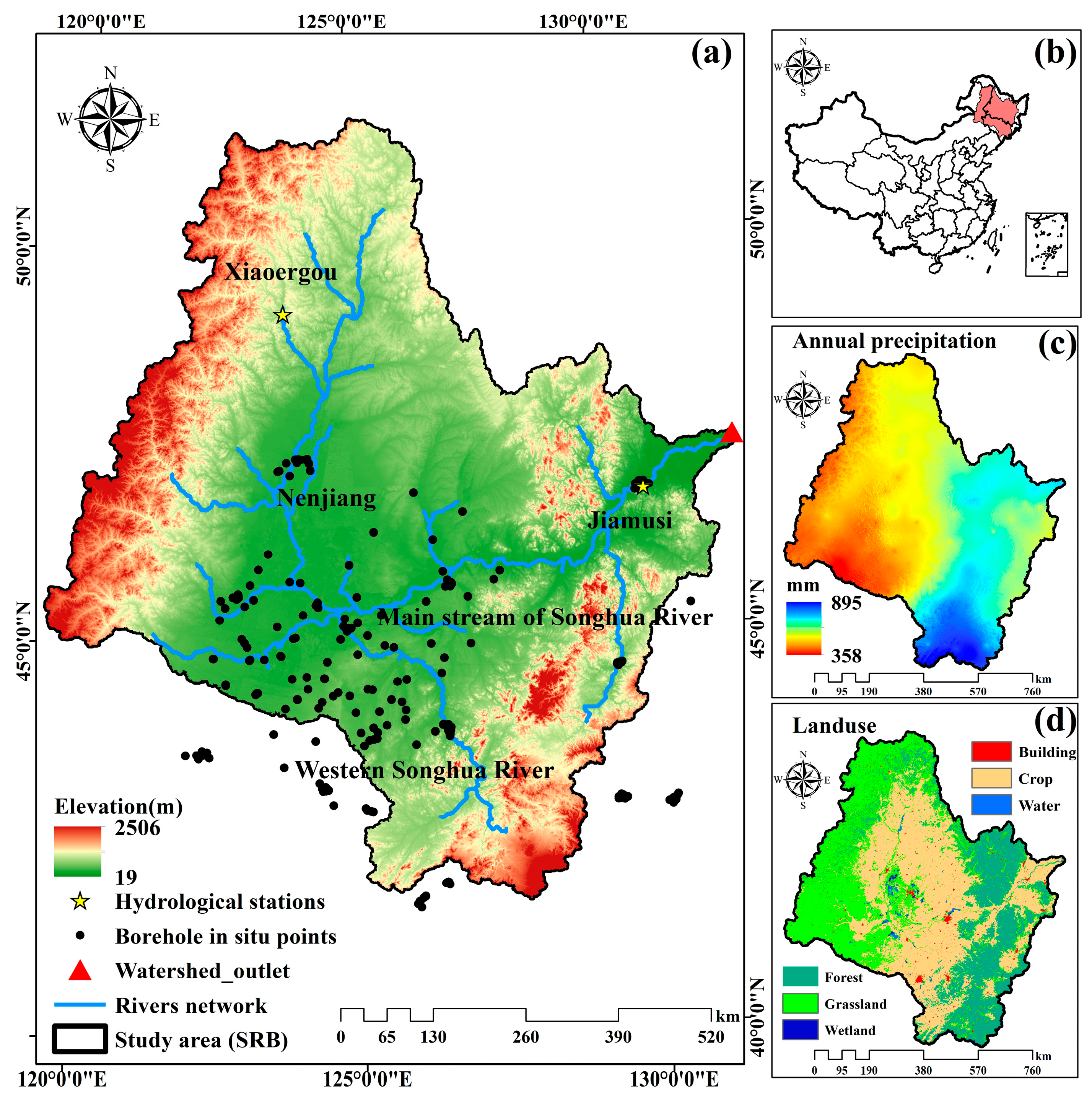
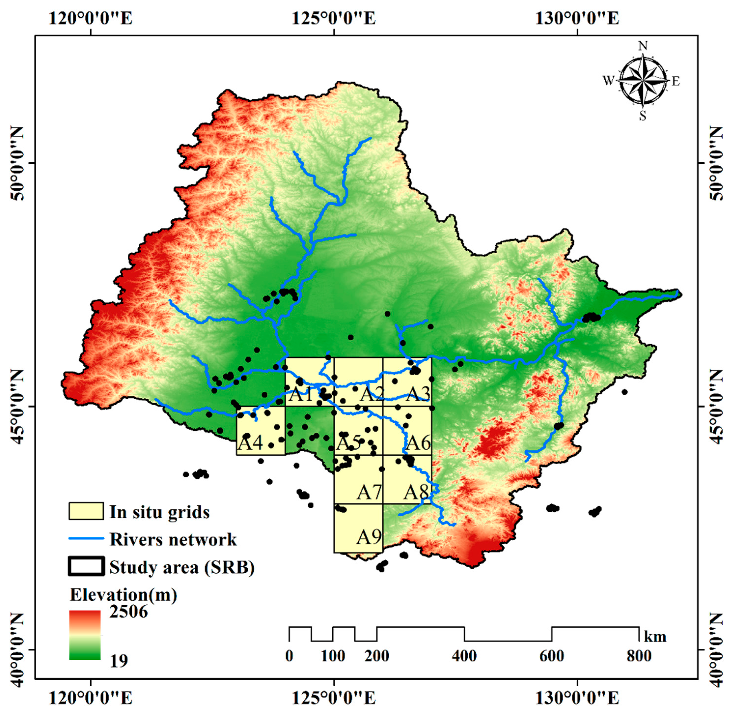
2. Study Area
3. Materials and Methodology
3.1. Input Datasets
3.1.1. GRACE/GRACE-FO Data
3.1.2. GLDAS Model Data
3.1.3. ESSI-3 Model Data
3.1.4. Environmental Variables
3.1.5. Ground-Based Measurements
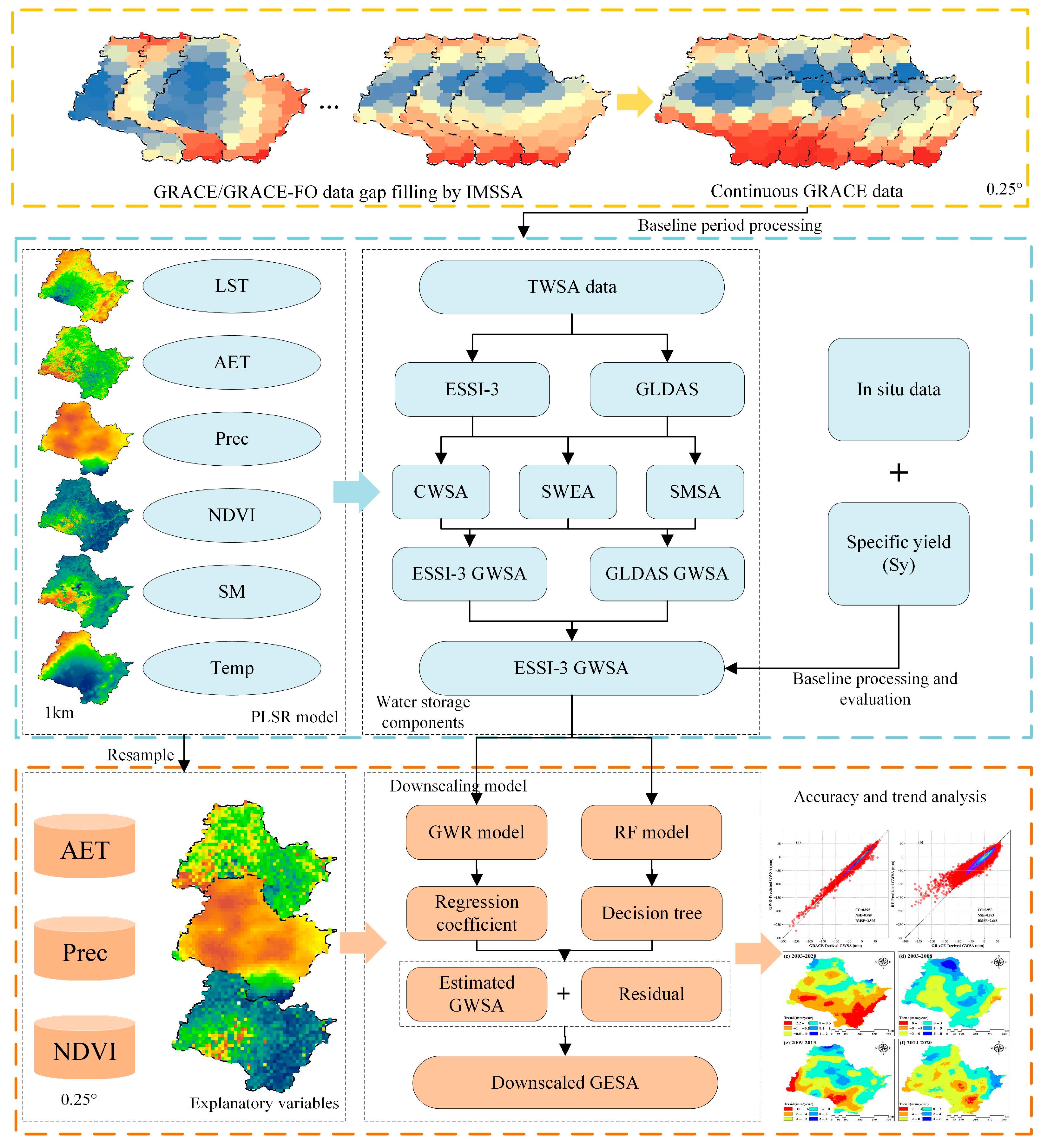
3.2. Methodology
3.2.1. Partial Least Squares Regression
3.2.2. Interpolated Multi-Channel Singular Spectrum Analysis
- (1)
- Constructing the Embedding Matrix
- (2)
- Singular Value Decomposition (SVD)
- (3)
- Time Series Reconstruction
3.2.3. Groundwater Storage Anomaly Estimation
3.2.4. Random Forest Method
3.2.5. Geographically Weighted Regression Model
3.2.6. Hydrological Model ESSI-3
3.2.7. Evaluation Indicators
4. Results
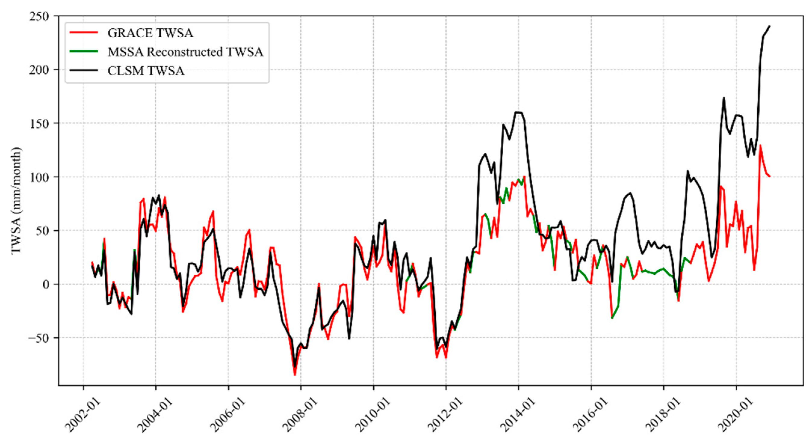
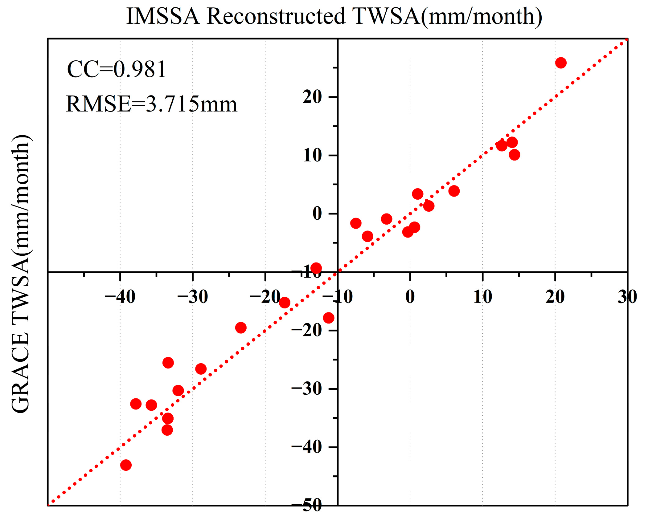
4.1. Reconstruction of Missing GRACE/GRACE-FO Data
4.2. Performance of Hydrological Models and Determination of Water Storage Components
4.3. Selection of Environmental Variables
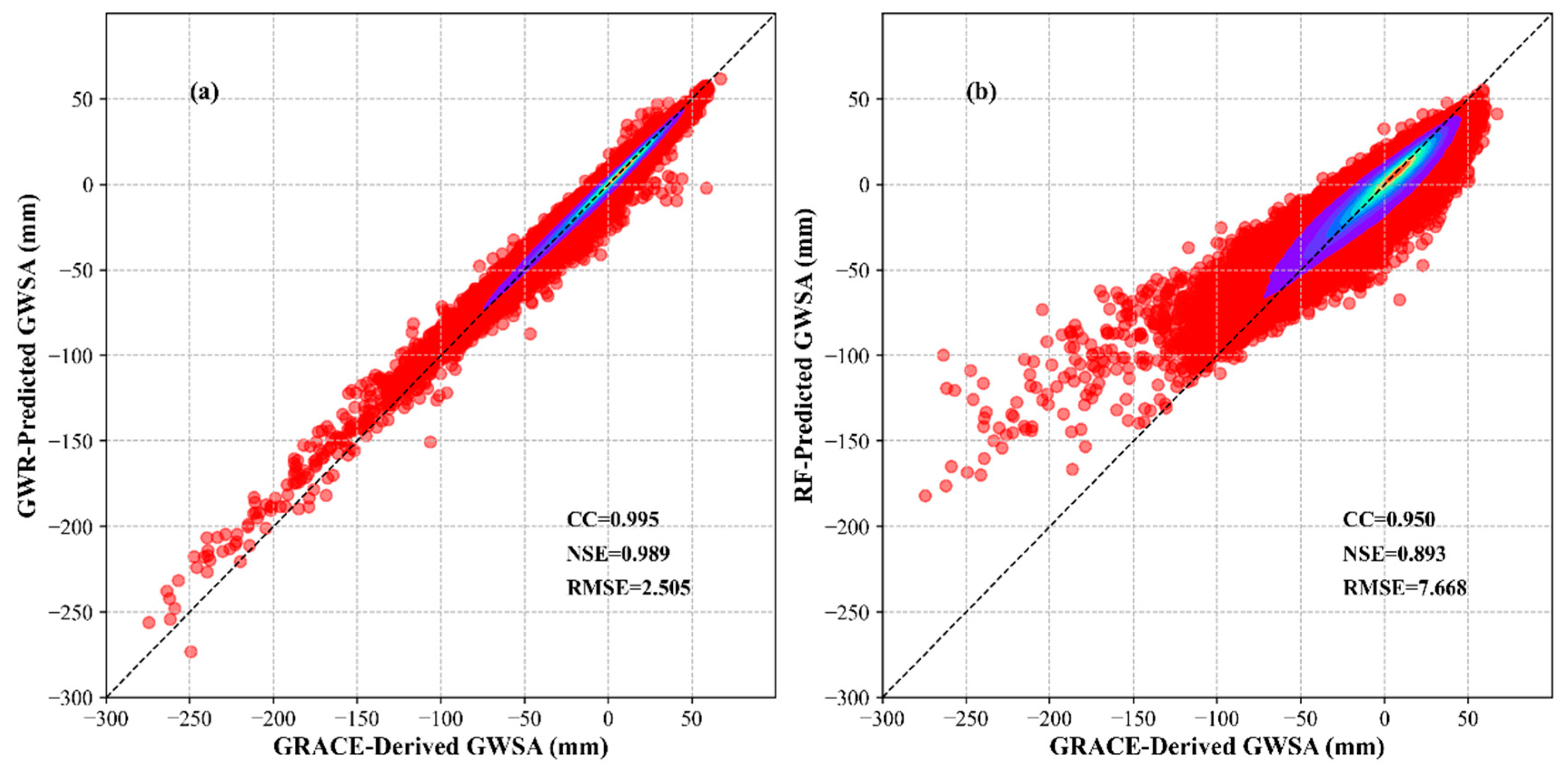
4.4. Comparison of Downscaling Models
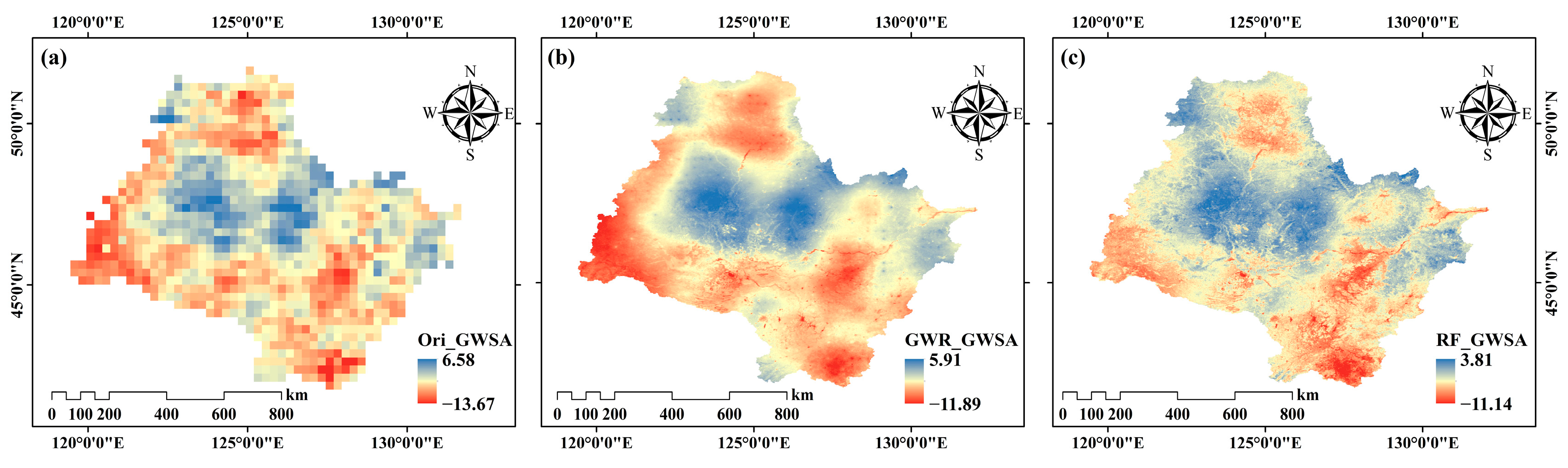
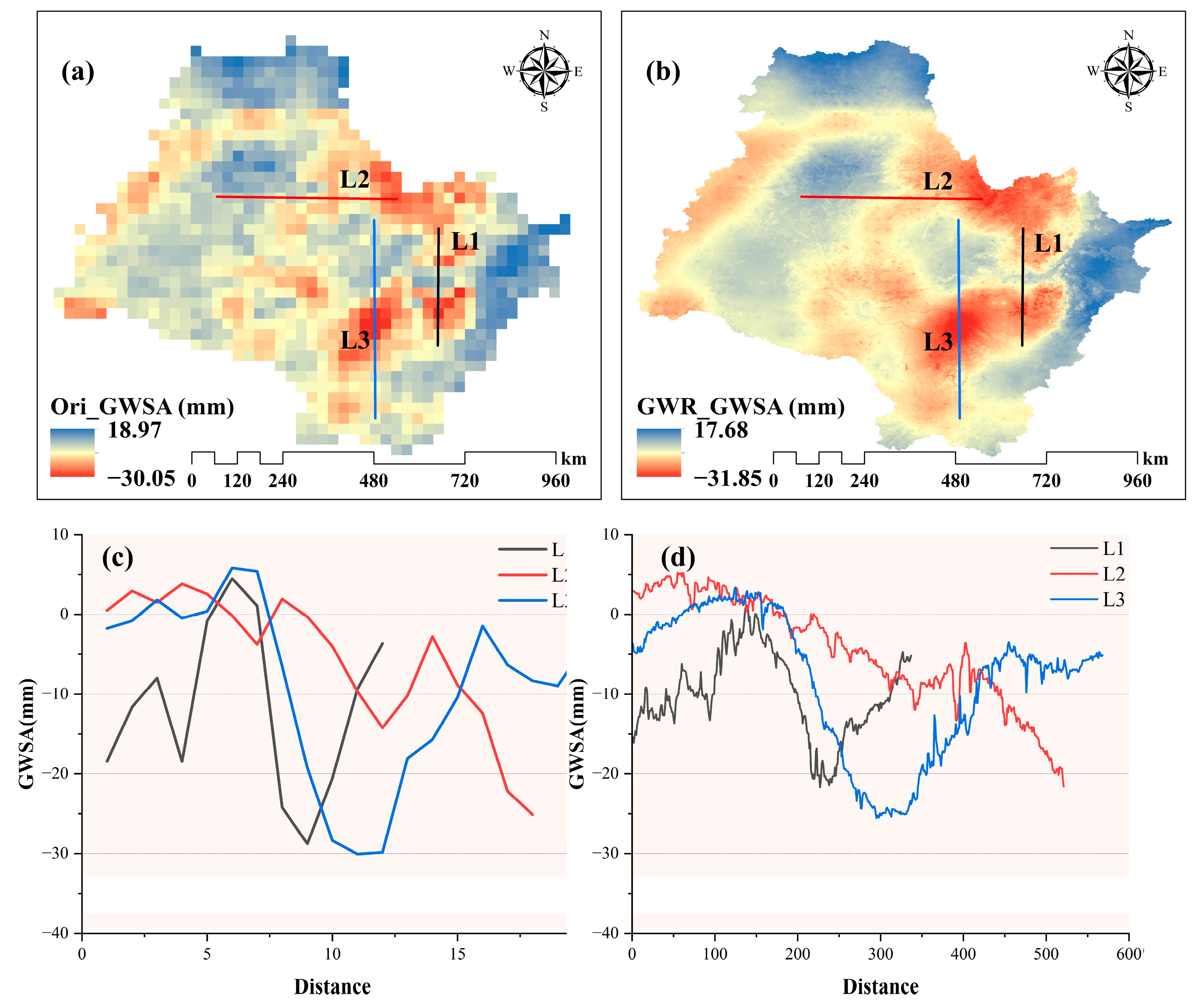
4.5. Analysis of GWSA Downscaling Results
5. Discussion
5.1. Performance of the Proposed Downscaling Model and Method
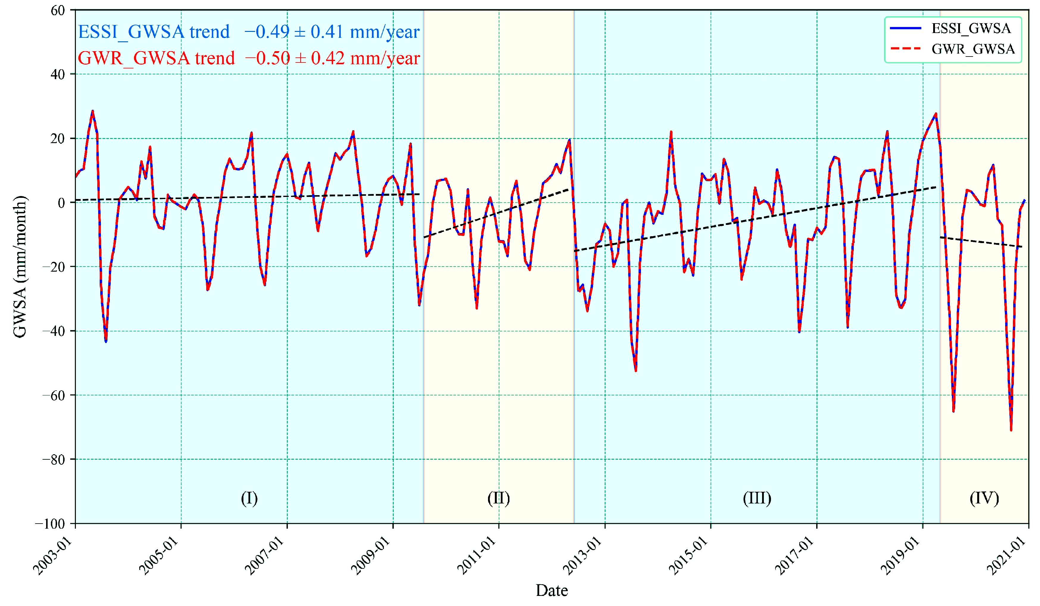
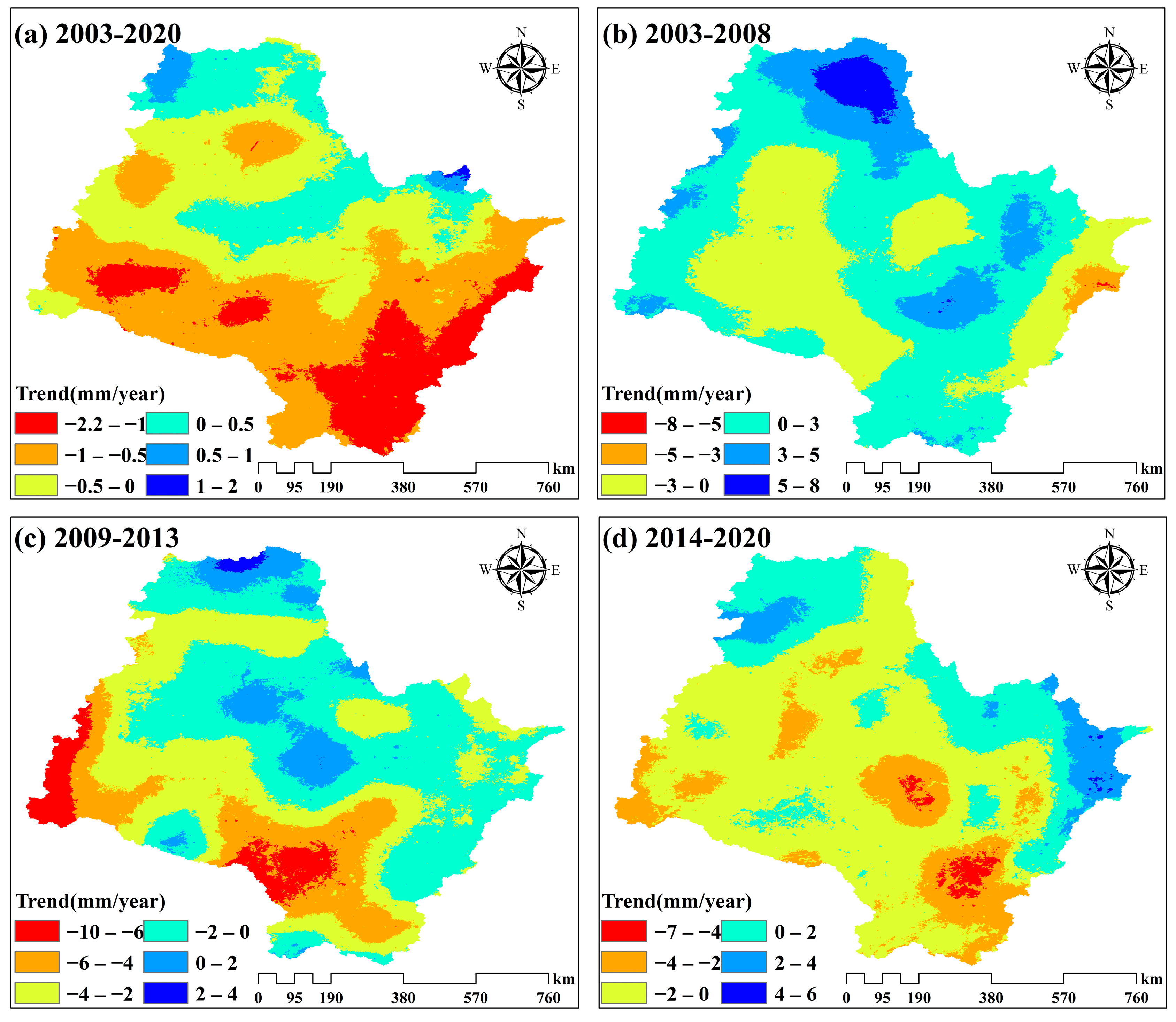
5.2. Analysis of GWSA Change Trend in the Songhua River Basin
5.3. Analysis of LULC and GWSA Changes
5.4. Limitations and Research Prospects
6. Conclusions
Author Contributions
Funding
Data Availability Statement
Acknowledgments
Conflicts of Interest
References
- Arshad, A.; Zhang, Z.; Zhang, W.; Dilawar, A. Mapping Favorable Groundwater Potential Recharge Zones Using a GIS-Based Analytical Hierarchical Process and Probability Frequency Ratio Model: A Case Study from an Agro-Urban Region of Pakistan. Geosci. Front. 2020, 11, 1805–1819. [Google Scholar] [CrossRef]
- Chen, H.; Zhang, W.; Nie, N.; Guo, Y. Long-Term Groundwater Storage Variations Estimated in the Songhua River Basin by Using GRACE Products, Land Surface Models, and in-Situ Observations. Sci. Total Environ. 2019, 649, 372–387. [Google Scholar] [CrossRef] [PubMed]
- Famiglietti, J.S. The Global Groundwater Crisis. Nat. Clim. Chang. 2014, 4, 945–948. [Google Scholar] [CrossRef]
- Yari, A.; Ardalan, A.; Ostadtaghizadeh, A.; Zarezadeh, Y.; Boubakran, M.S.; Bidarpoor, F.; Rahimiforoushani, A. Underlying Factors Affecting Death Due to Flood in Iran: A Qualitative Content Analysis. Int. J. Disaster Risk Reduct. 2019, 40, 101258. [Google Scholar] [CrossRef]
- Cuthbert, M.O.; Gleeson, T.; Moosdorf, N.; Befus, K.M.; Schneider, A.; Hartmann, J.; Lehner, B. Global Patterns and Dynamics of Climate–Groundwater Interactions. Nat. Clim. Chang. 2019, 9, 137–141. [Google Scholar] [CrossRef]
- Zhao, Q.; Zhang, B.; Yao, Y.; Wu, W.; Meng, G.; Chen, Q. Geodetic and Hydrological Measurements Reveal the Recent Acceleration of Groundwater Depletion in North China Plain. J. Hydrol. 2019, 575, 1065–1072. [Google Scholar] [CrossRef]
- Ostad-Ali-Askari, K.; Shayannejad, M. Quantity and Quality Modelling of Groundwater to Manage Water Resources in Isfahan-Borkhar Aquifer. Environ. Dev. Sustain. 2021, 23, 15943–15959. [Google Scholar] [CrossRef]
- Rodell, M.; Famiglietti, J.S.; Wiese, D.N.; Reager, J.T.; Beaudoing, H.K.; Landerer, F.W.; Lo, M.-H. Emerging Trends in Global Freshwater Availability. Nature 2018, 557, 651–659. [Google Scholar] [CrossRef]
- Khan, A.A.; Zhao, Y.; Khan, J.; Rahman, G.; Rafiq, M.; Moazzam, M.F.U. Spatial and Temporal Analysis of Rainfall and Drought Condition in Southwest Xinjiang in Northwest China, Using Various Climate Indices. Earth Syst. Environ. 2021, 5, 201–216. [Google Scholar] [CrossRef]
- Valipour, M.; Bateni, S.M.; Jun, C. Global Surface Temperature: A New Insight. Climate 2021, 9, 81. [Google Scholar] [CrossRef]
- Rodell, M.; Chen, J.; Kato, H.; Famiglietti, J.S.; Nigro, J.; Wilson, C.R. Estimating Groundwater Storage Changes in the Mississippi River Basin (USA) Using GRACE. Hydrogeol. J. 2007, 15, 159–166. [Google Scholar] [CrossRef]
- Tapley, B.D.; Watkins, M.M.; Flechtner, F.; Reigber, C.; Bettadpur, S.; Rodell, M.; Sasgen, I.; Famiglietti, J.S.; Landerer, F.W.; Chambers, D.P.; et al. Contributions of GRACE to Understanding Climate Change. Nat. Clim. Chang. 2019, 9, 358–369. [Google Scholar] [CrossRef] [PubMed]
- Famiglietti, J.S.; Lo, M.; Ho, S.L.; Bethune, J.; Anderson, K.J.; Syed, T.H.; Swenson, S.C.; de Linage, C.R.; Rodell, M. Satellites Measure Recent Rates of Groundwater Depletion in California’s Central Valley. Geophys. Res. Lett. 2011, 38. [Google Scholar] [CrossRef]
- Yin, W.; Zhang, G.; Han, S.-C.; Yeo, I.-Y.; Zhang, M. Improving the Resolution of GRACE-Based Water Storage Estimates Based on Machine Learning Downscaling Schemes. J. Hydrol. 2022, 613, 128447. [Google Scholar] [CrossRef]
- Bierkens, M.F.P.; Wada, Y. Non-Renewable Groundwater Use and Groundwater Depletion: A Review. Environ. Res. Lett. 2019, 14, 063002. [Google Scholar] [CrossRef]
- Chen, J.; Famigliett, J.S.; Scanlon, B.R.; Rodell, M. Groundwater Storage Changes: Present Status from GRACE Observations. Surv. Geophys. 2016, 37, 397–417. [Google Scholar] [CrossRef]
- Ali, S.; Ran, J.; Luan, Y.; Khorrami, B.; Xiao, Y.; Tangdamrongsub, N. The GWR Model-Based Regional Downscaling of GRACE/GRACE-FO Derived Groundwater Storage to Investigate Local-Scale Variations in the North China Plain. Sci. Total Environ. 2024, 908, 168239. [Google Scholar] [CrossRef] [PubMed]
- Yang, X.; Tian, S.; Feng, W.; Ran, J.; You, W.; Jiang, Z.; Gong, X. Spatio-Temporal Evaluation of Water Storage Trends from Hydrological Models over Australia Using GRACE Mascon Solutions. Remote Sens. 2020, 12, 3578. [Google Scholar] [CrossRef]
- Ali, S.; Liu, D.; Fu, Q.; Cheema, M.J.M.; Pal, S.C.; Arshad, A.; Pham, Q.B.; Zhang, L. Constructing High-Resolution Groundwater Drought at Spatio-Temporal Scale Using GRACE Satellite Data Based on Machine Learning in the Indus Basin. J. Hydrol. 2022, 612, 128295. [Google Scholar] [CrossRef]
- Khorrami, B.; Ali, S.; Gündüz, O. Investigating the Local-Scale Fluctuations of Groundwater Storage by Using Downscaled GRACE/GRACE-FO JPL Mascon Product Based on Machine Learning (ML) Algorithm. Water Resour. Manag. 2023, 37, 3439–3456. [Google Scholar] [CrossRef]
- Ran, J.; Ditmar, P.; Liu, L.; Xiao, Y.; Klees, R.; Tang, X. Analysis and Mitigation of Biases in Greenland Ice Sheet Mass Balance Trend Estimates From GRACE Mascon Products. J. Geophys. Res. Solid Earth 2021, 126, e2020JB020880. [Google Scholar] [CrossRef]
- Rodell, M.; Velicogna, I.; Famiglietti, J.S. Satellite-Based Estimates of Groundwater Depletion in India. Nature 2009, 460, 999–1002. [Google Scholar] [CrossRef] [PubMed]
- Long, D.; Yang, Y.; Wada, Y.; Hong, Y.; Liang, W.; Chen, Y.; Yong, B.; Hou, A.; Wei, J.; Chen, L. Deriving Scaling Factors Using a Global Hydrological Model to Restore GRACE Total Water Storage Changes for China’s Yangtze River Basin. Remote Sens. Environ. 2015, 168, 177–193. [Google Scholar] [CrossRef]
- Huang, Z.; Pan, Y.; Gong, H.; Yeh, P.J.-F.; Li, X.; Zhou, D.; Zhao, W. Subregional-Scale Groundwater Depletion Detected by GRACE for Both Shallow and Deep Aquifers in North China Plain. Geophys. Res. Lett. 2015, 42, 1791–1799. [Google Scholar] [CrossRef]
- Tangdamrongsub, N.; Han, S.-C.; Tian, S.; Müller Schmied, H.; Sutanudjaja, E.H.; Ran, J.; Feng, W. Evaluation of Groundwater Storage Variations Estimated from GRACE Data Assimilation and State-of-the-Art Land Surface Models in Australia and the North China Plain. Remote Sens. 2018, 10, 483. [Google Scholar] [CrossRef]
- Nourani, V.; Jabbarian Paknezhad, N.; Ng, A.; Wen, Z.; Dabrowska, D.; Üzelaltınbulat, S. Application of the Machine Learning Methods for GRACE Data Based Groundwater Modeling, a Systematic Review. Groundw. Sustain. Dev. 2024, 25, 101113. [Google Scholar] [CrossRef]
- Liu, D.; Mishra, A.K.; Yu, Z.; Lü, H.; Li, Y. Support Vector Machine and Data Assimilation Framework for Groundwater Level Forecasting Using GRACE Satellite Data. J. Hydrol. 2021, 603, 126929. [Google Scholar] [CrossRef]
- Lopez, T.; Al Bitar, A.; Biancamaria, S.; Güntner, A.; Jäggi, A. On the Use of Satellite Remote Sensing to Detect Floods and Droughts at Large Scales. Surv. Geophys. 2020, 41, 1461–1487. [Google Scholar] [CrossRef]
- Yin, J.; Gentine, P.; Slater, L.; Gu, L.; Pokhrel, Y.; Hanasaki, N.; Guo, S.; Xiong, L.; Schlenker, W. Future Socio-Ecosystem Productivity Threatened by Compound Drought–Heatwave Events. Nat. Sustain. 2023, 6, 259–272. [Google Scholar] [CrossRef]
- Frappart, F.; Papa, F.; Famiglietti, J.S.; Prigent, C.; Rossow, W.B.; Seyler, F. Interannual Variations of River Water Storage from a Multiple Satellite Approach: A Case Study for the Rio Negro River Basin. J. Geophys. Res. Atmos. 2008, 113. [Google Scholar] [CrossRef]
- Hasan, E.; Tarhule, A.; Kirstetter, P.-E. Twentieth and Twenty-First Century Water Storage Changes in the Nile River Basin from GRACE/GRACE-FO and Modeling. Remote Sens. 2021, 13, 953. [Google Scholar] [CrossRef]
- Bolaños, S.; Salazar, J.F.; Betancur, T.; Werner, M. GRACE Reveals Depletion of Water Storage in Northwestern South America between ENSO Extremes. J. Hydrol. 2021, 596, 125687. [Google Scholar] [CrossRef]
- Cazenave, A.; Chen, J. Time-Variable Gravity from Space and Present-Day Mass Redistribution in theEarth System. Earth Planet. Sci. Lett. 2010, 298, 263–274. [Google Scholar] [CrossRef]
- Chen, J.L.; Wilson, C.R.; Tapley, B.D. Contribution of Ice Sheet and Mountain Glacier Melt to Recent Sea Level Rise. Nat. Geosci. 2013, 6, 549–552. [Google Scholar] [CrossRef]
- Liu, B.; Zou, X.; Yi, S.; Sneeuw, N.; Li, J.; Cai, J. Reconstructing GRACE-like Time Series of High Mountain Glacier Mass Anomalies. Remote Sens. Environ. 2022, 280, 113177. [Google Scholar] [CrossRef]
- Zhang, X.; Ren, L.; Feng, W. Comparison of the Shallow Groundwater Storage Change Estimated by a Distributed Hydrological Model and GRACE Satellite Gravimetry in a Well-Irrigated Plain of the Haihe River Basin, China. J. Hydrol. 2022, 610, 127799. [Google Scholar] [CrossRef]
- Feng, W.; Zhong, M.; Lemoine, J.-M.; Biancale, R.; Hsu, H.-T.; Xia, J. Evaluation of Groundwater Depletion in North China Using the Gravity Recovery and Climate Experiment (GRACE) Data and Ground-Based Measurements. Water Resour. Res. 2013, 49, 2110–2118. [Google Scholar] [CrossRef]
- Amiri, V.; Ali, S.; Sohrabi, N. Estimating the Spatio-Temporal Assessment of GRACE/GRACE-FO Derived Groundwater Storage Depletion and Validation with in-Situ Water Quality Data (Yazd Province, Central Iran). J. Hydrol. 2023, 620, 129416. [Google Scholar] [CrossRef]
- Khorrami, B.; Gunduz, O. An Enhanced Water Storage Deficit Index (EWSDI) for Drought Detection Using GRACE Gravity Estimates. J. Hydrol. 2021, 603, 126812. [Google Scholar] [CrossRef]
- Li, F.; Kusche, J.; Chao, N.; Wang, Z.; Löcher, A. Long-Term (1979-Present) Total Water Storage Anomalies Over the Global Land Derived by Reconstructing GRACE Data. Geophys. Res. Lett. 2021, 48, e2021GL093492. [Google Scholar] [CrossRef]
- Ghobadi-Far, K.; Han, S.-C.; Allgeyer, S.; Tregoning, P.; Sauber, J.; Behzadpour, S.; Mayer-Gürr, T.; Sneeuw, N.; Okal, E. GRACE Gravitational Measurements of Tsunamis after the 2004, 2010, and 2011 Great Earthquakes. J. Geod. 2020, 94, 65. [Google Scholar] [CrossRef]
- Sun, Z.; Long, D.; Yang, W.; Li, X.; Pan, Y. Reconstruction of GRACE Data on Changes in Total Water Storage Over the Global Land Surface and 60 Basins. Water Resour. Res. 2020, 56, e2019WR026250. [Google Scholar] [CrossRef]
- Li, F.; Kusche, J.; Rietbroek, R.; Wang, Z.; Forootan, E.; Schulze, K.; Lück, C. Comparison of Data-Driven Techniques to Reconstruct (1992–2002) and Predict (2017–2018) GRACE-Like Gridded Total Water Storage Changes Using Climate Inputs. Water Resour. Res. 2020, 56, e2019WR026551. [Google Scholar] [CrossRef]
- Mukherjee, A.; Ramachandran, P. Prediction of GWL with the Help of GRACE TWS for Unevenly Spaced Time Series Data in India: Analysis of Comparative Performances of SVR, ANN and LRM. J. Hydrol. 2018, 558, 647–658. [Google Scholar] [CrossRef]
- Sun, A.Y.; Scanlon, B.R.; Zhang, Z.; Walling, D.; Bhanja, S.N.; Mukherjee, A.; Zhong, Z. Combining Physically Based Modeling and Deep Learning for Fusing GRACE Satellite Data: Can We Learn From Mismatch? Water Resour. Res. 2019, 55, 1179–1195. [Google Scholar] [CrossRef]
- Lai, Y.; Zhang, B.; Yao, Y.; Liu, L.; Yan, X.; He, Y.; Ou, S. Reconstructing the Data Gap between GRACE and GRACE Follow-on at the Basin Scale Using Artificial Neural Network. Sci. Total Environ. 2022, 823, 153770. [Google Scholar] [CrossRef]
- Wang, F.; Shen, Y.; Chen, Q.; Wang, W. Bridging the Gap between GRACE and GRACE Follow-on Monthly Gravity Field Solutions Using Improved Multichannel Singular Spectrum Analysis. J. Hydrol. 2021, 594, 125972. [Google Scholar] [CrossRef]
- Yi, S.; Sneeuw, N. Filling the Data Gaps Within GRACE Missions Using Singular Spectrum Analysis. J. Geophys. Res. Solid Earth 2021, 126, e2020JB021227. [Google Scholar] [CrossRef]
- Gauer, L.-M.; Chanard, K.; Fleitout, L. Data-Driven Gap Filling and Spatio-Temporal Filtering of the GRACE and GRACE-FO Records. J. Geophys. Res. Solid Earth 2023, 128, e2022JB025561. [Google Scholar] [CrossRef]
- Chen, Z.; Zheng, W.; Yin, W.; Li, X.; Zhang, G.; Zhang, J. Improving the Spatial Resolution of GRACE-Derived Terrestrial Water Storage Changes in Small Areas Using the Machine Learning Spatial Downscaling Method. Remote Sens. 2021, 13, 4760. [Google Scholar] [CrossRef]
- Wang, S.; Cui, G.; Li, X.; Liu, Y.; Li, X.; Tong, S.; Zhang, M. GRACE Satellite-Based Analysis of Spatiotemporal Evolution and Driving Factors of Groundwater Storage in the Black Soil Region of Northeast China. Remote Sens. 2023, 15, 704. [Google Scholar] [CrossRef]
- Watkins, M.M.; Wiese, D.N.; Yuan, D.-N.; Boening, C.; Landerer, F.W. Improved Methods for Observing Earth’s Time Variable Mass Distribution with GRACE Using Spherical Cap Mascons. J. Geophys. Res. Solid Earth 2015, 120, 2648–2671. [Google Scholar] [CrossRef]
- Zheng, L.; Pan, Y.; Gong, H.; Huang, Z.; Zhang, C. Comparing Groundwater Storage Changes in Two Main Grain Producing Areas in China: Implications for Sustainable Agricultural Water Resources Management. Remote Sens. 2020, 12, 2151. [Google Scholar] [CrossRef]
- Akhtar, F.; Nawaz, R.A.; Hafeez, M.; Awan, U.K.; Borgemeister, C.; Tischbein, B. Evaluation of GRACE Derived Groundwater Storage Changes in Different Agro-Ecological Zones of the Indus Basin. J. Hydrol. 2022, 605, 127369. [Google Scholar] [CrossRef]
- Zhang, J.; Liu, K.; Wang, M. Downscaling Groundwater Storage Data in China to a 1-Km Resolution Using Machine Learning Methods. Remote Sens. 2021, 13, 523. [Google Scholar] [CrossRef]
- Atkinson, P.M. Downscaling in Remote Sensing. Int. J. Appl. Earth Obs. Geoinf. 2013, 22, 106–114. [Google Scholar] [CrossRef]
- Yazdian, H.; Salmani-Dehaghi, N.; Alijanian, M. A Spatially Promoted SVM Model for GRACE Downscaling: Using Ground and Satellite-Based Datasets. J. Hydrol. 2023, 626, 130214. [Google Scholar] [CrossRef]
- Fowler, H.J.; Blenkinsop, S.; Tebaldi, C. Linking Climate c Hange Modelling t o Impacts Studies: Recent advances in downscaling t echniques f or hydrological modelling. Int. J. Clim. 2007, 27, 1547–1578. [Google Scholar] [CrossRef]
- Tangdamrongsub, N.; Steele-Dunne, S.C.; Gunter, B.C.; Ditmar, P.G.; Weerts, A.H. Data Assimilation of GRACE Terrestrial Water Storage Estimates into a Regional Hydrological Model of the Rhine River Basin. Hydrol. Earth Syst. Sci. 2015, 19, 2079–2100. [Google Scholar] [CrossRef]
- Tian, S.; Renzullo, L.J.; van Dijk, A.I.J.M.; Tregoning, P.; Walker, J.P. Global Joint Assimilation of GRACE and SMOS for Improved Estimation of Root-Zone Soil Moisture and Vegetation Response. Hydrol. Earth Syst. Sci. 2019, 23, 1067–1081. [Google Scholar] [CrossRef]
- Vishwakarma, B.D.; Zhang, J.; Sneeuw, N. Downscaling GRACE Total Water Storage Change Using Partial Least Squares Regression. Sci. Data 2021, 8, 95. [Google Scholar] [CrossRef] [PubMed]
- Arshad, A.; Mirchi, A.; Vilcaez, J.; Umar Akbar, M.; Madani, K. Reconstructing High-Resolution Groundwater Level Data Using a Hybrid Random Forest Model to Quantify Distributed Groundwater Changes in the Indus Basin. J. Hydrol. 2024, 628, 130535. [Google Scholar] [CrossRef]
- Chen, L.; He, Q.; Liu, K.; Li, J.; Jing, C. Downscaling of GRACE-Derived Groundwater Storage Based on the Random Forest Model. Remote Sens. 2019, 11, 2979. [Google Scholar] [CrossRef]
- Zuo, J.; Xu, J.; Chen, Y.; Li, W. Downscaling Simulation of Groundwater Storage in the Tarim River Basin in Northwest China Based on GRACE Data. Phys. Chem. Earth Parts ABC 2021, 123, 103042. [Google Scholar] [CrossRef]
- Yin, W.; Hu, L.; Zhang, M.; Wang, J.; Han, S.-C. Statistical Downscaling of GRACE-Derived Groundwater Storage Using ET Data in the North China Plain. J. Geophys. Res. Atmos. 2018, 123, 5973–5987. [Google Scholar] [CrossRef]
- Sahour, H.; Sultan, M.; Vazifedan, M.; Abdelmohsen, K.; Karki, S.; Yellich, J.A.; Gebremichael, E.; Alshehri, F.; Elbayoumi, T.M. Statistical Applications to Downscale GRACE-Derived Terrestrial Water Storage Data and to Fill Temporal Gaps. Remote Sens. 2020, 12, 533. [Google Scholar] [CrossRef]
- Yin, W.; Zhang, G.; Liu, F.; Zhang, D.; Zhang, X.; Chen, S. Improving the Spatial Resolution of GRACE-Based Groundwater Storage Estimates Using a Machine Learning Algorithm and Hydrological Model. Hydrogeol. J. 2022, 30, 947–963. [Google Scholar] [CrossRef]
- Li, F.; Zhang, G.; Xu, Y.J. Assessing Climate Change Impacts on Water Resources in the Songhua River Basin. Water 2016, 8, 420. [Google Scholar] [CrossRef]
- Song, X.; Song, S.; Sun, W.; Mu, X.; Wang, S.; Li, J.; Li, Y. Recent Changes in Extreme Precipitation and Drought over the Songhua River Basin, China, during 1960–2013. Atmos. Res. 2015, 157, 137–152. [Google Scholar] [CrossRef]
- Zhang, B.; Liu, C.; Zhang, Z.; Xiong, S.; Zhang, W.; Li, Z.; An, B.; Wang, S. Downscaling and Calibration Analysis of Precipitation Data in the Songhua River Basin Using the GWRK Model and Rain Gauges. IEEE J. Sel. Top. Appl. Earth Obs. Remote Sens. 2024, 17, 12842–12853. [Google Scholar] [CrossRef]
- Li, F.; Zhang, G.; Xu, Y.J. Spatiotemporal Variability of Climate and Streamflow in the Songhua River Basin, Northeast China. J. Hydrol. 2014, 514, 53–64. [Google Scholar] [CrossRef]
- Khorrami, B.; Ali, S.; Abadi, L.H.; Jehanzaib, M. Spatio-Temporal Variations in Characteristics of Terrestrial Water Storage and Associated Drought over Different Geographic Regions of Türkiye. Earth Sci. Inform. 2023, 16, 717–731. [Google Scholar] [CrossRef]
- Khorrami, B.; Gunduz, O. Evaluation of the Temporal Variations of Groundwater Storage and Its Interactions with Climatic Variables Using GRACE Data and Hydrological Models: A Study from Turkey. Hydrol. Process. 2021, 35, e14076. [Google Scholar] [CrossRef]
- Khorrami, B.; Ali, S.; Sahin, O.G.; Gunduz, O. MODEL-COUPLED GRACE-BASED Analysis of Hydrological Dynamics of Drying Lake Urmia and Its Basin. Hydrol. Process. 2023, 37, e14893. [Google Scholar] [CrossRef]
- Rodell, M.; Houser, P.R.; Jambor, U.; Gottschalck, J.; Mitchell, K.; Meng, C.-J.; Arsenault, K.; Cosgrove, B.; Radakovich, J.; Bosilovich, M.; et al. The Global Land Data Assimilation System. Bull. Am. Meteorol. Soc. 2004, 85, 381–394. [Google Scholar] [CrossRef]
- Pekel, J.-F.; Cottam, A.; Gorelick, N.; Belward, A.S. High-Resolution Mapping of Global Surface Water and Its Long-Term Changes. Nature 2016, 540, 418–422. [Google Scholar] [CrossRef]
- Chen, H. Hydrological Processes and Wetlands Distribution under Climate Change in the Amur River Basin: Impacts and Predictions. Ph.D. Thesis, Aerospace Information Research Institute, Chinese Academy of Sciences, Beijing, China, 2020. [Google Scholar]
- Zhang, D.; Zhang, W. Study of Distributed Hydrological Model with the Dynamic Integration of Infiltration Excess and Saturated Excess Water Yielding Mechanism. Dr. Nanjing Nanjing Univ. 2006, 529, 190. [Google Scholar]
- Liu, C.; Xu, C.; Zhang, Z.; Xiong, S.; Zhang, W.; Zhang, B.; Chen, H.; Xu, Y.; Wang, S. Modeling Hydrological Consequences of 21st-Century Climate and Land Use/Land Cover Changes in a Mid-High Latitude Watershed. Geosci. Front. 2024, 15, 101819. [Google Scholar] [CrossRef]
- Liu, Y.; Zhang, W.; Zhang, Z. A Conceptual Data Model Coupling with Physically-Based Distributed Hydrological Models Based on Catchment Discretization Schemas. J. Hydrol. 2015, 530, 206–215. [Google Scholar] [CrossRef]
- Wang, S.; Xu, C.; Zhang, W.; Chen, H.; Zhang, B. Human-Induced Water Loss from Closed Inland Lakes: Hydrological Simulations in China’s Daihai Lake. J. Hydrol. 2022, 607, 127552. [Google Scholar] [CrossRef]
- Xu, C.; Zhang, W.; Wang, S.; Chen, H.; Azzam, A.; Zhang, B.; Xu, Y.; Nie, N. Spatiotemporal Green Water Dynamics and Their Responses to Variations of Climatic and Underlying Surface Factors: A Case Study in the Sanjiang Plain, China. J. Hydrol. Reg. Stud. 2023, 45, 101303. [Google Scholar] [CrossRef]
- Zhang, D.; Zhang, W. Distributed Hydrological Modeling Study with the Dynamic Water Yielding Mechanism and RS/GIS Techniques. In Remote Sensing for Agriculture, Ecosystems, and Hydrology VIII; SPIE: Stockholm, Sweden, 2006; Volume 6359, pp. 340–351. [Google Scholar]
- Khorrami, B.; Pirasteh, S.; Ali, S.; Sahin, O.G.; Vaheddoost, B. Statistical Downscaling of GRACE TWSA Estimates to a 1-Km Spatial Resolution for a Local-Scale Surveillance of Flooding Potential. J. Hydrol. 2023, 624, 129929. [Google Scholar] [CrossRef]
- Senay, G.B.; Budde, M.; Verdin, J.P.; Melesse, A.M. A Coupled Remote Sensing and Simplified Surface Energy Balance Approach to Estimate Actual Evapotranspiration from Irrigated Fields. Sensors 2007, 7, 979–1000. [Google Scholar] [CrossRef]
- Li, Q.; Shi, G.; Shangguan, W.; Nourani, V.; Li, J.; Li, L.; Huang, F.; Zhang, Y.; Wang, C.; Wang, D.; et al. A 1 Km Daily Soil Moisture Dataset over China Using in Situ Measurement and Machine Learning. Earth Syst. Sci. Data 2022, 14, 5267–5286. [Google Scholar] [CrossRef]
- Shangguan, W.; Li, Q.; Shi, G. A 1-Km Daily Soil Moisture Dataset over China Based on in-Situ Measurement (2000–2020); National Tibetan Plateau Data Center [Data Set]: Guangzhoug, China, 2022. [Google Scholar]
- Ding, Y.; Peng, S. Spatiotemporal Trends and Attribution of Drought across China from 1901–2100. Sustainability 2020, 12, 477. [Google Scholar] [CrossRef]
- Peng, S. Spatiotemporal Change and Trend Analysis of Potential Evapotranspiration over the Loess Plateau of China during 2011–2100. Agric. For. Meteorol. 2017, 233, 183–194. [Google Scholar] [CrossRef]
- Peng, S.; Ding, Y.; Liu, W.; Li, Z. 1 Km Monthly Temperature and Precipitation Dataset for China from 1901 to 2017. Earth Syst. Sci. Data 2019, 11, 1931–1946. [Google Scholar] [CrossRef]
- Peng, S. 1-Km Monthly Mean Temperature Dataset for China (1901–2021); A Big Earth Data Platform for Three Poles: Lanzhou, China, 2019. [Google Scholar] [CrossRef]
- Arshad, A.; Mirchi, A.; Taghvaeian, S.; AghaKouchak, A. Downscaled-GRACE Data Reveal Anthropogenic and Climate-Induced Water Storage Decline Across the Indus Basin. Water Resour. Res. 2024, 60, e2023WR035882. [Google Scholar] [CrossRef]
- Abdi, H. Partial Least Squares Regression and Projection on Latent Structure Regression (PLS Regression). WIREs Comput. Stat. 2010, 2, 97–106. [Google Scholar] [CrossRef]
- Vinzi, V.E. Handbook of Partial Least Squares; Springer: Berlin/Heidelberg, Germany, 2010. [Google Scholar]
- Woldesenbet, T.A.; Elagib, N.A.; Ribbe, L.; Heinrich, J. Hydrological Responses to Land Use/Cover Changes in the Source Region of the Upper Blue Nile Basin, Ethiopia. Sci. Total Environ. 2017, 575, 724–741. [Google Scholar] [CrossRef]
- Wang, F.; Shen, Y.; Chen, T.; Chen, Q.; Li, W. Improved Multichannel Singular Spectrum Analysis for Post-Processing GRACE Monthly Gravity Field Models. Geophys. J. Int. 2020, 223, 825–839. [Google Scholar] [CrossRef]
- Ghil, M.; Allen, M.R.; Dettinger, M.D.; Ide, K.; Kondrashov, D.; Mann, M.E.; Robertson, A.W.; Saunders, A.; Tian, Y.; Varadi, F.; et al. ADVANCED SPECTRAL METHODS FOR CLIMATIC TIME SERIES. Rev. Geophys. 2002, 40. [Google Scholar] [CrossRef]
- Walwer, D.; Calais, E.; Ghil, M. Data-adaptive Detection of Transient Deformation in Geodetic Networks. J. Geophys. Res. Solid Earth 2016, 121, 2129–2152. [Google Scholar] [CrossRef]
- Ali, S.; Liu, D.; Fu, Q.; Cheema, M.J.M.; Pham, Q.B.; Rahaman, M.M.; Dang, T.D.; Anh, D.T. Improving the Resolution of GRACE Data for Spatio-Temporal Groundwater Storage Assessment. Remote Sens. 2021, 13, 3513. [Google Scholar] [CrossRef]
- Breiman, L. Random Forests. Mach. Learn. 2001, 45, 5–32. [Google Scholar] [CrossRef]
- Rahaman, M.M.; Thakur, B.; Kalra, A.; Li, R.; Maheshwari, P. Estimating High-Resolution Groundwater Storage from GRACE: A Random Forest Approach. Environments 2019, 6, 63. [Google Scholar] [CrossRef]
- Brunsdon, C.; Fotheringham, A.S.; Charlton, M.E. Geographically Weighted Regression: A Method for Exploring Spatial Nonstationarity. Geogr. Anal. 1996, 28, 281–298. [Google Scholar] [CrossRef]
- Foody, G.M. Geographical Weighting as a Further Refinement to Regression Modelling: An Example Focused on the NDVI–Rainfall Relationship. Remote Sens. Environ. 2003, 88, 283–293. [Google Scholar] [CrossRef]
- Arshad, A.; Mirchi, A.; Samimi, M.; Ahmad, B. Combining Downscaled-GRACE Data with SWAT to Improve the Estimation of Groundwater Storage and Depletion Variations in the Irrigated Indus Basin (IIB). Sci. Total Environ. 2022, 838, 156044. [Google Scholar] [CrossRef]
- Chen, L.; Zhang, Z.; Liu, C.; Xiong, S.; Zhang, W.; Gao, H.; Yi, Y. Incorporating Glacier Processes into Hydrological Simulations in the Headwaters of the Yangtze and Yellow Rivers. Sci. Total Environ. 2024, 951, 175474. [Google Scholar] [CrossRef]
- Xu, C.; Zhang, Z.; Fu, Z.; Xiong, S.; Chen, H.; Zhang, W.; Wang, S.; Zhang, D.; Lu, H.; Jiang, X. Impacts of Climatic Fluctuations and Vegetation Greening on Regional Hydrological Processes: A Case Study in the Xiaoxinganling Mountains–Sanjiang Plain Region, Northeastern China. Remote Sens. 2024, 16, 2709. [Google Scholar] [CrossRef]
- Chen, H.; Zhang, W.; Gao, H.; Nie, N. Climate Change and Anthropogenic Impacts on Wetland and Agriculture in the Songnen and Sanjiang Plain, Northeast China. Remote Sens. 2018, 10, 356. [Google Scholar] [CrossRef]
- Yan, X.; Zhang, B.; Yao, Y.; Yang, Y.; Li, J.; Ran, Q. GRACE and Land Surface Models Reveal Severe Drought in Eastern China in 2019. J. Hydrol. 2021, 601, 126640. [Google Scholar] [CrossRef]
- Satish Kumar, K.; AnandRaj, P.; Sreelatha, K.; Bisht, D.S.; Sridhar, V. Monthly and Seasonal Drought Characterization Using GRACE-Based Groundwater Drought Index and Its Link to Teleconnections across South Indian River Basins. Climate 2021, 9, 56. [Google Scholar] [CrossRef]
- Hong, Z.; Han, Z.; Li, X.; Long, D.; Tang, G.; Wang, J. Generation of an Improved Precipitation Data Set from Multisource Information over the Tibetan Plateau. J. Hydrometeorol. 2021, 22, 1275–1295. [Google Scholar] [CrossRef]
- Long, D.; Pan, Y.; Zhou, J.; Chen, Y.; Hou, X.; Hong, Y.; Scanlon, B.R.; Longuevergne, L. Global Analysis of Spatiotemporal Variability in Merged Total Water Storage Changes Using Multiple GRACE Products and Global Hydrological Models. Remote Sens. Environ. 2017, 192, 198–216. [Google Scholar] [CrossRef]
- Cao, Y.; Nan, Z.; Cheng, G. GRACE Gravity Satellite Observations of Terrestrial Water Storage Changes for Drought Characterization in the Arid Land of Northwestern China. Remote Sens. 2015, 7, 1021–1047. [Google Scholar] [CrossRef]


| Type | Variable | Data Source | Resolution and Time |
|---|---|---|---|
| Meteorology | Precipitation | ERA5_land (https://www.ecmwf.int/en/forecasts/datasets) (accessed on 15 August 2024) | 0.1°, 1 h, 2000–2020 |
| temperature | |||
| Wind speed | |||
| Surface air pressure | |||
| Surface net solar radiation | |||
| Surface solar radiation | |||
| Relative humidity | |||
| Soil property | Bulk density | SoilGrids (https://www.soilgrids.org) (accessed on 15 August 2024) | 1 km, fixed |
| Clay content mass fraction | |||
| Silt content mass fraction | |||
| Sand content mass fraction | |||
| Vegetation parameter | Leaf area index (LAI) | GLOBMAP LAI (https://zenodo.org/) (accessed on 15 August 2024) | 8 km, 8-day, 2000–2020 |
| Land use/cover (LULC) | Resources and Environment Data Cloud Platform (http://www.resdc.cn) (accessed on 15 August 2024) | 1 km, yearly, 2001–2020 | |
| Tree cover fraction | MODIS (https://lpdaac.usgs.gov) (accessed on 15 August 2024) | 500 m, fixed, 2010 | |
| Others | DEM | SRTMDEM (https://www.gscloud.cn) (accessed on 15 August 2024) Water Yearbook | 90 m, fixed monthly, 2010–2020 |
| Streamflow at Jiamusi and Xiaoergou Stations |
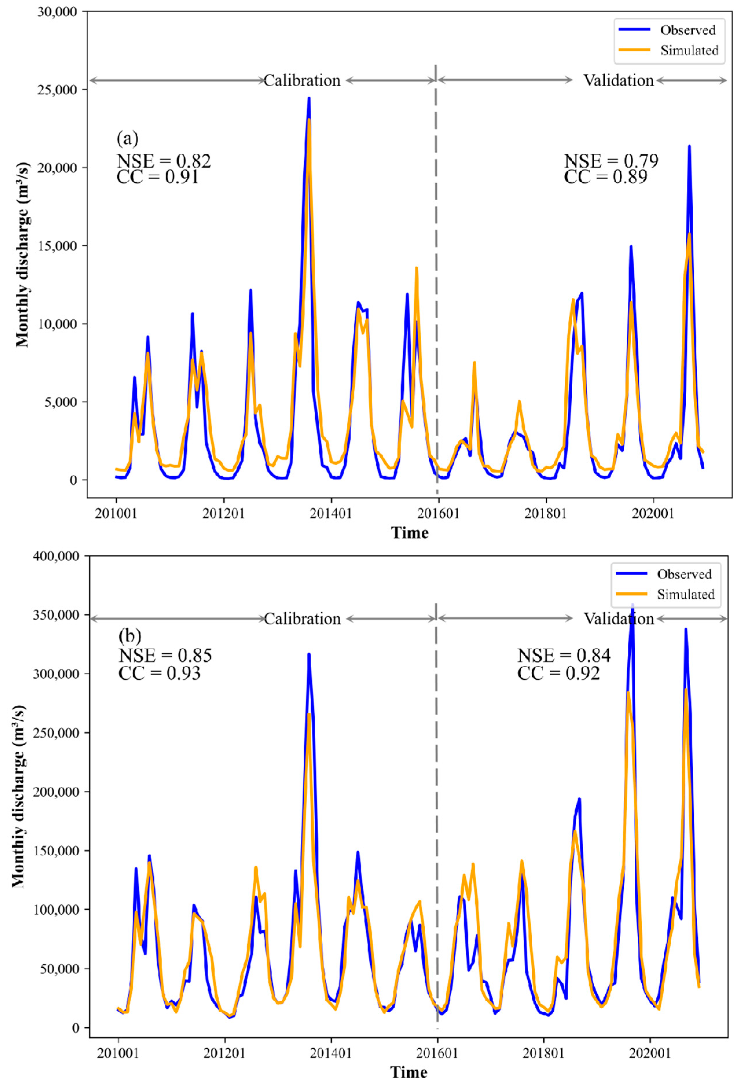
| Hydrological Stations | Calibration (2010–2015) | Validation (2016–2020) | Entire Period (2010–2020) | |||
|---|---|---|---|---|---|---|
| NSE | CC | NSE | CC | NSE | CC | |
| Xiaoergou | 0.82 | 0.91 | 0.79 | 0.89 | 0.81 | 0.90 |
| Jiamusi | 0.85 | 0.93 | 0.84 | 0.92 | 0.84 | 0.93 |
| Grids | GLDAS GWSA | ESSI GWSA | ||
|---|---|---|---|---|
| CC | RMSE | CC | RMSE | |
| A1 | 0.106 | 44.811 | 0.509 | 25.561 |
| A2 | 0.420 | 62.641 | 0.427 | 57.469 |
| A3 | 0.414 | 85.754 | 0.464 | 67.216 |
| A4 | 0.502 | 81.472 | 0.590 | 41.714 |
| A5 | −0.112 | 153.509 | 0.467 | 134.324 |
| A6 | −0.191 | 49.167 | 0.664 | 23.417 |
| A7 | 0.332 | 73.991 | 0.218 | 53.525 |
| A8 | −0.313 | 73.664 | 0.484 | 35.731 |
| A9 | 0.248 | 66.622 | −0.315 | 59.016 |
| CC | NSE | RMSE | |
|---|---|---|---|
| GWR_GWSA | 0.995 | 0.989 | 2.505 |
| RF_GWSA | 0.950 | 0.893 | 7.668 |
| 2003 (km2) | 2020 (km2) | Change Rate (%) | |
|---|---|---|---|
| Crop | 201,245 | 209,316 | 4 |
| Forest | 218,133 | 214,339 | −2 |
| Grassland | 66,556 | 59,437 | −11 |
| Water | 14,341 | 10,545 | −26 |
| Building | 13,644 | 16,462 | 21 |
| Unutilized land | 35,936 | 39,500 | 10 |
Disclaimer/Publisher’s Note: The statements, opinions and data contained in all publications are solely those of the individual author(s) and contributor(s) and not of MDPI and/or the editor(s). MDPI and/or the editor(s) disclaim responsibility for any injury to people or property resulting from any ideas, methods, instructions or products referred to in the content. |
© 2024 by the authors. Licensee MDPI, Basel, Switzerland. This article is an open access article distributed under the terms and conditions of the Creative Commons Attribution (CC BY) license (https://creativecommons.org/licenses/by/4.0/).
Share and Cite
Liu, C.; Zhang, Z.; Xu, C.; Zhang, W. Reconstructing Long-Term, High-Resolution Groundwater Storage Changes in the Songhua River Basin Using Supplemented GRACE and GRACE-FO Data. Remote Sens. 2024, 16, 4566. https://doi.org/10.3390/rs16234566
Liu C, Zhang Z, Xu C, Zhang W. Reconstructing Long-Term, High-Resolution Groundwater Storage Changes in the Songhua River Basin Using Supplemented GRACE and GRACE-FO Data. Remote Sensing. 2024; 16(23):4566. https://doi.org/10.3390/rs16234566
Chicago/Turabian StyleLiu, Chuanqi, Zhijie Zhang, Chi Xu, and Wanchang Zhang. 2024. "Reconstructing Long-Term, High-Resolution Groundwater Storage Changes in the Songhua River Basin Using Supplemented GRACE and GRACE-FO Data" Remote Sensing 16, no. 23: 4566. https://doi.org/10.3390/rs16234566
APA StyleLiu, C., Zhang, Z., Xu, C., & Zhang, W. (2024). Reconstructing Long-Term, High-Resolution Groundwater Storage Changes in the Songhua River Basin Using Supplemented GRACE and GRACE-FO Data. Remote Sensing, 16(23), 4566. https://doi.org/10.3390/rs16234566