Abstract
The radar monopulse angle measurement can obtain a target’s angle information within a single pulse, meaning that factors such as target motion and amplitude fluctuations, which vary over time, do not affect the angle measurement accuracy. However, in practical applications, when a target’s signal-to-noise ratio (SNR) is low, the single pulse signal is severely affected by noise, leading to a significant deterioration in angle measurement accuracy. Therefore, it is usually necessary to coherently integrate multiple pulses before estimating the angle. This paper constructs an angle expansion model for a multi-pulse angle measurement under coherent integration. The analysis reveals that even under noise-free conditions, after coherently integrating multiple pulses, the coupling of target amplitude fluctuations and motion state can still cause significant errors in the angle measurement. Subsequently, this paper conducts a detailed analysis of the impact of the amplitude fluctuations and target maneuvers on the random angle measurement error. It also derives approximate probability density functions of angle measurement errors under various fluctuation and motion scenarios based on the Lindeberg–Feller central limit theorem. In addition, based on the angle expansion model and the random error distribution, this paper proposes an angle correction algorithm based on multi-pulse integration and long-term estimation. Numerical experiments and radar data in the field verify the impact of target characteristics on the angle measurement under multi-pulse integration and the effectiveness of the angle correction algorithm.
1. Introduction
High-precision radar angle measurement is in high demand across various radar detection fields [1], such as low-altitude foreign object warning [2], aircraft navigation management [3], and military target tracking [4]. In recent years, scholars worldwide have made continuous advancements in the development of precise radar angle measurement systems and corresponding algorithms. Early radar systems primarily monitored aircraft in the air, providing directional information through antenna pointing with relatively coarse angle measurements. Subsequently, the emergence of the sequential lobing technique further improved the angle measurement accuracy [5,6]. However, this method requires multiple scans of the target to estimate the angle offset from the scanning normal, and fluctuations in the target echo and movement during the scan can severely affect the angle measurement performance. To address this, researchers proposed the monopulse radar system [7,8]. In this system, the radar antenna can simultaneously form multiple sum and difference beams with different directional patterns, and by comparing the signals from the sum and difference beams, the target’s angular position information can be obtained. Since angle measurements can be performed based on a single pulse, this system is referred to as the monopulse radar system.
Due to the advantages of the monopulse radar, such as the short time required to obtain angle information, high angle measurement accuracy, and strong anti-interference capability, it has been widely used in both military and civilian radar fields. Among the various implementations of the monopulse radar, amplitude comparison monopulse is one of the most common, offering a higher signal-to-noise ratio (SNR), simple structure, and ease of implementation [9]. Consequently, it is widely applied in tracking radars or height-finding radars, and the corresponding amplitude comparison monopulse angle measurement algorithms have become a research hotspot. There is a common consensus in the radar industry that the monopulse radar can obtain the target’s angle information within a single pulse, during which the target’s amplitude and position can be considered constant, and factors such as target motion and amplitude fluctuations, which vary over time, do not affect the accuracy of the monopulse angle measurement. Therefore, current research on angle measurement errors caused by target amplitude fluctuations and movement is limited. High-precision angle measurement studies mainly focus on non-ideal conditions such as multipath effects at low elevation angles [10,11,12,13], angle deviation under jamming [14,15,16,17], and angular separation in multi-target scenarios [18,19,20,21].
However, for weak airborne targets, such as small drones [22], birds, or insects [23,24], the radar echo signals are typically weak, resulting in a low signal-to-noise ratio (SNR) within a single pulse. The interference from noise significantly affects the angle measurement accuracy of the monopulse radar. To address this issue, the multi-pulse integration of radar echo signals can be performed to effectively improve the SNR, thereby reducing the errors introduced by noise. However, multi-pulse integration introduces new challenges for angle measurement, in which during the integration process, the target’s displacement and flight attitude may undergo significant changes, leading to considerable fluctuations in its angle and radar cross-section (RCS). These changes differ from the ideal conditions assumed in previous monopulse angle measurement analyses, where the target’s state is presumed to remain constant over a short period. Target motion and amplitude fluctuations will affect the angle estimation after multi-pulse integration [25]. Quantitatively analyzing the angle measurement errors caused by integration and correcting these errors have become new challenges in angle measurement under multi-pulse integration.
Currently, research on the impact of multi-pulse integration on the accuracy of monopulse radar angle measurements remains scarce. To address these challenges, this chapter constructs an angle expansion model for multi-pulse angle measurement under coherent integration. The analysis reveals that even under noise-free conditions, after coherent integration of multiple pulses, the coupling of target amplitude fluctuations and motion state can still cause significant errors in the angle measurement. Subsequently, this paper conducts a detailed analysis of the impact of the amplitude fluctuations and target maneuvers on this random angle measurement error. Based on the Lindeberg–Feller central limit theorem, approximate probability density functions of angle measurement errors under various fluctuation and motion scenarios are derived. In addition, this paper proposes an angle correction algorithm based on multi-pulse integration and long-term estimation utilizing the angle expansion model and random error distribution. Numerical experiments and field radar data validate both the impact of target characteristics on monopulse angle measurement and the effectiveness of the angle correction algorithm.
The structure of the paper is as follows: Section 2 introduces the basic principles of monopulse angle measurement using the amplitude comparison method and constructs a signal model for amplitude comparison angle measurement under multi-pulse integration. Section 3 develops an angle expansion model for two motion scenarios based on the Lindeberg–Feller central limit theorem and the multi-pulse angle measurement signal model, explaining the impact of target motion and amplitude fluctuations on angle measurement after multi-pulse integration. Section 4 proposes an angle correction algorithm based on multi-pulse integration and long-term estimation, using the angle expansion model of moving targets to correct deviations in the angle measurement caused by multi-pulse integration and enhance angle estimation accuracy. Section 5 validates the accuracy of the proposed angle expansion model and the performance of the angle correction algorithm through simulation experiments. Section 6 evaluates the angle measurement performance of the proposed method using real measurement data. Finally, Section 7 summarizes the content of the paper.
2. Amplitude Comparison Angle Measurement Under Multi-Pulse Integration
2.1. Amplitude Comparison Monopulse Angle Measurement Principles
The monopulse automatic angle measurement is a simultaneous beam angle measurement method. In an angular plane, two identical beams partially overlap, with the overlapping direction being the common signal axis. By comparing the echo signals received simultaneously by these two beams, the angular error signal of the target within this directional plane can be obtained. With the common signal axis of the antenna known, angle measurement can be achieved. Since the two beams receive the echo simultaneously, the time required to obtain the target’s angular error information is very short, theoretically allowing angle error determination with just one echo pulse. The amplitude comparison monopulse angle measurement is one of the most common monopulse angle measurement methods. The essence of the amplitude comparison monopulse method is to use the sum and difference beams of two offset antenna patterns. As shown in Figure 1 below, the sum beam is used for transmission, while the sum and difference beams are used for reception.
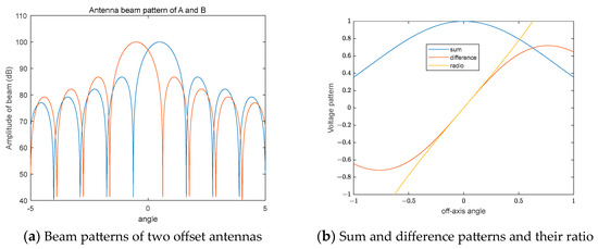
Figure 1.
Beam patterns for the sum and difference beams with two feeds.
Assuming that the antenna’s beam pattern is , and the beam centers of the two feeds are both offset by an angle , from the common signal axis, then the beam patterns of the sum channel and the difference channel can be expressed as follows:
If there is a target with an angle offset from the sum–difference axis of , the received signal in the sum channel is , and the received signal in the difference channel is . When is small, the ratio of the signals in the sum and difference channels is proportional to , as shown in Equation (2):
where represents the slope of the monopulse angle measurement curve.
2.2. Multi-Pulse Integration Angle Measurement Model
In the monopulse amplitude ratio radar system, the central axis of the antenna beam can be set as the axis, and the four horn antennas of A, B, C, and D are placed symmetrically on the plane (as shown in Figure 2a), and the radar antenna coordinate system is established according to Figure 2b.
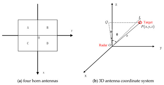
Figure 2.
Radar antenna planar coordinates and 3D antenna coordinate system.
Point is the center of the radar, the offset beams of the four channels are symmetrically aligned with respect to the -axis and -axis, is the center axis of the radar beam, is the target position, and is the radar line of sight to the target. is the projection of point onto the plane, and is the projection of point onto the plane. Thus, and represent the target’s azimuth and elevation angles , respectively, in the radar antenna coordinate system. If the target’s Cartesian coordinates in the antenna coordinate system are , then the relationship between the azimuth error , the elevation error , and the target coordinates is as follows:
Assuming the slopes of the radar azimuth angle error curve and the elevation angle error curve are and , respectively. Within a CPI, there are pulses, and let the sum channel signal of the -th pulse (time) be , with azimuth angle error and elevation angle error . Then, the azimuth difference channel signal and the elevation difference channel signal can be expressed as follows:
For pulses, performing coherent integration on the sum and difference channel signals, respectively, and for simplicity, ignoring noise effects, assuming that after coherent integration, the phase has been optimally compensated. The compensated sum channel signal of the -th pulse becomes , where is a constant. Then, the results of the integrated sum and difference channels are as follows:
Assuming that is a constant and does not change with azimuth angle error or elevation angle error, considering coherent integration, the azimuth angle error is obtained using the amplitude ratio method.
The elevation angle error is similar to the azimuth angle error and can be analyzed in the same way. For simplicity, we will subsequently focus only on the properties of the azimuth angle error obtained using the amplitude ratio method after coherent integration in various motion scenarios.
3. Angle Expansion Model Based on the Lindeberg–Feller Central Limit Theorem
This section integrates the monopulse angle measurement model and the multi-pulse coherent integration model to construct angle measurement models for fluctuating targets after multi-pulse integration under uniform linear motion and uniformly accelerated linear motion scenarios in a three-dimensional space, presented in Section 3.2 and Section 3.3. Furthermore, applying the Lindeberg–Feller central limit theorem introduced in Section 3.1, Section 3.2 and Section 3.3 demonstrate a generalized multi-pulse integration angle expansion model for both uniform and accelerated linear motion scenarios, where under the same motion scenario, regardless of the specific amplitude distribution of the fluctuating target, as long as the expectation and variance of the distributions are identical, the angular error distribution of the multi-pulse integration angle measurement will ultimately converge to the same normal distribution. Based on the theoretical properties of asymptotic normality provided by the Lindeberg–Feller central limit theorem, the expectation and variance of the converged normal distribution in the angle expansion model are also precisely derived.
3.1. Lindeberg–Feller Central Limit Theorem
The central limit theorem is an important application theorem in probability theory [26]. It explains that despite many underlying factors in natural and social sciences having non-normal distributions, the aggregation of multiple factors often approaches a normal distribution. The earliest formal statement of the central limit theorem was proposed by the French mathematician Laplace in the 19th century, describing that if a sufficiently large sample is randomly drawn from a population with an arbitrary distribution, the mean (or sum) of these samples will tend to follow a normal distribution.
The central limit theorem can be defined in the following mathematical form [27], where are the sample values randomly drawn from a population with probability distribution . Then, these sample values are one-dimensional random variables with probability distribution and are mutually independent. The average of these samples, , can be expressed as follows:
Assuming the mean and variance of the probability distribution are and , respectively, the standardized form of the sample mean is defined as follows:
As increases, the standardized sample mean will gradually approach a standard normal distribution , i.e.,:
where represents a standard normal distribution random variable.
Therefore, the normal distribution trend of the central limit theorem does not depend on the shape of the original population distribution. Whether the original data are skewed, flat, or multimodal, this conclusion holds when the sample size is sufficiently large. The importance of the central limit theorem lies in its theoretical foundation for using normal distributions in statistical inference, especially when the sample size is large. In practical applications, even if we know almost nothing about the population distribution, the central limit theorem allows us to approximate the distribution of the sample mean using the properties of the normal distribution, thus enabling hypothesis testing and confidence interval calculation.
However, the standard central limit theorem assumes that all random variables are independently and identically distributed with finite variance. In more general cases, when these assumptions are not fully met, the Lindeberg–Feller central limit theorem provides further extensions [28]. The Lindeberg–Feller central limit theorem describes the relationship between the independent random variables and the central limit theorem under more relaxed conditions. This theorem considers independent but not necessarily identically distributed random variables and uses the Lindeberg condition to ensure convergence.
The mathematical statement of the Lindeberg–Feller central limit theorem is as follows [29]: Let there be one-dimensional random variables , each with probability distributions , and they are mutually independent. The expectation and variance of the -th random variable satisfies
And let
if satisfy the Lindeberg condition, that is, for any ,
where is the indicator function, which is expressed as follows:
Then, for the sum of these random variables, , can be represented by Equation (14).
As increases, the probability distribution of the normalized sum of the random variables will approach a normal distribution with mean 0 and variance .
The Lindeberg–Feller central limit theorem is a further generalization of the traditional central limit theorem and does not require the random variables to have the same distribution. Therefore, it has broader applications in practical statistics. In Section 3.2 and Section 3.3, we will use the Lindeberg–Feller central limit theorem to demonstrate that, in three-dimensional uniform linear motion and three-dimensional uniformly accelerated linear motion scenarios, the angle error distribution of multi-pulse integration will gradually approach a normal distribution, and the variance of this normal distribution will be related to the target’s motion parameters and fluctuation parameters.
3.2. Uniform Linear Motion in Three-Dimensional Space
In Section 2.2, we derived the angle error model for the multi-pulse integration angle measurement. This section will use the three-dimensional uniform linear motion model as a basis to analyze the relationship between the angle error of the target and the number of pulses in this scenario. Subsequently, by combining the angle error model under multi-pulse integration with the Lindeberg–Feller central limit theorem, we can perform modeling and analysis of the angle expansion caused by target amplitude fluctuation and multi-pulse integration in three-dimensional uniform linear motion.
3.2.1. Multi-Pulse Angle Error Model for Uniform Linear Motion
As shown in Figure 2, with the radar’s central axis as the -axis and the four horn antennas forming the plane, we can establish the radar antenna Cartesian coordinate system and spherical coordinate system. Assuming that the target is moving with uniform linear motion in a three-dimensional space, the initial coordinates of the target in the antenna coordinate system are , with three-dimensional velocity components . The Cartesian coordinates of the target in the antenna Cartesian coordinate system at time can be expressed as follows:
In Equation (3), we obtain the relationship between the azimuth angle error and the target’s Cartesian coordinates as follows:
Substituting Equation (15) into Equation (16), since in the actual angle measurements, to satisfy the linear range of the angle measurement curve, and are very small, satisfying and , we have the approximate the relationship between the azimuth angle error at different times and the target’s initial coordinates and three-dimensional velocity components:
where is the length of the projection of the initial slant range of the target onto the plane.
Equation (17) shows that the azimuth angle error can be approximated as varying linearly with time during the integration period. To facilitate the analysis of the subsequent angle expansion model, the azimuth angle errors at each pulse time can be expressed in the form of an arithmetic sequence:
where represents the pulse index, denotes the azimuth angle error of the target at the -th pulse, and and represent the linear and constant terms of the time-varying component in Equation (17), respectively, i.e.,:
where represents the radar’s pulse repetition period.
If there is no fluctuation of the target between pulses, then we assume that the target’s amplitude satisfies the following condition:
where is a constant value, and represents the target amplitude of the -th pulse.
Substituting Equation (20) into Equation (6), we obtain:
According to Equation (18), varies linearly with , thus:
This indicates that the angle error obtained after coherent integration equals the angle error at the middle time, .
3.2.2. Angle Expansion Model Under Amplitude Fluctuation for Uniform Linear Motion
If the target amplitude varies between pulses, we assume that the amplitudes of the individual pulses satisfy the condition of being independent and identically distributed, i.e.,:
where represents the target amplitude of the -th pulse, and denotes a random variable with a certain distribution, having a mean of and a standard deviation of .
Based on Equation (6), we can obtain:
Substituting Equation (18) into Equation (24), we obtain:
For convenience in analysis, we performed a linear transformation on , letting . According to Equation (25), we obtained the following:
The numerator and the denominator of can be viewed as two random variables that are correlated and not independent. This correlation decreases as the total number of integrated pulses increases. In probability theory, the probability density function of the ratio of two random variables involves the convolution of their probability density functions, which makes Equation (26) less suitable for analyzing the trend of ’s probability density function as increases. Therefore, is further decomposed into a linear weighted sum of multiple random variables, i.e.,
where
Although the assumption is that and are independent, is part of the sum , so there is some correlation between the numerator and denominator of . As increases, the proportion of in the overall sum becomes smaller, and the correlation between and decreases. When is large, the numerator and denominator can be approximately independent. Additionally, since and are independent, when is large, and can be seen as and divided by the sum , which is unrelated to them. Therefore, and are approximately independent, meaning that as becomes large, tend to be independent.
Thus, when is large, the expectation and variance of are as follows:
Since the expectation of is not zero, to simplify the proof of the Lindeberg condition, we introduces another random variable , which is equal to minus a constant, as shown in Equation (30).
Thus, has an expectation of 0, with variance and higher-order central moments identical to those of , and and are independent. Therefore, can be expressed as shown in Equation (31).
can be viewed as the sum of the random variable and the constant . Therefore, by determining the distribution of , we can obtain the distribution of . Thus, we can prove that when the number of integrated pulses is large, the sum of independent but not identically distributed random variables satisfies the Lindeberg condition and can be approximated by a Gaussian distribution.
Since
it is easy to obtain the following:
Therefore, takes bounded values in the range , and the probability of is 0, i.e.,
According to Equations (29) and (11), the sum of the variances of the random variables in the Lindeberg condition is as follows:
It needs to be proven that for any , there is
According to Equation (34), we know that is bounded and does not exceed . Therefore,
and for any , as tends to infinity with increasing , it is sufficient for to be large enough to satisfy . Thus,
Therefore, the sum of the random variables satisfies the Lindeberg condition, and when is large, approaches a Gaussian distribution with a mean of zero and variance .
Furthermore, according to Equation (31) and the properties of the probability theory, when is large, can also be approximated as a Gaussian distribution, where the expectation of , denoted as , is as follows:
Actually, for any , is always equal to , and this does not require the condition of independence between the numerator and denominator when is large (see Appendix A for a detailed proof).
The variance of , denoted , is consistent with :
Thus, the probability density function of is symmetric about (see Appendix A). When the number of integrated pulses is large, the probability density function can be approximated using the Gaussian distribution, according to the Lindeberg–Feller central limit theorem:
Simplifying the above expression yields:
3.3. Uniformly Accelerated Linear Motion in a Three-Dimensional Space
3.3.1. Multi-Pulse Angle Error Model for Uniformly Accelerated Linear Motion
In Equation (3), we obtain the relationship between the azimuth angle error and the target cartesian coordinates as follows:
Since in the practical angle measurement, in order to satisfy the linear range of the measurement curve, and are both very small, satisfying , and , there is an approximate relationship between the azimuth angle error at different times and the target’s initial coordinates, three-dimensional velocity components, and three-dimensional acceleration components, which is expressed as the following:
where the constant , represents the length of the projection of the initial slant range between the target and the radar onto the plane, is the velocity component of the target along the axis, is the acceleration component of the target along the axis, and is the velocity component of the target along the axis.
From the quadratic term coefficient in the Equation (44), it can be seen that when is large or is small, the influence of the quadratic term is greater. During the integration time, the azimuth error can approximately change parabolically with time. Therefore, the azimuth error at each pulse time can be expressed in the form of a quadratic term.
where represents the pulse sequence number, represents the azimuth error of the target at the -th pulse, and , , and represent the quadratic term, linear term, and constant term that vary with time as given in Equation (44).
where represents the radar’s pulse repetition period.
3.3.2. Angle Expansion Model Under Amplitude Fluctuation in Uniformly Accelerated Linear Motion
If there is no fluctuation in the target amplitude between pulses, it is assumed that the target amplitude satisfies the following conditions:
where represents the target amplitude of the -th pulse.
Substitute Equations (47) and (45) into Equation (6), we obtain the following:
The expression for the angular error at the center moment is as follows:
If the target amplitude varies between pulses, assume that the amplitudes of the individual pulses satisfy the condition of being independent and identically distributed, i.e.,
where represents the target amplitude of the -th pulse, and denotes a random variable with a certain distribution, having a mean of and a standard deviation of .
Substitute Equation (45) into (6) to obtain:
Similarly to the derivation in Section 3.2.2, using the Lindeberg–Feller central limit theorem, when the number of integrated pulses is large, can be approximated by a Gaussian distribution, as follows:
can be decomposed as shown in Equation (52):
where
For , since and are independent, as increases, the correlation between and decreases. When is large, the numerator and denominator of can be approximately independent. Moreover, since and are independent, and are approximately independent, meaning that as becomes large, tend to be independent. Therefore, when is large, the expectation and variance of are as follows:
At the same time, based on the expression of in Equation (53), we can obtain the boundedness of :
As similarly described in Section 3.2.2, we can use the boundedness of to prove that satisfies the Lindeberg condition. Therefore, when is large, can also be approximated by a Gaussian distribution. The expectation and variance of can be determined using the independence conditions and the Lindeberg–Feller theorem, which gives:
where
Thus, when the target undergoes a uniformly accelerated linear motion, the multi-pulse integrated angle measurement error can be approximated as following a Gaussian distribution:
Analyzing the probability model of leads to the following conclusions:
- From the mean component, it can be observed that the angular error after multi-pulse integration is greater than the angular error at the central moment , with the difference being ; as increases, this deviation gradually grows.
- From the variance component, it is evident that the greater the target fluctuation, the greater the impact of integration on angular error measurement; as the number of integrated pulses increases, the impact on angular error measurement also increases.
- Overall, when the quadratic term coefficient of angular error variation in Equation (58), it can be reduced to Equation (42) in Section 3.2 under uniform velocity conditions.
4. Angle Correction Algorithm Based on Multi-Pulse Integration and Long-Term Estimation
In practical radar applications, low signal-to-noise ratio (SNR) targets such as small drones, birds, and insects are highly affected by noise interference. Monopulse radar has difficulty achieving high-precision angle measurements for small targets within a single pulse. To reduce the impact of noise on angle measurement, it is typically necessary to perform multi-pulse coherent integration of the target echoes to ensure the accuracy of the angle measurement. However, as concluded in Section 3, during multi-pulse coherent integration, the target’s intense motion and amplitude variations can introduce non-negligible random fluctuation errors in the angle measurement results. To address this issue, based on the two angular spread models under the Gaussian approximation derived in Section 3, this paper proposes an angle correction algorithm based on multi-pulse integration and long-term estimation under the scenarios of uniform linear motion and uniformly accelerated linear motion in three-dimensional space.
4.1. Uniform Linear Motion in Three-Dimensional Space
Assuming that the change in angle varies linearly with time, i.e., , where the two unknown parameters and need to be estimated. Let the number of integrated pulses within a single CPI be , and the signal contains a total of CPIs. In the -th CPI, the integrated measured angle is . As noted in Section 3.2.2, follows a Gaussian distribution, and its expression is as follows:
can also be expressed as:
where is the Gaussian noise that follows .
Since is a univariate linear model with respect to , the slope and intercept can be estimated using the least squares method. The principle of the least squares method is to determine the position of the line by minimizing the sum of squared residuals.
For ease of expression, as shown in Equation (61), the slope is simply denoted as , and the intercept is simply denoted as .
Then, the cost function can be expressed as follows:
To minimize , according to the principle of least squares, the partial derivatives of the cost function with respect to the slope and the intercept should both be zero, as shown in Equation (63):
Substitute Equation (62) into (63) to solve for:
Based on the relationship between , , , and in Equation (61), we can further obtain the following:
4.2. Uniformly Accelerated Linear Motion in a Three-Dimensional Space
Assuming that the change in the angle follows a parabolic relationship with time, i.e., , we need to estimate the three unknown parameters , , and . Let be the number of pulses integrated within a single CPI, and there are CPIs in total. Suppose that in the -th CPI, the integrated measured angle is . As described in Section 3, follows a Gaussian distribution with variance and expectation as follows:
where the expression for is given in Equation (67).
where is the Gaussian noise following .
Similarly, using the least squares method for quadratic curve fitting with respect to , we obtain the coefficients of the quadratic term , the linear term , and the constant term . Combined with Equation (69), we obtain:
According to Equation (70), the estimates for the three unknown parameters , , and are as follows:
5. Simulation Experiment Verification
5.1. Gaussian Approximation of Angle Expansion Models
To validate the accuracy of the angle expansion models derived in Section 3 for scenarios of uniform linear motion and uniformly accelerated linear motion, as shown in Table 1, this paper uses the system parameters of an existing Ku-band high-resolution phased array radar for the simulation experiments (in this radar system, ten sub-pulses with a bandwidth of 125 MHz are synthesized into a 1 GHz wideband radar one-dimensional range profile). The experiments simulate single-pulse angle measurements with target amplitude following five classic probability distributions under both uniform linear motion and uniformly accelerated linear motion scenarios. The five classic probability distributions include the Gamma distribution [24,30], Rayleigh distribution [31,32], Gaussian distribution [33,34], Weibull distribution [35,36], and a mixed Gaussian distribution [37].

Table 1.
Simulation radar system parameters under monopulse angle measurement.
The Kolmogorov–Smirnov (KS) test [38,39] is used to assess the similarity between the Gaussian distribution of the angle expansion model derived in this paper and the angular error probability distribution obtained from multi-pulse integration in the Monte Carlo simulations. Additionally, random noise can also cause fluctuations in angle measurement errors, hence, we need to exclude noise interference to demonstrate that under target motion and fluctuations, monopulse angle measurement still follows a Gaussian distribution after multi-pulse integration. Therefore, no additional noise is added in the simulation experiments for both scenarios, and the variations in the amplitude and phase of the echo signals solely originate from the target’s fluctuations and motion.
5.1.1. Uniform Linear Motion in a Three-Dimensional Space
To verify the validity of the Gaussian approximation of the angle expansion model under various amplitude fluctuation scenarios, as discussed in Section 3.2, we simulated a uniformly linear moving target with a y-axis velocity of 20 m/s and a z-axis velocity of −10 m/s, as shown in Table 2. By substituting the target’s position and velocity into Equations (17) and (18), we found that the angular error changes linearly with the number of pulses, with a slope and intercept of 0.01. The amplitude followed classical distributions: Gamma, Rayleigh, Gaussian, Weibull, and mixed Gaussian distributions. It is worth noting that the mixed Gaussian distribution is obtained by linearly weighting three Gaussian distributions, and its probability density function has three peak points. The weighted values, means, and variances of the three Gaussian distributions are recorded as the weight matrix, mean matrix, and variance matrix, respectively.
Table 2.
Simulation parameters of uniformly moving linear targets.
In the five amplitude fluctuation scenarios, multiple pulse-echo signals were processed using coherent integration, and the angular errors of the single-pulse amplitude comparison measurements were calculated. The number of integrations was 50, and 1 million Monte Carlo simulations were performed to statistically analyze the probability density curves of the angular errors. Then, the mean and variance of each amplitude fluctuation scenario were substituted into the Gaussian approximation Equation (42) of the angle expansion model discussed in Section 3.2. The differences between the probability densities obtained from the Monte Carlo simulations and those derived from the angle expansion model equation were compared, and the differences between the corresponding cumulative distribution functions (CDFs) of the two distributions were calculated, which is the KS test statistic.
Figure 3 compares the probability density curves of single-pulse amplitude comparison angular errors obtained from the Monte Carlo simulations with those derived from the angle expansion model in five different amplitude distribution scenarios. It can be observed that, despite the different types, means, and variances of the amplitude distributions in the five simulation scenarios, the probability density curves obtained by the two methods align very well.
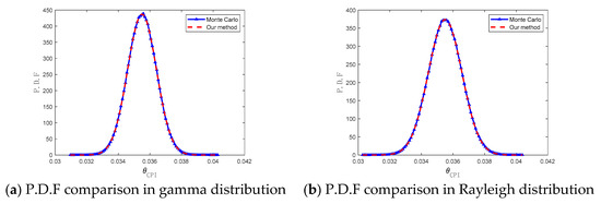
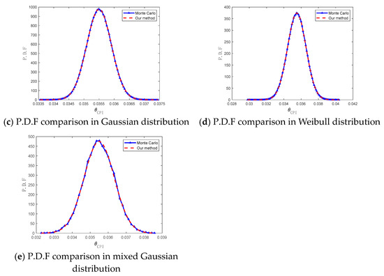
Figure 3.
P.D.F comparison between the Monte Carlo simulation and angle expansion model in uniform linear motion scenario.
To quantitatively assess the differences between the two angular error distributions, we computed the KS distance for the five scenarios, as shown in Table 3. From Table 3, it can be seen that the KS distance is from 1.2 × 10⁻³ to 2.8 × 10⁻³ across the five scenarios, indicating a high degree of similarity between the two distributions. The results of the multiple simulations demonstrate that even without noise interference, amplitude fluctuations and uniform linear motion of the target still cause error fluctuations in the angle measurements obtained through multi-pulse integration. Regardless of the type of amplitude distribution, this error fluctuation tends to approximate the Gaussian distribution when the number of pulses is large.
Table 3.
KS distance of the Monte Carlo simulation statistics and angle expansion model under uniform linear motion scenario.
5.1.2. Uniformly Accelerated Linear Motion in a Three-Dimensional Space
For the three-dimensional uniformly accelerated linear motion scenario, the simulation target parameters are almost identical to those in Section 5.1.1 for the uniform linear motion scenario, except that the acceleration is 20 m/s2. The amplitude still follows the classical distributions listed in Table 2, including the Gamma distribution, Rayleigh distribution, Gaussian distribution, and Weibull distribution, with unchanged parameter values. By substituting the target’s position, speed, and acceleration into Equations (44) and (45), the angle error as a function of the number of pulses forms a parabolic curve, with a quadratic coefficient of , a slope of , and an intercept of 0.01.
Under the five amplitude distributions, the number of integrated pulses remains 50, with 1 million Monte Carlo simulations used to statistically analyze the probability density curve of angle error for the uniformly accelerated linear motion scenario. Subsequently, the mean and variance of each amplitude fluctuation scenario are substituted into the Gaussian approximation Equation (58) in Section 3.3 to compare the probability density curves obtained by the two methods and calculate the KS distance. As shown in Figure 4 and Table 4, the comparison of probability density curves and the quantitative KS distances under the five amplitude distributions in the uniformly accelerated scenario show that although the distribution differences are larger compared to the uniform linear motion scenario, the two distributions remain highly similar. This leads to the conclusion that similar to the uniform linear motion scenario, in the uniformly accelerated linear motion scenario, even without noise interference, the amplitude fluctuations of the target cause angle error fluctuations in the monopulse angle estimation with multi-pulse integration that still follow a Gaussian distribution.
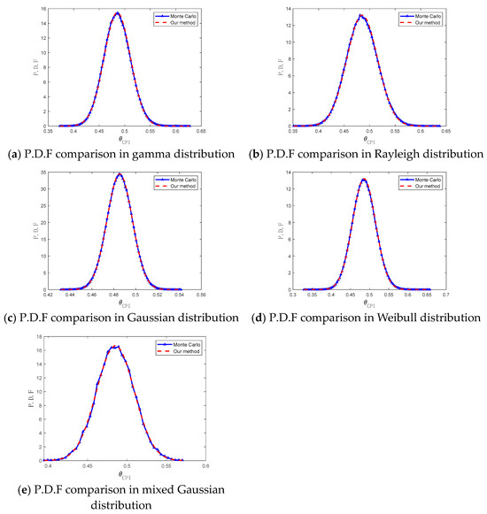
Figure 4.
P.D.F comparison between the Monte Carlo simulation and angle expansion model in uniformly accelerated linear motion scenario.
Table 4.
KS distance of the Monte Carlo simulation statistics and angle spread model in uniformly accelerated linear motion scenario.
5.2. The Angle Measurement Accuracy of the Angle Correction Algorithm
To validate the angle measurement performance of the multi-pulse integration and long-term estimation angle correction algorithm proposed in this chapter under low signal-to-noise ratio (SNR) conditions, additional noise of varying intensities was introduced into the simulation experiments described in Section 5.1.1 and Section 5.1.2, altering the target SNR from 0 dB to 20 dB. The traditional monopulse amplitude comparison angle measurement method and the proposed multi-pulse long-term estimation algorithm were then applied to the target echo data to obtain angle measurement results. For each SNR, 1000 Monte Carlo simulations were conducted to calculate the root mean square error (RMSE) between the angle measurement results and the true angle values for both methods.
Figure 5 shows the variation in RMSE of angle error with SNR for both the traditional monopulse angle measurement algorithm and the multi-pulse integration and long-term estimation algorithm in uniform linear motion and uniformly accelerated linear motion scenarios. It can be seen that as the SNR increases, the RMSE of both algorithms decreases, and under high SNR conditions, the RMSEs of the two algorithms converge. However, under low SNR conditions, the performance of the multi-pulse integration and long-term estimation algorithm is significantly better than that of the traditional monopulse angle measurement algorithm. In the uniform linear motion scenario, when the SNR is 0 dB, the RMSE of the traditional monopulse angle measurement is 0.29, while the RMSE of the multi-pulse integration and long-term estimation algorithm is only 0.08. In the uniformly accelerated linear motion scenario, under 0 dB SNR conditions, the RMSE of the traditional monopulse angle measurement is 0.33, while the RMSE of the multi-pulse integration and long-term estimation algorithm is only 0.10. Theoretically, the error of traditional monopulse angle measurement is consistent under uniform velocity and uniform acceleration scenarios. However, in the simulation, the error under uniform acceleration is greater than under uniform velocity at the same signal-to-noise ratio. This is because the radar in the simulation of the Ku-band high-resolution phased array radar employs stepped frequency wideband synthesis, combining ten 125 MHz sub-band signals into a single 1 GHz wideband range profile (as shown in Table 1), followed by monopulse angle measurement. Stepped frequency synthesis is equivalent to a coherent integration. During these ten sub-pulses, the motion of the target causes divergence in the range profile, which is more pronounced under uniform acceleration. Additionally, the target’s angle changes between the sub-pulses, with more dramatic variations under uniform acceleration. Therefore, the error in traditional monopulse angle measurement is larger in the uniform acceleration case.
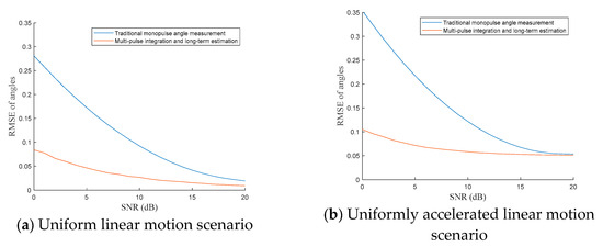
Figure 5.
Angular error RMSE of the two angular measurement algorithms varies with the SNR under different motion scenarios for the Ku-band high-resolution phased array radar.
In order to eliminate the influence of step-frequency signal synthesis on the angle measurement, we set other S-band low-resolution radar system parameters as the simulation parameters. Different from the Ku-band high-resolution phased array radar, it transmits linear frequency modulation signals with a carrier center frequency of 3 GHz and a bandwidth of 20 MHz. It can generate a one-dimensional range image without sub-pulse synthesis. The system parameters of the S-band simulation are shown in Table 5, and the other simulation parameters are consistent with the parameters of the Ku-band high-resolution phased array radar in Table 1. The signal-to-noise ratio of the target is changed from 0 dB to 20 dB. For each signal-to-noise ratio, the RMSE of the angle measurement is statistically calculated after 1000 Monte Carlo simulations. The results are shown in Figure 6, where the RMSE of the traditional single-pulse angle measurement remains consistent under uniform linear motion and uniformly accelerated linear motion scenarios but is higher than the algorithm proposed in this paper. Under low signal-to-noise ratio conditions, the RMSE of the algorithm proposed in this paper is much lower than the RMSE of the traditional algorithm, which means that the angle measurement accuracy performance advantage of the algorithm proposed in this paper is more obvious under a low signal-to-noise ratio. This is because the multi-pulse integration improves the signal-to-noise ratio, and the angle measurement is less affected by noise. At the same time, the angle expansion model compensates for the errors caused by target amplitude fluctuations and movement. Therefore, under a low signal-to-noise ratio, the angle measurement accuracy of the algorithm proposed in this paper is better than that of the traditional method.
Table 5.
Simulation radar system parameters under S-band radar.
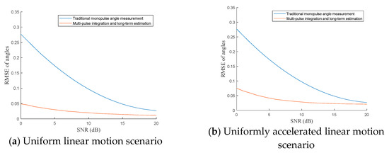
Figure 6.
Angular error RMSE of the two angular measurement algorithms varies with the SNR under different motion scenarios for S-band low-resolution radar.
6. Verification with Measured Data
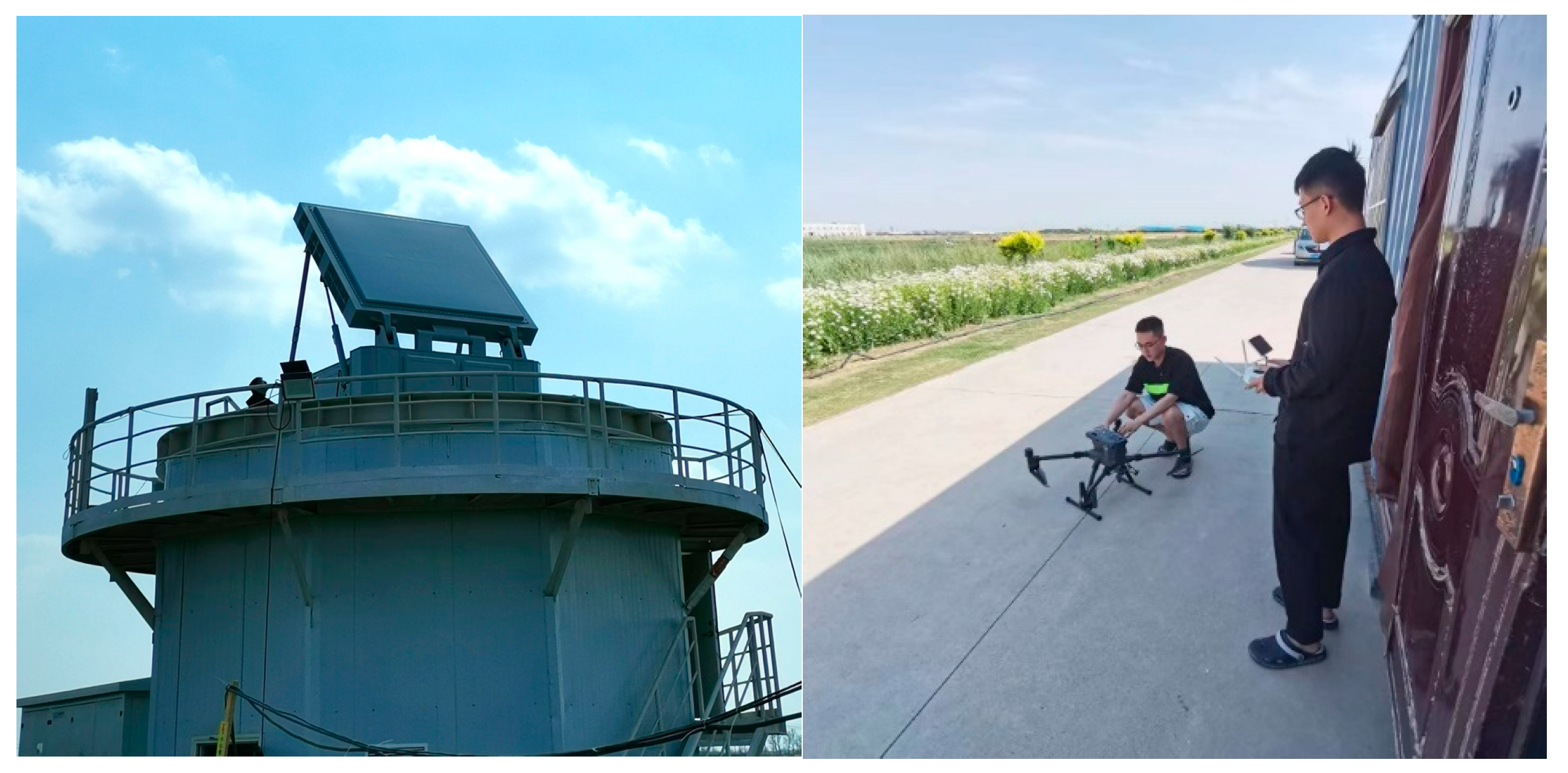
To verify the application performance of the multi-pulse integration and long-term estimation angle correction algorithm in practical radar angle measurement, as shown in Figure 7, this paper uses data collected from a Ku-band high-resolution phased array radar equipped with high-precision RTK-guided unmanned aerial vehicle (UAV). The system parameters of the high-resolution phased array radar are listed in Table 1, Section 5.1, while the UAV model parameters and flight motion parameters are provided in Table 6.

Figure 7.
Ku-band high resolution phased array radar and high-precision RTK UAV for take-off.
Table 6.
Model parameters and flight motion parameters of UAV.
As shown in Table 6, the RTK positioning accuracy of the DJI M300 can reach centimeter-level precision, which is extremely high. Therefore, the angle measured by the DJI RTK relative to the radar can be considered as the true value. Low-altitude UAV data flying radially along the radar line of sight was collected, and the multi-frame one-dimensional range profiles of the UAV radar echo signals in two scenarios are shown in Figure 8. For experimental convenience, it was necessary for the UAV to stay within the beam width for an extended period. Therefore, the UAV pilot controlled the UAV to fly horizontally along the radar line of sight, with the azimuth angle remaining almost unchanged while the elevation angle varied with the distance. As a result, the precision analysis in the azimuth dimension is not significant, and the angle measurement accuracy is analyzed and compared between the traditional monopulse angle measurement algorithm and the multi-pulse integration and long-term estimation angle correction algorithm proposed in this chapter, focusing only on the elevation angle.
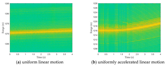
Figure 8.
Multi-frame radar one-dimensional range profile of UAV echo under uniform linear motion and uniformly accelerated linear motion.
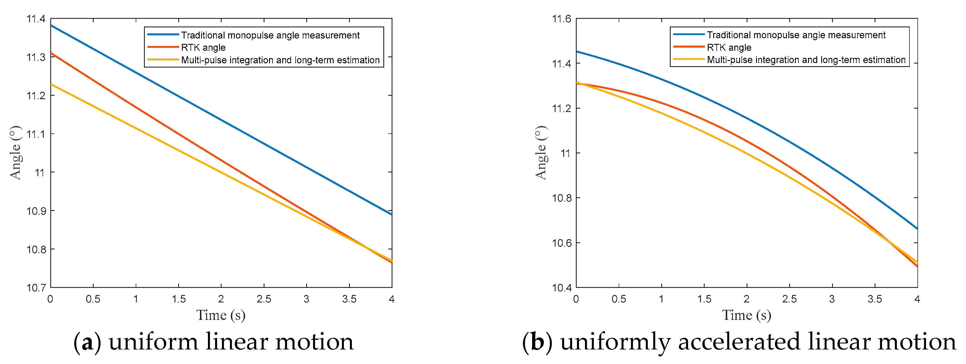
Figure 9 shows the pitch angles measured by RTK and the angle estimates from the two algorithms under the two motion scenarios. Using RTK angles as the true values, the RMSE for the multi-pulse integration and long-term time estimation angle correction algorithm was 0.04 in the uniform linear motion scenario and 0.07 in the uniformly accelerated linear motion scenario, while the traditional single-pulse angle measurement algorithm had RMSE values of 0.09 and 0.11, respectively. This indicates that the multi-pulse integration and long-term time estimation angle correction algorithm outperforms the traditional single-pulse angle measurement algorithm in both uniform linear and uniformly accelerated linear motion scenarios, confirming its applicability in real-world situations.
Figure 9.
Pitch angles from RTK and two angle estimation algorithms in uniform linear and uniformly accelerated linear motion scenarios.
7. Conclusions
To address the issue of low signal-to-noise ratio (SNR) and significant noise-reducing single-pulse angle measurement accuracy for small aerial targets, we proposed an angle estimation algorithm based on multi-pulse integration. Given the insufficient research and analysis on multi-pulse integration angle measurement, we constructed an angle measurement model under multi-pulse coherent integration based on the single-pulse measurement principle and target motion model. Unlike traditional assumptions based on single-pulse measurements, during multi-pulse integration, the target’s displacement and amplitude fluctuations lead to angle measurement expansion. Therefore, we developed angle extension models for both uniform linear motion and uniformly accelerated linear motion scenarios based on the Lindeberg–Feller central limit theorem. Our analysis revealed that when the number of pulses is sufficiently large, the multi-pulse measurement error due to target motion and amplitude fluctuations approaches a Gaussian distribution. The mean and variance of the Gaussian distribution are related to target motion parameters and amplitude fluctuation distributions, with detailed derivations provided.
Finally, based on the angle extension models for both motion scenarios, we proposed an angle correction algorithm based on multi-pulse integration and long-term estimation. Simulation experiments demonstrated the accuracy of the Gaussian approximation angle extension model. Compared to traditional single-pulse measurement algorithms, the proposed multi-angle correction method can reduce accuracy estimation errors by up to 67% under 0 dB SNR conditions. Comparison with RTK data collected from UAVs in field tests shows that the proposed multi-pulse angle measurement algorithm provides higher measurement accuracy, further validating its effectiveness in practical applications.
Author Contributions
Methodology, J.C.; Validation, J.C. and H.Y.; Formal analysis, R.W.; Resources, H.Y.; Data curation, H.Y.; Writing—original draft, J.C.; Writing—review & editing, R.W.; Funding acquisition, R.W. All authors have read and agreed to the published version of the manuscript.
Funding
This work was supported by the National Natural Science Foundation of China under Grant 31727901.
Data Availability Statement
The data presented in this study are available on request from the author. The data are not publicly available because it is currently privileged information.
Conflicts of Interest
The authors declare no conflict of interest.
Appendix A
Assuming that the probability density function of is , can be rewritten as:
Let , then
and with the implicit condition .
We first prove that is symmetric about , that is:
Let be the cumulative distribution function of , that is, . We will now prove that .
Using , we can perform an equivalent transformation on the inequality , resulting in:
Assuming
is any value that satisfies the condition .
Then,
must be a value that satisfies , and vice versa.
Additionally, since are independently and identically distributed, the order of the values taken by is equivalent, that is:
Therefore,
which proves that .
The expectation of can be transformed as follows:
for , let . Using Equation (A3), we obtain:
Therefore,
By symmetry and the properties of the probability density function, we obtain:
This proves that
References
- Xiong, X.; Deng, Z.; Qi, W.; Dou, Y. High-precision angle estimation based on phase ambiguity resolution for high resolution radars. Sci. China Inf. Sci. 2019, 62, 040307. [Google Scholar] [CrossRef]
- Zheng, Y.; Chen, B. Altitude measurement of low-angle target in complex terrain for very high-frequency radar. IET Radar Sonar Navig. 2015, 9, 967–973. [Google Scholar] [CrossRef]
- Joshi, S.K.; Baumgartner, S.V.; da Silva, A.B.C.; Krieger, G. Direction-of-arrival angle and position estimation for extended targets using multichannel airborne radar data. IEEE Geosci. Remote Sens. Lett. 2022, 19, 4022705. [Google Scholar] [CrossRef]
- Okay, F.Y.; Özdemir, S. Real-time Aircraft Tracking System: A Survey and A Deep Learning Based Model. In Proceedings of the 2021 International Symposium on Networks, Computers and Communications (ISNCC), Dubai, United Arab Emirates, 31 October–2 November 2021; IEEE: Piscataway, NJ, USA, 2021; pp. 1–6. [Google Scholar]
- Lo, K. Theoretical analysis of the sequential lobing technique. IEEE Trans. Aerosp. Electron. Syst. 1999, 35, 282–293. [Google Scholar] [CrossRef]
- Lank, G.; Pollon, G. Exact Angular Accuracy of an Amplitude Comparison Sequential-Lobing Processor. IEEE Trans. Aerosp. Electron. Syst. 1974, AES-10, 393–398. [Google Scholar] [CrossRef]
- Kirkpatrick, G. Development of A Monopulse Radar System. IEEE Trans. Aerosp. Electron. Syst. 2009, 45, 807–818. [Google Scholar] [CrossRef]
- Leonov, A. History of monopulse radar in the USSR. IEEE Aerosp. Electron. Syst. Mag. 1998, 13, 7–13. [Google Scholar] [CrossRef]
- Sinsky, A.; Lew, E. Comparative analysis of a phase and an amplitude processor for amplitude monopulse systems. IEEE Trans. Antennas Propag. 1983, 31, 519–522. [Google Scholar] [CrossRef]
- Sebt, M.; Goodarzi, M.; Darvishi, H. Geometric Arithmetic Mean Method for Low Altitude Target Elevation Angle Tracking. IEEE Trans. Aerosp. Electron. Syst. 2023, 59, 5111–5119. [Google Scholar] [CrossRef]
- Darvishi, H.; Sebt, M. Adaptive hybrid method for low-angle target tracking in multipath. IET Radar Sonar Navig. 2018, 12, 931–937. [Google Scholar] [CrossRef]
- Park, D.; Yang, E.; Ahn, S.; Chun, J. Adaptive beamforming for low-angle target tracking under multipath interference. IEEE Trans. Aerosp. Electron. Syst. 2014, 50, 2564–2577. [Google Scholar] [CrossRef]
- Xu, Z.; Xiong, Z.; Wu, J.; Xiao, S. Symmetrical difference pattern monopulse for low-angle tracking with array radar. IEEE Trans. Aerosp. Electron. Syst. 2016, 52, 2676–2684. [Google Scholar] [CrossRef]
- Seifer, A. Monopulse-radar angle tracking in noise or noise jamming. IEEE Trans. Aerosp. Electron. Syst. 1992, 28, 622–638. [Google Scholar] [CrossRef]
- Han, H.; Xu, X.; Wang, H.; Dai, H. Analysis of Cross-polarization Jamming for Phase Comparison Monopulse Radars. In Proceedings of the 2019 IEEE 2nd International Conference on Electronic Information and Communication Technology (ICEICT), Harbin, China, 20–22 January 2019; pp. 404–407. [Google Scholar]
- Chen, X.; Shu, T.; Yu, K.; Yu, W. Enhanced ADBF Architecture for Monopulse Angle Estimation in Multiple Jammings. IEEE Antennas Wirel. Propag. Lett. 2017, 16, 2684–2687. [Google Scholar] [CrossRef]
- Yu, K.; Murrow, D. Adaptive digital beamforming for angle estimation in jamming. IEEE Trans. Aerosp. Electron. Syst. 2001, 37, 508–523. [Google Scholar]
- Gogineni, S.; Nehorai, A. Monopulse MIMO Radar for Target Tracking. IEEE Trans. Aerosp. Electron. Syst. 2011, 47, 755–768. [Google Scholar] [CrossRef]
- Zhang, X.; Willett, P.; Bar-Shalom, Y. Detection and Localization of Multiple Unresolved Extended Targets via Monopulse Radar Signal Processing. IEEE Trans. Aerosp. Electron. Syst. 2009, 45, 455–472. [Google Scholar] [CrossRef]
- Fu, M.; Gao, C.; Li, Y.; Deng, Z.; Chen, D. Monopulse-Radar Angle Estimation of Multiple Targets Using Multiple Observations. IEEE Trans. Aerosp. Electron. Syst. 2021, 57, 968–983. [Google Scholar] [CrossRef]
- Huang, Q.; Fan, H.; Cai, F.; Xiao, H. Joint Estimation of Unresolved Leader–Follower in the Presence of Dense False Signals Using Monopulse Radar. IEEE Trans. Aerosp. Electron. Syst. 2023, 59, 9635–9649. [Google Scholar] [CrossRef]
- Palamà, R.; Fioranelli, F.; Ritchie, M.; Inggs, M.; Lewis, S.; Griffiths, H. Measurements and discrimination of drones and birds with a multi-frequency multistatic radar system. IET Radar Sonar Navig. 2021, 15, 841–852. [Google Scholar] [CrossRef]
- Wang, R.; Cai, J.; Hu, C.; Zhou, C.; Zhang, T. A Novel Radar Detection Method for Sensing Tiny and Maneuvering Insect Migrants. Remote Sens. 2020, 12, 3238. [Google Scholar] [CrossRef]
- Wang, R.; Zhang, T.; Hu, C.; Cai, J.; Li, W. Digital detection and tracking of tiny migratory insects using vertical-looking radar and ascent and descent rate observation. IEEE Trans. Geosci. Remote Sens. 2021, 60, 5101615. [Google Scholar] [CrossRef]
- Wang, J.; Guo, P.; Lei, P.; Wei, S. Influence and compensation of target motion on monopulse estimation in PD radar. In Proceedings of the IEEE 10th International Conference on Signal Processing, Beijing, China, 24–28 October 2010; IEEE: Piscataway, NJ, USA, 2010; pp. 2312–2315. [Google Scholar]
- Medina, P.K.; Merino, S.; Galton, F. The Central Limit Theorem. In Mathematical Finance and Probability: A Discrete Introduction; Springer: Berlin/Heidelberg, Germany, 2003; pp. 221–246. [Google Scholar]
- Chow, Y.S.; Teicher, H.; Chow, Y.S.; Teicher, H. Central limit theorems. Probab. Theory Indep. Interchang. Martingales 1988, 295–335. [Google Scholar]
- Rio, E. About the Lindeberg method for strongly mixing sequences. ESAIM Probab. Stat. 1997, 1, 35–61. [Google Scholar] [CrossRef]
- Klenke, A.; Klenke, A. Characteristic Functions and the Central Limit Theorem. Probab. Theory A Compr. Course 2020, 327–366. [Google Scholar]
- Adachi, A.; Kobayashi, T.; Yamauchi, H. A Methodology for Estimating the Parameters of a Gamma Raindrop Size Distribution Model from Polarimetric Radar Measurements at Attenuating Frequency Based on the Self-Consistency Principle. In Proceedings of the EGU General Assembly Conference Abstracts, Vienna, Austria, 17–22 April 2016; p. EPSC2016-5381. [Google Scholar]
- Blair, W.D.; Brandt-Pearce, M. Monopulse DOA estimation of two unresolved Rayleigh targets. IEEE Trans. Aerosp. Electron. Syst. 2001, 37, 452–469. [Google Scholar] [CrossRef]
- Ehrman, L.M.; Blair, W.D. Using target RCS when tracking multiple Rayleigh targets. IEEE Trans. Aerosp. Electron. Syst. 2010, 46, 701–716. [Google Scholar] [CrossRef]
- Buller, W.; Wilson, B.; van Nieuwstadt, L.; Ebling, J. Statistical modelling of measured automotive radar reflections. In Proceedings of the 2013 IEEE International Instrumentation and Measurement Technology Conference (I2MTC), Minneapolis, MN, USA, 6–9 May 2013; IEEE: Piscataway, NJ, USA, 2013; pp. 349–352. [Google Scholar]
- Zhang, Y.; Shen, J.; Tuo, X.; Yang, H.; Zhang, Y.; Huang, Y. Scanning radar forward-looking superresolution imaging based on the Weibull distribution for a sea-surface target. IEEE Trans. Geosci. Remote Sens. 2022, 60, 5116111. [Google Scholar] [CrossRef]
- Pierce, R.D. RCS characterization using the alpha-stable distribution. In Proceedings of the Proceedings of the 1996 IEEE National Radar Conference, Ann Arbor, MI, USA, 13–16 May 1996; IEEE: Piscataway, NJ, USA, 1996; pp. 154–159. [Google Scholar]
- Seybold, J.S.; Weeks, K.L. Arithmetic versus geometric mean of target radar cross section. Microw. Opt. Technol. Lett. 1996, 11, 265–270. [Google Scholar] [CrossRef]
- Wang, L.; Xie, G.; Qian, F.; Jin, Y.; Gao, K. A novel model for analyzing the statistical properties of targets’ RCS. IEEE Signal Process. Lett. 2021, 29, 583–586. [Google Scholar] [CrossRef]
- Massey, F.J., Jr. The Kolmogorov-Smirnov test for goodness of fit. J. Am. Stat. Assoc. 1951, 46, 68–78. [Google Scholar] [CrossRef]
- Xia, X.; Shui, P.; Zhang, Y.; Li, X.; Xu, X. An empirical model of shape parameter of sea clutter based on X-band island-based radar database. IEEE Geosci. Remote Sens. Lett. 2023, 20, 3503205. [Google Scholar] [CrossRef]

Disclaimer/Publisher’s Note: The statements, opinions and data contained in all publications are solely those of the individual author(s) and contributor(s) and not of MDPI and/or the editor(s). MDPI and/or the editor(s) disclaim responsibility for any injury to people or property resulting from any ideas, methods, instructions or products referred to in the content. |
© 2024 by the authors. Licensee MDPI, Basel, Switzerland. This article is an open access article distributed under the terms and conditions of the Creative Commons Attribution (CC BY) license (https://creativecommons.org/licenses/by/4.0/).