3D Reconstruction of Building Blocks Based on Extraction of Exterior Wall Lines Using Point Cloud Density Generated from Spherical Camera Images

Abstract

The 3D modeling of urban buildings has become a common research area in various disciplines such as photogrammetry and computer vision, with different applications such as intelligent city management, navigation of self-driving cars and architecture, just to name a few. The objective of this study is to produce a 3D model of the external facade of the buildings with the required precision, accuracy and level of detail according to the user’s requirements, while minimizing time and cost. This research focuses on the production of 3D models for blocks of residential buildings in Tehran, Iran. The Insta 360 One X2 spherical camera is selected to capture the data due to its low cost and 360 × 180° field of view. The camera specifications have facilitated more efficient data collection in terms of both time and cost. The proposed modeling method is based on extracting lines of external walls through the utilization of the point cloud density concept. Initially, photogrammetric point clouds are generated in with a reconstruction precision of 0.24 m from spherical camera images. In the next step, the 3D point cloud is projected into a 2D point cloud by setting the height component to zero. The 2D point cloud is then rotated based on the direction angle determined by the Hough transform so that the perpendicular walls are parallel to the axes of the coordinate system. Next, a 2D point cloud density analysis is performed by voxelizing the point cloud and counting the number of points in each voxel in both the horizontal and vertical directions. By determining the peaks in the density plot, the lines of the external vertical and horizontal walls are extracted. To extract the diagonal external walls, the density analysis is performed in the direction of the first principal component. Finally, by determining the height of each wall in the point cloud, a 3D model is created at the level of detail one. The resulting model has a precision of 0.32 m compared to real sizes, and the 2D plan has a precision of 0.31 m compared to the ground truth map. The use of the spherical camera and point cloud density analysis makes this method efficient and cost-effective, making it a promising approach for future urban modeling projects.

1. Introduction

The 2D plans and 3D models of urban building blocks are important in various applications such as intelligent city management, cadastre and taxation, navigation of robots and self-driving cars, architecture and also the tourism industry.

The 3D modeling of buildings at large urban scales is often carried out using photogrammetry and remote sensing data such as satellite imagery [1], aerial photogrammetry using aircraft [2], drone [3] and also mobile mapping systems [4].

Considering that aerial and satellite platforms can cover large areas such as cities, but with problems such as the high cost of flying, modeling complex roofs, hiding walls under roofs and also hiding shorter walls such as courtyard walls under trees mean that the building area may not be correctly extracted. In addition, because of the need to create models of building facades and the insufficient visibility provided by aerial and satellite platforms, the use of UAVs and MMS is being explored to offer multi-view imaging capabilities on city streets, which are often obstructed by structures.

Among the common sensors used in the production of 3D models based on the image, there are perspective cameras with a limited field of view. Considering that the length of the streets is much more than their width and the streets are limited by structures, using perspective cameras is not a good choice. Currently, spherical cameras with a field of view of 360 × 180° can capture the entire surrounding environment in a single image, making it possible to cover large urban areas. Also, their low cost has increased their popularity. Spherical cameras have been used in various modeling applications over the last two decades, such as building interior modelling [5], building exterior and façade modeling [6], cultural heritage modeling [7,8], the 3D reconstruction of tunnels [9] and gas and water pipelines [10,11].

A variety of methods have been presented to produce a 3D model, all of which are a subset of the four general methods of data-driven modelling, model-driven, grammar-based and machine learning. Different techniques have been presented at different levels of automation, but most of the methods used are in the data-driven modeling group. In the data-driven method, the 3D reconstruction is performed in such a way that the basic elements, which are often simple geometric shapes, are reconstructed and then the topological relationships between them are defined. This modeling method is proposed for high-density point clouds without gaps, occluded areas and noise. As a result, researchers are always looking for solutions to deal with noise, gaps, occluded areas and low density in data-driven modeling.

An example of building modeling using a data-driven method is to separate the roof, floor and wall slabs, define the topological relationships between them and create a 3D model. For instance, one study proposed an automated framework that segments planar surfaces and applies contextual reasoning based on height, orientation and point density to classify elements such as floors and walls from point cloud data [12]. Another study introduced a semi-automatic method for interior 3D reconstruction. This method segments walls, ceilings, and floors from point clouds and reconstructs them in the Industry Foundation Classes (IFCs) format for integration into building information models (BIMs) [13]. Additionally, a fully automated method was developed using integer linear optimization to segment rooms, remove outliers and generate interconnected volumetric walls [14]. In addition, the method involves separating the floor and ceiling, followed by segmentation and computation of α-shapes to construct an adjacency graph for intersecting planes. Using a boundary representation (B-rep) approach, an initial 3D model is created, which is then refined by analyzing the adjacency graph of the intersected planes, resulting in a water-tight and topologically correct model [15].

Another data-driven 3D modeling method that is faster and easier than the other methods is to extract the footprint of the building and then elevate it to create a 3D model. One such method comprises three steps, as follows: the identification of boundary edges, the tracing of a sequence of points, and the generation of final lines. This method is effective in managing challenges such as the detection of concave shapes and holes, while providing high accuracy even with low-density data [16,17]. Another study examined the influence of point cloud density on the quality of extracted outlines, comparing two approaches (direct extraction and raster method) and emphasizing the significance of data quality in footprint generation [18]. Furthermore, a pipeline combining non-parametric kernel density estimation (KDE) and the traveling Salesperson salesperson problem (TSP) was employed for 2D footprint extraction, resulting in enhanced overall footprint geometry through the application of clustering techniques such as DBSCAN [19]. Other methods entail the filtration, segmentation and regularization of building boundaries derived from LiDAR points, whereby the precision of the regularized boundary is found to be directly proportional to the point cloud density [20]. Moreover, an indoor plane extraction method utilizing an optimized RANSAC algorithm and space decomposition exhibited enhanced performance in the detection of building components in occluded interior spaces, when compared to the traditional method [21]. Consequently, various techniques for extracting the building footprint from the point cloud are being developed with the objective of enhancing the accuracy and efficiency of the process, thereby extending its applicability to low-density point cloud data.

The basic data modeling techniques mentioned above include separating ceiling, floor and wall panels from the point cloud and defining their topological and geometric relationships. In some research, researchers have used this modelling method and extracted wall lines from the separated wall panels and then elevated these lines to obtain a 3D model of the building [22,23].

Many line extraction approaches using classical methods such as the Hough transformation are not suitable for complex buildings due to lack of flexibility, and the proposed approaches based on this type of transformation have been generalized or used together with other algorithms. For example, the Hough transform is a prevalent voting scheme for the detection of lines in 3D point clouds, which employs a regularization technique to enhance parameter quantization. The iterative process identifies the line with the greatest number of votes and applies orthogonal least squares fitting to enhance estimation accuracy [24]. A study on the utilization of terrestrial laser scanning from a mobile mappingsystem (MMS) in the context of building footprints, demonstrates the efficacy of this approach in urban environments. The integration of the Hough transforms with k-means clustering and RANSAC enables the precise extraction of building footprints from raw 3D data [25]. Furthermore, the orderedpoints–aided Hough transform(OHT) employs ordered edge points to extract high-quality building outlines from airborne LiDAR data, achieving high completeness (90.1% to 96.4%) and correctness (over 96%), while demonstrating superior positional accuracy and performance on complex datasets [26].

Another suggestion for extracting building footprints is to use several types of data together, such as the combination of aerial photogrammetry data and ground laser scanners, which increases the accuracy and efficiency in data-driven modeling [27,28].

Therefore, it is important to provide a method that can extract the wall lines and convert them into a 3D model despite the gap, noise and low density in the point cloud, that is simple and fast, and that is also compatible with the different geometric shapes of the buildings.

The method introduced in this research is based on the analysis of the density of the point cloud generated from the images of the spherical camera to extract the lines of the external walls. The main hypothesis is that according to the definition of density in a 2D point cloud, it is the number of points per unit area, and in a 3D point cloud, it is the number of points per unit volume. With the assumption that the intersection of the walls always has a higher density than the surface of the walls, by changing the viewing angle in relation to the point in the horizontal direction, the vertical walls are displayed with more density, and also by changing the viewing angle in the vertical direction, the horizontal walls are displayed with more density. Therefore, this method covers one of the problems of data-driven modeling, which is low density, by changing the viewing angle relative to the point cloud.

The aim of this research is the 3D reconstruction of building blocks as the main urban elements in a residential area in Tehran with optimal precision and accuracy at the level of detail one by solving the challenges of using Insta360 One X2 spherical camera images on an urban scale and using density analysis and principal component analysis in extracting the lines of the external walls from the point cloud of the building block to reach a 2D plan (LOD0) and the next step is to elevate the wall lines based on the point cloud and produce a 3D model at the level of detail one (LOD1).

The rest of this article is organized as follows: Section 2 reviews and explains the network design and data collection, point cloud generation in Agisoft Metashape (Company: Agisoft Metashape, version 2.0.2), and density analysis. Section 3 shows the 3D model, prismatic model and 2D plan generated from the four building blocks obtained from the density analysis algorithm. The accuracy of the generated model is also evaluated. Section 4 presents a summary of the research, results and future suggestions.

2. Materials and Methods

In this section, a detailed explanation is provided of the various stages involved in the production of a 2D plan and 3D model, with a particular focus on the equirectangular images of the Insta 360 One X2 spherical camera. Section 2.1 covers the topics of sensor selection and data collection. In Section 2.2, the generation of a point cloud from equirectangular images in Metashape software 2.0.2 is discussed. The settings made and the output of different steps in order to generate a point cloud of four building blocks are presented. Finally, Section 2.3 introduces the algorithm of density analysis which is used to extract the lines of the external walls of the block.

2.1. Sensor Selection and Data Acquisition

Acquiring data from blocks of urban buildings requires the selection of a sensor that covers the area with the least number of images and the short data acquisition time, due to the large scale and the limitations of data acquisition due to the passage of people and vehicles in ground surveys. The spherical camera is chosen because it has 360 × 180° and can capture the entire environment in a single shot. Also, it is a low-cost sensor.

In general, spherical cameras, which are called polydioptric, are a subset of omnidirectional sensors. Polydioptric cameras are structurally composed of multiple shaped lenses that overlap to provide a field of view of 360 degrees in the horizontal plane and more than 180 degrees in the vertical plane [8,29].

Spherical cameras are available in both professional and consumer grade groups. Professional cameras are distinguished by a greater number of lenses, a higher weight, and a higher resolution, as well as a higher price point than consumer grade cameras [30].

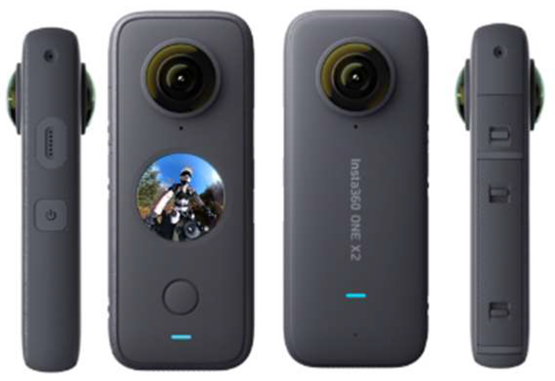
The employed camera in this research, Insta360 One X2 in Figure 1, is a consumer-grade camera. It consists of two fisheye lenses mounted back-to-back, giving a 360 × 180° field of view, a resolution of 6080 × 3040 pixel and a weight of 140 grams. This captures the entire environment around the camera in a single shot, creating a 3D model with fewer images and in less time. The reasons for choosing this camera among various types of consumer-grade spherical cameras are the low price, light weight, high resolution and higher quality image production in equirectangular projection than the Samsung and Ricoh spherical camera images.

The image produced by this camera (Figure 2a) is an equirectangular projection. In fact, two circular images of fisheye lenses are mapped onto one screen (Figure 2b), which is performedby the camera itself in three steps [31], as follows:

• Corresponding points on the boundary of the circular images of the fisheye lenses are extracted.
• The existing radial and tangential distortions are partially corrected.
• The circular image of the front lens is placed in the center of the screen, and the circular image of the rear lens is added to it from the sides.

The two circular images of the front and rear fisheye lens of the Insta 360 One X2 camera are raw images, these images are used to create a panoramic image of the equirectangular type using commercial camera software (Insta 360 studio one 2023), during this process the software performs the calibration process and adjusts the calibration parameters. Due to the commercial nature of this software, no information is available on how it works.

Tangential radial distortion caused by equirectangular mapping is one of the disadvantages of the Insta 360 One X2 camera.

Radial and tangential distortion lead to the 3D modeling process being unable to use algorithms based on perspective images when identifying key points and defining descriptors for feature detection and matching. For this reason, research has been carried out to solve this problem [32,33], and also commercial software such as Agisoft Metashape, Open MVG and Pix 4D Mapper have been developed to support equirectangular images.

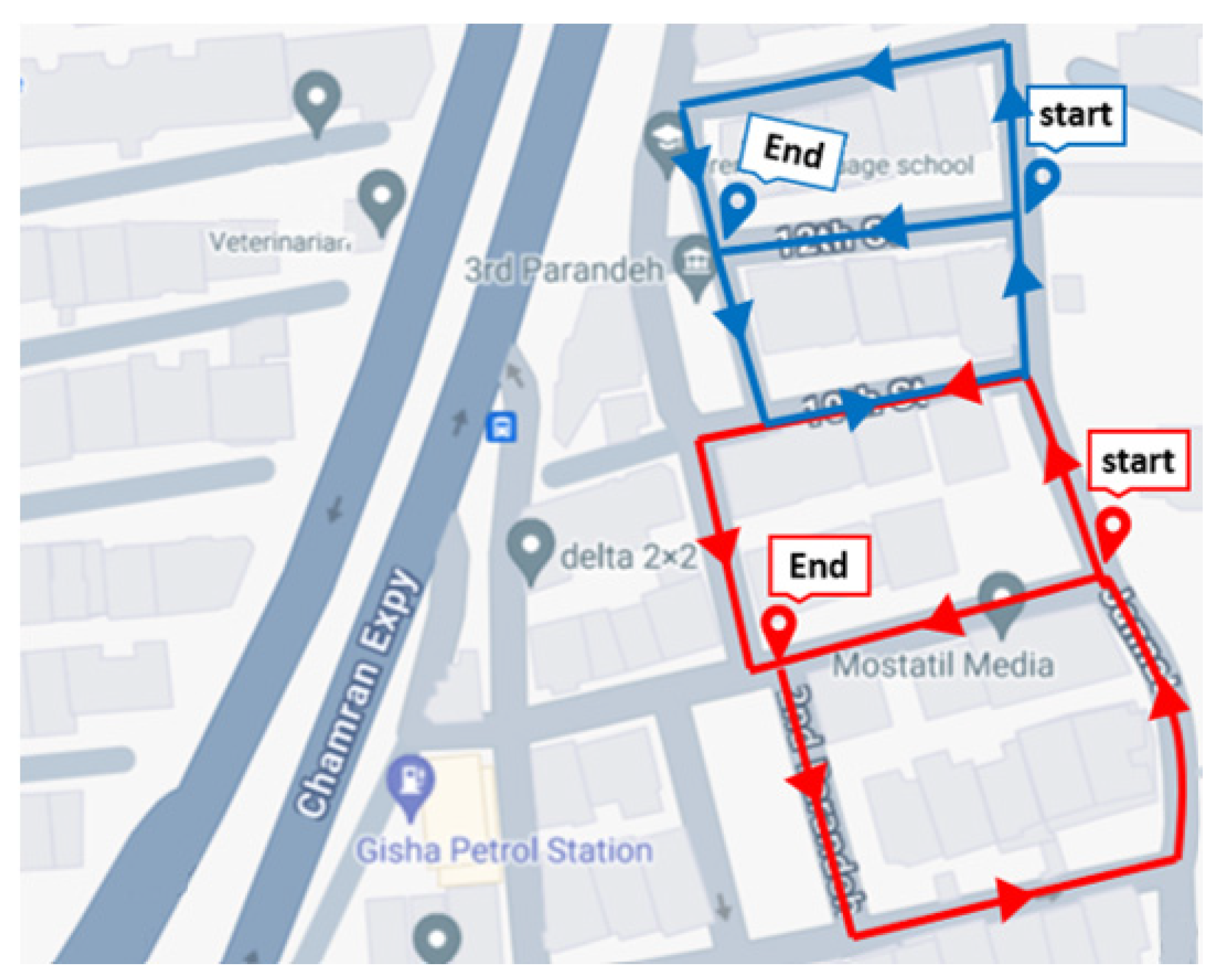
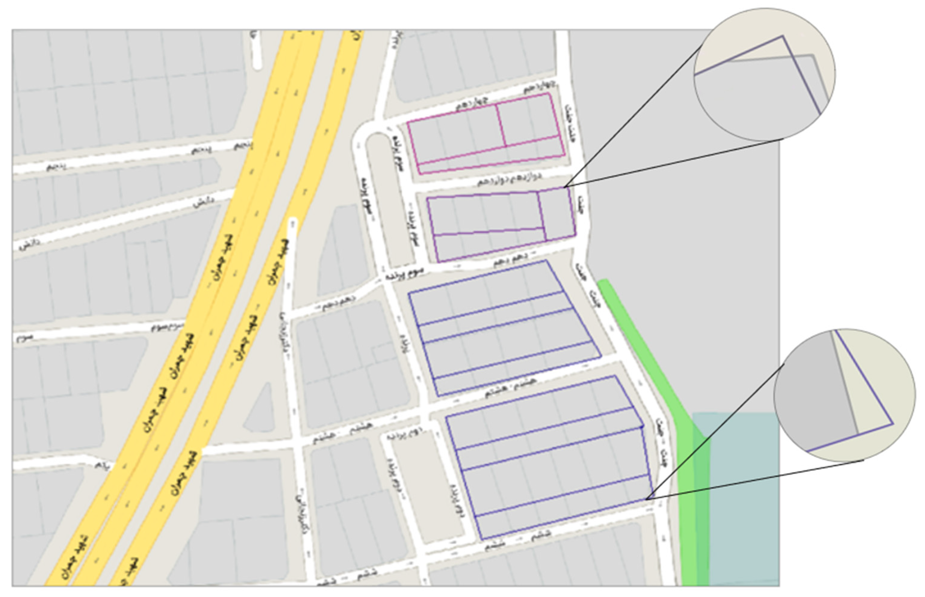
After selecting the appropriate sensor, it is necessary to collect the data and implement a suitable network design. When collecting data on urban roads with limited structures on both sides, the ideal network is a closed path with the same distance from structures on both sides of the road. This network is ideal because ground-based stations can have a sufficient view of the high structures on both sides of the road at the same time.

In the following article, the same network model has been implemented because the roads considered are residential and crossing the center line of the road is unimpeded. However, it is proposed to move back and forth from the lane next to the pedestrian crossing in the main streets where vehicles pass.

As a result, the network designed for this case study consists of two closed routes with stations along the center line of the road, as can be seen in Figure 3.

In the design of the network, three station distances were investigated, of 1, 2 and 3 m.

One meter station: The point cloud produced has the highest density and the highest accuracy, which means the lowest amount of reprojection error (1.06 pix) compared to two meters and three meters distance, Thecoverage of images with each other is 90%, and this high coverage of images, despite the fact that it leads to the point cloud, has been increased with density and has created higher accuracy. However, due to the use of a spherical camera, which is expected to perform modeling with a smaller number of images, it is in contradiction, and also a high number of images increases the time and cost of calculations, which according to the data obtained is not recommended on a large scale in the city.

Three-meter station: The point cloud produced has the lowest density and accuracy (highest reprojection error (1.984 pix)) compared to the distances of one meter and two meters, the coverage of the images is 60%, and because the road is extended in the longitudinal direction compared to the width, the lack of images has caused a gap in the point cloud.

Two-meter station: The point cloud produced has a lower density and accuracy (reprojection error = 1.28 pix) compared to the distance of one meter, but the difference in the amount of the reprojection errors is small (./22 pix), the coverage of 75% of the images has resulted in the production of a point cloud with uniform density and without gaps, and also when compared to the distance of one meter, this has been able to cover a large area and produce an optimal point cloud with a smaller number of images. These characteristics lead to the selection of two meters as the optimal stationing distance.

In addition to the images, the number of 36 scale bars (fixed distances), which are random measurements of the length, width and depth of the doors or windows of the buildings, were measured using a laser meter to increase the accuracy of the modelling, and finally, all the information related to data collection is mentioned in

Table 1. Information related to network design and data collection.

Data Acquisition Information	Values
Distance covered (m)	740
Number of images	355
Height of the camera above the ground (m)	2.68
Mean distance between the stations (m)	2
Number of horizontal and vertical scalebars	36

.

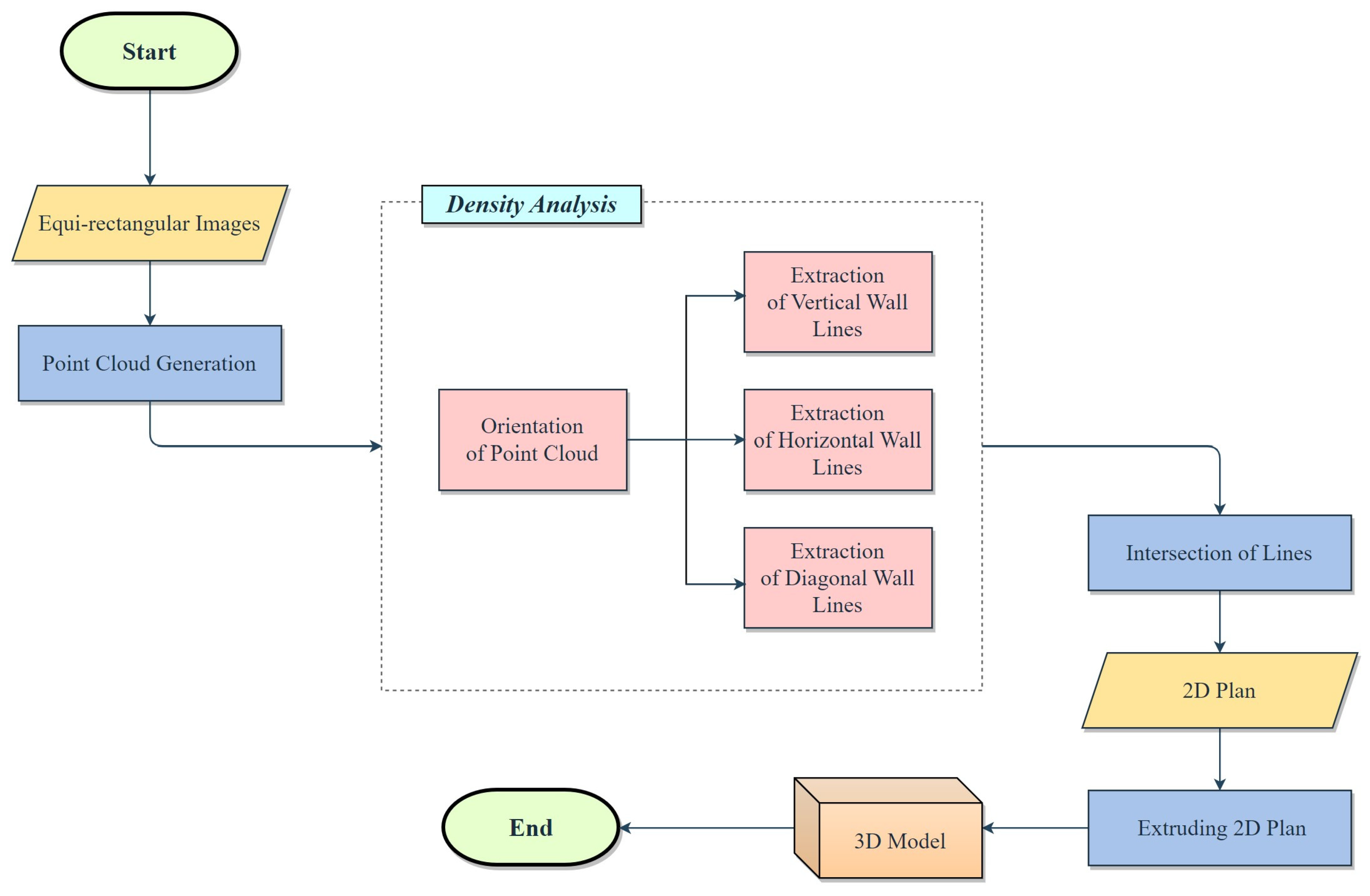
The following section explains the different stages of generating the 3D model of the building blocks from the equirectangular images collected according to the flowchart in Figure 4.

2.2. Pointcloud Generation

Agisoft Metashape software supports different image formats such as frame, fisheye, sphere in equirectangular projection and cylinder. Therefore, in this research, to process the images, this software wasused in the form of a sphere frame that supports equirectangular projection images. As previously stated, equirectangular images are generated from two raw circular images (two front and rear fisheye lenses) using commercial camera software (Insta 360 Studio 2023). During this process, the images are calibrated by the camera software and the pre-calibrated images are entered into the Metashape software. Consequently, the camera calibration parameters are disabled in Metashape software. Indeed, at this stage, a free bundle adjustment has been conducted; this refers to the process of bundle adjustment, which does not involve the calibration parameters, and the software is now solely responsible for the 3D reconstruction.

Table 2. Settings made in Agisoft Metashape 2.0.2 software to generate point cloud from Insta 360 One X2 spherical camera images.

Settings	Values
Type of images	Geotag, Map: ERP
Number of images	355
Quality of images	≥0.8
Coordinate system	UTM, zone 39N
Frame type	Spherical
Camera accuracy	10 m
Align settings of images	Level: Highest Reference preselection Threshold number of key points: 40,000 Threshold number of tie point: 4000
Scalebar accuracy	1 mm
Dense point cloud generation	Ultra-high
Reliability coefficient in classification	0.01

lists all the settings made in the Metashape software to generate a point cloud from the equirectangular images of the Insta 360 One X2 camera.

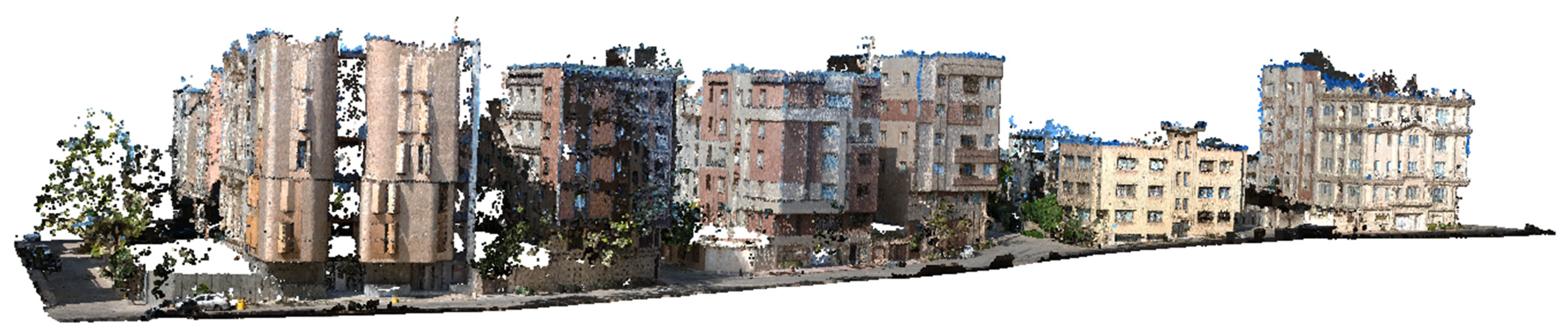
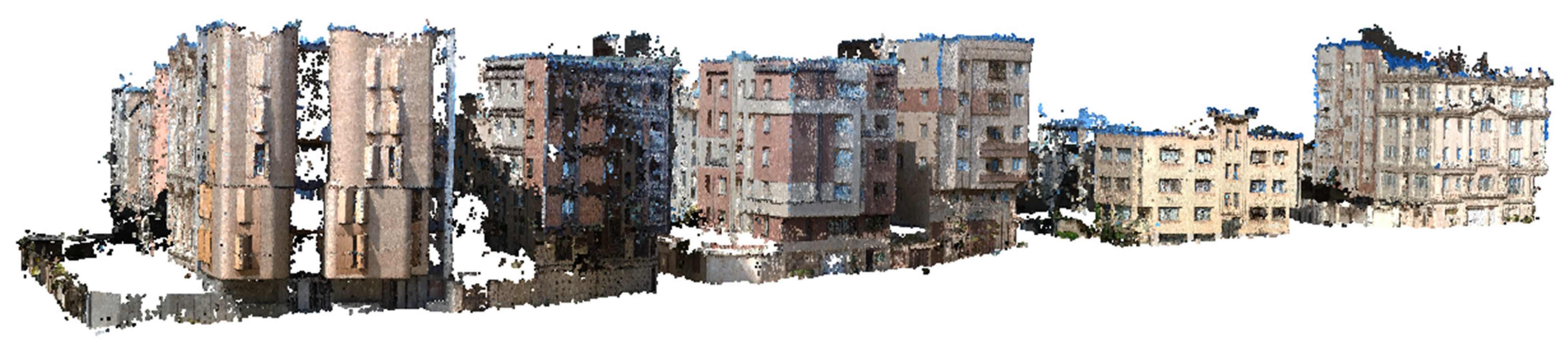
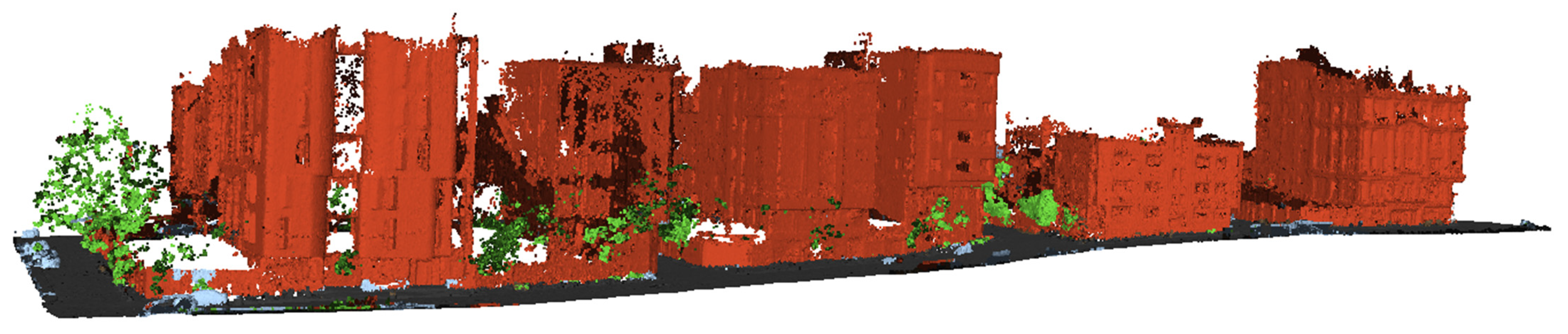
The production of point clouds in Metashape software is based on SFM-MVS techniques. Initially, a sparse point cloud is generated, followed by a dense point cloud. To create the sparse point cloud (3D reconstruction), key points are extracted and then matched to perform 3D reconstruction. Figure 5 displays the generated dense point cloud from four building blocks. Figure 6 illustrates the point cloud classified by the software, while Figure 7 depicts the class of the building.

Also,

Table 3. Numerical result of point cloud generated from four building blocks in the Agisoft Metashape software.

Output Results	Values
Accuracy of control scalebars	0.027 m
Accuracy of check scalebar	0.224 m
Reprojection error	1.28 pixels
The variance of the point cloud	0.24–0.56 m2

shows all the quantitative results of point cloud produced in Agisoft Metashape 2.0.2.

After generating the point cloud in the Meta shape software and saving the building class as output in LAZ format, the Cloud Compare software v2.12.0 is used to remove the noise of the point cloud. In order to make the point cloud calculations easier, it was moved from the UTM coordinate system to the local coordinate system defined by the software by applying shift (−1300, −3,953,000, −534,000).

Due to the large volume of the point cloud, to facilitate further processing, the point cloud is sampled at a distance of 10 cm, and finally the point cloud corresponding to 4 building blocks is exported separately in the PCD format and the local coordinate system.

2.3. Density-Based Analysis

In the 3D point cloud, density can be defined as the number of points per unit volume, and in the 2D point cloud, it can be defined as the number of points per unit area.

Considering that if the 3D point cloud of a building block is mapped in the X–Z plane, the intersection of vertical walls has a higher density than the surface of the wall, and also if the point cloud of the building block is mapped in the Y–Z plane, the intersection of horizontal walls has a higher density than the surface of the wall. This concept can be used to identify and extract the walls using the density analysis algorithm.

2.3.1. Orientation of the Main Walls

The prerequisite for extracting horizontal and vertical walls using density analysis is to first determine the directional angle of the point cloud using the Hough transformation and then rotate the point cloud along the z-axis using the rotation matrix so that the walls are parallel to the coordinate system axes. The basis of density analysis is the use of the simple geometric concept that walls are perpendicular to each other.

The point cloud is prepared in three steps as follows:

Step 1: Depth image generation and binarization

To identify the directional angle on a point cloud using the Hough transform, it is necessary to convert the point cloud into a binary image. First, the 3D point cloud is mapped in the x–y plane and a depth image is generated. To achieve this, the first 4 parameters must be specified as the resolution, minimum and maximum coordinates of the points, and the length based on Equation (1) and width based on Equation (2) of the generated image. Then, the average height of the points in a pixel is taken as its grey level (Figure 8a).

$$\mathrm{l}\mathrm{e}\mathrm{n}\mathrm{g}\mathrm{t}\mathrm{h}=\left({\displaystyle \frac{\mathrm{Y} \mathrm{m}\mathrm{a}\mathrm{x}-\mathrm{Y} \mathrm{m}\mathrm{i}\mathrm{n}}{\mathrm{R}\mathrm{e}\mathrm{s}\mathrm{o}\mathrm{l}\mathrm{u}\mathrm{t}\mathrm{i}\mathrm{o}\mathrm{n}}}\right)+1$$

(1)

$$\mathrm{W}\mathrm{i}\mathrm{d}\mathrm{t}\mathrm{h}=\left({\displaystyle \frac{\mathrm{X} \mathrm{m}\mathrm{a}\mathrm{x}-\mathrm{X} \mathrm{m}\mathrm{i}\mathrm{n}}{\mathrm{R}\mathrm{e}\mathrm{s}\mathrm{o}\mathrm{l}\mathrm{u}\mathrm{t}\mathrm{i}\mathrm{o}\mathrm{n}}}\right)+1$$

(2)

The next step is to convert the depth image into a binary image. All pixels that have a grey value are assigned a value of one and the other pixels are assigned a value of zero (Figure 8b).

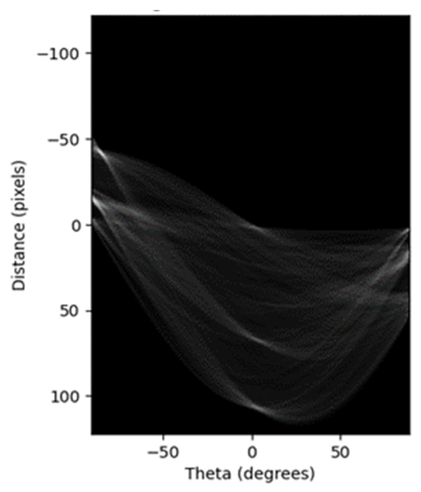
Step 2: Line detection using Hough transformation

The Hough transformation is used to identify simple shapes that can be specified with several parameters, such as lines, circles and ellipses.

In order to identify the direction angle one of the building blocks, it is necessary to implement the Hough transformation on the binary image of the building block (Figure 9).

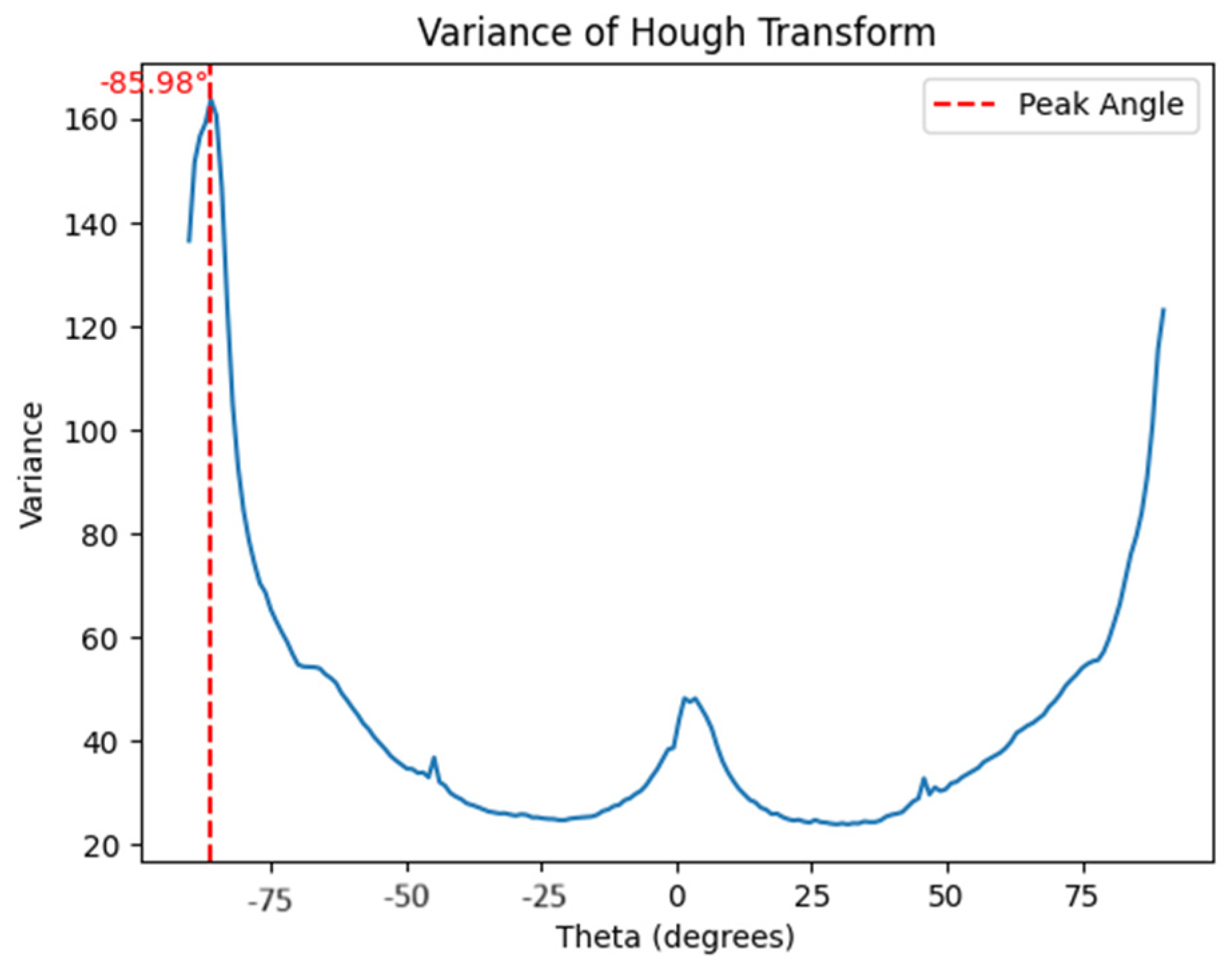
One of the limitations of line detection using the Hough transformation occurs when the number of lines is large, causing correlation errors around the peaks of the Hough space curves (Figure 9). As a result, increasing the number of lines leads to ambiguity in line identification. In order to find lines more easily, instead of detecting global maxima, local maxima are detected by plotting the variance graph of the columns of the accumulator matrix (Figure 10) and the largest local maximum in that dominant direction will represent the point cloud [26].

The obtained angle is the angle between the horizontal and vertical directions of the block. The difference between this angle and 90 degrees is the angle at which the walls of the block are placed parallel to the coordinate axes with the rotation of the point cloud.

Step 3: Rotation to the main orientation angle

After calculating the directional angle of the point cloud using the Hough transformation, which is equal to the peak (local maximum) of the variance graph of the columns of the accumulator matrix, the point cloud is rotated around the z-axis by the difference of this angle from 90 degrees using the rotation matrix (Equation (3)). As a result, the walls are placed parallel to the axes (Figure 11b) of the coordinate system and the first assumption for the use of the density analysis algorithm is established.

$$Rz(\theta )=\left( \begin{array}{ccc}cos\theta & -sin\theta & 0\\ sin\theta & cos\theta & 0\\ 0& 0& 1\end{array}\right)$$

(3)

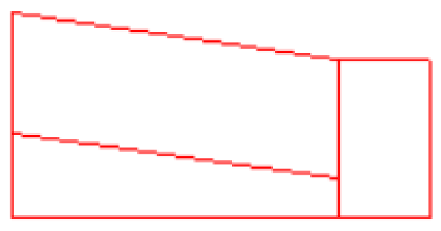
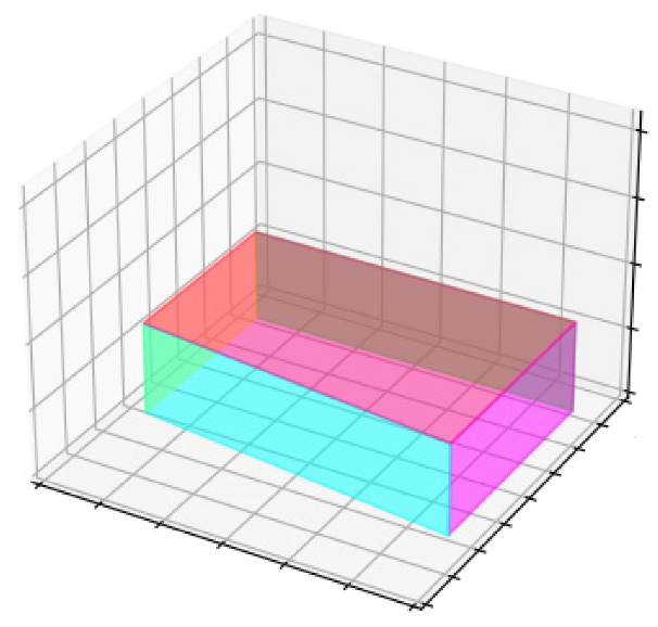
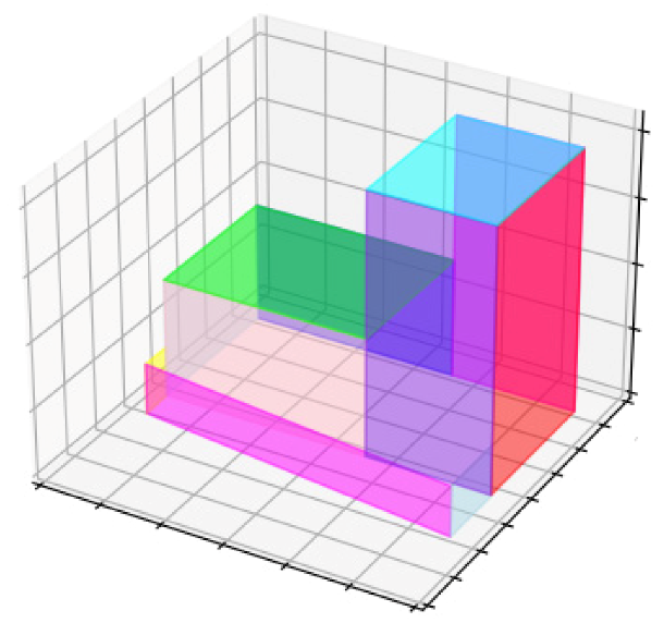
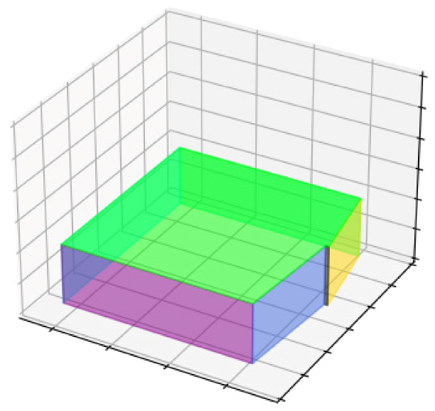
2.3.2. Extraction of Vertical Walls

In order to extract the lines of the vertical walls, it is necessary to go through three steps in the following order

• Point cloud mapping

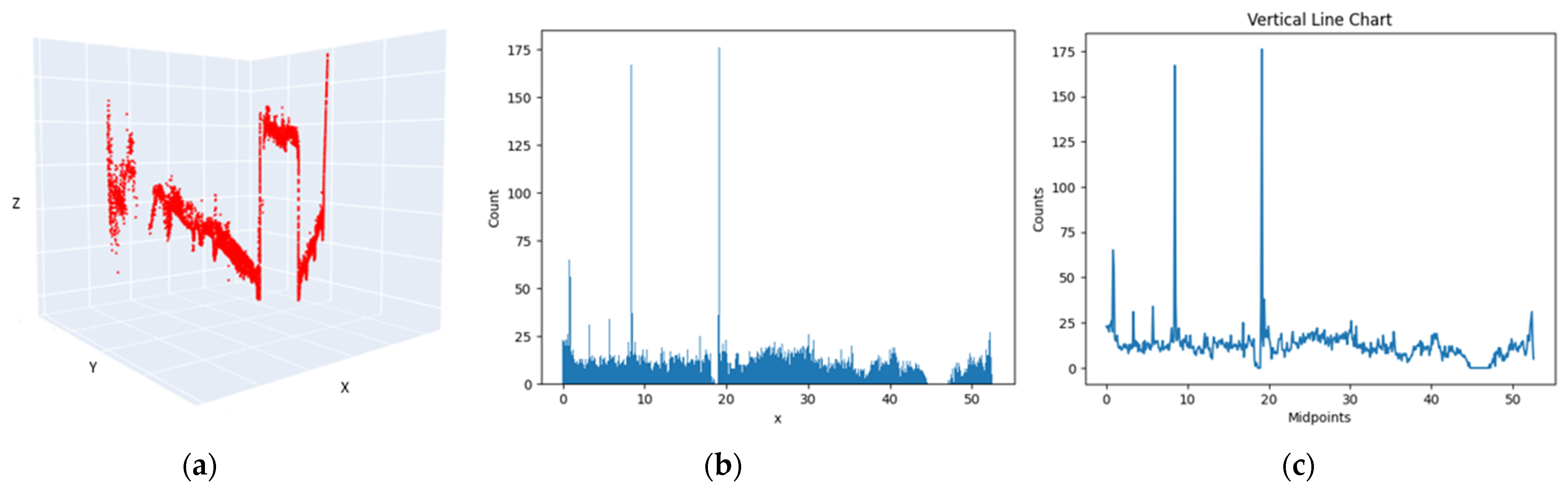
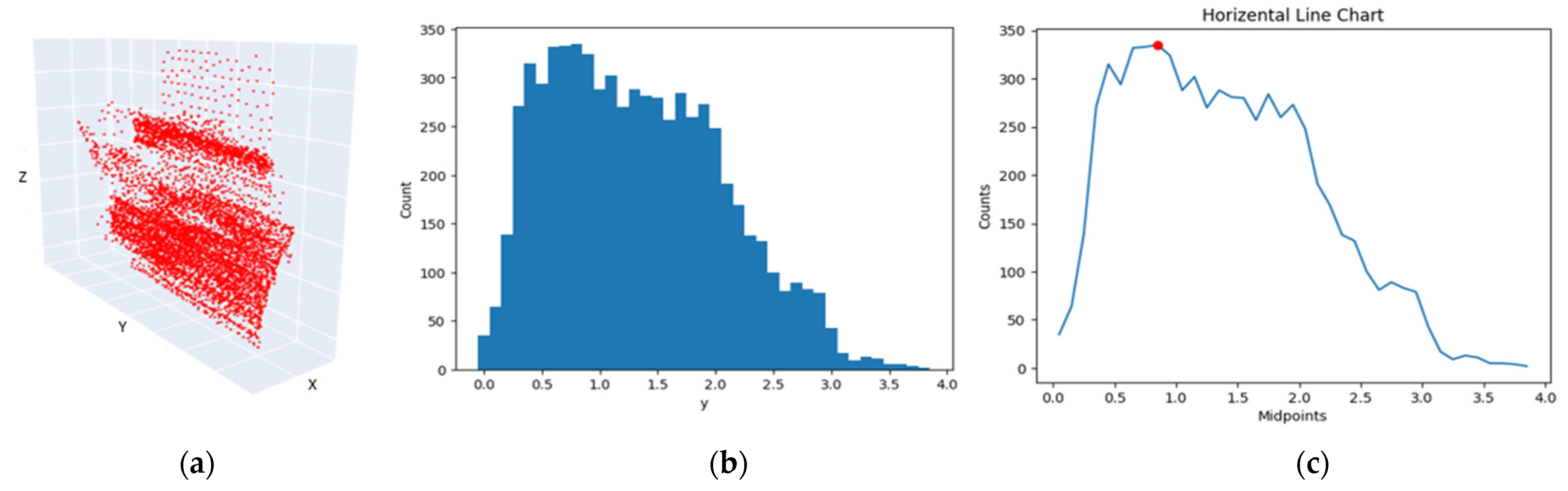
In the existing 3D point cloud, the y-value of all points is assumed to be zero (Figure 12a), so that the viewing angle to the point cloud is placed in the direction of the x-axis. In this direction, the intersection of the vertical walls will be displayed with greater density compared to the surface of the wall.

• Point cloud voxelization

The point cloud is voxelized along the x-axis by specifying the size of the voxels as one meter, and the histogram of the number of points in each voxel is drawn (Figure 12b). According to the national building regulations, the thickness of the main walls in brick and stone structures is 40 cm, but the point cloud of the building facade, doors and windows, and also the noise have caused the width of the main walls to be more than 40 cm. As a result, a voxel size of one meter was chosen as the optimal value, which produced corrected results in all 4-four data-sets.

• Drawing the density graph and identifying the peaks of the density graph:

The density graph is plotted along the x-axis according to the histogram created in the point cloud voxelization step. The peaks of the density graph are then determined, the peaks representing the highest density value in each voxel, and the highest density in the direction of the x-axis is given by the vertical walls (Figure 12c).

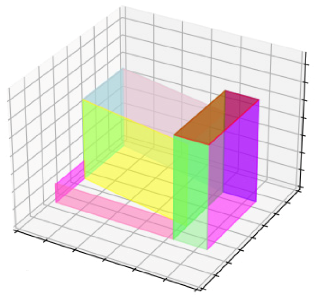
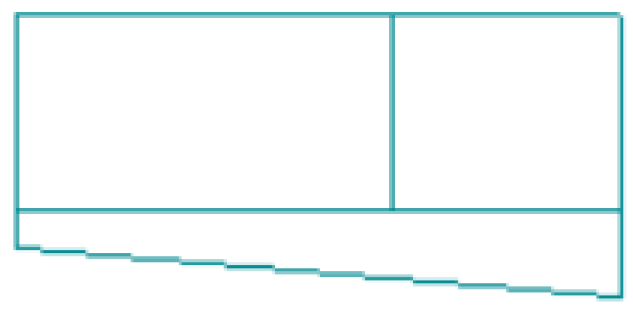
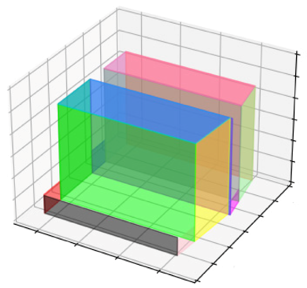
2.3.3. Extraction of Horizontal Walls

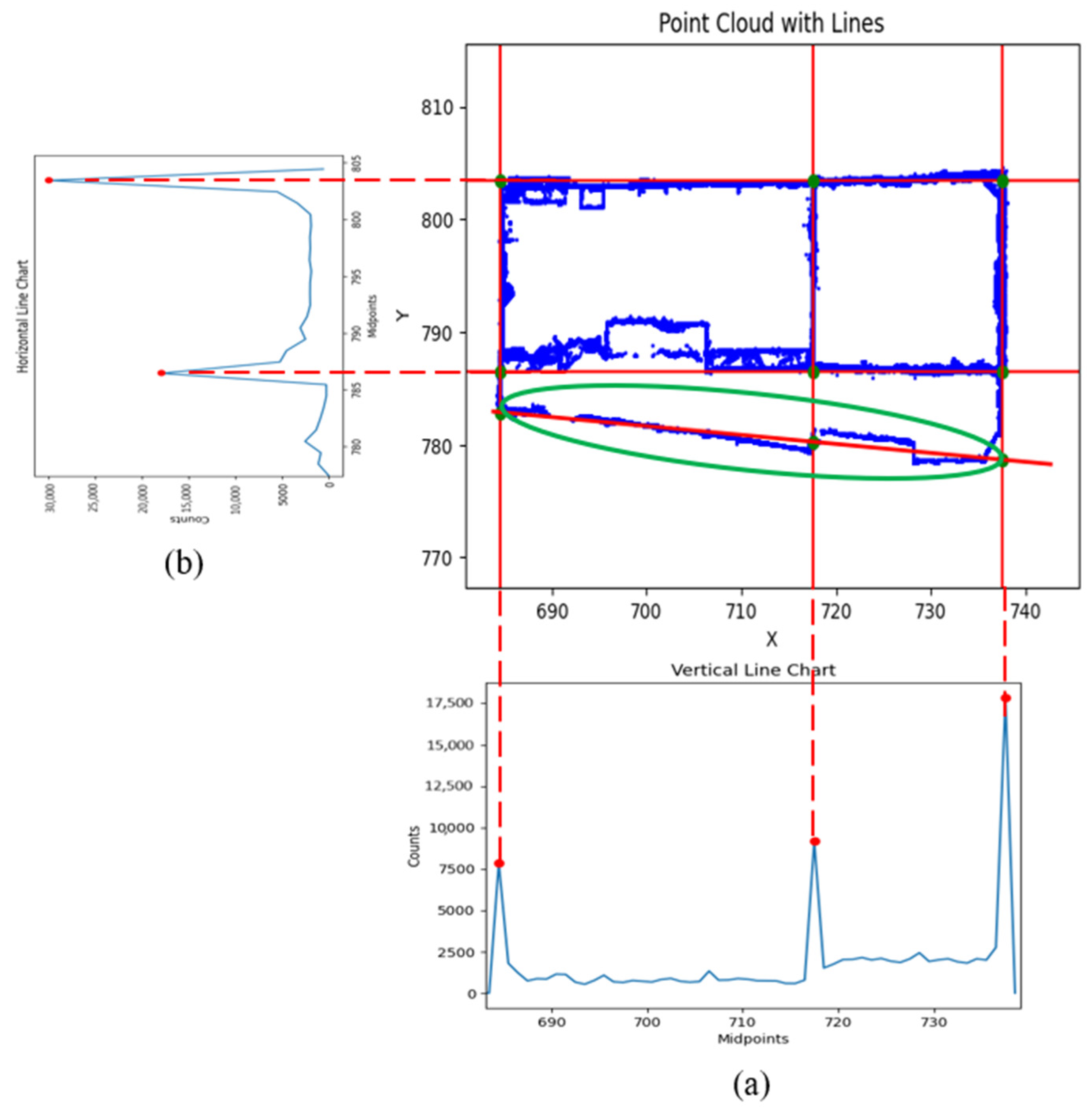
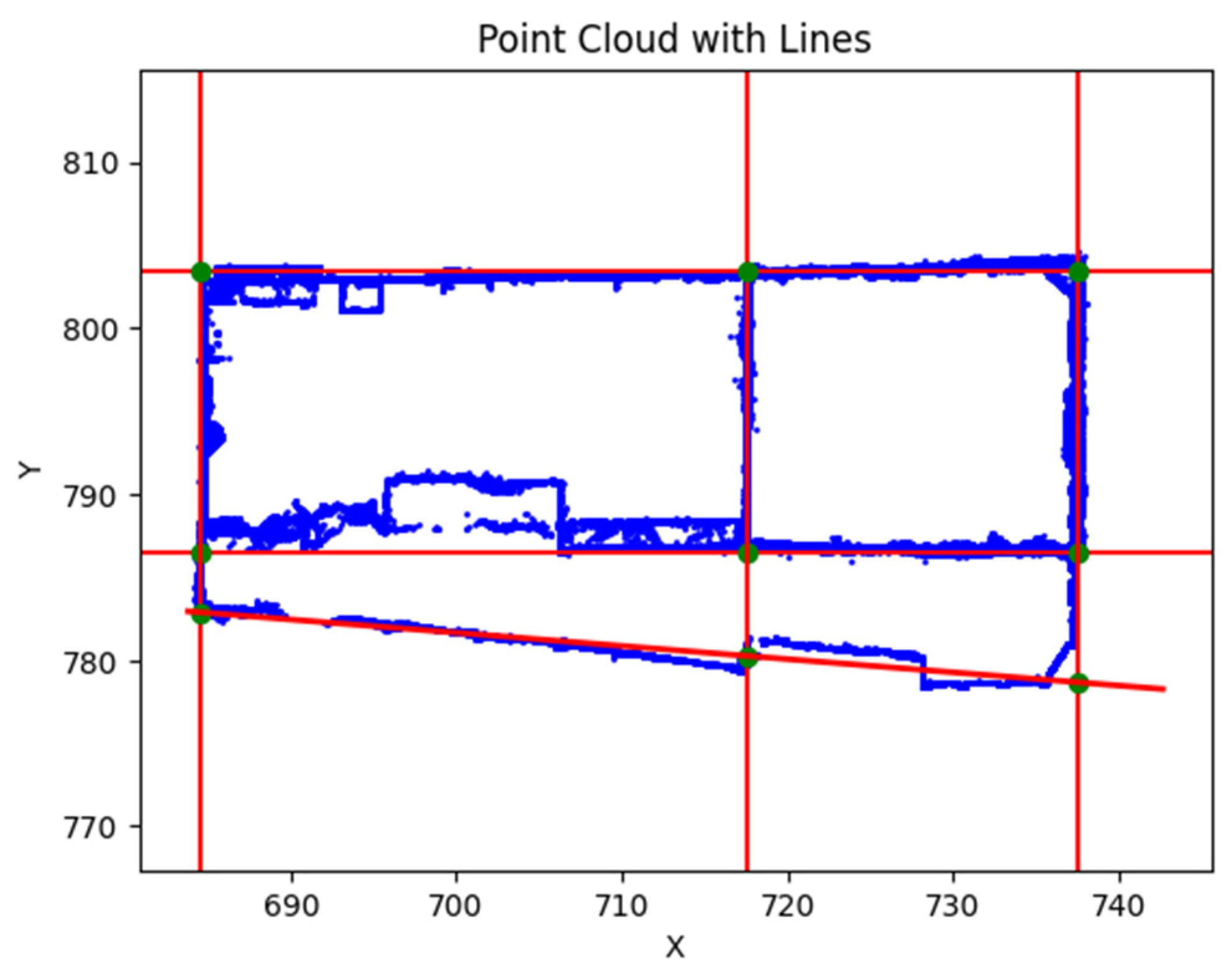
In order to extract the lines of existing horizontal walls in the point cloud of building block, the x-value of all points is assumed to be zero, so that the viewing angle to the point cloud is placed in the direction of the y-axis. In this direction, the intersection of the horizontal walls will be displayed with greater density compared to the surface of the wall. All the steps for extracting the lines of the horizontal walls, as shown in Figure 13, are the same as for the vertical walls in Section 2.3.2, except that the angle of view relative to the point cloud is adjusted in the direction of the y-axis. As a result, in (Figure 13c), the peaks represent the voxels with the highest density in the direction of the y-axis, and the highest density in the direction of the y-axis indicates the horizontal wall.

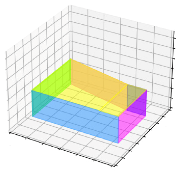
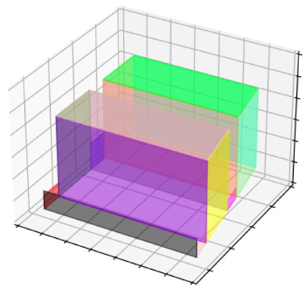
2.3.4. Extraction of Diagonal Walls

The lines of the diagonal walls are not directly obtained from the density analysis.

To extract the lines of the diagonal walls using density analysis, it is necessary to first use principal component analysis. Principal component analysis is a method of reducing data dimensions with minimal loss of accuracy. By retaining most of the changes in the primary data, this method transfers them to a new coordinate system so that the largest variance inthe data is placed on the first principal component (first axis) and the second largest variance is placed on the second principal component (second axis).

From a geometrical point of view, by applying principal component analysis to the point cloud related to the diagonal wall, the highest density of the point cloud is located in the direction of the first coordinate axis and the second highest density is located in the direction of the second coordinate axis.

In fact, the principal component analysis is performed on the diagonal wall to prepare the diagonal wall for the detection of the wall line using the density analysis method. As mentioned in Section 2.3.2 and Section 2.3.3, the vertical and horizontal wall lines were obtained by detecting the maximum density of the building block point cloud in the X and Y directions respectively.

As a result, since the diagonal wall is not in the direction of the main axes of the coordinate system (X and Y directions), the extension of the highest density associated with it is determined using the principal components analysis, i.e., the point cloud is placed in a new coordinate system so that the highest density is in the direction of the main axis in the new coordinate system.

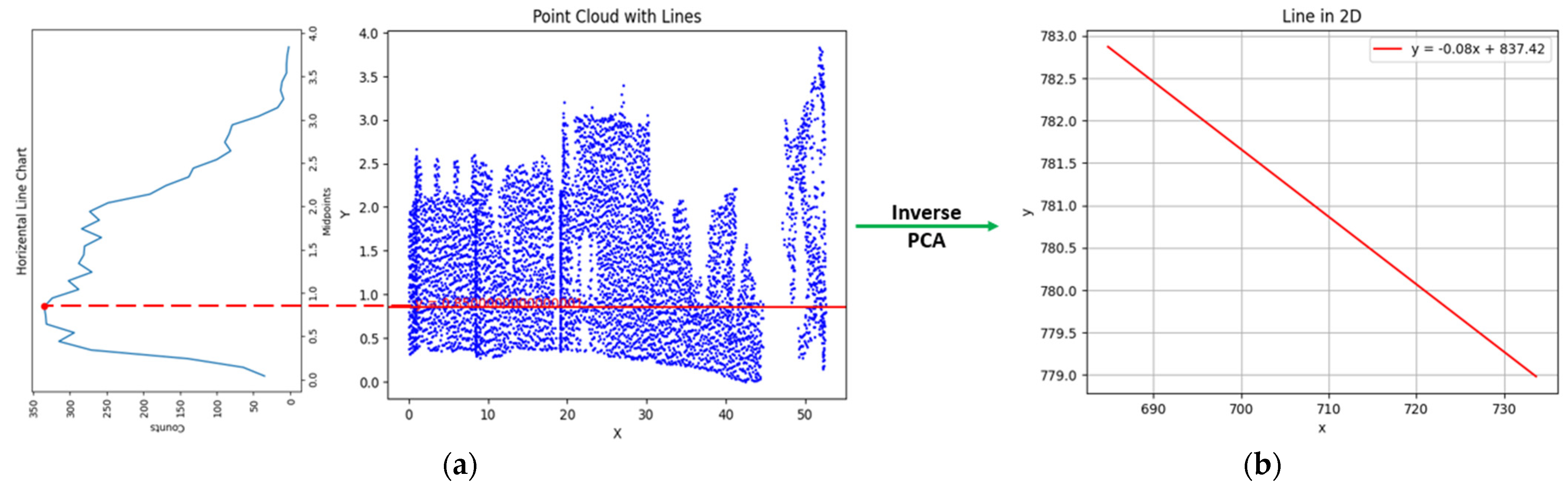
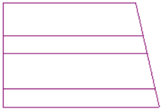
After transferring the point cloud of the diagonal wall to the new coordinate system using the principal component analysis, in the next step, the density analysis is implemented on diagonal wall as in Section 2.3.2, once in the direction of the x-axis (Figure 14) and again in the direction of the y-axis (Figure 15).

The density analysis performed on a diagonal wall in the new coordinate system in one direction is sufficient; the results show that when the diagonal wall extends along the horizon, according to the density graph (Figure 15c), the number of point (point cloud density) will be more in this direction. As a result, the peak shown in diagonal wall density graph in the new coordinate system in the Y direction (Figure 15c) represents the diagonal wall line.

3. Results

The results are explained in two sections, as follows: in Section 3.1, the results of density analysis are explained, and in Section 3.2, the evaluation results are explained.

In Section 3.1, the final output of the point cloud density analysis of the building block is discussed during the process of extracting the lines of the horizontal, vertical and diagonal walls, and at the end, the 2D plan in shapefile format, the prismatic model and the 3D model produced for four building blocks are displayed. In Section 3.2, the accuracy of the produced model of four building blocks is checked using density analysis of the ratio of real sizes, and a visual comparison of the 2D plan produced using density analysis with the open-source map of Tehran municipality is presented.

3.1. Result of Density-Based Analysis

In the first step, by designing a network with ground stations at a distance of two meters and crossing the center line of the street, images of four building blocks were taken using the Insta 360 One X2 spherical camera.

As mentioned in Section 2.1, in the first step of designing a network with ground stations at a distance of two meters from each other and crossing the center line of the street, the images of four building blocks were taken using the Insta 360 One X2 spherical camera. In the second step (Section 2.2), the Metashape software was used to generate a point cloud of the building class (Figure 7) from an equirectangular image.

In the third step (Section 2.3), a density analysis was conducted on the point cloud of a building block with the objective of extracting the lines of the external walls. In order to utilize the density analysis algorithm for the extraction of external wall lines, it is essential that the point cloud is justified in a manner that ensures the walls are parallel to the coordinate axes (Section 2.3.1). In order to extract the lines of the vertical walls of the point cloud (Section 2.3.2), it was mapped on the X-Z plane and vowelized along the X-axis at one-meter intervals. Subsequently, a density graph was constructed based on the aforementioned voxelization. This graph illustrates the number of points within each voxel. The peaks of the density graph correspond to the lines of the vertical walls of the building block (Figure 16a). This is because upon mapping the point cloud in the X-Z plane, the intersection of the vertical walls is displayed with a higher density than the surface of the wall. In order to extract the lines of the horizontal walls (Section 2.3.3), all the steps previously implemented in the extraction of the lines of the vertical walls are repeated in the direction of the y-axis (Figure 16b).

The issue that requires further investigation is that the density analysis was only able to extract the lines of the horizontal and vertical walls, and the diagonal wall lines highlighted in green in Figure 16 were not extracted. As outlined in Section 2.3.4, diagonal wall lines cannot be obtained directly through density analysis. Consequently, initially it is necessary to separate the point cloud corresponding to the diagonal walls from the main point cloud. To do this, according to the coordinates of the points obtained from the intersection of the equation of the line corresponding to the lines of the horizontal and vertical walls in Figure 16, by specifying a y interval for horizontal lines and an x interval for vertical lines, the horizontal and vertical walls are removed from the main point cloud, leaving only the point cloud of the diagonal wall.

The point cloud of the diagonal wall is transferred to a new coordinate system using principal component analysis. The geometric nature of this transformation makes the maximum density of the point cloud to be aligned with the first principal component. Density analysis in this direction then allows the equation of the diagonal wall line in the system to be calculated (Figure 17a). Ultimately, the objective is to obtain the diagonal wall line in the original coordinate system. This is achieved through the application of the inverse principal component analysis (Figure 17b).

At last, the 2D plan of the building block is created by intersecting the lines of the vertical, horizontal and diagonal walls, which have been obtained through the analysis of the point cloud density.

In accordance with the equations and the intersection of the wall lines in Figure 18, the 2D plan of the building block can be produced in the shapefile format. Furthermore, by considering the lines of the outer walls and applying the average height of the point cloud on the wall lines, a prismatic model can be produced. Additionally, despite the point cloud of the building block having been classified in Agisoft Metashape and denoised in Cloud Compare software 2.0.2, residual point clouds of the sky and ground remain. Specifically, these are present in the upper and lower parts of the walls.

Subsequently, the value of the component was sorted in descending order of the point cloud, with the top and bottom 2% removed to denoise the point cloud. Thereafter, the intersection of the walls was identified through the phase of detecting wall lines using density analysis. Based on these coordinates, the height of each wall was obtained from the existing point cloud and applied to the 2D plan to obtain the 3D model.

Table 4. The 2D plan, 3D models and prismatic model of four building blocks.

Number of Block	Prismatic Model	3D Model	2D Plane
Block1
Block2
Block3
Block4

presents the 2D plan, prismatic model and 3D model of four building blocks.

3.2. Validation

In order to assess the accuracy of the model of the four building blocks produced in relation to real size, a number of widths and heights of the accessible walls, the majority of which belong to the courtyard walls of the northern houses, were measured using a laser meter.

Table 5. Horizontal, vertical and total precision compared to the actual values measured with a laser meter.

Length Accuracy (m)	Height Accuracy (m)	Total Accuracy (m)
0.325	0.090	0.442

shows the length, height and total accuracy of the 3D model created using the presented algorithm, compared to the actual values measured with a laser meter, and a detailed examination of these values is provided below.

According to Section 2.2, the point cloud has been transferred from the UTM coordinate system to the local coordinate system; as a result, the 2D plan produced also has local coordinates and by applying the shift (1300, 3,953,000, 534,000), the 2D plan is returned to the UTM coordinate system.

The 2D plan is also rotated as described in Section 2.3.1. At this stage, it is rotated by the inverse of the angle to return to its original position. The resulting map is saved in shape file format.

The open-source map of Tehran municipality https://map.tehran.ir (accessed on 5 September 2023) is available in jpeg format in Arc GIS software 10.8. It has been georeferenced using three points in the UTM coordinate system. The shape file of the building blocks has then been overlaid on the existing map. A visual comparison of the 2D map produced with the existing map can be seen in Figure 19.

A visual comparison of the generated map with the municipality map in Figure 19 reveals that the greatest difference in length is associated with the corner of the building block, which in reality is round. In fact, the proposed algorithm could not extract the corners of the buildings in a rounded form, and according to Table 5, this problem has led to a slight error in the horizontal accuracy. However, the height accuracy, obtained by comparing the height of the accessible walls of the northern houses with the generated 3D model, is a desirable accuracy. Thus, it can be concluded that the presented algorithm has provided good accuracy in the extraction of vertical walls.

A comparison was conducted between the length of the external walls in the 2D plan and the corresponding walls in the map, using the measurement tool available on the Tehran municipality website. The precision of the 2D plan produced was estimated to be 0.311 m.

The wall between the buildings in each block was drawn from the map of Tehran municipality in ArcMap software10.8 (Figure 20a). A width of 40 cm was applied to the walls and the lines of the walls were extruded according to the average height of the three-story buildings above and below the three-storybuildings in the existing point cloud. The final model, Figure 20b, was produced in SketchUp2021 software.

4. Discussion and Conclusions

While the 3D modeling of urban building blocks is often generated using aerial and satellite imagery to cover large-scale urban areas, the vertical and oblique viewing angles of these data sets result in buildings with complex roofs. This presents a challenge for the accurate identification of building wall lines in applications such as cadastre, while the cost of flying and increasing the resolution of satellite imagery is a significant barrier.

Therefore, the Insta 360 One X2 spherical camera is utilized, which is one of the more cost-effective sensors, with a field of view of 360 × 180° degrees and the ability to capture the entirety of the surrounding environment in a single image, by using a limited number of images of four building blocks. To cover a city, and as a result of modeling with a lower number of images, computation time and data volume, the accuracy (reprojection error) of point cloud reconstruction in Agisoft Metashape software is reported to be 3.210 pixel in a single-story cultural heritage building [8]. The reconstruction of four building blocks in Agisoft Metashape software (Table 3) in an area of 740 square meters yielded an accuracy of 1.28 pixel. This is due to the fact that the images used to generate the point cloud from the Insta 360 One X2 camera were pre-calibrated using commercial camera software (Insta 360 studio 2023), whereas the Ricoh Theta camera in study [8] was not calibrated, even though the control points were used.

It is important to acknowledge that more advanced methods, such as LiDAR or high-resolution drone photogrammetry, are capable of achieving sub-centimeter accuracy. However, these methods come with significantly higher costs and longer processing times.

A quantitative comparison with state-of-the-art techniques reveals a clear trade-off between cost, time efficiency and accuracy. To illustrate, LiDAR is capable of generating highly dense point clouds with remarkable precision; however, the associated equipment and data processing are both costly and time-consuming. Similarly, drone-based photogrammetry can achieve high accuracy, especially when paired with ground control points (GCPs). However, it still demands considerable effort in terms of image acquisition, large data volumes and intensive post-processing. In comparison, the Insta 360 One X2 camera represents a compromise between cost and efficiency. It necessitates fewer images to cover urban areas, offers accelerated processing times, but exhibits a degree of compromise in terms of accuracy. In instances where the highest accuracy is of paramount importance, more sophisticated methods may be required. However, for cost-effective urban management tasks, the spherical camera approach remains a viable and efficient alternative.

The presented algorithm for generating a 3D model is one of the data-driven modeling techniques, which is based on the density of the point cloud generated from spherical camera images, is a method that demonstrated that, under the assumption that changing the viewing angle in both horizontal and vertical directions lead to the intersection of the walls with a higher density than the surface of the wall. If the point cloud is displayed in a reduced density, it can still be identified by changing the viewing angle relative to the exterior walls from the facade of the building. One of the limitations of the presented method is the difficulty in extracting the lines of diagonal walls. This is because diagonal walls often have less point cloud density along the main coordinate axes (X and Y), making it harder to find them. To address this challenge, the current article proposes using Principal Component Analysis (PCA) to find the highest point cloud density along the primary axis of the new coordinate system. However, further improvements can be advanced machine learning algorithms for automated feature extraction could be employed to better detect and delineate diagonal structures. Combining PCA with these techniques may offer a more robust solution to the limitations of the current method, leading to more accurate 3D models.

After extracting the lines of the external walls and the intersection of these lines with each other, the 2D plane of the building block was produced, and according to the intersection of the lines, the height of each of the walls was obtained from the point cloud and the walls were extruded to produce a 3D model, the horizontal and vertical accuracy of the produced 3D model compared to reality were 32 and 9 cm, respectively.

Future research could focus on developing a robust calibration method tailored specifically for both equirectangular and fisheye images. The aim would be to enhance the accuracy and reliability of 3D models generated from spherical camera images that do not conform to traditional perspective geometry. Such a calibration method would assist in the mitigation of the distortions inherent to spherical imaging, thereby enhancing the overall precision of point cloud-based reconstructions.

Furthermore, a significant proportion of the algorithms utilized during the modelling process, including those employed for key point extraction, are primarily designed for images with perspective geometry. Further research could investigate the adaptation or development of new algorithms for diverse panoramic image geometries, such as equirectangular images. By refining both classical and deep learning algorithms for these non-perspective geometries, researchers could significantly enhance the efficacy of 3D reconstruction techniques for spherical and panoramic imaging systems.

Another area meriting future investigation is that of the indistinguishability of lines between buildings within the same block, which arises from the ground-based nature of data acquisition and the generation of building façades as point clouds. Further research could examine methods of enhancing the distinction of these boundary lines, potentially through the integration of aerial drone data with ground-level imaging. The combination of drone-acquired data with ground control points (GCPs) could enhance the geometric strength and accuracy of the models, facilitating more detailed and accurate representations of complex urban environments.

Also, given the importance of 3D reconstruction of urban buildings in the field of urban management, texture mapping from spherical camera images is one of the tasks that can be addressed in the future.