Abstract
Zenith Tropospheric Delay (ZTD) is a significant error source affecting the accuracy of certain space geodetic measurements. This study evaluates the performance of Artificial Intelligence (AI) based meteorological models, such as Fengwu and Pangu, in estimating real-time ZTD. The results from these AI models were compared with those obtained from the Global Navigation Satellite System (GNSS), the fifth-generation European Centre for Medium-Range Weather Forecasts (ECMWF) Atmospheric Reanalysis (ERA5), and the third generation of the Global Pressure–Temperature data model (GPT3) to assess their accuracy across different time intervals, seasons, and geographic locations. The findings reveal that AI-driven models, particularly Fengwu, offer higher long-term forecasting accuracy. An analysis of data from 81 stations throughout 2023 indicates that Fengwu’s 7-day ZTD forecast achieved an RMSE of 2.85 cm when compared to GNSS-derived ZTD. However, in oceanic regions and areas with complex climatic dynamics, the Fengwu model exhibited a larger error compared to in other land regions. Additionally, seasonal variations and station altitude were found to influence the accuracy of ZTD predictions, emphasizing the need for detailed modeling in complex climatic zones.
1. Introduction
Tropospheric delay is a significant error in space geodetic techniques such as those performed by the GNSS, Very-Long-Baseline Interferometry (VLBI), Satellite Laser Ranging (SLR), and Interferometric Synthetic Aperture Radar (InSAR) [1,2,3,4,5]. Therefore, understanding the properties of the troposphere is essential for enhancing the accuracy of these geodetic techniques. The troposphere is the lowest layer of the atmosphere, extending up to approximately 50 km [6]. This layer contains the majority of the atmosphere’s water vapor and aerosols, which refract electromagnetic wave signals, leading to elongated signal paths and reduced propagation speeds. Tropospheric delay is typically quantified as ZTD and projected onto the line-of-sight direction of observations using specific projection functions. The accurate assessment and correction of tropospheric delay are critical not only for improving the precision of space geodetic measurements but also for enhancing the overall reliability of atmospheric models and climate studies.
Current methodologies for obtaining ZTD encompass a range of techniques, including external observations, empirical models, meteorological empirical models, reanalysis data, and numerical weather predictions. Instruments like radiosondes and water vapor radiometers are traditionally used to observe tropospheric delay, but these methods can be costly and may lack the desired spatial and temporal resolution [7,8]. Alternatively, satellite observations can provide high-resolution data [9]; however, their accuracy may be compromised under extreme weather conditions, where precise tropospheric delay information is particularly critical [10].
Empirical models, which do not depend on external data, use specific input parameters to estimate ZTD values [11,12,13,14,15,16,17,18,19,20,21]. These models are widely utilized due to their convenience, with the GPT series of models being notably influential, now in its third generation [22,23,24,25]. Nevertheless, these models face limitations in accuracy, especially concerning real-time meteorological conditions. Meteorological empirical models, like those developed by Hopfield, Saastamoinen, and Black, require external meteorological data inputs to calculate tropospheric delay [26,27,28]. Reanalysis data, such as the ERA5 data, offer relatively high accuracy for ZTD calculations but are limited by a five-day data lag [29]. Numerical forecast products, exemplified by the Global Forecast System (GFS) from the National Centers for Environmental Prediction (NCEP) in the United States, provide another method for estimating tropospheric delay, albeit with significant computational demands and generally lower accuracy compared to ERA5 [30,31].
Recent advancements in AI have opened new avenues for numerical weather forecasting. AI-based meteorological models have demonstrated substantial improvements in the accuracy and efficiency of meteorological forecasts [32,33,34,35,36,37]. At the same time, it is recognized that AI meteorological models are still in the initial stage [38,39]. AI-based weather prediction models, such as Google’s GraphCast [34], NVIDIA’s FourCastNet [40], Huawei’s Pangu [41], the Shanghai Artificial Intelligence Laboratory’s Fengwu model [32], and Fudan University’s Fuxi model [35], have demonstrated significant improvements in forecasting accuracy and efficiency. These models leverage AI algorithms to enhance prediction precision and accelerate inference processes. The outputs of these models consist of gridded discrete meteorological parameters, and further evaluation of their performance is necessary to integrate them into geodetic applications. Wuhan University’s TropNet model also employs deep learning techniques, utilizing data from the Geostationary Operational Environmental Satellite-R (GOES-R) series and NCEP’s GFS to predict zenith wet delay (ZWD), marking a promising initial application of AI algorithms in the tropospheric domain [37]. Comparative analyses by researchers such as Xu et al. indicate that the Pangu model outperforms the GFS in predictive performance [42]. Chen et al. found that the Fengwu model surpasses GraphCast in predicting 80% of the 880 reported predictands [32]. Additionally, Charlton-Perez et al. conducted a performance analysis of Pangu, GraphCast, FourCastNet, and FourCastNet V2 [39]. While these studies focus primarily on weather forecasting capabilities, there remains a gap in assessing the applicability of AI weather models in addressing tropospheric errors within geodetic methods, warranting further investigation.
This study selects the Pangu and Fengwu models as representatives and employs a hybrid integration algorithm to explore their potential in calculating tropospheric delays. We evaluate the accuracy of the models’ inversion results using data from GNSS stations, aiming to demonstrate the efficacy and reliability of AI-driven approaches in this domain. While these AI meteorological models are still in their infancy, they represent a significant leap forward in the computation of tropospheric products, holding promise for further advancements in the accuracy and timeliness of space geodetic measurements.
2. Data and Model
The scope of this study is global, utilizing specific data sources including ERA5 pressure level data, GNSS station positions provided by the International GNSS Service (IGS), and ZTD data. The Fengwu and Pangu models were selected for the AI meteorological models due to their long forecast duration, high resolution, and superior accuracy. For comparison, the GPT-3 model was also included.
2.1. ERA5 Data
This study utilized the ERA5-Land hourly data from 1950 to the present and the ERA5 hourly data on pressure levels from 1940 to present, which are reanalysis datasets provided by the ECMWF through the Copernicus Climate Change Service (C3S), (https://cds.climate.copernicus.eu/datasets?q=ERA5, accessed on 13 October 2024). These data can be used both to provide the initial background fields for AI weather models and to calculate ZTD for data comparison. In this study, we primarily focused on global data from the year 2023, covering the temporal range from 1 January to 31 December. The data have a spatial resolution of 0.25° × 0.25° and provide global coverage, spanning latitudes from 90°N to 90°S and longitudes from 0°E to 360°E. The variables used in this analysis include pressure, temperature, specific humidity, and geopotential height. The original ERA5 dataset includes 37 pressure levels, but, for consistency with the input data format requirements of the Fengwu and Pangu models, we extracted data for 13 selected pressure levels (1000, 925, 850, 700, 600, 500, 400, 300, 250, 200, 150, 100, and 50 hPa). The ERA5 data were primarily used as the initial background field for the Pangu and Fengwu models and also served as reference data for verifying the ZTD values calculated from these models.
2.2. GNSS ZTD Data
The GNSS data used in this study were sourced from the Wuhan University IGS Analysis Center (http://www.igs.gnsswhu.cn/index.php, accessed on 13 October 2024). The ZTD data from the IGS center are characterized by high accuracy and reliability [43]. During data verification, some station data were found to be incomplete. After excluding stations with incomplete data from 2023, a total of 81 stations with complete ZTD data for the entire year remained. Therefore, this study utilized ZTD data from these 81 global stations, sampled every 5 min. In this research, GNSS ZTD data serve primarily as a reference to validate the ZTD data generated by AI meteorology models.
2.3. Pangu-Weather Model
The Pangu-Weather model is an advanced AI-based meteorological model developed by Huawei (https://github.com/198808xc/Pangu-Weather, accessed on 13 October 2024). It employs a neural network architecture trained on a vast number of historical weather data and ERA5 reanalysis data. The model is capable of generating high-resolution weather forecasts by learning complex atmospheric patterns and relationships. Pangu’s outputs include standard meteorological variables such as temperature, specific humidity, wind speed, and pressure, among others. It has demonstrated a high level of accuracy in forecasting, often outperforming traditional numerical weather prediction models, particularly in short-to-medium-range forecasts. A key advantage of the Pangu model is its computational efficiency, allowing it to produce forecasts significantly faster than traditional models. Additionally, it can integrate diverse data sources, making it versatile for various meteorological applications. In this study, the accuracy of the ZTD calculations generated by the Pangu model was compared with that produced by the Fengwu model.
2.4. Fengwu-Weather Model
The Fengwu-Weather model, developed by the Shanghai Artificial Intelligence Laboratory, is an advanced AI-driven global weather forecasting model (https://github.com/OpenEarthLab/FengWu, accessed on 13 October 2024). Each data instance has a shape of 69 × 721 × 1440, representing 69 atmospheric features, 721 latitude points from 90°N to 90°S, and 1440 longitude points from 0° to 360°. The model includes surface variables (10 m V-Component of Wind, 10 m U-Component of Wind, 2 m temperature, and mean sea level pressure) followed by non-surface variables (geopotential, specific humidity, V-Component of Wind, U-Component of Wind, and temperature) at 13 vertical levels (50, 100, 150, 200, 250, 300, 400, 500, 600, 700, 850, 925, and 1000 hPa). In this study, the non-surface variables to compute ZTD using a hybrid integration algorithm are utilized, and the accuracy of the inversion results with GNSS station data is evaluated.
2.5. GPT3 Model
The GPT3 model is the third generation of the GPT series (https://vmf.geo.tuwien.ac.at/products.html, accessed on 13 October 2024). It is based on statistical and empirical methods, incorporating historical meteorological data and geographical information while also considering factors such as topography and seasonal variations. This model provides estimates of global temperature and pressure, as well as ZTD estimation. In this paper, the ZTD data from the GPT3 model with those from an AI meteorological model are compared.
3. Methodology
To generate real-time ZTD using an AI meteorological model, two main steps are required. First, the AI meteorological model is used to obtain predicted meteorological parameters. Then, the integration method, along with the predicted meteorological parameters, is utilized to calculate the ZTD at points of interest. Due to the 5-day delay in the ERA5 product, and the fact that AI meteorological models require ERA5 to provide the initial background field, the initial field time by retroactively subtracting 5 days from the target time is utilized. The Pangu model requires only one initial background field, while the Fengwu model needs two initial background fields, with a 6 h interval between them. Therefore, the additional initial background field for the Fengwu model should be 5 days earlier, plus an additional 6 h. The forecast results from the AI meteorological models are then used as the initial conditions for the subsequent forecast, continuing this process until the meteorological parameters for the observation day are obtained. The required ZTD values for the specified period can be calculated using numerical integration. If a finer temporal resolution of ZTD is needed, interpolation methods can be applied to refine the time information. The specific calculation approach is illustrated in Figure 1.
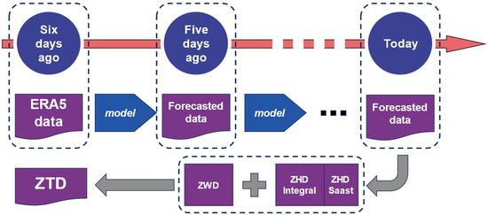
Figure 1.
Schematic diagram for obtaining ZTD using the AI meteorological model.
3.1. Integration Calculation of ZTD
Several scholars have studied the integration method for calculating, but there are differences in the details [44,45,46]. The is composed of two components: the Zenith Hydrostatic Delay () and [6].
where meteorological parameters, forecasted by the AI meteorological model, are utilized to perform integral calculations of and according to different pressure levels [46]. The formula for computing is as follows:
where is the height of the observation station over mean sea level (unit: meters). is the hydrostatic refractivity (unitless). The unit of the is meters. Similarly, (unit: meters) can also be obtained through integration:
where has the same meaning as above. is the wet refractivity (unitless). and can be modeled as follows [47]:
In the above formulas, , , and are the refractivity constants. , , and [47]. is the temperature (unit: kelvin). is the air density [48]:
where and are the gas constants for dry air and water vapor, respectively. In the above formulas, and are the dry air and water vapor partial pressures (unit: hPa), respectively. can be obtained by subtracting from the total atmospheric pressure (unit: hPa), where is acquired as follows [49]:
where is the specific humidity (unit: kg/kg). Finally, the segmented integration method is adopted to obtain the final and . Prior to integration, interpolation is performed on , , , and with a 10 m interval.
where denotes the height of a given layer (unit: meters). and are the hydrostatic and wet refractivity values at a given layer , respectively. The values of the and are within the specified altitude range. For the unmodeled above the specified range, estimation is carried out using the meteorological parameters at the top layer and the Saastamoinen model [27].
where is the top-layer atmospheric pressure, is the top-layer height, and is the latitude of the interest point. Therefore, the final can be obtained through the following method:
3.2. Calculation Strategy of the AI Meteorological Model
To run the AI meteorological model, an initial background field is required, encompassing both surface-layer and upper-atmosphere data. The surface-layer data are sourced from the ERA5-Land hourly data dataset, while the pressure level data are derived from the ERA5 hourly data on pressure levels dataset. For the surface layer, the key parameters include the 10 m U-Component of Wind (u10), 10 m V-Component of Wind (v10), 2 m temperature (t2m), and mean sea level pressure (msl). For the upper layers, the model utilizes data on geopotential (z), specific humidity (q), the U-Component of Wind (u), the V-Component of Wind (v), and temperature (t). The surface and upper datasets are merged to form a comprehensive dataset. The dataset dimensions are 69 × 721 × 1440, where 69 represents the 69 atmospheric features. The first four variables are surface variables, namely [‘u10’, ‘v10’, ‘t2m’, ‘msl’]. The remaining variables are upper variables, specifically [‘z’, ‘q’, ‘u’, ‘v’, ‘t’]. Each upper variable includes 13 different atmospheric levels, which are [50, 100, 150, 200, 250, 300, 400, 500, 600, 700, 850, 925, 1000] hPa. As mentioned earlier, the Fengwu and Pangu models require a different number of initial fields, but their data structures are the same. The Fengwu model as an example to explain the process of predicting data will be used. The Fengwu model can predict and output various meteorological parameters, as illustrated in Figure 2.
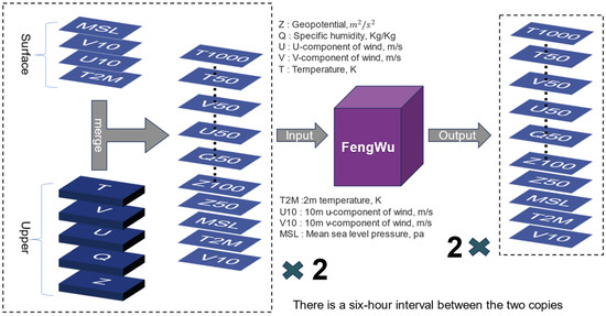
Figure 2.
Schematic diagram of the Fengwu meteorological model operation.
The output format of the Fengwu model is consistent with the input format, both being gridded data. The operational workflow of the Fengwu model requires two initial background fields with a 6 h interval between them. These initial fields can be obtained from ERA5 data. By running the Fengwu model, the forecast is made for 6 h after the most recent initial background field. For example, if the initial background fields are at 2:00 and 8:00, the model will generate forecast data for 14:00. Then, using the data from 8:00 and 14:00, the Fengwu model will generate data for 20:00. This process continues iteratively, rolling forward to obtain the forecast for the target time. The Fengwu model significantly enhances forecasting skills, extending the lead time for accurate medium-range global weather predictions to 10.75 days (with an ACC of z500 > 0.6) [32]. The calculation process schematic diagram is shown in Figure 3.
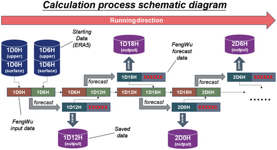
Figure 3.
The calculation process schematic diagram.
The Pangu model requires only one initial background field. The forecast model is selected based on the target time, and the initial background field is used to predict the results. This result is then input into the specified model, and the process continues until the forecast for the target time is obtained. It is important to note that Pangu provides models with 1 h, 3 h, 6 h, and 24 h time steps. The combination principle is to minimize the number of model calls. For example, if the forecast is for 5 days and 4 h later, the optimal combination would involve five 24 h models, one 3 h model, and one 1 h model. This approach minimizes the number of model calls and also helps avoid error accumulation [41].
After obtaining the meteorological parameters, since both the Fengwu and Pangu models provide gridded data, further steps are required to retrieve the ZTD for a specific point of interest. First, the grid cell containing the point of interest is identified, and the heights of the grid corners are adjusted to match that of the point of interest. Then, using the numerical integration method mentioned earlier, the ZTD at the four corners of the grid are computed. Finally, the ZTD at the point of interest is interpolated using inverse distance weighting (IDW) based on the four-corner ZTD. The interpolation principle is illustrated in the diagram in Figure 4.
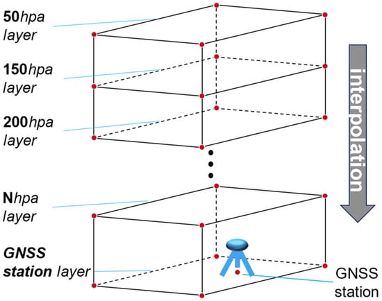
Figure 4.
The schematic diagram for interpolating the interest point’s ZTD.
To ensure the accuracy of the interpolated ZTD at the point of interest, the initial heights of the four corner points must match the height of the point of interest. In this situation, all heights are uniformly converted to geopotential height [50]:
where represents the geopotential height (unit: meters), denotes the potential, and is the gravitational acceleration, taken as 9.80655 m/s2.
For the GNSS station heights, the ellipsoidal heights are first converted to orthometric heights using the EGM2008 model [51,52], and then the orthometric heights are converted to geoidal heights using the following formula. The method for converting orthometric height to geopotential height is as follows:
where denotes the latitude, represents the normal gravity value on the rotating ellipsoid surface, indicates the effective radius of the Earth at latitude , and signifies the normal gravity value on the ellipsoid surface at latitude 45 degrees, which is 9.80655 m/s2. The values of and can be obtained using the following formulas [50]:
Due to the absence of necessary parameters for calculating ZTD in the surface layer of the forecasted meteorological parameters, the parameters for calculating ZTD must be derived from the upper dataset. Additionally, it is required to interpolate the meteorological parameters from the upper layers to the altitude of the point of interest.
For the pressure values, when the altitude of the point of interest is within the height range of the upper-layer data, linear interpolation is used to obtain the interpolated value at the point of interest. When the altitude of the point of interest is lower than the lowest level of the upper layer, the following method is used for interpolation [53]:
where represents the pressure at the interpolation point, is the pressure value at the lowest level in the upper-layer data, and is the absolute height difference between the interpolation point and the lowest level of the upper layer.
For temperature interpolation, if the altitude of the point of interest lies within the altitude range of the upper dataset, the temperature is linearly interpolated based on the height difference between the closest altitude layer and the point of interest. If the altitude of the point of interest is lower than the lowest altitude in the upper dataset, the temperature at the point of interest is calculated using the mean lapse rate derived from the temperatures at 850, 925, and 1000 hPa pressure levels according to the following formula. When the lapse rate exceeds 10 or is negative, a lapse rate of 6.5 is used [45,54].
For specific humidity interpolation, if the altitude of the point of interest falls within the altitude range of the upper dataset, the specific humidity is linearly interpolated between the two nearest layers based on the height difference. If the altitude of the station is lower than the lowest altitude in the upper dataset, the specific humidity at the point of interest is calculated using the humidity lapse rate derived from the specific humidity values at the 850, 925, and 1000 hPa pressure levels.
4. Results
To assess the performance of AI meteorological models in real-time forecasting of tropospheric delay (AI-ZTD), this study conducted an experimental analysis of AI-ZTD from four perspectives. First, the accuracy of the GPT-3, Pangu, and Fengwu models was compared. Second, the impact of seasonal variations on model accuracy was examined. Third, the influence of station altitude on AI-ZTD results was analyzed. Finally, the global accuracy distribution of AI-ZTD was investigated.
In this experiment, the ZTD calculated from the GNSS was used as the reference value (GNSS-ZTD). The GNSS-ZTD data were obtained from the Wuhan University IGS Data Analysis Center, covering the entire year of 2023. After data preprocessing, we selected 81 stations with complete annual data. The distribution of the GNSS stations is in Figure 5:
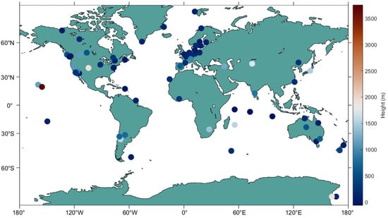
Figure 5.
The schematic map of GNSS station positions where the colors reflect elevation (ellipsoidal height).
4.1. Comparison of Model Accuracies
In this experiment, GNSS-ZTD was used as the primary reference standard. The calculated results of the ERA5, GPT3, Pangu, and Fengwu models were compared with the GNSS-ZTD, and the RMSE values were computed. Both Pangu and Fengwu provide forecast data, and, to facilitate comparison, their forecast intervals were standardized to 6 h. The year 2023 consisted of 365 days, and the data were divided into 72 groups, with each group covering 5 days. The Fengwu and Pangu models use the first day’s data for each group as the background field and perform forecasts at 6 h intervals. Pangu generates 19 forecasts per group, up to midnight on the sixth day, while Fengwu generates 24 forecasts per group, up to midnight on the seventh day. The GPT3 model also calculates ZTD values at the same time points as Pangu, with a 6 h interval from the first day of each group until midnight on the sixth day. In total, 72 groups of data were expected, but, due to missing GNSS-ZTD data on certain days from the IGS center at Wuhan University, 68 groups were available for analysis. The RMSE values at each time point for all 81 GNSS stations across the 68 data groups were compared with the GNSS-ZTD, and the results were plotted.
In Figure 6, the vertical axis represents the RMSE between the ZTD values calculated by the four models and the GNSS-ZTD, while the horizontal axis represents the forecast time, specifically the hours of each day in the group. The Figure 6 indicates that the ZTD calculated by ERA5 had the smallest error compared to the GNSS-ZTD, with RMSE values all below 2 cm. In contrast, the GPT3 model showed the largest ZTD error over 5 days, around 5 cm. The Pangu and Fengwu models demonstrated higher ZTD accuracy in the early stages of forecasting, outperforming the ERA5. However, as the number of forecasts increased, the ZTD errors of both models began to rise, likely due to the cumulative error from using each forecast result as the initial value for the next prediction. In the later stages, Fengwu exhibited better accuracy than Pangu. By the end of the fifth day at 00:00, the ZTD RMSE for Fengwu was 2.30 cm, compared to 2.74 cm for Pangu. Even by the seventh day at 00:00, Fengwu’s predicted ZTD RMSE remained as low as 2.85 cm. Therefore, between the Pangu and Fengwu models, the Fengwu model is recommended for ZTD calculations. It is worth noting that this study utilized the open-source 13-layer version of the Fengwu model. There is also a 37-layer version of the Fengwu model, which may offer even higher accuracy.
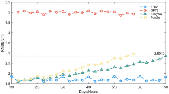
Figure 6.
Time distribution of the median error between ZTD values calculated by the ERA5, GPT3, Fengwu, and Pangu models and the GNSS-ZTD across 68 groups at 81 global stations.
4.2. Seasonal Impact
Previous studies have shown that seasonal variations in meteorological parameters can cause seasonal fluctuations in tropospheric delay [30,45,55,56]. To evaluate the performance of AI-ZTD under different seasonal conditions, this study conducted a monthly analysis comparing AI-ZTD with the GNSS-ZTD. Using GNSS-ZTD as the reference, the error distribution of AI-ZTD across different months was examined. As the accuracy of the Pangu and Fengwu models has already been compared, only the Fengwu model will be used for validation in this section. To avoid the impact of seasonal differences between the Northern and Southern Hemispheres, data from 60 GNSS stations in the Northern Hemisphere were selected for comparison. The error distribution is presented in the form of a box plot, as shown in Figure 7.
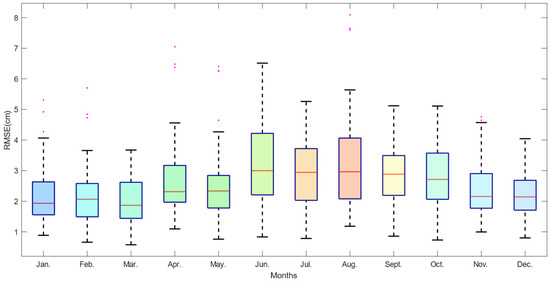
Figure 7.
A box plot of the differences between AI-ZTD and the GNSS-ZTD, with each month’s data represented as a separate group.
Figure 7 shows that the errors of AI-ZTD exhibit significant fluctuations in June, July, and August, while the errors are relatively smaller in winter. This suggests that, in the summer months of the Northern Hemisphere, due to rising temperatures and more complex variations in meteorological parameters, the AI model’s predictions of meteorological parameters become less accurate, leading to fluctuations in the calculated ZTD errors. The median error is highest in June at 3.00 cm and lowest in March at 1.93 cm. Additionally, the upper limit of the error in June is the highest at 6.51 cm, while the lower limit in March is the lowest at 0.57 cm. The average median error over the 12 months is 2.44 cm. These results indicate that AI models may struggle to accurately predict during seasons with highly variable meteorological parameters, which affects the prediction of tropospheric delay parameters. Nevertheless, the AI predictions also demonstrate good stability, with an average median error of 2.44 cm throughout the year.
4.3. Impact of Station Altitude on AI-ZTD
Previous studies have shown that water vapor activity is more frequent near the surface, making it more difficult to predict [57,58]. To analyze the impact of different elevations on AI-ZTD calculations, this study categorizes GNSS stations based on elevation, with classifications in 500-meter intervals. Additionally, the effect of different forecast lead times was analyzed with a 6 h time interval. The GNSS-ZTD values were used as a reference, and histograms of errors were plotted for stations at different altitudes and forecast lead times.
As shown in Figure 8, the RMSE decreases with increasing station elevation, with the largest RMSE observed for stations below 500 m. From some of the water vapor tomography results, it can be seen that water vapor distribution decreases with altitude, which may explain this result [59,60,61]. Therefore, caution is advised when using the AI-ZTD model near low-altitude stations. However, compared to the GNSS-ZTD results, AI-ZTD still demonstrates good accuracy and can serve as a valuable supplement for ZTD calculations in regions lacking observational data.
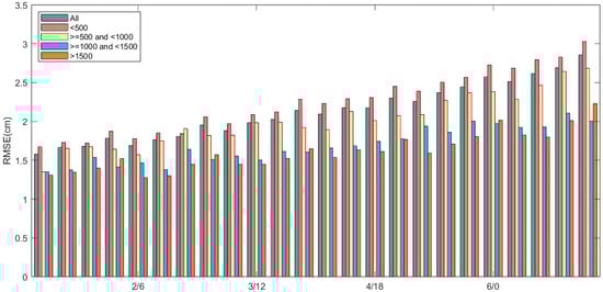
Figure 8.
The RMSE comparison histogram between AI-ZTD and GNSS-ZTD is shown. The data are divided into four height ranges, with the x-axis representing different forecast lead times, and each data group is separated by an interval of 6 h. Height units: meters.
Furthermore, this study also analyzed the impact of different forecast lead times. The figure shows that, as the forecast lead time increases, the accuracy AI-ZTD accuracy decreases with increasing forecast duration, with RMSE values rising across stations at different elevations. Within the first three days, the accuracy of AI-ZTD is better than 2 cm, and at 00:00 on the seventh day, the RMS value of AI-ZTD compared to the GNSS-ZTD remains below 3 cm. This indicates that, as the forecast lead time increases, the prediction error of AI-ZTD also gradually increases.
4.4. Global Accuracy of AI-ZTD
To further analyze the global applicability of AI-ZTD, AI-ZTD data for the entire year of 2023 were compared with GNSS-ZTD data, and the global distribution of residuals was plotted. The AI-ZTD data correspond to the predicted values for the sixth day, which were compared with the GNSS-ZTD. The RMSE was calculated for each station over the year. A total of 81 stations were selected globally, and the overall RMSE distribution is shown in the Figure 9.
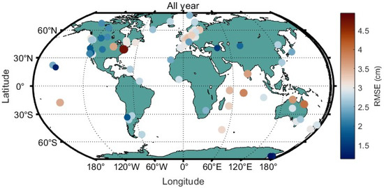
Figure 9.
RMSE distribution of the comparison between AI-ZTD and GNSS-ZTD at 81 global stations.
As shown in Figure 9, the ZTD provided by AI-ZTD demonstrates a relatively uniform accuracy distribution globally. The RMSE distribution of the ZTD over the entire year shows good consistency between AI-ZTD and the GNSS-ZTD. However, due to the sparse distribution of stations, the overall global distribution is not very clear. To further analyze the data, we compared AI-ZTD with ERA5 data, using data from the entire year of 2023. The prediction period of AI-ZTD is 6 days, and 60 time points were selected from ERA5 data. Layered data were used, and the ZTD was calculated using the integration formula introduced earlier. The grid resolution was set to 1° × 1°, and, based on 60 data points throughout the year, the RMSE distribution of the residuals between AI-ZTD and ERA5’s ZTD was plotted, as shown in Figure 10:
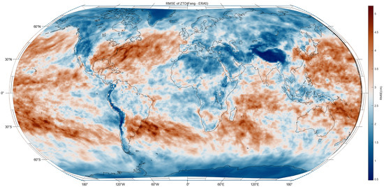
Figure 10.
Global RMSE distribution of the comparison between AI-ZTD and ERA5’s ZTD at a 1° × 1° resolution.
Figure 10 demonstrates a high degree of consistency between AI-ZTD and the ERA5-ZTD across most global regions. In the majority of areas, the RMSE distribution is within a blue range, indicating a minimal error, generally less than 2.5 cm. However, larger errors are observed over oceanic regions compared to land areas, particularly in transition zones from ocean to land near the equator, where tropical storms and hurricanes frequently occur [62]. In contrast, the Tibetan Plateau shows a minimal discrepancy between AI-ZTD and ERA5-ZTD, aligning with our earlier findings related to station elevation. Several factors likely contribute to the larger errors over oceans. Firstly, the lack of reliable oceanic observations results in lower model accuracy. The AI meteorological models are trained on reanalysis datasets, which are influenced by the quality of the original data, leading to potential accuracy limitations. Secondly, meteorological variability is more complex near the equator, making accurate prediction more challenging as the accuracy of AI weather models is likely to correlate with the precision of ERA5 data. It is advisable to exercise caution when applying AI models in regions with larger discrepancies. Further research is essential to develop models better suited for these areas.
5. Discussion
This study presents an extensive evaluation of the AI meteorological models’ ability to predict ZTD using data from GNSS stations. The results show that AI models like Fengwu and Pangu demonstrate significant potential in this domain, with Fengwu outperforming Pangu in long-term forecasts, maintaining a lower RMSE even after several days.
The seasonal analysis revealed that AI-ZTD accuracy decreases during summer months in the Northern Hemisphere, likely due to the increased complexity of meteorological parameters during warmer seasons. In contrast, polar regions exhibit relatively lower errors, likely influenced by lower temperatures and water vapor content.
The impact of elevation on ZTD forecasting is also evident, with stations at lower elevations showing lower forecast accuracy compared to those at higher elevations. This difference may be related to the vertical distribution of water vapor. Therefore, caution is needed when using AI meteorological models at low-elevation stations.
Nevertheless, despite the overall strong performance, certain limitations are observed. For example, AI-ZTD shows greater discrepancies over oceanic regions and areas frequently affected by typhoons and hurricanes. This is largely due to the lack of observational data over oceans and the complex climatic dynamics in these regions. These issues underscore the need for caution when applying AI models in these areas, as well as the necessity for further research to refine the models and enhance their applicability in such challenging environments.
Overall, while AI-based ZTD models show great promise, especially in their computational efficiency and forecast skill, improvements are needed in handling regions with sparse observational data and complex climate conditions. Further development and refinement of these models will enhance their global applicability and forecast accuracy.
Author Contributions
The paper was conceived by S.X. and J.M., with the methodology proposed by S.X. and X.X. The program was developed by S.X. and J.M., validation was completed by Z.S., the data were collected and organized by L.H. and the manuscript was written by S.X. All authors have read and agreed to the published version of the manuscript.
Funding
This research was supported by the Guiding Project of the Scientific Research Plan of the Hubei Provincial Department of Education (no. B2023172), the Fund of the Guangxi Key Laboratory of Spatial Information and Measurement (no. 21-238-21-15), the Doctoral Startup Fund Project of Hubei University of Science and Technology (no. BK202405), and the National Natural Science Foundation of China General Project “Fine Correction of Global Tropospheric Delay Effect Based on Non-Uniform Grid Parameterization and Its Application” (no. 42474057).
Institutional Review Board Statement
Not applicable.
Informed Consent Statement
Not applicable.
Data Availability Statement
The ERA5 data are available at https://cds.climate.copernicus.eu/datasets/reanalysis-era5-single-levels?tab=overview (accessed on 13 October 2024) and https://cds.climate.copernicus.eu/datasets/reanalysis-era5-pressure-levels?tab=overview(accessed on 13 October 2024). The IGS data are available via FTP at ftp://igs.gnsswhu.cn/ (accessed on 13 October 2024). The IGS station location information is available at https://network.igs.org/ (accessed on 13 October 2024). The Fengwu model is available at https://github.com/OpenEarthLab/FengWu (accessed on 13 October 2024). The Pangu model is available at https://github.com/198808xc/Pangu-Weather (accessed on 13 October 2024).
Acknowledgments
The authors would like to thank the ECMWF for providing ERA5 data. We also would like to thank the International GNSS Service for providing the ZTD data used in this study. We also extend our gratitude to the Vienna Mapping Functions Open Access Data project team for providing the GPT3 model, to Huawei for providing the Pangu model, and to the Shanghai Artificial Intelligence Laboratory for providing the Fengwu model.
Conflicts of Interest
The authors declare no conflicts of interest.
References
- Eriksson, D.; MacMillan, D.S.; Gipson, J.M. Tropospheric delay ray tracing applied in VLBI analysis. J. Geophys. Res. Solid Earth 2014, 119, 9156–9170. [Google Scholar] [CrossRef]
- Mendes, V.B.; Prates, G.; Pavlis, E.C.; Pavlis, D.E.; Langley, R.B. Improved Mapping Functions for Atmospheric Refraction Correction in SLR. Geophys. Res. Lett. 2002, 29, 53-1-53-4. [Google Scholar] [CrossRef]
- Lu, C.; Zus, F.; Ge, M.; Heinkelmann, R.; Dick, G.; Wickert, J.; Schuh, H. Tropospheric Delay Parameters from Numerical Weather Models for Multi-GNSS Precise Positioning. Atmos. Meas. Tech. 2016, 9, 5965–5973. [Google Scholar] [CrossRef]
- Kinoshita, Y.; Shimada, M.; Furuya, M. InSAR Observation and Numerical Modeling of the Water Vapor Signal during a Heavy Rain: A Case Study of the 2008 Seino Event, Central Japan. Geophys. Res. Lett. 2013, 40, 4740–4744. [Google Scholar] [CrossRef]
- Huang, L.; Pan, A.; Chen, F.; Guo, F.; Li, H.; Liu, L. A Novel Global Grid Model for Soil Moisture Retrieval Considering Geographical Disparity in Spaceborne GNSS-R. Satell. Navig. 2024, 5, 29. [Google Scholar] [CrossRef]
- Bevis, M.; Businger, S.; Herring, T.A.; Rocken, C.; Anthes, R.A.; Ware, R.H. Gps Meteorology—Remote-Sensing of Atmospheric Water-Vapor Using the Global Positioning System. J. Geophys. Res.-Atmos. 1992, 97, 15787–15801. [Google Scholar] [CrossRef]
- Gurbuz, G.; Jin, S. Long-time Variations of Precipitable Water Vapour Estimated from GPS, MODIS and Radiosonde Observations in Turkey. Int. J. Climatol. 2017, 37, 5170–5180. [Google Scholar] [CrossRef]
- Teke, K.; Nilsson, T.; Böhm, J.; Hobiger, T.; Steigenberger, P.; García-Espada, S.; Haas, R.; Willis, P. Troposphere Delays from Space Geodetic Techniques, Water Vapor Radiometers, and Numerical Weather Models over a Series of Continuous VLBI Campaigns. J. Geod. 2013, 87, 981–1001. [Google Scholar] [CrossRef]
- Toth, C.; Jóźków, G. Remote Sensing Platforms and Sensors: A Survey. ISPRS J. Photogramm. Remote Sens. 2016, 115, 22–36. [Google Scholar] [CrossRef]
- Gutman, S.I.; Benjamin, S.G. The Role of Ground-Based GPS Meteorological Observations in Numerical Weather Prediction. GPS Solut. 2001, 4, 16–24. [Google Scholar] [CrossRef]
- Leandro, R.; Santos, M.; Langley, R.B. UNB Neutral Atmosphere Models: Development and Performance. In Proceedings of the 2006 National Technical Meeting of the Institute of Navigation, Monterey, CA, USA, 18–20 January 2006. [Google Scholar]
- Leandro, R.F.; Langley, R.B.; Santos, M.C. UNB3m_pack: A Neutral Atmosphere Delay Package for Radiometric Space Techniques. GPS Solut. 2008, 12, 65–70. [Google Scholar] [CrossRef]
- Yao, Y.; Hu, Y.; Yu, C.; Zhang, B.; Guo, J. An Improved Global Zenith Tropospheric Delay Model GZTD2 Considering Diurnal Variations. Nonlinear Process. Geophys. 2016, 23, 127–136. [Google Scholar] [CrossRef]
- Li, W.; Yuan, Y.; Ou, J.; He, Y. IGGtrop_SH and IGGtrop_rH: Two Improved Empirical Tropospheric Delay Models Based on Vertical Reduction Functions. IEEE Trans. Geosci. Remote Sens. 2018, 56, 5276–5288. [Google Scholar] [CrossRef]
- Zhu, G.; Huang, L.; Yang, Y.; Li, J.; Zhou, L.; Liu, L. Refining the ERA5-Based Global Model for Vertical Adjustment of Zenith Tropospheric Delay. Satell. Navig. 2022, 3, 27. [Google Scholar] [CrossRef]
- Huang, L.; Zhu, G.; Liu, L.L.; Chen, H.; Jiang, W.P. A Global Grid Model for the Correction of the Vertical Zenith Total Delay Based on a Sliding Window Algorithm. GPS Solut. 2021, 25, 14. [Google Scholar] [CrossRef]
- Song, S.; Zhu, W.; Chen, Q.; Liou, Y. Establishment of a New Tropospheric Delay Correction Model over China Area. Sci. China Phys. Mech. Astron. 2011, 54, 2271–2283. [Google Scholar] [CrossRef]
- Penna, N.; Dodson, A.; Chen, W. Assessment of EGNOS Tropospheric Correction Model. J. Navig. 2001, 54, 37–55. [Google Scholar] [CrossRef]
- Ding, M.; Ding, J.; Peng, Z.; Su, M.; Sun, T. Developments of Empirical Models for Vertical Adjustment of Precipitable Water Vapor Measured by GNSS. Adv. Space Res. 2024. [Google Scholar] [CrossRef]
- Huang, L.; Lan, S.; Zhu, G.; Chen, F.; Li, J.; Liu, L. A Global Grid Model for the Estimation of Zenith Tropospheric Delay Considering the Variations at Different Altitudes. Geosci. Model Dev. Discuss. 2023, 2023, 1–18. [Google Scholar] [CrossRef]
- Huang, L.; Zhu, G.; Peng, H.; Liu, L.; Ren, C.; Jiang, W. An Improved Global Grid Model for Calibrating Zenith Tropospheric Delay for GNSS Applications. GPS Solut. 2023, 27, 17. [Google Scholar] [CrossRef]
- Boehm, J.; Heinkelmann, R.; Schuh, H. Short Note: A Global Model of Pressure and Temperature for Geodetic Applications. J. Geod. 2007, 81, 679–683. [Google Scholar] [CrossRef]
- Böhm, J.; Möller, G.; Schindelegger, M.; Pain, G.; Weber, R. Development of an Improved Empirical Model for Slant Delays in the Troposphere (GPT2w). GPS Solut. 2015, 19, 433–441. [Google Scholar] [CrossRef]
- Landskron, D.; Böhm, J. VMF3/GPT3: Refined Discrete and Empirical Troposphere Mapping Functions. J. Geod. 2018, 92, 349–360. [Google Scholar] [CrossRef]
- Lagler, K.; Schindelegger, M.; Böhm, J.; Krásná, H.; Nilsson, T. GPT2: Empirical Slant Delay Model for Radio Space Geodetic Techniques. Geophys. Res. Lett. 2013, 40, 1069–1073. [Google Scholar] [CrossRef]
- Hopfield, H.S. Tropospheric Effect on Electromagnetically Measured Range: Prediction from Surface Weather Data. Radio Sci. 1971, 6, 357–367. [Google Scholar] [CrossRef]
- Saastamoinen, J. Contributions to the Theory of Atmospheric Refraction. Bull. Géod. 1972, 105, 279–298. [Google Scholar] [CrossRef]
- Black, H.D. An Easily Implemented Algorithm for the Tropospheric Range Correction. J. Geophys. Res. Solid Earth 1978, 83, 1825–1828. [Google Scholar] [CrossRef]
- Huang, L.; Wang, X.; Xiong, S.; Li, J.; Liu, L.; Mo, Z.; Fu, B.; He, H. High-Precision GNSS PWV Retrieval Using Dense GNSS Sites and in-Situ Meteorological Observations for the Evaluation of MERRA-2 and ERA5 Reanalysis Products over China. Atmos. Res. 2022, 276, 106247. [Google Scholar] [CrossRef]
- Chen, B.; Yu, W.; Wang, W.; Zhang, Z.; Dai, W. A Global Assessment of Precipitable Water Vapor Derived from GNSS Zenith Tropospheric Delays with ERA5, NCEP FNL, and NCEP GFS Products. Earth Space Sci. 2021, 8, e2021EA001796. [Google Scholar] [CrossRef]
- Cao, L.; Zhang, B.; Li, J.; Yao, Y.; Liu, L.; Ran, Q.; Xiong, Z. A Regional Model for Predicting Tropospheric Delay and Weighted Mean Temperature in China Based on GRAPES_MESO Forecasting Products. Remote Sens. 2021, 13, 2644. [Google Scholar] [CrossRef]
- Chen, K.; Han, T.; Gong, J.; Bai, L.; Ling, F.; Luo, J.-J.; Chen, X.; Ma, L.; Zhang, T.; Su, R.; et al. FengWu: Pushing the Skillful Global Medium-Range Weather Forecast beyond 10 Days Lead. arXiv 2023, arXiv:2304.02948. [Google Scholar]
- Bi, K.; Xie, L.; Zhang, H.; Chen, X.; Gu, X.; Tian, Q. Accurate Medium-Range Global Weather Forecasting with 3D Neural Networks. Nature 2023, 619, 533–538. [Google Scholar] [CrossRef] [PubMed]
- Lam, R.; Sanchez-Gonzalez, A.; Willson, M.; Wirnsberger, P.; Fortunato, M.; Alet, F.; Ravuri, S.; Ewalds, T.; Eaton-Rosen, Z.; Hu, W.; et al. Learning Skillful Medium-Range Global Weather Forecasting. Science 2023, 382, 1416–1421. [Google Scholar] [CrossRef]
- Chen, L.; Zhong, X.; Zhang, F.; Cheng, Y.; Xu, Y.; Qi, Y.; Li, H. FuXi: A Cascade Machine Learning Forecasting System for 15-Day Global Weather Forecast. NPJ Clim. Atmos. Sci. 2023, 6, 190. [Google Scholar] [CrossRef]
- Bi, H.; Huang, L.; Zhang, H.; Xie, S.; Zhou, L.; Liu, L. A Deep Learning-Based Model for Tropospheric Wet Delay Prediction Based on Multi-Layer 1D Convolution Neural Network. Adv. Space Res. 2024, 73, 5031–5042. [Google Scholar] [CrossRef]
- Lu, C.; Zheng, Y.; Wu, Z.; Zhang, Y.; Wang, Q.; Wang, Z.; Liu, Y.; Zhong, Y. TropNet: A Deep Spatiotemporal Neural Network for Tropospheric Delay Modeling and Forecasting. J. Geod. 2023, 97, 34. [Google Scholar] [CrossRef]
- Schultz, M.G.; Betancourt, C.; Gong, B.; Kleinert, F.; Langguth, M.; Leufen, L.H.; Mozaffari, A.; Stadtler, S. Can Deep Learning Beat Numerical Weather Prediction? Phil. Trans. R. Soc. A 2021, 379, 20200097. [Google Scholar] [CrossRef]
- Charlton-Perez, A.J.; Dacre, H.F.; Driscoll, S.; Gray, S.L.; Harvey, B.; Harvey, N.J.; Hunt, K.M.R.; Lee, R.W.; Swaminathan, R.; Vandaele, R.; et al. Do AI Models Produce Better Weather Forecasts than Physics-Based Models? A Quantitative Evaluation Case Study of Storm Ciarán. NPJ Clim. Atmos. Sci. 2024, 7, 93. [Google Scholar] [CrossRef]
- Pathak, J.; Subramanian, S.; Harrington, P.; Raja, S.; Chattopadhyay, A.; Mardani, M.; Kurth, T.; Hall, D.; Li, Z.; Azizzadenesheli, K.; et al. FourCastNet: A Global Data-Driven High-Resolution Weather Model Using Adaptive Fourier Neural Operators. arXiv 2022, arXiv:2202.11214. [Google Scholar]
- Bi, K.; Xie, L.; Zhang, H.; Chen, X.; Gu, X.; Tian, Q. Pangu-Weather: A 3D High-Resolution Model for Fast and Accurate Global Weather Forecast. arXiv 2022, arXiv:2211.02556. [Google Scholar]
- Xu, H.; Zhao, Y.; Zhao, D.; Duan, Y.; Xu, X. Improvement of Disastrous Extreme Precipitation Forecasting in North China by Pangu-Weather AI-Driven Regional WRF Model. Environ. Res. Lett. 2024, 19, 54051. [Google Scholar] [CrossRef]
- Vázquez, B.G.E.; Grejner-Brzezinska, D.A. GPS-PWV estimation and validation with radiosonde data and numerical weather prediction model in Antarctica. GPS Solut. 2012, 17, 29–39. [Google Scholar] [CrossRef]
- Sun, P.; Zhang, K.; Wu, S.; Wang, R.; Zhu, D.; Li, L. An Investigation of a Voxel-Based Atmospheric Pressure and Temperature Model. GPS Solut. 2023, 27, 56. [Google Scholar] [CrossRef]
- Huang, L.; Guo, L.; Liu, L.; Chen, H.; Chen, J.; Xie, S. Evaluation of the ZWD/ZTD Values Derived from MERRA-2 Global Reanalysis Products Using GNSS Observations and Radiosonde Data. Sensors 2020, 20, 6440. [Google Scholar] [CrossRef]
- Chen, B.; Liu, Z. A Comprehensive Evaluation and Analysis of the Performance of Multiple Tropospheric Models in China Region. IEEE Trans. Geosci. Remote Sens. 2016, 54, 663–678. [Google Scholar] [CrossRef]
- Rüeger, J.M. Refractive Index Formulae for Radio Waves. In Proceedings of the FIG XXII International Congress, Washington, DC, USA, 19–26 April 2002. [Google Scholar]
- Mendes, V. Modeling the Neutral-Atmospheric Propagation Delay in Radiometric Space Techniques. Ph.D. Dissertation, University of New Brunswick, Fredericton, NB, Canada, 1999. [Google Scholar]
- Wallace, J.M. Atmospheric Science: An Introductory Survey; Elsevier: Berkeley, CA, USA, 2006; ISBN 978-0-12-732951-2. [Google Scholar]
- Dousa, J.; Elias, M. An Improved Model for Calculating Tropospheric Wet Delay. Geophys. Res. Lett. 2014, 41, 4389–4397. [Google Scholar] [CrossRef]
- Pavlis, N.K.; Holmes, S.A.; Kenyon, S.C.; Factor, J.K. The Development and Evaluation of the Earth Gravitational Model 2008 (EGM2008). J. Geophys. Res. Solid Earth 2012, 117, B4. [Google Scholar] [CrossRef]
- The EGM2008 Global Gravitational Model. Available online: https://ui.adsabs.harvard.edu/abs/2008AGUFM.G22A..01P/abstract (accessed on 13 October 2024).
- Liu, L.; Yao, C.; Xiong, S.; Huang, L. Research on GPS Inversion of Atmospheric Precipitable Water Based on In-terpolated Atmospheric Pressure. Geod. Geodyn. 2013, 33, 72–78. [Google Scholar] [CrossRef]
- Wang, X.; Zhang, K.; Wu, S.; Fan, S.; Cheng, Y. Water Vapor-Weighted Mean Temperature and Its Impact on the Determination of Precipitable Water Vapor and Its Linear Trend. J. Geophys. Res.-Atmos. 2016, 121, 833–852. [Google Scholar] [CrossRef]
- Hadas, T.; Hobiger, T.; Hordyniec, P. Considering Different Recent Advancements in GNSS on Real-Time Zenith Troposphere Estimates. GPS Solut. 2020, 24, 99. [Google Scholar] [CrossRef]
- Sun, J.; Wu, Z.; Yin, Z.; Ma, B. A Simplified GNSS Tropospheric Delay Model Based on the Nonlinear Hypothesis. GPS Solut. 2017, 21, 1735–1745. [Google Scholar] [CrossRef]
- Zhao, Q.; Yao, Y.; Cao, X.; Zhou, F.; Xia, P. An Optimal Tropospheric Tomography Method Based on the Multi-GNSS Observations. Remote Sens. 2018, 10, 234. [Google Scholar] [CrossRef]
- Zhao, Q.; Yao, W.; Yao, Y.; Li, X. An improved GNSS tropospheric tomography method with the GPT2w model. GPS Solut. 2020, 24, 60. [Google Scholar] [CrossRef]
- Xia, P.; Peng, W.; Yuan, P.; Ye, S. Monitoring Urban Heat Island Intensity Based on GNSS Tomography Technique. J. Geod. 2024, 98, 1. [Google Scholar] [CrossRef]
- Zhang, W.; Zhang, S.; Moeller, G.; Qi, M.; Ding, N. An Adaptive-Degree Layered Function-Based Method to GNSS Tropospheric Tomography. GPS Solut. 2023, 27, 67. [Google Scholar] [CrossRef]
- Ding, N.; Tan, X.; Liu, X.; He, Z.; Zhang, Y.; Wang, Y.; Zhang, S.; Holden, L.; Zhang, K. Adaptive Voxel-Based Model for the Dynamic Determination of Tomographic Region. Remote Sens. 2023, 15, 492. [Google Scholar] [CrossRef]
- Jing, R.; Heft-Neal, S.; Chavas, D.R.; Griswold, M.; Wang, Z.; Clark-Ginsberg, A.; Guha-Sapir, D.; Bendavid, E.; Wagner, Z. Global Population Profile of Tropical Cyclone Exposure from 2002 to 2019. Nature 2024, 626, 549–554. [Google Scholar] [CrossRef]
Disclaimer/Publisher’s Note: The statements, opinions and data contained in all publications are solely those of the individual author(s) and contributor(s) and not of MDPI and/or the editor(s). MDPI and/or the editor(s) disclaim responsibility for any injury to people or property resulting from any ideas, methods, instructions or products referred to in the content. |
© 2024 by the authors. Licensee MDPI, Basel, Switzerland. This article is an open access article distributed under the terms and conditions of the Creative Commons Attribution (CC BY) license (https://creativecommons.org/licenses/by/4.0/).