Building Change Detection Network Based on Multilevel Geometric Representation Optimization Using Frame Fields

Abstract

To address the challenges of accurately segmenting irregular building boundaries in complex urban environments faced by existing remote sensing change detection methods, this paper proposes a building change detection network based on multilevel geometric representation optimization using frame fields called BuildingCDNet. The proposed method employs a multi-scale feature aggregation encoder–decoder architecture, leveraging contextual information to capture the characteristics of buildings of varying sizes in the imagery. Cross-attention mechanisms are incorporated to enhance the feature correlations between the change pairs. Additionally, the frame field is introduced into the network to model the complex geometric structure of the building target. By learning the local orientation information of the building structure, the frame field can effectively capture the geometric features of complex building features. During the training process, a multi-task learning strategy is used to align the predicted frame field with the real building outline, while learning the overall segmentation, edge outline, and corner point features of the building. This improves the accuracy of the building polygon representation. Furthermore, a discriminative loss function is constructed through multi-task learning to optimize the polygonal structured information of the building targets. The proposed method achieves state-of-the-art results on two commonly used datasets.

1. Introduction

In satellite remote sensing change detection tasks, analyzing satellite images from different time periods to detect changes in surface objects or areas has become an essential tool in fields such as environmental monitoring [1,2,3,4], disaster assessment [5,6,7], and land use/cover change studies [8,9,10,11,12]. With the rapid advancement of remote sensing technology, satellite sensors can now provide higher spatial and temporal resolution image data, enabling a more precise analysis of surface details [13,14]. Building change detection, a critical subfield of satellite remote sensing change detection, focuses on identifying changes such as new construction, demolition, or expansion of buildings by comparing satellite images from different times [15,16]. This task has wide applications in urban planning, post-disaster reconstruction, and monitoring of illegal structures. As urbanization accelerates, the importance of building change detection in geographic information systems (GISs) and remote sensing surveillance continues to grow [17,18]. High-resolution remote sensing images can greatly improve the efficiency and accuracy of automated monitoring of dynamic urban changes [19,20,21].

Similarly to typical binary change detection tasks, building change detection generally involves determining whether building targets have changed or remained unchanged [22,23]. Traditional methods for building change detection often include differencing techniques, such as directly or indirectly comparing image differences or logs; classification methods, which classify or extract building locations from pre- and post-change images and then compare them across time; and other approaches such as change vector analysis, PCA, and Markov random fields [24,25,26]. There are also feature transfer-based methods [27], which rely on various statistical rules or high-dimensional modeling to facilitate the comparison of pre- and post-change images in a new feature space or under specific measurement rules, thus obtaining change detection results.

In recent years, with the development of deep learning technology, convolutional neural network (CNN)-based change detection methods have gradually become mainstream [28]. Compared with traditional methods, deep learning significantly improves the accuracy of building change detection by automatically learning features. The Unet network, originally designed for medical image segmentation, has been widely applied to building change detection due to its outstanding performance. Its symmetrical encoder–decoder structure effectively combines contextual information with precise location details, providing robust support for identifying change regions [29,30]. However, Unet still faces certain limitations when handling multi-scale targets, particularly in detecting small objects. To address this issue, researchers have started incorporating attention mechanisms into change detection models. Attention mechanisms allow models to focus more on important regions within the image, thus enhancing the accuracy of detecting small objects. For instance, by introducing channel attention and spatial attention, models can better focus on features related to building changes, significantly improving detection accuracy. The integration of a residual network (ResNet) addresses the vanishing gradient problem in training deep neural networks due to its residual structure, enabling deeper feature learning. In change detection tasks, the use of ResNet not only enhances feature extraction but also improves the model’s ability to capture subtle changes [31,32]. Transformer, a novel network architecture, introduces a self-attention mechanism that effectively handles long-range dependencies, offering new perspectives for building change detection. By leveraging Transformer, models can better capture global information in images, leading to superior performance in change detection [33,34]. Recently, the Mamba technique, a deep learning approach based on state–space models (SSMs), has also been applied to change detection tasks due to its efficient computational capabilities and long-sequence modeling capacity [35].

Despite these advancements, building change detection still faces many challenges. First, buildings in remote sensing images often exhibit complex edge features, and the presence of other objects, such as roads, can lead to false detections and missed detections. Second, the scale of building change regions is often small relative to the whole image, resulting in a class imbalance problem that causes models to bias towards unchanged regions. Additionally, most methods adopt generalized change detection strategies, without fully leveraging the unique characteristics of building targets.

To address these challenges, this paper proposes a building change detection network optimized for multilevel geometric representation using frame fields, with the following innovations:

(1) Introduction of Frame Fields into Building Change Detection: For the first time, frame fields are applied to the task of building change detection, enabling comprehensive geometric modeling of buildings’ segmentation, edge contours, and corner features. Compared with traditional methods, this approach not only captures the global geometric characteristics of buildings more accurately but also finely depicts local details. Frame fields are particularly effective in complex urban environments where buildings exhibit diverse shapes and intricate contours, precisely modeling changes in building corners and edges. Additionally, by incorporating a multi-scale feature aggregation encoder–decoder module and cross-attention mechanism, the model’s adaptability and accuracy in expressing the geometric features of complex building shapes are significantly enhanced.

(2) Multi-Task Learning Strategy: The proposed method adopts a multi-task learning strategy to jointly optimize building segmentation, edge extraction, and corner detection tasks, thereby enhancing the polygonal geometric representation of buildings. By leveraging the synergy between different tasks, the model improves its understanding of building details. To further enhance the accuracy of building segmentation and contour extraction, an innovative loss function is designed, targeting the geometric features of buildings. This composite loss function integrates factors such as segmentation accuracy, edge alignment, and frame field directional smoothness. As a result, the network simultaneously considers both the global segmentation of buildings and local geometric features, producing more regular and precise polygonal building contours. This design not only improves the overall accuracy of building segmentation but also reduces issues such as irregular edges and geometric distortions, with particularly strong performance in urban scenes with complex building structures.

The remainder of this paper is organized as follows: Section 2 reviews related work. Section 3 describes the workflow of the proposed building change detection network based on frame field multilevel geometric representation optimization. Section 4 presents the experimental results and ablation studies on various datasets. Section 5 discusses computation costs and parametric analysis. Finally, Section 6 concludes the paper and discusses future directions.

2. Related Works

2.1. Non-Deep Learning Change Detection Methods

For traditional non-deep learning change detection methods, differencing techniques primarily detect changes by comparing images captured at different time points. These methods aim to highlight the areas of change in the images to facilitate further analysis. They are simple to implement and computationally inexpensive, but they are highly sensitive to variations in lighting, noise, and image registration errors, often resulting in false positives or missed detections.

Classification-based methods classify the pre- and post-change images separately, extracting the precise locations of buildings, and then compare the classification results from both time periods to determine whether changes have occurred [36,37]. Peng et al. [38] proposed an object-based change detection method for high-resolution remote sensing images (OBCD), which integrates segmentation optimization with multi-feature fusion. Additionally, Jian et al. [39] developed a one-class classification (OCC) technique based on generative adversarial networks (GANs) for change detection in time-series remote sensing images. These methods rely heavily on the accuracy of image classification results; if the classification precision is low, it can lead to error accumulation in subsequent change detection steps.

Some other approaches incorporate techniques such as change vector analysis (CVA) to model and compare multi-dimensional features [40,41]. In these methods, image data from before and after the change are mapped and modeled in a feature space, and changes are detected by measuring vector differences in this new feature space, thereby improving the robustness of change detection [42,43]. Our previous research [44] proposed a change vector analysis method based on an adaptive weighted Gaussian mixture model (CVA-AWGMM), where clustering information from a large set of unlabeled samples was used to complement the supervised training information from a few labeled samples. The Gaussian mixture model was employed to fit the distribution of different types of change pixels, obtaining distinct change attributes for each pixel. Li et al. [45] combined fuzzy C-means (FCM) and a cautious Bayesian network (CSBN) with the change vector analysis in a posterior probability space (CVAPS), achieving promising results.

Another common approach is based on principal component analysis (PCA), which reduces the dimensionality of the data to extract key change information. These methods effectively lower the data complexity and highlight essential information for change detection [46]. Conditional random fields (CRFs) are another graph-based technique that models the spatial relationships between buildings and their surroundings. By establishing dependencies between pixels or regions, CRFs help integrate contextual information into the change detection process, reducing the impact of noise. Sun et al. [47] proposed an unsupervised change detection method based on iterative structure transformation and conditional random fields (IST-CRFs). This method combines structure transformation, which is invariant to imaging modalities, with a random field framework to propagate information iteratively and obtain the optimal change map within a global probabilistic model.

In addition, feature transfer methods aim to map multi-temporal image features into a common feature space, making change detection more straightforward. For example, IJGLT (Iterative Joint Global–Local Translation) [48] is an unsupervised change detection method based on transfer learning. It jointly utilizes global and local characteristics of the data and iteratively refines an initial change map to obtain the final detection result. Max Mignotte [49] developed an approach that combines improved geometric fractal decomposition and contraction mapping, followed by unsupervised Bayesian binarization of the pixel difference map between two images. This method projects the pre- and post-change images into a new space for comparison and analysis. However, many of these methods are designed for tiny datasets, and their applicability to large-scale and more complex scenarios remains limited.

2.2. Deep Learning Change Detection Methods

With the rapid advancement of artificial intelligence and the increasing availability of computational resources, the application of deep learning-based change detection methods has become more widespread. Below is an overview of the development in this field.

Daudt et al. [50] were the first to apply fully convolutional Siamese networks to the change detection task for remote sensing images, introducing three important frameworks: fully convolutional early fusion (FC-EF), fully convolutional Siamese concatenation (FC-Siam-conc), and fully convolutional Siamese difference (FC-Siam-diff). These frameworks laid a solid foundation for subsequent research in this domain. STANet [51] leveraged a pyramid attention mechanism to mitigate errors at object boundaries caused by potential misalignment in pixel-wise registration between two temporal images. IFNet [52] adopted a fully convolutional dual-stream architecture to extract highly representative deep features from bi-temporal images. It then used an attention module to fuse multilevel deep features and image difference features for the generation of the change map. Ding et al. [53] applied a variant of the segment anything model (SAM), called FastSAM, to the change detection task, incorporating a convolutional adapter to leverage the visual recognition capabilities of Vision Foundation Models (VFMs) for change detection. Du et al. [54] used convolutional neural networks (CNNs) to extract deep features from imprecisely registered images and automatically matched and extracted common regions. These regions were used as inputs for a support expansion strategy, combined with channel attention to generate training data for a generative adversarial network (GAN). The generator of the GAN then produced optimized images, which were compared to generate the change map. The hierarchical attention network (HANet) [55] employed a progressive foreground-balanced sampling strategy that did not add change information, helping the network learn change pixel features accurately during early training stages, thereby improving detection performance.

In the application of transformer-based structures, BIT [56] is one of the most classic and widely used studies. It represents bi-temporal images as multiple tokens and models spatial–temporal features. The learned context-enriched tokens are then projected back into pixel space through a transformer decoder to refine the original features. Ma et al. [57] proposed BTNIFormer, which integrates a sparse attention mechanism called dilated neighborhood attention (DiNA), where the attention scope for each pixel is confined to its adjacent context, reducing computational complexity. Wang et al. [58] introduced the interactive feature transformer network with spatial detail enhancement module (IFTSDNet), utilizing transformers to capture long-range context while leveraging CNNs for local information extraction. They also designed a spatial detail enhancement module (SDEM) with different receptive fields to refine spatial features, demonstrating the effectiveness of the proposed approach.

ChangeMamba [35] was the first to explore the potential of the Mamba architecture in remote sensing change detection (CD) tasks. It employed the state-of-the-art visual Mamba architecture as the encoder, allowing it to fully learn global spatial context from input images. Three spatial–temporal relationship modeling mechanisms were proposed, naturally integrating with the Mamba architecture to enable spatial–temporal interaction between the multi-temporal features, thereby accurately capturing change information.

Recent studies have also focused on architectural characteristics in change detection. Wang et al. [59] addressed the interference caused by varying perspectives, particularly for objects with height, like buildings. They used cross-temporal stereo matching to obtain elevation data for buildings and corrected dual-temporal digital surface models (DSMs) to detect building changes. Zhang et al. [60] proposed an attention-guided edge refinement network (AERNet), which uses an attention-guided edge refinement network to correct changes in building targets. They also designed a new adaptive weighted binary cross-entropy (SWBCE) loss function, combined with deep supervision (DS) strategies. Iterative edge enhancing framework (IEEF) [21] mitigated difficulties in detecting building edges by densely implementing a detail semantic enhancement module (DSEM) in the decoder section. This module explicitly represents building edge information using difference features between adjacent scales. However, these studies still face challenges related to the incomplete utilization of building-specific characteristics.

3. Materials and Methods

This paper presents a building change detection network, BuildingCDNet, based on frame fields, designed to address challenges such as irregular boundaries and complex shapes of buildings in urban environments. The basic framework of change detection tasks and the overall architecture of BuildingCDNet are first outlined. Then, detailed descriptions are provided for key components, including the multi-scale feature aggregation encoder–decoder module, cross-attention mechanism, frame field, and multi-task learning loss.

3.1. Overall Network Architecture

For building change detection, let $I_1,I_2\in {ℝ}^{H\times W\times 3}$ represent two RGB satellite optical remote sensing images taken at different times before and after the change, respectively, containing building targets. The task is to obtain information about the change in building locations $B(I_1,I_2)$ (pixel-level detection) between times $T_1,T_2 (T_1<T_2)$. The training data consist of the pre- and post-change images and the corresponding labels $L(I_1,I_2)$.

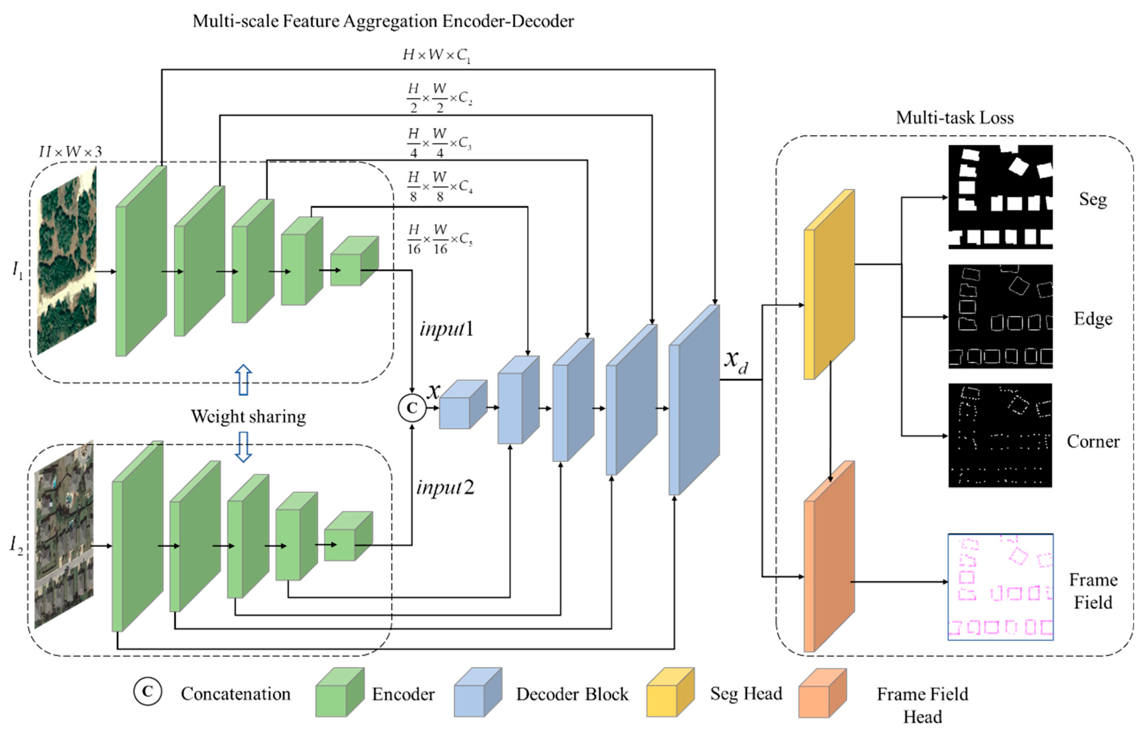
The network first inputs the bi-temporal remote sensing images into a multi-scale feature aggregation encoder–decoder module. Through a multi-layer convolutional structure, it extracts building features at different scales, ensuring that the network perceives both the global structure and local details of the buildings. A cross-attention mechanism is then introduced to enhance the feature correlation between the two temporal images, allowing the network to accurately capture change regions and suppress background noise interference.

Next, the network models the overall building segmentation, edge contours, and corner characteristics using frame fields. The frame fields represent local geometric features through orthogonal vector fields, outputting a four-band frame field result that aids the network in refining the geometric structure of buildings. Simultaneously, the network outputs three segmentation bands: one for overall building segmentation, one for building edge extraction, and one for corner detection. This ensures the network can produce a structured representation of the buildings.

Finally, the tasks are jointly optimized using a multi-task learning strategy, with a loss function that considers both segmentation accuracy and frame field accuracy, ensuring improved performance across all sub-tasks. The network ultimately outputs precise building change detection results, enabling a refined polygonal representation of the changed buildings. The architecture is illustrated in Figure 1.

3.2. Multi-Scale Feature Aggregation Encoder–Decoder Module

The network input consists of remote sensing images captured at two different time points (bi-temporal images), representing the states of buildings before and after changes. To effectively extract the geometric features of building changes from these images, the input is first processed through a multi-scale feature aggregation module.

The encoder architecture is based on ResNet34, excluding the average pooling layer, to extract features across four downsampling stages. For an input size of $256\times 256$, the feature map sizes at each stage are $128\times 128$, $64\times 64$, $32\times 32$, and $16\times 16$, respectively. Through multi-layer convolution operations, features at different scales are extracted, ensuring that the network captures both the global structural information and the local detail of buildings. The advantage of multi-scale feature extraction lies in its ability to adapt to variations in building size, shape, and structure. Whether dealing with large building complexes or smaller structures, this module is capable of extracting the corresponding effective features. This stage of feature extraction provides rich contextual and geometric information for the subsequent building change detection.

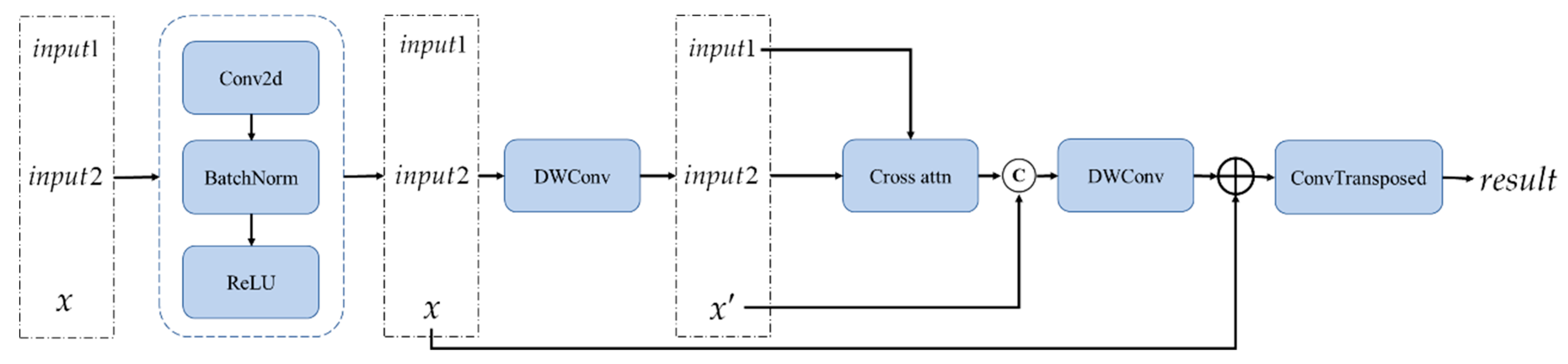
The decoder block includes multiple convolution layers, attention mechanisms, and deconvolution (transposed convolution) operations, which are designed to process and reconstruct the input features. The detailed structure of the network is as follows.

The three input tensors—$input1$, $input$, and $input2$—are concatenated along the channel dimension. The concatenated features are then processed with a $1\times 1$ convolution to reduce the number of channels, followed by batch normalization (BatchNorm) and a ReLU activation function for non-linear transformation. These features are further refined using depthwise separable convolution (DWConv) to extract more detailed information, which is then fed into the cross-attention module.

After the cross-attention mechanism, another depthwise separable convolution is applied to the features. The initial convolution output (denoted as $x$) is added back to the current features $x^{\prime }$ to form a residual connection. A final $1\times 1$ convolution is performed, and the features are upsampled using a transposed convolution (ConvTranspose2d) to generate the final feature map $result$.

The process is formally expressed in Equations (1)–(7).

$$input1,input2,x=\mathrm{Re}\mathrm{LU}(\mathrm{BatchNorm}(\mathrm{Conv}2\mathrm{d}(input1,input2,x)))$$

(1)

$$input1,input2,x^{\prime }=\mathrm{DWConv}(input1,input2,x)$$

(2)

$$attn1,attn2=\mathrm{cross} \mathrm{attn}(input1,input2)$$

(3)

$$x^{\prime }=\mathrm{cat}(attn1,attn2,x^{\prime })$$

(4)

$$x^{\prime }=\mathrm{DWConv}(x^{\prime })$$

(5)

$$x=x+x^{\prime }$$

(6)

$$result=\mathrm{ConvTranspose}2\mathrm{d}(x)$$

(7)

The variable $x$ represents the output $result$ from the previous decoder, while $input1$ and $input2$ are the outputs from the encoder at the corresponding resolution. For the first decoder, $x$ is computed in Equations (8) and (9).

$$x=\mathrm{Re}\mathrm{LU}(\mathrm{BatchNorm}(\mathrm{Conv}2\mathrm{d}(\mathrm{cat}(input1,input2))))$$

(8)

$$x=\mathrm{ConvTranspose}2\mathrm{d}(\mathrm{DWConv}(x\left)\right)$$

(9)

The feature map generated by the last decoder is denoted as $x_d$. A schematic diagram of the decoder process is shown in Figure 2.

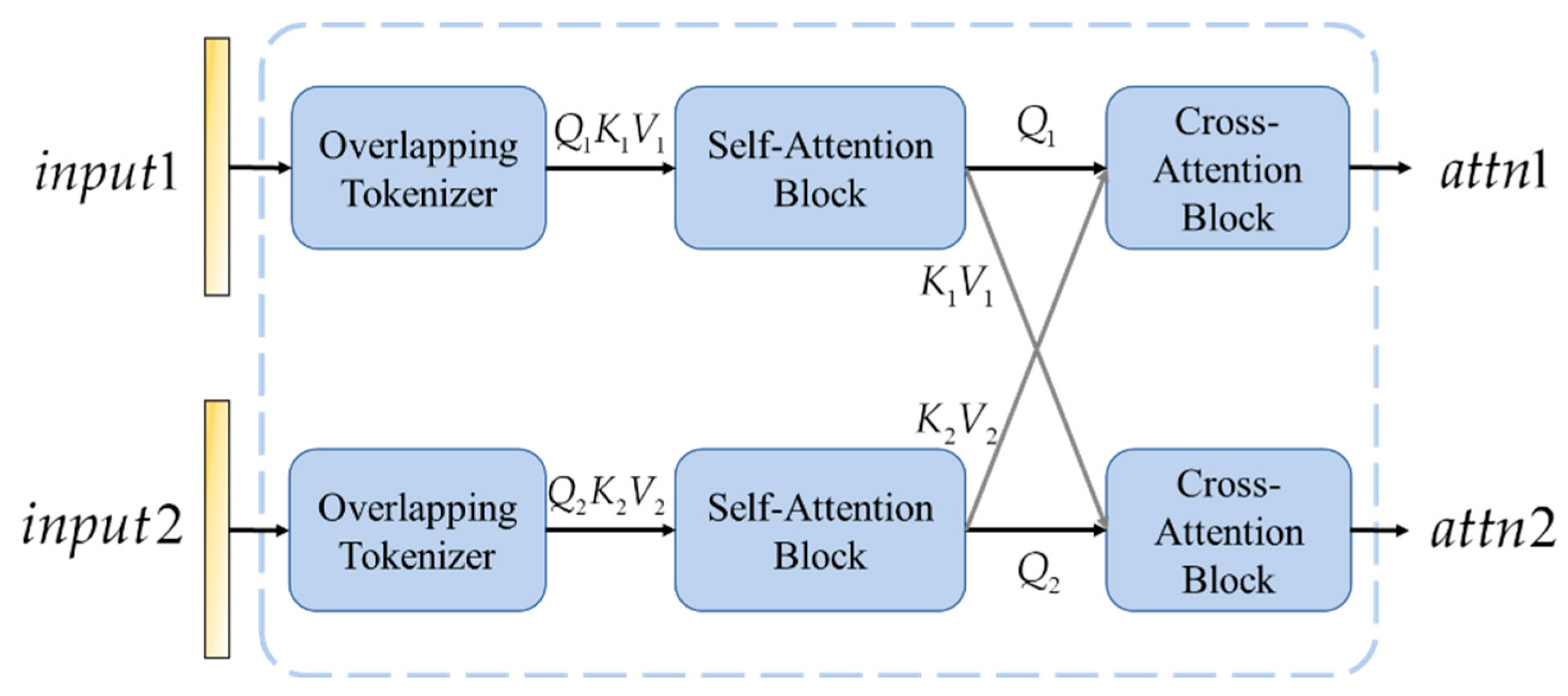
The design of the cross-attention mechanism, used in the process above, is inspired by the feature inconsistencies typically observed in change areas between two time-series images. Specifically, the cross-attention mechanism enhances the correlation between features from both time periods, enabling the network to more accurately pinpoint changes in the buildings. Cross-attention not only adapts the weight distribution across different regions of the images but also effectively suppresses background noise, ensuring that the network focuses on the feature extraction and analysis of changed buildings. By progressively matching and refining the bi-temporal features, this mechanism establishes a solid foundation for building change detection in complex urban environments.

To effectively integrate information from multiple time points, facilitating a more comprehensive understanding of dynamic changes in time-series data, the proposed method employs a cross-attention block composed of a combination of self-attention and cross-attention mechanisms in cascade. Its structure and calculation formula are shown in Equations (10) and (11).

$$SA(X_1)=soft\max ({\displaystyle \frac{Q_1{K}_1^T}{\sqrt{d_k}}})V_1$$

(10)

$$CA(X_1)=soft\max ({\displaystyle \frac{Q_1{K}_2^T}{\sqrt{d_k}}})V_2$$

(11)

The architecture of the cross-attention is shown in Figure 3.

Where $Q$, $K$, and $V$ represent the query, key, and value matrices, respectively, which are derived from the features of the pre-change and post-change images. $d_k$ denotes the dimensionality of the key vectors. Through this attention calculation, the model enhances the feature representation by focusing more on the regions of change when processing images from two different time points, thus improving the accuracy of change detection.

This enhanced attention mechanism allows the model to handle complex urban scenes more effectively by distinguishing actual changes from background noise. Additionally, it contributes to improved generalization by learning correlations between images taken at different times. Cross-attention helps the model generalize across diverse datasets and environmental conditions, thereby enhancing the robustness of change detection. By weighting the features from different time points, the model emphasizes areas with significant changes, which improves the discrimination between changed and unchanged regions. This means that the model can automatically prioritize the most important information based on the observed image content, allowing it to adapt flexibly to varying environmental conditions.

The final feature map $x_d$ is then passed through the multilevel segmentation prediction head and the frame field prediction head, generating multi-head outputs that are further used to calculate the loss.

To comprehensively capture the geometric characteristics of buildings, the multilevel segmentation prediction head is designed to analyze building changes from three levels: point, line, and surface. Accordingly, the outputs include the overall building segmentation, building edges, and building corner points. These results are generated through a multi-output classifier with three output channels, rather than three separate single-channel classifiers. The computation process is shown in Equation (12):

$$outpu{t}_{seg}=\mathrm{Conv}2\mathrm{d}(\mathrm{Re}\mathrm{LU}(\mathrm{BatchNorm}(\mathrm{Conv}2\mathrm{d}(x_d))))$$

(12)

This approach enables a more detailed and structured representation of building changes in complex environments.

3.3. Frame Field

In the task of building change detection, changes in the shape and contour of the buildings are critical factors. Traditional change detection methods often succeed in segmenting the main structures of the buildings but tend to blur at the boundaries, especially at corners and straight edges, resulting in rounded corners or non-linear boundaries. This highlights the need for a more effective approach to consider building characteristics and integrate them into deep neural networks.

Frame fields are a mathematical tool used to describe the directional and structural information of geometric objects on a plane, particularly suited for objects with regular boundaries, such as building contours. A frame field assigns two paired directions at each point to capture the local geometric structure, such as parallel or perpendicular edges. This dual-direction representation is particularly well suited for detecting right angles, boundaries, and corners of buildings. In a frame field, two directions are assigned to each pixel in the image, represented by the complex numbers $u$ and $v$. These directions typically correspond to the primary orientations of building edges, such as parallel walls and perpendicular boundaries.

Following the method proposed by Nicolas Girard [61], to simplify the representation, the frame field is expressed by constructing a fourth-degree complex polynomial that captures the combination of these two directions. The equation for the polynomial is shown in Equation (13).

$$f(x)=(x^2-u^2)(x^2-v^2)=x^4+a_1{x}^2+b$$

(13)

where $x$ is a complex variable representing one of the directional information at a given pixel, while $a,b$ are two sparse polynomials to be learned, denoting the intensity of the decomposed components $u$ and $v$ in the orthogonal field. When $a,b$ are known, the orthogonal directions $u$ and $v$ can be expressed in Equations (14) and (15).

$$u=\sqrt{-{\displaystyle \frac{1}{2}}(a+\sqrt{a^2-4b})}$$

(14)

$$v=\sqrt{-{\displaystyle \frac{1}{2}}(a-\sqrt{a^2-4b})}$$

(15)

This complex form ensures the continuity and invariance of the frame field directions, avoiding inconsistencies caused by changes in sign or directional order. This makes it highly suitable for modeling the characteristics of buildings. We incorporated this frame field representation into the building change detection network.

In the network, the frame field was generated through an additional prediction head that outputted the complex coefficients. These coefficients were not directly used for loss computation but were compared against the geometric structure of building edges for alignment-based loss calculations. For instance, the directional information generated by the frame field was compared with the tangent directions of building edges to compute alignment losses. Furthermore, the output of the frame field was linked to the gradient of the segmentation results, and a coupled loss function ensured the consistency between the segmentation and the frame field output (details of this process are discussed in Section 3.4).

Thus, the primary role of the frame field in the learning process was to provide directional information that complements the segmentation results, particularly at the edges and corners. By integrating this directional alignment into the loss function, the model performance was optimized.

Equation (16) is the calculation process for the frame field prediction head:

$$outpu{t}_{frame}=\mathrm{Conv}2\mathrm{d}(\mathrm{Re}\mathrm{LU}(\mathrm{BatchNorm}(\mathrm{Conv}2\mathrm{d}(\mathrm{cat}(x_d,outpu{t}_{seg})))))$$

(16)

The frame field can accurately capture the geometric characteristics of buildings, particularly in edge regions. By aligning with the tangent directions of building polygons, it ensures more precise boundary extraction. This is especially critical for complex and irregularly shaped buildings, as it effectively reduces edge blur and detection errors. Moreover, at the corners of polygons, the frame field aligns with two tangent directions simultaneously, allowing it to better capture the corner features of buildings.

Compared with traditional vector fields, the frame field is better suited for handling areas with complex building structures. It can generate more regular polygonal representations, especially at corner points. With the integration of the frame field, the model can maintain global geometric consistency when capturing building information, resulting in more natural and coherent building shapes in the change detection outputs. This enhancement not only improves detection accuracy but also ensures that building forms in the output align more closely with real-world geometry.

3.4. Multi-Task Learning Loss

To optimize the network training process, a multi-task learning strategy was adopted, and a loss function was designed to account for both segmentation and frame field accuracy. This multi-task approach allowed simultaneous optimization of segmentation, edge detection, and corner extraction, enhancing the overall building change detection accuracy. The loss function aligned the predicted frame field with the actual building contours and dynamically adjusted task weights based on performance. This design improved the sensitivity to geometric features and reduced false positives and missed detections, ensuring high accuracy in complex scenarios. The details are as follows:

(1) Segmentation Loss $L_{seg}$: The segmentation loss consisted of three parts, building segmentation $L_{building}$, building edge extraction $L_{edge}$, and building corner detection $L_{corner}$, all using cross-entropy loss. This comprehensive approach helped reduce rounded corners and blurred edges. The loss function is defined in Equations (17)–(20).

$$L_{building}=-{\displaystyle \frac{1}{N}}{\displaystyle \sum _{i=1}^N\left[y_{buildingi}\log ({\widehat{y}}_{buildingi})+(1-y_{buildingi})\log (1-{\widehat{y}}_{buildingi})\right]}$$

(17)

$$L_{edge}=-{\displaystyle \frac{1}{N}}{\displaystyle \sum _{i=1}^N\left[y_{edgei}\log ({\widehat{y}}_{edgei})+(1-y_{edgei})\log (1-{\widehat{y}}_{edgei})\right]}$$

(18)

$$L_{corner}=-{\displaystyle \frac{1}{N}}{\displaystyle \sum _{i=1}^N\left[y_{corneri}\log ({\widehat{y}}_{corneri})+(1-y_{corneri})\log (1-{\widehat{y}}_{corneri})\right]}$$

(19)

$$L_{seg}=L_{buinding}+L_{edge}+L_{corner}$$

(20)

where $N$ is the total number of samples, $y_{buildingi}$, $y_{edgei}$, and $y_{corneri}$ are the ground truth label of the i-th sample for building segmentation, edge, and corner, and ${\widehat{y}}_{buildingi}$, ${\widehat{y}}_{edgei}$, and ${\widehat{y}}_{corneri}$ are the corresponding predicted outputs.

(2) Frame Field Loss $L_{frame}$: The frame field loss included three primary components:

Alignment Loss $L_{frame}$: it ensures that the frame field directions align with the tangent directions of the building edges. The direction information generated by the frame field is used to calculate this loss, which optimizes the consistency between the complex coefficients of the frame field and the geometric direction (tangent) of the building contours.

Orthogonal Alignment Loss $L_{orthogonal}$: it ensures that the frame field does not degenerate into a single-direction field. It encourages the orthogonal direction of the frame field to align with the building edge’s normal direction.

Smoothing Loss $L_{smooth}$: the loss ensures the frame field directions are spatially smooth and continuous. It constrains the directional changes in the frame field between neighboring pixels, leading to smoother and more natural frame field outputs. The formula for the frame field loss is shown in Equations (21)–(24).

$$L_{align}={\displaystyle \frac{1}{HW}}{{\displaystyle \sum _{x\in I}{y}_{edge}(x)\left|f(e^{i{\theta }_{\tau }};\widehat{a}(x),\widehat{b}(x))\right|}}^2$$

(21)

$$L_{orthogonal}={\displaystyle \frac{1}{HW}}{{\displaystyle \sum _{x\in I}{y}_{edge}(x)\left|f(e^{i{\theta }_{\tau \perp }};\widehat{a}(x),\widehat{b}(x))\right|}}^2$$

(22)

$$L_{smooth}={\displaystyle \frac{1}{HW}}{\displaystyle \sum _{x\in I}({‖\nabla \widehat{a}(x)‖}^2+{‖\nabla \widehat{b}(x)‖}^2)}$$

(23)

$$L_{frame}=L_{align}+L_{orthogonal}+L_{smooth}$$

(24)

where $H$ and $W$ represent the image height and width, and $x\in I$ denotes a pixel in the image. $y_{edge}(x)$ represents the probability map of the building edges, where edge pixels are marked as 1 and others as 0. ${\theta }_{\tau }$ represents the tangent direction at the building edge, while ${\theta }_{\tau \perp }$ denotes the normal direction perpendicular to the tangent. The polynomial $f(e^{i{\theta }_{\tau }};\widehat{a}(x),\widehat{b}(x))$ is derived from the frame field output, with its roots aligned with the tangent direction. $\nabla \widehat{a}(x),\nabla \widehat{b}(x)$ represents the gradient of the complex coefficients $a,b$ at pixel $x$, reflecting the rate of change in the frame field across the image. The ground truth for the frame field is obtained by referencing the method outlined in [61]. The final loss is the sum of the segmentation loss and the frame field loss, as shown in Equation (25), with a weight coefficient $\alpha$, empirically set to 0.5, to be further discussed in subsequent sections.

$$L_{final}=L_{seg}+\alpha \cdot L_{frame}$$

(25)

This multi-task learning loss function ensures that the network can accurately capture and represent the geometric features of buildings at multiple levels. This manuscript method models and decomposes the geometric properties of buildings at various levels.. First, the segmentation head extracts the building shape, capturing its basic structure. Then, it refines the building boundaries, ensuring edge precision. Finally, it identifies corner points, capturing key geometric features to enhance the representation of complex polygonal structures. In addition, the frame field head provides multi-band frame field outputs, delivering higher-level geometric information from global to local scales. This ensures accurate modeling of building geometry across different scales and levels. The fusion of these multilevel geometric details significantly improves both the performance and the accuracy of detail handling in building change detection tasks.

4. Results

This section presents the datasets, evaluation metrics, comparison with the state-of-the-art methods, discussion on parameter count and computational complexity, ablation study, and analysis of loss weight coefficients.

4.1. Datasets

For the building change detection task, two commonly used public datasets were selected: LEVIR and WHU.

The LEVIR dataset was collected from Google Earth, and the data in it were all RGB images. The LEVIR consisted of image patches of size $1024\times 1024$ pixels with a resolution of 0.5m. It contained 637 pairs of high-resolution remote sensing images, each representing the same area at different times (usually years apart). The dataset was used to detect building changes, such as the addition, demolition, or modification of structures. Since processing $1024\times 1024$ images consumed considerable computational resources, we followed the common practice adopted in other studies by splitting them into 10,192 pairs of $256\times 256$ image patches. The dataset was divided into a training set, validation set, and test set in a ratio of 7:1:2, with 7120, 1024, and 2048 pairs, respectively. Each image pair was accompanied by a binary change mask (ground truth mask), where white (1) indicated areas of change, and black (0) indicated unchanged areas. These masks were used to train the model to identify building changes within the images.

The WHU dataset was collected from cities around the world and various remote sensing resources, including QuickBird, Worldview series, IKONOS, and ZY-3. The WHU dataset captured building changes between 2012 and 2016. The original image, measuring $15534\times 32507$ pixels, was divided into multiple $256\times 256$ patches with a resolution of 0.2 m. A total of 7616 image pairs were selected, and split into 6096 pairs for training, 760 pairs for validation and 760 pairs for testing. This dataset included building changes in Christchurch, New Zealand.

4.2. Evaluation Metrics

To objectively evaluate the performance of the proposed BuildingCDNet, we selected several common change detection metrics as evaluation standards: precision (P), recall (R), intersection over union (IoU), F1-score (F1), and overall accuracy (OA). These metrics provided a comprehensive assessment of the accuracy of the change detection. Following other studies, each metric here represented the evaluation results for the change class. The specific calculation formulas are shown in Equations (26)–(30).

$$Precision=TP/(TP+FP)$$

(26)

$$Recall=TP/(TP+FN)$$

(27)

$$IoU=TP/(TP+FN+FP)$$

(28)

$$F1=2/(Precisio{n}^{-1}+Recal{l}^{-1})$$

(29)

$$OA=(TP+TN)/(TP+TN+FP+FN)$$

(30)

where $TP$, $TN$, $FP$ and $FN$ represent true positives, true negatives, false positives, and false negatives, respectively.

All experiments were conducted in a Windows environment using an NVIDIA RTX 4090 GPU, Python 3.8, and PyTorch 2.4 for training and testing. During training, AdamW was used as the optimizer, with a batch size of 16 and a learning rate set to 0.001.

4.3. Comparison with the State-of-the-Art Methods

The building change detection experiments were conducted on the LEVIR and WHU datasets under the conditions mentioned above. To evaluate the advantages and applicability of the proposed method, the following state-of-the-art comparative methods were selected:

FC-EF [50]: This method is an early-stage single-path network based on U-Net, where two images are concatenated as one input and fed into a fully convolutional network for feature extraction.

FC-Si-diff [50]: This method uses a Siamese network structure to extract features separately from the input images through a dual-path encoding process. In the decoding step, the absolute difference in the two connected encoding streams is concatenated to detect differences between the two images.

STANet [51]: A change detection method that utilizes a self-attention mechanism to model spatiotemporal change relationships. It introduces a self-attention module to compute attention weights between pixels at different times and scales, generating more discriminative features.

BIT [56]: This method was among the first to incorporate a transformer structure into a deep feature difference change detection framework. It uses CNNs to extract high-dimensional features and refines them with a transformer decoder to model spatiotemporal context, achieving superior results compared with fully convolutional networks.

Changeformer [62]: A Siamese network method that uses a hierarchical transformer encoder and MLP decoder, combined with a multi-scale difference calculation module to capture change features. It is a typical pure transformer-based approach.

ICIFNet [63]: A network that combines CNNs and transformer architectures. It incorporates feature cross-fusion at the same scale and cross-scale feature fusion modules, using mask-based aggregation and spatial alignment (SA) methods to achieve better results.

VcT [64]: This method employs a graph neural network (GNN) to model structured information and uses a clustering algorithm to select the Top-K reliable tokens. These tokens are then enhanced through a self/cross-attention (CA) mechanism and deeply interact with original features using the anchor-primary attention (APA) learning module. Finally, a prediction head is introduced to improve change map prediction accuracy.

AERNet [60]: This method integrates enhanced coordinate attention (ECA)-guided attention decoding blocks (ADBs) to capture channel and positional correlations between features. It adopts an edge refinement module (ERM) to improve the network’s perception and refinement of change region edges. Additionally, it designs an adaptive weighted binary cross-entropy (SWBCE) loss function to handle class imbalance issues.

MambaBCD [35]: MambaBCD is a framework within the ChangeMamba method specifically designed for binary change detection in remote sensing images. It uses the Mamba architecture to capture spatiotemporal features, allowing for efficient modeling of both spatial and temporal relationships in multi-temporal data. Through sequential and cross-spatial mechanisms, MambaBCD effectively distinguishes changed and unchanged areas, achieving high accuracy in binary change detection tasks.

The parameters of all comparative methods were kept unchanged, as specified in their respective original papers. The quantitative results of the different methods are shown in

Table 1. Quantitative results of different methods (%): best, 2nd-best, 3rd-best.

Method	LEVIR					WHU
	P	R	IoU	F1	OA	P	R	IoU	F1	OA
FC-EF	86.16	81.12	71.77	83.56	98.27	81.05	74.82	63.68	77.81	97.91
FC-Si-diff	89.36	83.24	75.73	86.19	98.65	84.29	77.77	67.92	80.90	98.20
STANet	85.62	90.74	78.74	88.11	98.34	83.06	87.79	74.46	85.36	98.66
BIT	90.35	88.34	80.72	89.33	98.84	89.13	82.81	75.22	85.86	98.67
Changeformer	91.06	89.11	81.94	90.07	98.94	88.68	85.77	77.30	87.20	98.77
ICIFNet	91.23	88.87	81.79	89.98	98.81	91.64	85.28	79.13	88.35	98.90
VcT	92.28	88.53	82.43	90.37	99.10	91.35	88.49	81.65	89.90	99.12
MambaBCD	91.38	90.25	83.17	90.81	99.12	92.12	88.74	82.48	90.40	99.08
AERNet	91.05	90.28	82.92	90.66	99.12	92.86	88.52	82.88	90.64	99.03
BuildingCDNet	92.08	90.89	84.30	91.48	99.25	92.25	90.49	84.10	91.36	99.16

.

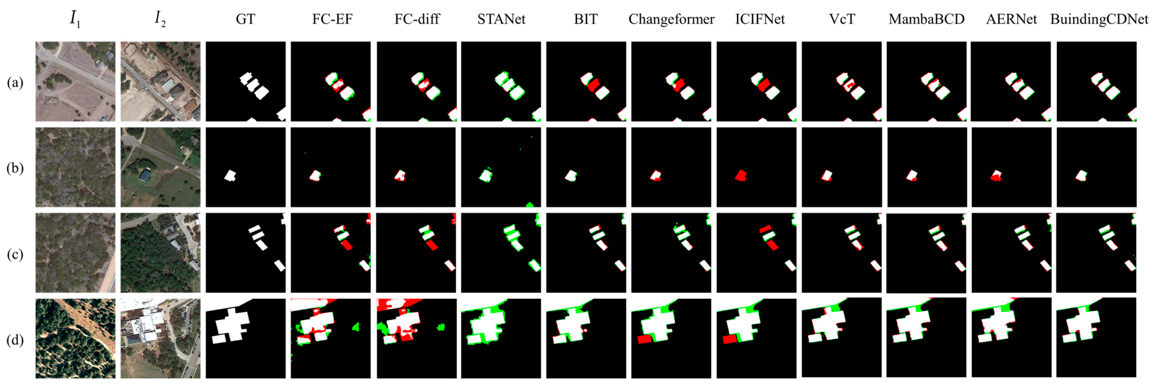
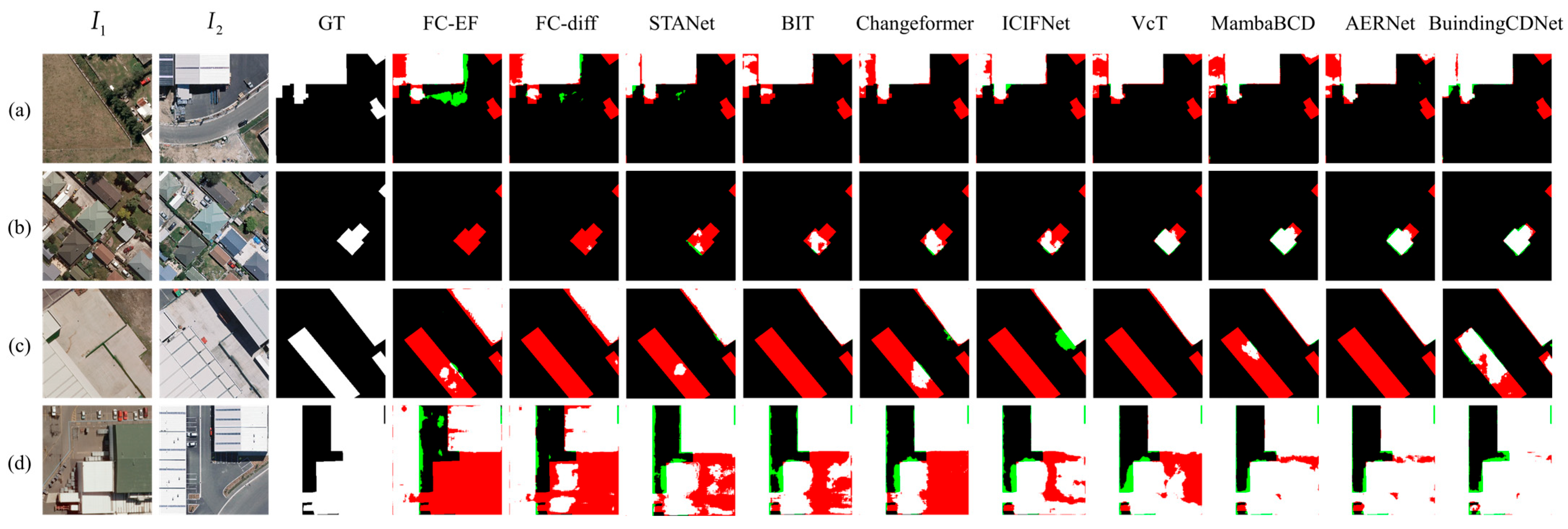
The quantitative results and the visualization results are shown in Figure 4 and Figure 5, where white represents $TP$, black represents $TN$, green represents $FP$, and red represents $FN$.

The performance of each method is analyzed in detail.

Experimental results on the LEVIR dataset demonstrated the effectiveness of various models in change detection tasks. A comparison reveals that BuildingCDNet consistently outperformed the other models across multiple metrics. FC-EF is a relatively basic approach, with lower performance across all metrics. Although its OA reached 98.27%, the F1 score remained relatively low. FC-Si-diff improved upon FC-EF, yielding a higher precision (89.36%); however, its recall (83.24%) remained comparatively low. STANet exhibited strong recall capability, achieving a recall of 90.74%. However, its precision was lower, as indicated by numerous false positives in the green areas of the results. BIT achieved a better balance between precision and recall, with an F1 score of 89.33%. Changeformer further enhanced BIT’s performance, with an IoU of 81.94% and an F1 score of 90.01%. ICIFNet improved precision but had slightly lower recall than some other methods, leading to more missed detections (in red) in the visual results. VcT exceled in precision, achieving the highest precision score of 92.28% among all the methods. MambaBCD effectively captured changes in high-resolution images, striking a good balance between precision (91.38%) and recall (90.25%). Also, the method had competitive IoU and F1 scores. AERNet demonstrated a strong overall performance with an IoU of 82.92% and an F1 score of 90.66%. BuildingCDNet outperformed all the other methods in nearly every metric, except for precision. The visualization results also indicate that BuildingCDNet produced clearer building outlines with fewer false positives and false negatives. Notably, in Figure 4a, other methods failed to fully capture the central building changes, whereas BuildingCDNet delivered more accurate results.

On the WHU dataset, the simpler architectures such as FC-EF and FC-Si-diff showed relatively low performance across all metrics, with numerous false positives and false negatives. The detected building outlines appeared disorganized. STANet achieved notable improvements in F1 and IoU compared with the FC-based methods, but its gains in precision were less significant. The transformer-based methods, BIT and Changeformer, showed substantial improvements in precision, with Changeformer achieving superior results in Figure 5c compared with all the methods except BuildingCDNet. ICIFNet reached a precision of 91.64%, with fewer missed detections and better overall results in Figure 5d. VcT, using a coarse-to-fine transformer architecture combined with a vision-guided attention mechanism, demonstrated excellent performance in both IoU and F1, while also maintaining high precision. MambaBCD maintained a high precision (92.12%), although it was slightly lower than some other methods in terms of recall (88.74%). AERNet, which integrates a residual network with enhanced attention mechanisms, achieved a good balance between precision and recall, delivering strong results. The proposed BuildingCDNet achieved the highest performance across almost all metrics on the WHU dataset. As seen in Figure 5a–d, BuildingCDNet produced the best results, effectively capturing detailed changes and significantly reducing both false positives and missed detections. This makes it particularly well suited for high-precision and high-sensitivity change detection tasks. Overall, the model not only accurately identified change regions but also precisely located these areas, minimizing errors in detection.

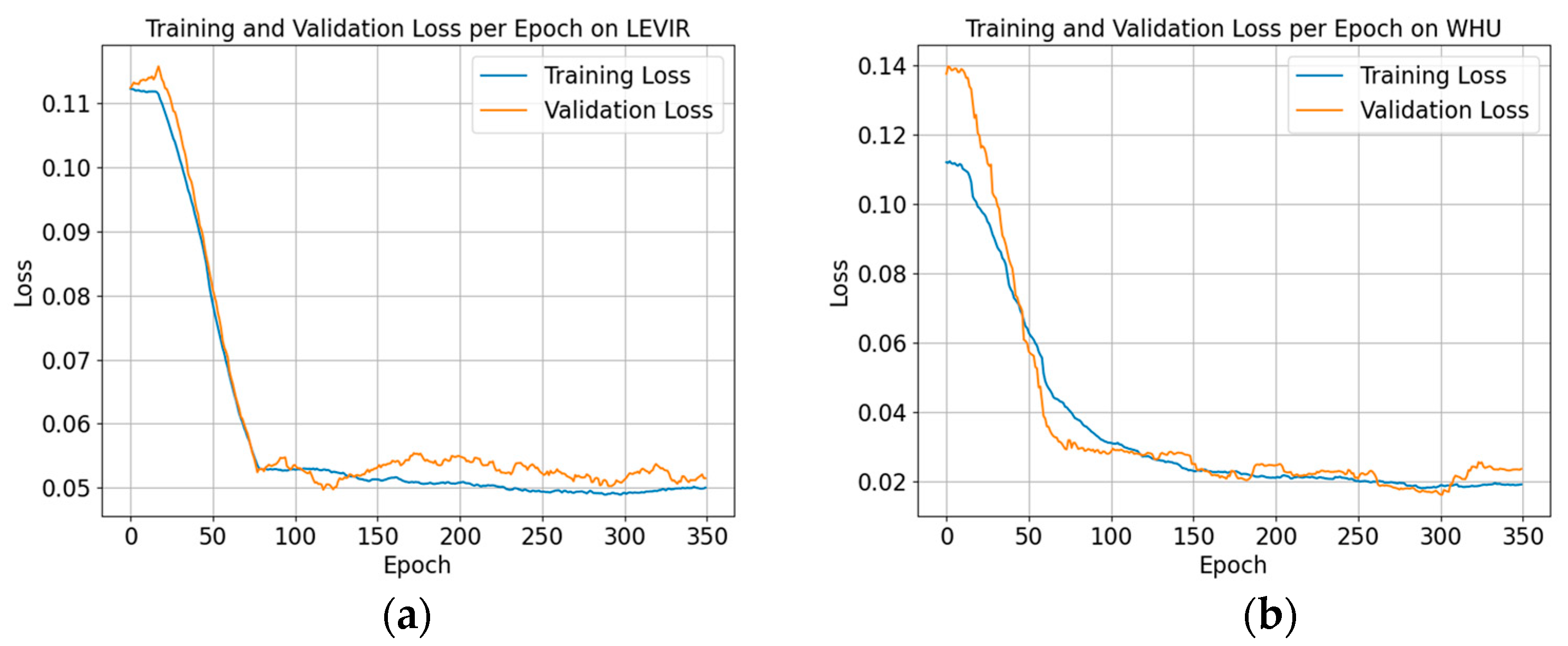
Figure 6 is the training–validation loss per epoch of BuildingCDNet on different datasets.

On the LEVIR dataset, within the first 50 epochs, both training and validation losses dropped rapidly, indicating that the model can quickly learn useful features from this dataset. After around 50 epochs, the loss curves gradually stabilize, suggesting that the model had reached a good level of convergence. The training and validation losses almost overlap, indicating that the model did not exhibit significant overfitting on this dataset, which suggests a good generalization ability on the LEVIR. In the stabilization phase, the validation loss shows minimal fluctuations, which is normal and expected.

On the WHU dataset, the model’s convergence was somewhat slower, and the validation loss decreased more gradually but eventually stabilized. After approximately 50 epochs, the loss curves begin to stabilize. On the WHU dataset, the training loss consistently remained lower than the validation loss, especially in the stabilization phase. This indicates that the model performs better on the training data, with a certain degree of overfitting on the validation data. During the stabilization phase, the validation loss on the WHU dataset shows more noticeable fluctuations, which could be due to more complex characteristics or uneven sample distribution in this dataset.

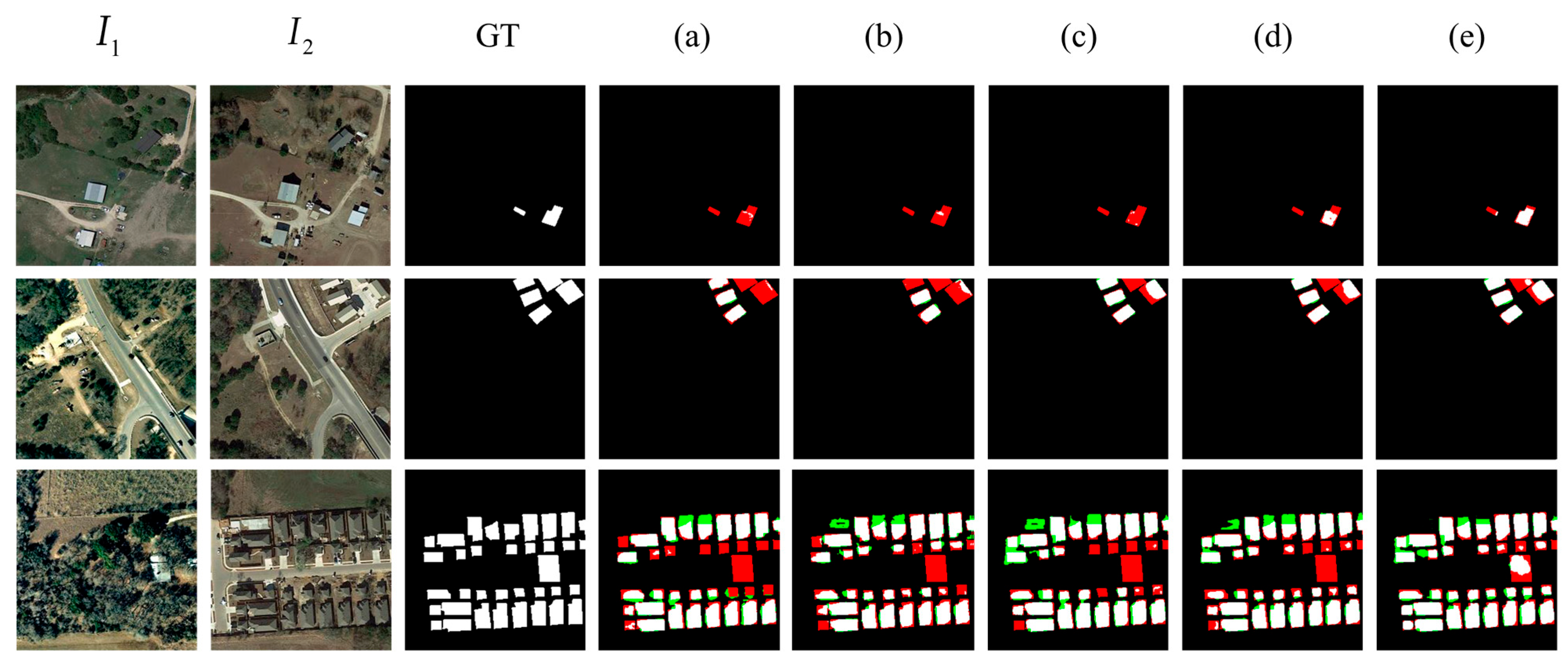
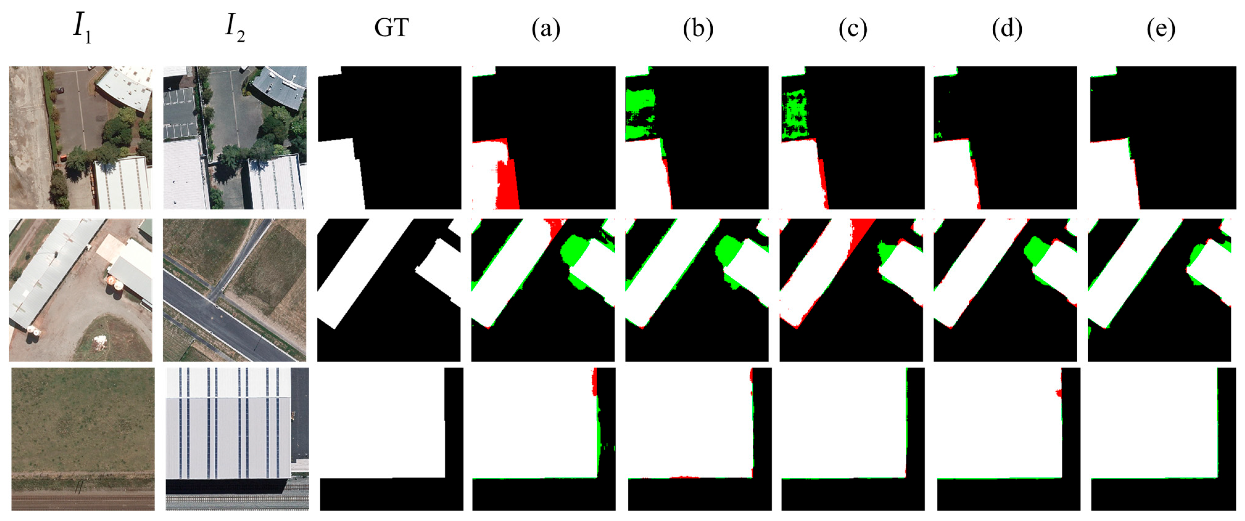
4.4. Ablation Study

To validate the functionality of each component, an ablation study was conducted. The baseline model (denoted as a) utilized only ResNet34 as the encoder, retaining the multi-scale downsampling components. The decoder directly concatenated outputs from different levels without incorporating attention modules, and a single segmentation prediction head was employed. The following experiments analyze and discuss the impact of adding different components: a multi-scale feature aggregation decoder module (denoted as b), cross-attention (denoted as c), multilevel segmentation prediction head (denoted as d), and frame field prediction head (denoted as e).

For each experiment, the loss settings were determined based on the choice of prediction heads. The results are shown in

Table 2. Quantitative results of ablation study on LEVIR dataset (%).

Baseline	MSFADM	CA	MLSPH	FFPH	P	R	IoU	F1	OA
✓					90.83	88.68	81.39	89.74	98.86
✓	✓				91.55	89.36	82.55	90.44	99.04
✓	✓	✓			91.80	89.76	83.10	90.77	99.12
✓	✓	✓	✓		92.70	89.48	83.59	91.06	99.18
✓	✓	✓	✓	✓	92.08	90.89	84.30	91.48	99.25

and

Table 3. Quantitative results of ablation study on WHU dataset (%).

Baseline	MSFADM	CA	MLSPH	FFPH	P	R	IoU	F1	OA
✓					91.05	88.73	81.61	89.88	98.81
✓	✓				91.61	89.20	82.46	90.39	99.04
✓	✓	✓			92.65	88.67	82.84	90.64	99.10
✓	✓	✓	✓		91.51	90.25	83.28	90.88	99.12
✓	✓	✓	✓	✓	92.25	90.49	84.10	91.36	99.16

, as well as in Figure 7 and Figure 8.

The addition of the multi-scale feature aggregation decoder module (MSFADM) significantly improved both precision and recall, indicating enhanced capability in identifying changes and an overall improvement in IoU. This suggests that the model not only detects more changes but also achieves higher segmentation accuracy. As seen in the figures, there was a noticeable reduction in false positives, demonstrating that MSFADM plays a key role in enhancing model performance by effectively combining multi-scale features. However, it may also introduce some false alarms.

The introduction of cross-attention (CA) helped achieve a better balance between precision and recall, improving the overall detection performance. After incorporating CA, the model showed better recall and IoU, enhancing its ability to capture subtle changes. The boundaries of the detected change areas became smoother, and CA enabled more precise localization of change areas by integrating interactions between different inputs.

The multilevel segmentation prediction head (MLSPH) was designed to leverage features from multiple levels, improving the model’s ability to detect objects of varying sizes and complexities. With the inclusion of MLSPH, the model’s performance was further enhanced, particularly in reducing false positives. Notably, in large-scale change areas within the WHU dataset, the model effectively mitigated missed detections. This shows that multilevel feature prediction can significantly improve segmentation accuracy.

The frame field prediction head (FFPH) focused on capturing the geometric characteristics of the buildings, providing more structured segmentation information. The inclusion of this module enhanced the model’s performance in detecting building-related changes, particularly in complex scenes. All key metrics showed improvement, with better accuracy in detecting building outlines and reduced false positives and missed detections. Notably, the model can better differentiate real changes in building corners.

In summary, the progressive addition of MSFADM, CA, MLSPH, and FFPH not only enhances the overall performance of the model but also significantly improves the recognition of complex changes and the accurate segmentation of building structures. The best results were achieved when all modules were integrated, highlighting their essential role in deep learning-based change detection tasks. These findings provide valuable insights for future research and applications in the field.

5. Discussion

5.1. Computation Costs

The following section provides an analysis of the parameter count and computational complexity of each comparison method, along with the proposed method, as shown in

Table 4. Computation costs of different methods.

Method	Params (Mb)	FLOPs (Gbps)	Inference Time (ms)
FC-EF	1.35	3.58	0.26
FC-Si-diff	1.35	4.74	0.35
STANet	16.89	6.58	1.02
BIT	3.50	10.63	0.66
Changeformer	41.03	202.79	5.11
ICIFNet	23.84	24.51	1.79
VcT	3.57	10.64	0.92
MambaBCD	84.70	179.32	4.22
AERNet	25.36	12.82	1.68
BuildingCDNet	24.04	12.79	1.51

.

From the comparison of parameter count (Params) and computational complexity (FLOPs) in Table 4, it can be observed that BuildingCDNet maintains excellent performance while keeping its computational overhead relatively moderate. The methods FC-EF and FC-Si-diff have the lowest parameter counts, both at 1.35 Mb, indicating that their computational cost is extremely low. However, despite the small computation load, their performance in practical applications is suboptimal. STANet exhibits higher computational costs compared with the FC series models, but it shows significant improvements, particularly in recall. BIT has a much higher computational load than both STANet and the FC models, achieving a better balance between precision and recall. Although Changeformer and MambaBCD delivers outstanding performance in precision, recall, and IoU, the high computational cost may pose challenges regarding resource consumption. ICIFNet strikes a balance between performance and computational load, with a parameter count of 23.84 Mb and FLOPs of 24.51 Gbps. VcT has computational costs comparable to BIT and achieves slightly better performance. Its high precision demonstrates that it achieves impressive detection results with a reasonable computational load. AERNet maintains moderate computational costs while delivering strong precision and recall, showcasing its ability to achieve solid performance with relatively low resource consumption. BuildingCDNet has a parameter count of 24.04 Mb and FLOPs of 12.79 Gbps. Among all high-performance models, its computational overhead is relatively moderate. Although BuildingCDNet’s parameter count and FLOPs exceed those of simpler models such as STANet and BIT, it significantly reduces the computational cost compared with more complex models like Changeformer. Despite this reduction in complexity, BuildingCDNet achieves the highest or near-highest values across all evaluation metrics.

For inference time (the time it takes for a model to make one prediction on a set of input data), there are significant differences among the models: FC-EF and FC-Si-diff have the shortest inference time but at the same time have poorer accuracy; Changeformer and MambaBCD are complex models and have a longer inference time; ICIFNet, VcT, and AERNet have relatively faster inference speeds and fair accuracy. ICIFNet, VcT, and AERNet have relatively fast inference speeds and fair accuracy. BuildingCDNet achieves a better balance between the inference time (1.51 ms), number of parameters and FLOPs, and takes into account the accuracy and efficiency.

Thus, BuildingCDNet strikes an ideal balance between performance and computational efficiency, demonstrating its ability to achieve optimal performance with reasonable computational resources.

5.2. Parameter Analysis

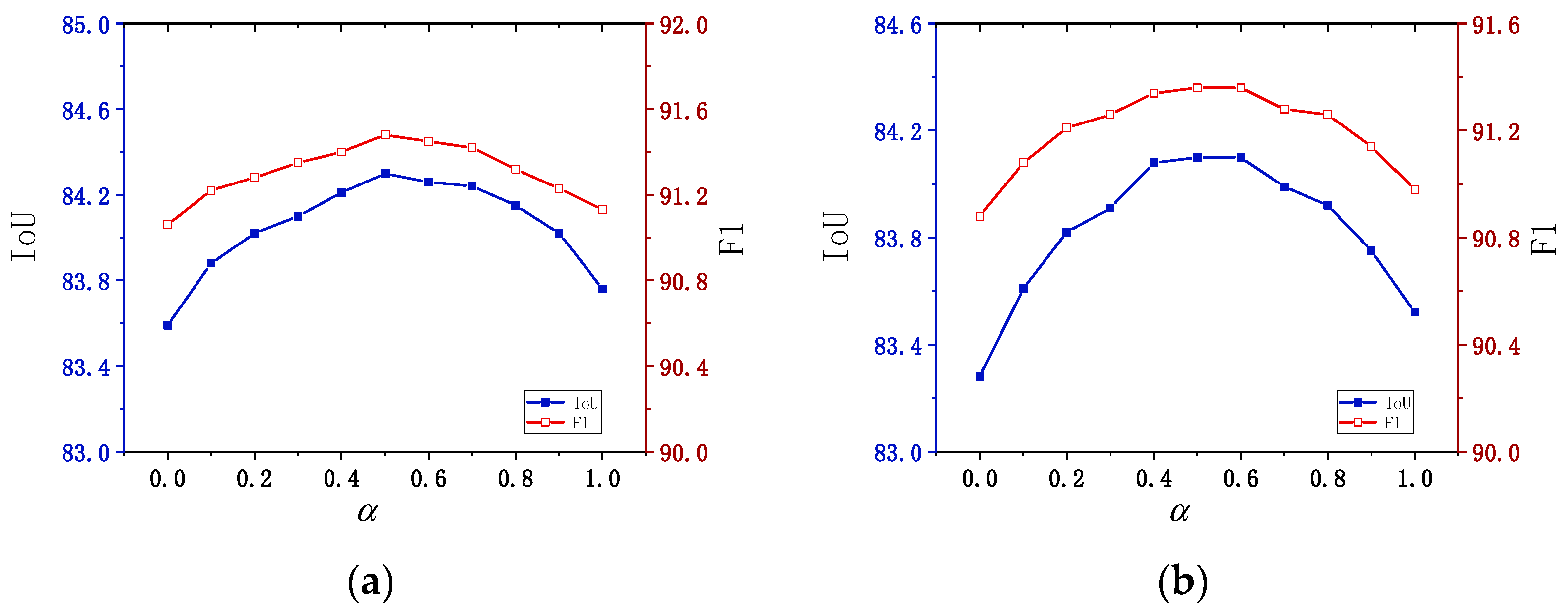
This section analyzes and discusses the impact of the weight parameter $\alpha$ in the multi-task loss function. The value of $\alpha$ was varied from 0 to 1, with increments of 0.1, and the model performance was evaluated based on two comprehensive metrics: IoU and F1 score.

Figure 9 above illustrates how the parameter $\alpha$ (the balancing coefficient between segmentation loss and frame field loss) affects the model’s performance, tested on both the LEVIR and WHU datasets. Below is a detailed analysis of the experimental results.

LEVIR dataset analysis: As $\alpha$ increases from 0 to 0.5, the IoU score gradually rises, peaking at 84.30 when $\alpha =0.5$. After $\alpha$ surpasses 0.5, the IoU score slightly decreases. The optimal $\alpha$ value, around 0.5, achieved the best IoU (84.30), indicating that this value strikes the best balance between segmentation loss and frame field loss. A similar trend is observed with the F1 score, which increases initially as $\alpha$ rises, reaching a maximum of 91.48 at $\alpha =0.5$. This suggests that $\alpha =0.5$ represents an ideal balance point, resulting in the optimal trade-off between precision and recall, and thus the best overall model performance.

WHU dataset analysis: For the WHU dataset, IoU increases steadily as $\alpha$ rises from 0 to 0.5, reaching a maximum of 84.10. When $\alpha$ exceeds 0.6, the IoU begins to decrease, mirroring the trend observed on the LEVIR dataset. This indicates that placing too much emphasis on the frame field loss negatively impacts segmentation performance. The best $\alpha$ value was 0.5 and 0.6, which also produced the highest IoU on the WHU dataset. The F1 score peaked at 91.36 when $\alpha$ reached 0.5, suggesting that, for the WHU dataset, a slightly higher frame field weight may further balance segmentation loss. However, similar to IoU, the F1 score began to decline when $\alpha$ becomes too large.

Across both datasets, the experimental results indicate that an $\alpha$ value between 0.5 and 0.6 is optimal for balancing segmentation loss and frame field loss. This range provides an ideal trade-off that maintains high IoU while enhancing the F1 score. As $\alpha$ increased beyond 0.6, the model’s performance (in terms of both IoU and F1) declined, suggesting that while the frame field loss is important, assigning it too much weight can reduce segmentation accuracy and degrade overall performance. Therefore, it is recommended to set $\alpha =0.5$ for final model tuning, ensuring a well-balanced trade-off between segmentation and frame field losses.

6. Conclusions

This paper proposes a building change detection network optimized through multilevel geometric representation using frame fields, aimed at addressing the limitations of existing methods in complex urban environments, such as irregular boundaries and insufficient segmentation accuracy. The network integrates frame fields for comprehensive geometric modeling of building segmentation, edge contours, and corner points, along with a multi-scale feature aggregation encoder–decoder module and cross-attention mechanism. This design aims to accurately capture the geometric characteristics of buildings and achieve high-precision change detection.

Experimental results demonstrate significant performance improvements on multiple high-resolution remote sensing datasets, particularly in scenarios involving complex building structures and blurred boundaries, where both segmentation accuracy and contour alignment are notably optimized. Compared with existing change detection methods, the proposed model excels not only in global segmentation but also in generating more regular and precise polygonal representations of buildings by thoroughly modeling edges and corners. Furthermore, the design of multi-task learning and an innovative loss function enhances the network’s ability to discriminate building structural information, effectively reducing false positives and missed detections.

Overall, the multilevel geometric optimization approach based on frame fields offers an efficient and precise solution for building change detection. It also provides a valuable reference for future building detection and analysis tasks. Future research could extend this method to other complex object change detection tasks and explore deeper geometric feature modeling and optimization strategies to further improve the model’s robustness and generalization.