Abstract
The BeiDou Navigation Satellite System (BDS-3) has officially provided services worldwide since July 2020. BDS-3 has added new signals for B1C, B2a and B2b based on old BDS-2 B1I and B3I signals, which brings opportunities for achieving high-precision time transfer. In this research, the BDS-3/BDS-2 combined penta-frequency common-view (CV) single-differenced (SD) precise time transfer model is established with B1I, B3I, B2I, B1C, B2a and B2b signals, including dual-, triple-, quad- and penta-frequency (abbreviated as DF, TF, QF and PF) ionosphere-free (IF) combination CV SD models. Taking four long baseline time links (from 637.6 km to 1331.6 km) as examples, the accuracy and frequency stability of the BDS-3/BDS-2 combined DF, TF, QF and PF SD time transfer models were evaluated. The experimental results show that the frequency stability of the TF, QF and PF SD models were improved by 2.5%, 5.3% and 8.5%, on average, over the DF SD model. Compared with the traditional DF (B1I/B3I IF combination) SD model, the standard deviation (STD) of the multi-frequency SD model was reduced by 5.9%, on average, and the frequency stability was improved by 4.0% on average, which had the most apparent effect on the improvement of short-term frequency stability. Specifically, the DF1 (B1C and B2a DF IF combination), TF1 (B1C, B2a and B2b TF IF combination), QF1 (B1C, B1I, B2a and B2b QF IF combination) and PF4 (B1C, B1I, B2a, B2b and B3I PF IF combination) SD models had better performance in timing, and the PF4 SD model had the best performance. Considering that the PF4 (one PF signal IF combination) SD model does not require an estimated inter-frequency bias and that its noise factor is minor compared with the PF1 (four DF signal IF combination), PF2 (three TF signal IF combination) and PF3 (two QF signal IF combination) SD models, we recommend the PF4 SD model for multi-frequency time transfer and the use of the PF2, PF2 or PF3 SD model to supplement the PF4 SD model in cases of penta-frequency observation loss.
1. Introduction
As a constellation transmitting penta-frequency signals, the BeiDou Navigation Satellite System (BDS-3) has provided positioning, navigation and timing (PNT) services since July 2020. It is compatible with old BDS-2 B1I and B3I signals and adds B1C, B2a and B2b new signals [1,2,3,4] (the frequencies of BDS-3 B2b and BDS-2 B2I are the same, but the modulation methods are different). The penta-frequency signals of BDS have created conditions for high-precision time transfer and provided opportunities for the maintenance and implementation of spatiotemporal benchmarks in the era of precision measurement.
Regarding the potential advantages of multi-frequency signals in further observation, ionosphere-free (IF) combinations, fixing ambiguity and cycle slip detection, scholars have conducted research on the model of BDS multi-frequency signals, tested and evaluated its performance in various fields and assessed the advanced performance of multi-frequency signals [5,6,7,8,9]. IGS analysis centers (such as Wuhan University (WHU)) have been able to provide code and phase bias products for BDS multi-frequency signals [10], as well as providing conditions for the application of BDS-3 penta-frequency (PF) signals. Scientists have conducted extensive experiments on the reliability of BDS-3 multi-frequency precise point positioning (PPP) in response to the advantages of multi-frequency-signal minimum noise and quickly fixing undifferenced ambiguity [11,12,13,14,15]. Since then, the application of multi-frequency signals has gradually expanded to the time-frequency field, and a large number of technologies in multi-frequency precision positioning have also been continued in time transfer [16,17,18]. Now, the Global Navigation Satellite System (GNSS) PPP time transfer accuracy and frequency stability can reach sub-ns and sub-10−16@10 day [19,20,21]. At the same time, extensive research has evaluated the models and performance of BDS-3 triple-frequency (TF), quad-frequency (QF), and PF undifferenced (UD) IF combination PPP time transfer, and the accuracy and frequency stability advantages of multi-frequency signals over traditional dual-frequency (DF) signals in UD PPP timing have been demonstrated, especially in short-term frequency stability [22,23,24,25,26,27,28,29,30].
Furthermore, considering that the carrier phase single-differenced (SD) (also known as carrier phase common-view (CP-CV)) model [31] can further weaken the satellite-related errors compared with the UD PPP model, the SD model with BDS multi-frequency observations may have more advantages than the PPP model in time transfer. However, perhaps due to the influence of SD usage distance and the difficulty of processing long baselines, there is relatively little research on SD time transfer, and all the relevant studies focus on GPS and short baselines [32,33,34,35,36]. These studies have demonstrated that SD has certain accuracy advantages over UD PPP in timing, especially in the case of a short baseline. Hence, the BDS multi-frequency long baseline SD time transfer model is still worth studying, exploring and evaluating. The current high-precision multi-frequency and multi-GNSS satellite products, the refinement of error models and the large number of common-view satellites make the precise solution of a long baseline possible, guaranteeing the realization of precise SD time transfer.
Previous studies have focused more on BDS UD PPP or GPS SD time transfer, and there has been no research on establishing the BDS-2/BDS-3 combined multi-frequency SD timing model. Moreover, with the rapid development of BDS multi-frequency signals, the previous SD time transfer research has had difficulty in adapting to the current environment. BDS multi-frequency signals will bring more IF combination space, smaller noise coefficients, more observations, and advantages to SD models, so the BDS multi-frequency SD time transmission will have more significant potential. This research proposes BDS-3/BDS-2 combined CV SD time transfer models with BDS-2 B1I, B2I and B3I and BDS-3 B1I, B2b, B3I, B1C and B2a multi-observations, and a comprehensive analysis and an evaluation of the performance of BDS multi-frequency SD time transfer were conducted.
The structure of this research includes the following: Firstly, the function model and stochastic model of the PF CV SD time transfer of BDS-2/BDS-3 combination are studied, and the coefficients of the DF to PF IF combination are given. Secondly, four-time transfer links with high-precision atomic clocks are selected to compare and evaluate the performance of the DF to PF SD time transfer models. Finally, the research work is discussed, and the conclusion is given.
2. Methodology
2.1. DF IF Combination SD Time Transfer Function Model
Take the B1I and B3I signals as examples, and select the BDS-3 receiver clock offset is the datum. The linearized BDS-3/BDS-2 combined DF IF combination SD model can be written as
with
where the p and l are code and phase observed minus computed values, respectively; subscripts r and b denote rover and base stations, respectively; the symbol Δ represents the SD operator, defined as Δ(·) = (·)b − (·)r; the superscripts C2 and C3 denote BDS-2 and BDS-3, respectively; the superscript i denotes PRN number of satellite; the subscript “IF” denotes the IF combination of multi-frequency signals; the subscript numbers (such as 13) of “IF” indicate the frequency used by the IF combination, with 1 to 5, respectively, for the B1I, B2b or B2I, B3I, B1C and B2a signals of BDS; u and x, respectively, represent the vector of coefficient and vector increment for coordinates; c represents the speed of light; Δdtrb denotes clock offset between two stations; M and Z denote the troposphere mapping function and zenith wet delay, respectively; λ is wavelength; N represents ambiguity parameter; d and b denote the un-calibrated code delay and un-calibrated phase delay, respectively; ISB denotes inter-system bias (ISB) between BDS-2 and BDS-3; ζ and ξ represent the code and phase observation noises, respectively; and the symbol “~” at the head of parameter is the reparametrized estimate.
2.2. Four DF IF Combination SD Time Transfer Function Model
The BDS-2 (B1I and B3I) and (B1I and B2I) signals are selected to form two DF IF combination SD equations, and the BDS-3 (B1C and B2a), (B1C and B2b), (B1C and B3I) and (B1I and B2a) signals are selected to form four DF IF combination SD equations. Three additional SD inter-frequency bias (IFB) parameters [37] are required to maintain consistency between the four DF IF combination SD code equations of BDS-3. For ease of expression, we named this model PF1. The linearized PF1 SD model can be written as follows:
with
where the secondary subscript symbol “/” in subscript IF means “or”, and the clock offset estimated by the PF1 model absorbs the UCD of the B1C/B2a IF combination between the two stations.
2.3. Three TF IF Combination SD Time Transfer Function Model
The BDS-2 B1I, B3I and B2I signals are selected to form TF IF combination SD equation, and BDS-3 (B1C, B1I and B2a), (B1C, B1I and B2b) and (B1C, B2a and B3I) signals are selected to form another three TF IF combination SD equations. The TF IF combination coefficient can be obtained from Zhou and Xu’s research [38]. We named this model PF2, which can be linearized and expressed as follows:
with
2.4. Two QF IF Combination SD Time Transfer Function Model
Considering the noise amplification factor after combination, this study selected BDS-3 (B1C, B1I, B2a and B2b) and (B1C, B1I, B2a and B3I) signals for the IF combination and named this model PF3. The QF IF combination coefficient can be obtained from Jin and Su’s study [22]. The linearized PF3 SD model can be expressed as follows:
with
2.5. Single PF IF Combination SD Time Transfer Function Model
A single PF IF combination can form a BDS-3 PF SD model, and the IF combination coefficient formula can be obtained from Su and Jin’s research [25]. Since the BDS-2 only provides observations of B1I, B2I and B3I frequencies, we only perform B1I, B2I and B3I IF combination in BDS-2. For ease of expression, we named this model PF4. The linearized PF4 SD model can be expressed as follows:
with
2.6. Comparison of BDS-3/BDS-2 Combined DF and PF SD Models
Table 1 summarizes the combined signals, combination coefficients, and noise factor of DF, TF, QF and PF IF SD time transfer models adopted in this study. Among them, there are a total of 24 SD models, including DF1-DF6, TF1-TF9, QF1-QF5 and PF1-PF4. It should be noted that due to space limitations, the TF and QF models lack detailed formula introductions, but they can be derived from the PF model. In addition, since BDS-2 only has TF signals, only the BDS-2 B1I, B2I and B3I TF signals were used in the QF1-QF5 and PF2-PF4 SD models of the BDS-2/BDS-3 combination to form a single IF combination equation. The B1C, B1I, B2a, B2b and B3I IF combination presents a minimum noise amplification factor. The B1I and B3I IF combination has the maximum noise amplification factor. With the increase in the number of IF combination signals, the corresponding noise factor also decreases gradually, and the decrease in noise factor also shows a decreasing trend. Although the PF1, PF2, PF3 and PF4 models are all fully applicable to the PF observations of BDS-3, when the multi-frequency observations are lost, the PF4 model will be completely unusable. In contrast, PF1, PF2 and PF3 models are more likely to be used.

Table 1.
Summary of BDS-3-and-BDS-2 combined SD time transfer model.
3. Implementation of SD Time Transfer and Data Processing Strategies
3.1. Implementation Process of PF SD Time Transfer
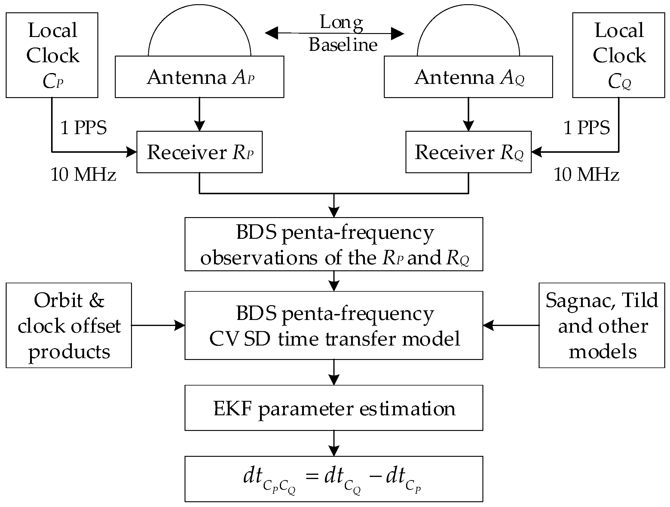
Figure 1 shows the implementation flow of PF SD time transfer. The remote GNSS timing receiver (RP and RQ) is connected to the remote local clock (CP and CQ) downwards and the remote GNSS antenna (AP and AQ) upwards, and the local clocks CP and CQ generate 1 PPS and 10 MHz signals to the remote GNSS timing receiver, RP and RQ. At this time, a long baseline time transfer link is formed between the receiver RP and RQ. After gross error and cycle slip detection by BDS PF code and phase observations, the correlation error can be eliminated or weakened by precision satellite orbit, satellite clock offset, ANTEX, code bias products and error models (for instance, the phase windup model, tides model and Sagnac model). At this time, based on the proposed BDS PF SD time transfer model, the local time difference or clock offset dtCPCQ can be obtained by parameter estimation using an extended Kalman filter (EKF), and then the goal of time transfer can be achieved.
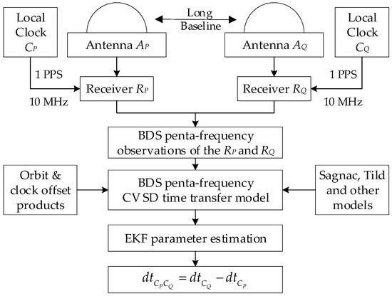
Figure 1.
Float chart of BDS penta-frequency SD time transfer.
3.2. Experimental Data Sources and Processing Methods
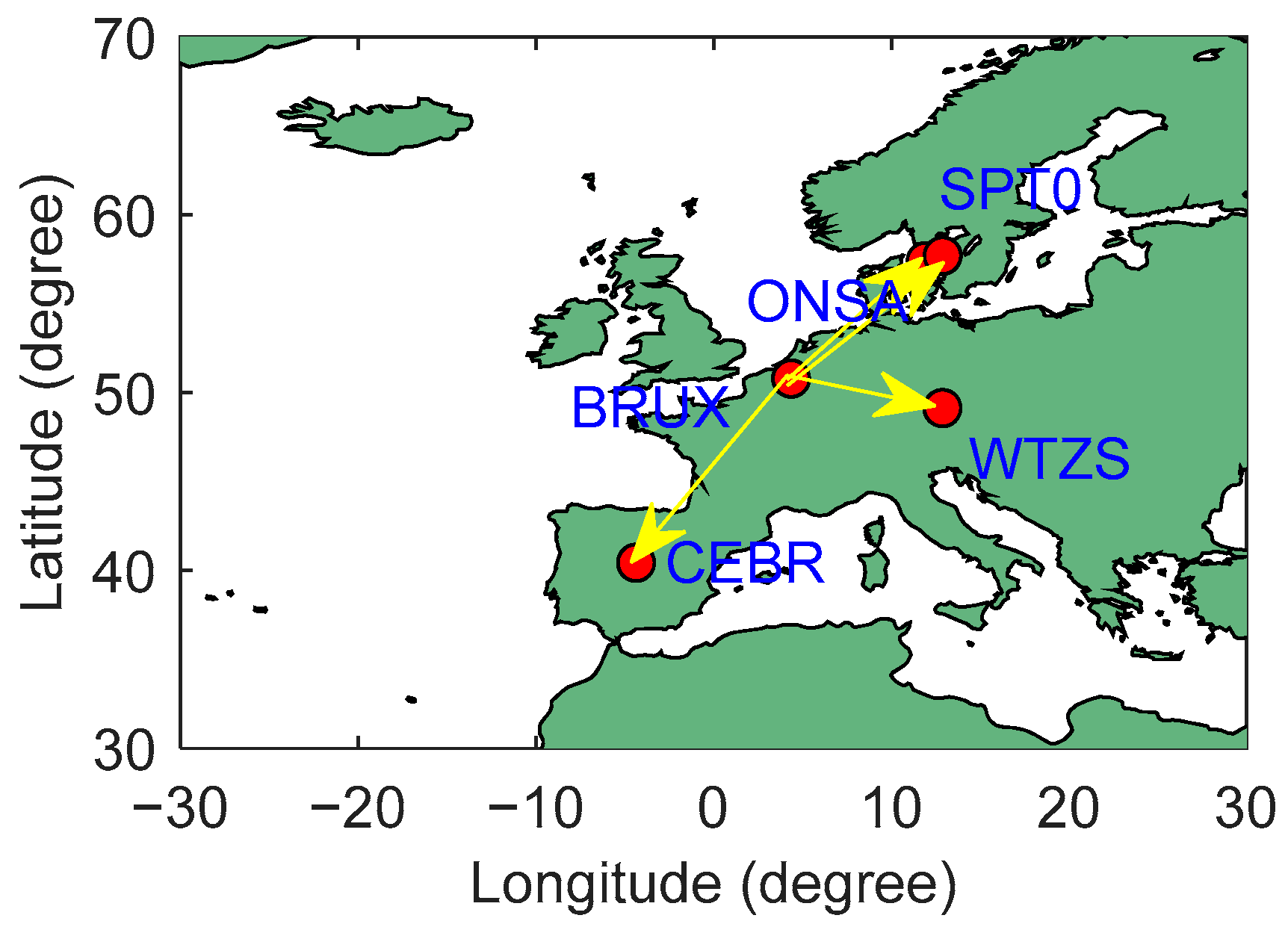
The BRUX, CEBR, ONSA, SPT0 and WTZS stations (equipped with Hydrogen-Maser (H-Maser) or Cesium-Maser (C-Maser)) support BDS B1C, B1I, B2a, B2b, B2I and B3I observations from the multi-GNSS experiment (MGEX) network, which was selected for PF CV SD time transfer experiment. Among these stations, the BRUX, SPT0 and WTZS refer to the Universal Time Coordinated (UTC) Punctuality Laboratory ORB (Observatoire Royal de Belgique), RISE (Research Institutes of Sweden AB) and IFAG (Institut für Angewandte Geodaesie), respectively. In addition, all the experimental stations are equipped with the same GNSS timing receivers (Septentrio PolaRx5TR), which helps to avoid the impact of receiver-type differences on time transfer results. The experiment period is the day of the year (DOY) 337 to DOY 343 in 2021, totaling one week. With BRUX as the central node, the BRUX-CEBR (1331.6 km), BRUX-ONSA (883.8 km), BRUX-SPT0 (947.4 km) and BRUX-WTZS (637.6 km) long baseline time links are established. Figure 2 and Table 2 show the geographical locations and basic information, respectively, of BRUX, CEBR, ONSA, SPT0 and WTZS stations.
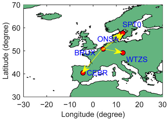
Figure 2.
Location distribution for BRUX, CEBR, ONSA, SPT0 and WTZS.
Table 2.
Stations information for BRUX, CEBR, ONSA, SPT0 and WTZS.
Table 3 illustrates the processing strategies for the BDS-3/BDS-2 combined PF SD time transfer. To simplify data processing, this research carries out equal weight processing between the B1C, B1I, B2a, B2b, B2I and B3I frequencies. The weight ratio of BDS-2 GEO, BDS-2 IGSO and MEO: BDS-3 satellites was set as 1:10:10 [39]. Considering that the experiment is in the ionospheric quiet period and the stations are all in the middle latitude, relevant studies [40] show that the high-order ionospheric delay in this case has little effect on the time transfer. Therefore, the IF combination is used in this study to eliminate the first-order term of ionospheric delay and ignore the impact of higher-order ionospheric delay. The modified GNSS open-source data processing software RTKLIB 2.4.3 b34 [41] (https://www.rtklib.com/, accessed on 10 April 2024) meets the needs of the BDS multi-frequency CV SD time transfer experiment. We use GeoForschungsZentrum (GFZ) rapid precise products and station coordinates fixed by IGS weekly solution file to perform the BDS-3-and-BDS-2 combined DF B1I and B3I IF combined PPP solution to evaluate the performance of SD solution. In addition, the Allan deviations (ADEV) are calculated to assess the frequency instability of the time transfer link.
Table 3.
Details of SD and PPP time transfer processing strategies.
4. Results
Firstly, we evaluated the number of satellites (NSats), time dilution of precision (TDOP) and multipath combination (MPC) noises of the experimental station. Next, the time transfer performance of four DF, nine TF and five QF SD models composed of BDS B1I, B2I, B2b, B3I, B1C and B2a observations were compared. Finally, the properties of IFB and time transfer stability of four PF SD models were evaluated.
4.1. Quality Analysis of BDS Multi-Frequency Observations
As shown in Figure 3, the NSats in the BDS-2/BDS-3 combination are significantly higher than those in BDS-2 and BDS-3. Compared with BDS-2, the BDS-3 NSats increased by 1.95 times, on average. The NSats of BRUX-CEBR, BRUX-ONAS, BRUX-SPT0 and BRUX-WTZS were 9.8, 12.4, 12.4 and 11.2, on average, respectively, and the corresponding TDOP values were 0.89, 0.75, 0.76 and 0.85, on average, respectively. The TDOP values of BRUX-CEBR and BRUX-WTZS were bigger than those of BRUX-ONSA and BRUX-SPT0 because of the poor quality of the CEBR and WTZS observations.
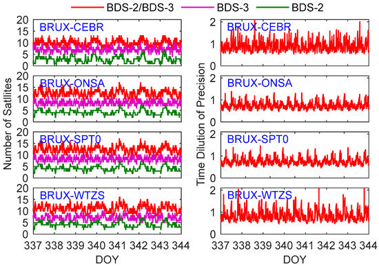
Figure 3.
The number of satellites (NSats) (left) and time dilution of precision (TDOP) (right) at BRUX-CEBR, BRUX-ONSA, BRUX-SPT0 and BRUX-WTZS links.
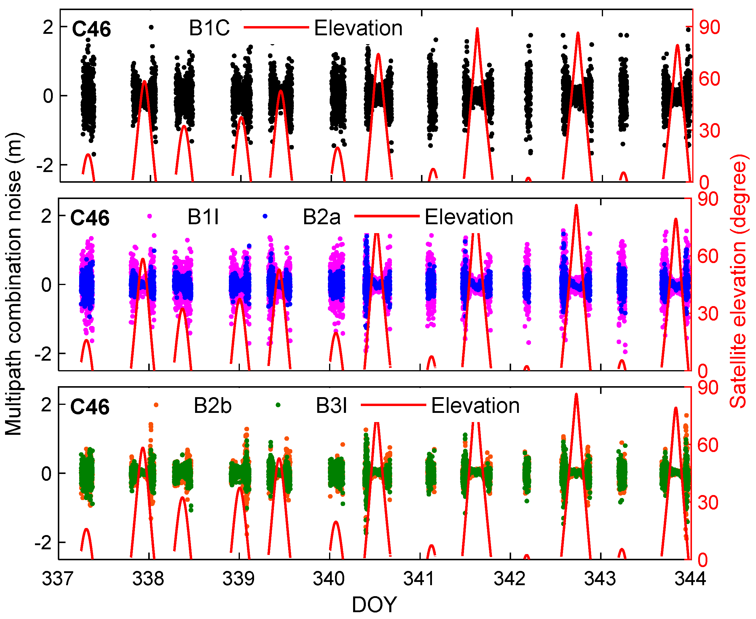
As shown in Figure 4, the MPC noises of each frequency are all within ±2.0 m. According to the statistics, the RMSs of B1C, B1I, B2a, B2b and B3I MPC noises are 0.347 m, 0.388 m, 0.222 m, 0.238 m and 0.220 m, on average. The B1I single has the highest MPC noise, and those of the B2a and Bb singles are similar. This indicates that BDS multi-frequency signals can provide higher-quality observations compared to traditional DF signals, making them more conducive to achieving high-precision time transfer. The average MPC noise of CEBR (0.356 m) is greater than in other stations (BRUX, ONSA, SPT0 and WTZS, which are 0.250 m, 0.254 m, 0.255 m and 0.299 m, respectively), and the B2a, B2b and B3I signals also reach 0.3 m, indicating that the data quality of CEBR is slightly poor.

Figure 4.
B1C, B1I, B2a, B2b and B3I frequencies multipath combination (MPC) noises at BRUX.
4.2. Performance Analysis of DF SD Time Transfer
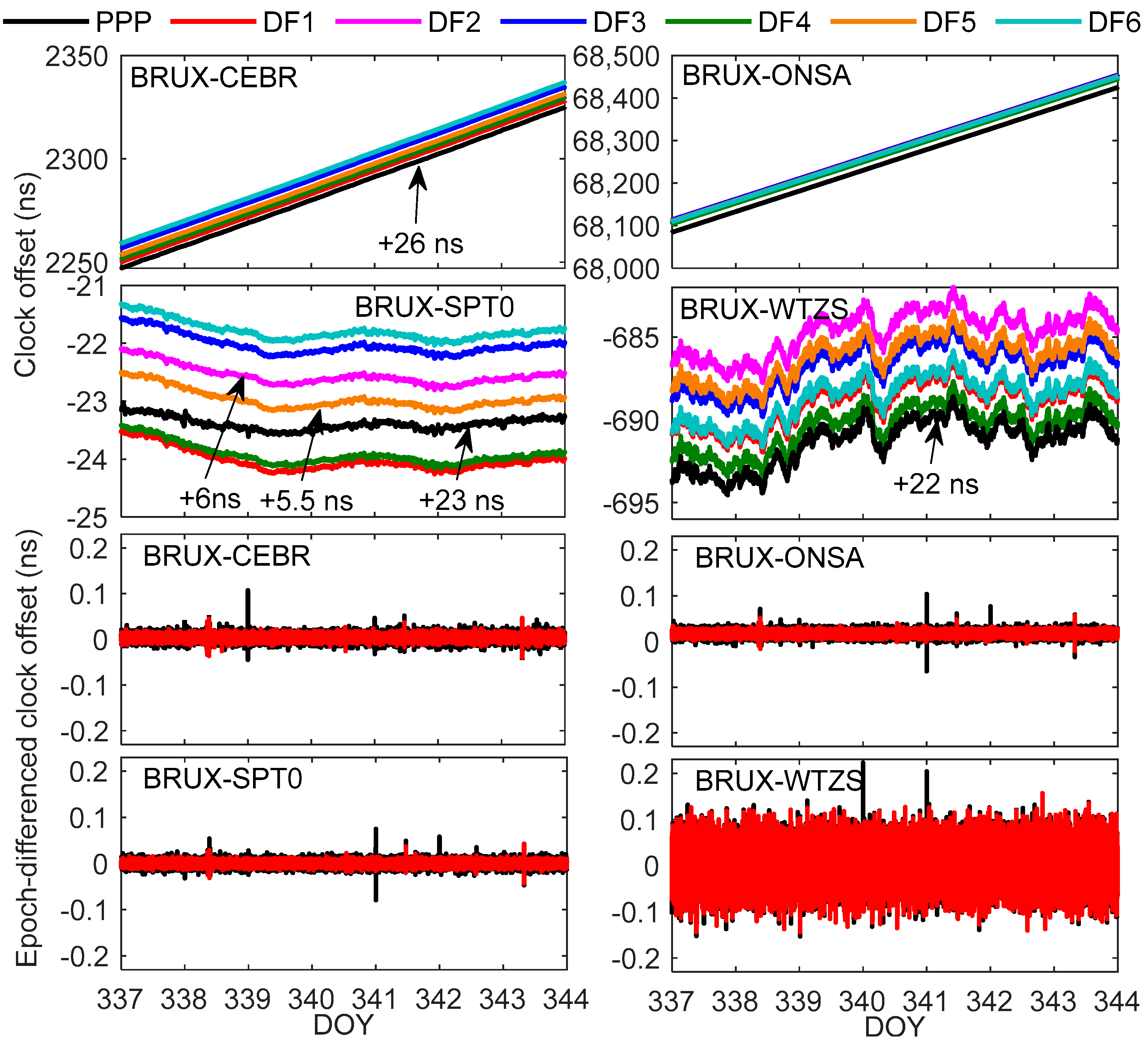
Figure 5 shows the results of the PPP and SD DF IF combined time transfer. Due to spatial limitations and the similarity between the SD time transfer results, Figure 5 only shows the results of the epoch-differenced clock offset for the PPP and SD DF1 models. It can be found that the time transfer results of the PPP, DF1, DF2, DF3, DF4, DF5 and DF6 models tend to be consistent, verifying the correctness of the established SD model. In particular, the clock offset variation amplitude of the BRUX-SPT0 and BRUX-WTZZ links is relatively small, which is related to the physical characteristics of the external clocks of the BRUX, SPT0 and WTZS stations. There are varying sizes of jumps in PPP at the daily boundary, and the jumps on each link are inconsistent (with a maximum value of about 0.1 ns). However, due to the weakening or elimination of the impact of daily boundary jumps in satellite clock offset products by the SD model, the time transfer results of SD are more stable compared to PPP, and these results are basically not affected by daily boundary jumps, which reflects the advantage of the SD model over the PPP model in time transfer. Furthermore, some of the jumps in non-daily boundary areas (such as around time 343.7) may be caused by the data quality of the satellite products or stations. In addition, due to the external clock of WTZS being a cesium clock, the epoch-differenced clock offset variation amplitude of the BRUX-WTZS link is slightly larger than in the other three links.
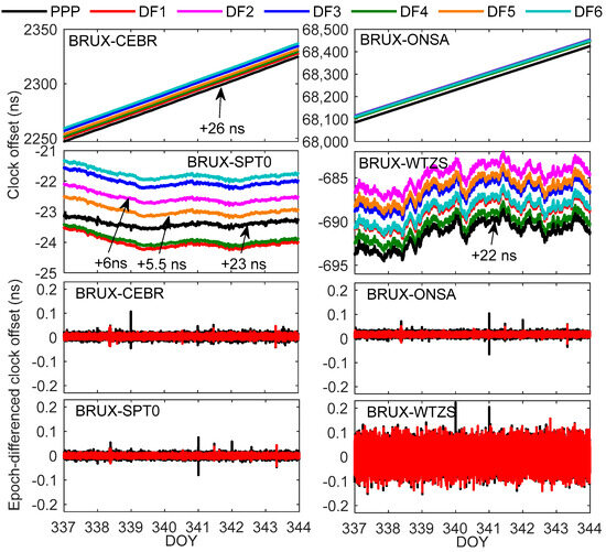
Figure 5.
Clock offset and epoch-differenced clock offset for the dual-frequency (DF) precise point positioning (PPP) and single-differenced (SD) time transfer results of the BRUX-CEBR, -ONSA, -SPT0 and -WTZ links formed in the experiment.
Figure 6 shows the difference between the time transfer results of the DF SD and PPP and the IGS final product. Since the differences between the schemes are small and have a certain overlap, the clock offset difference is shifted in this study to distinguish each scheme clearly. The variation trends of each DF model are entirely consistent. Due to the combination of different dual-frequency observations, the receiver clock offset will absorb different UCDs, resulting in a bias between the clock offsets of each DF model. The bias STDs between DF1, DF2, DF3, DF4, DF5 and DF6 are 18.6 ps, 16.4 ps, 11.6 ps, 14.2 ps and 11.6 ps, on average, respectively. These values prove that the biases between each DF SD model are very stable and meet the prerequisite for the time link calibration. The clock offset of each model has a jump at the daily boundary, caused by the IGS final product [54,55,56]. In addition, due to the loss of the CEBR clock offset provided by the IGS at some times, the result of the clock offset difference in the BRUX-CEBR link is discontinuous. We note that the clock offsets of SD are more stable than those of PPP, especially at the daily boundary (such as BRUX-WTZS in DOY 340), which is related to the SD algorithm’s weakening of satellite-related errors. By comparison, the fluctuation of the BRUX-CEBR clock offsets is significantly greater than in the other three links, which may be related to the fewer Nsats of BRUX-CEBR and the poor data quality of CEBR.
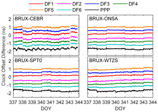
Figure 6.
Clock offset differences between the DF PPP and SD time transfer results of the BRUX-CEBR, -ONSA, -SPT0 and -WTZ links formed in the experiment and IGS reference value.
As shown in Table 4, the standard deviation (STD) values of the DF1, DF2, DF3, DF4, DF5 and DF6 solutions are basically the same. In order to reduce the impact of daily boundary jumps on accuracy evaluation, this study calculated the STD for each day and took the average of the STD as the result for the entire experimental period. Compared with PPP, the STDs of SD were reduced to different degrees, with maximum, minimum and average decreases of 48.2%, 25.3% and 36.5%, respectively, indicating that SD has apparent advantages in time transfer performance over PPP. In addition, compared with the traditional DF6 (B1I and B3I IF combination), the STD values of DF1, DF2, DF3, DF4 and DF5 also decreased, with maximum, minimum and average decreases of 18.8%, 0.4% and 8.0%, respectively, which is related to the smaller noise amplification coefficient of the DF1, DF2, DF3, DF4 and DF5 models. Among these models, the mean STD decrease of DF1 was the largest (9.8%), while that of DF3 was the lowest (3.3%), relating to the small noise amplification factor of DF1 and the large noise amplification factor of DF3. The mean STD reduction of BRUX-WTZS was the largest (15.5%), while BRUX-ONSA’s was the smallest (3.6%).
Table 4.
Standard deviation (STD) of the dual-frequency (DF) (SD) solutions when differenced from the IGS final product (ps).
As shown in Figure 7, in the BRUX-CEBR, BRUX-ONSA and BRUX-SPT0 links, the frequency stabilities of DF1, DF2, DF4 and DF5 are significantly improved compared with PPP before 30,000 s. The short-term frequency stabilities of DF3 and DF6 are close to those of PPP but slightly worse than those of DF1, DF2 and DF5 due to the significant noise amplification factor. The frequency stability of BRUX-SPT0 is the best, reaching about 1 × 10⁻¹⁵@1.2 × 10⁵ s. Due to the limited performance of the external cesium atomic clock of WTZS, the frequency stability of BRUX-WTZR is the worst (about 1 × 10⁻¹⁴@1.2 × 10⁵ s), and the frequency stability differences of PPP, DF1, DF2, DF3, DF4, DF5 and DF6 are small.
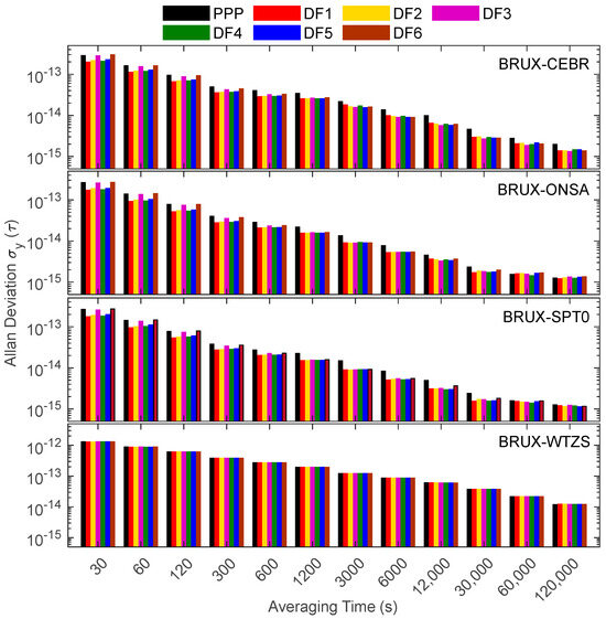
Figure 7.
Frequency instabilities of the four links formed in the experiment for the DF SD solution.
Figure 8 shows a specific difference (less than 1 × 10⁻¹²) in short-term frequency stability between the PPP and SD solutions, but there is little difference in the long-term frequency stability. DF1, DF2, DF4 and DF5 have smaller noise amplification factors, making their short-term frequency stability better than those of DF3 and DF6. The frequency stability of DF1, DF2, DF3, DF4 and DF5 was improved compared to that of PPP, but DF6 is still inferior to PPP at 30 s and 60 s, indicating the disadvantage of traditional B1I/B3I DF6 IF combinations compared to BDS new signal IF combinations. Compared with DF PPP and DF6, the multi-frequency DF solutions’ stabilities are increased by 6.5% and 2.7%, on average, proving the advantage of multi-frequency in SD time transfer. It should be noted that the fluctuation (1200 s to 30,000 s) in the stability increase in DF compared to PPP is due to the influence of the PPP frequency stability of the BRUX-CEBR link.
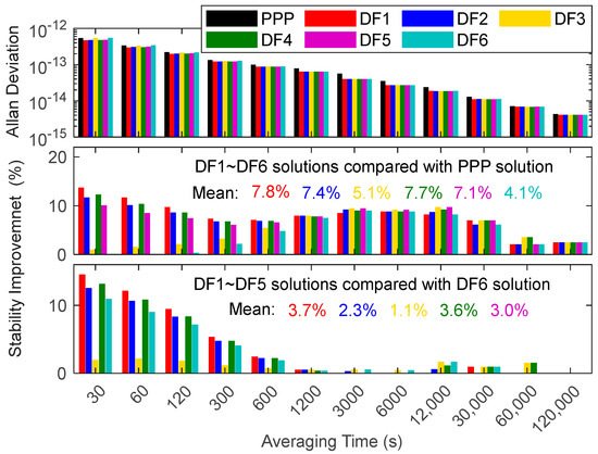
Figure 8.
Average frequency instability for DF SD solution and the improvement rate of frequency stability for DF SD solution.
4.3. Performance Analysis of TF SD Time Transfer
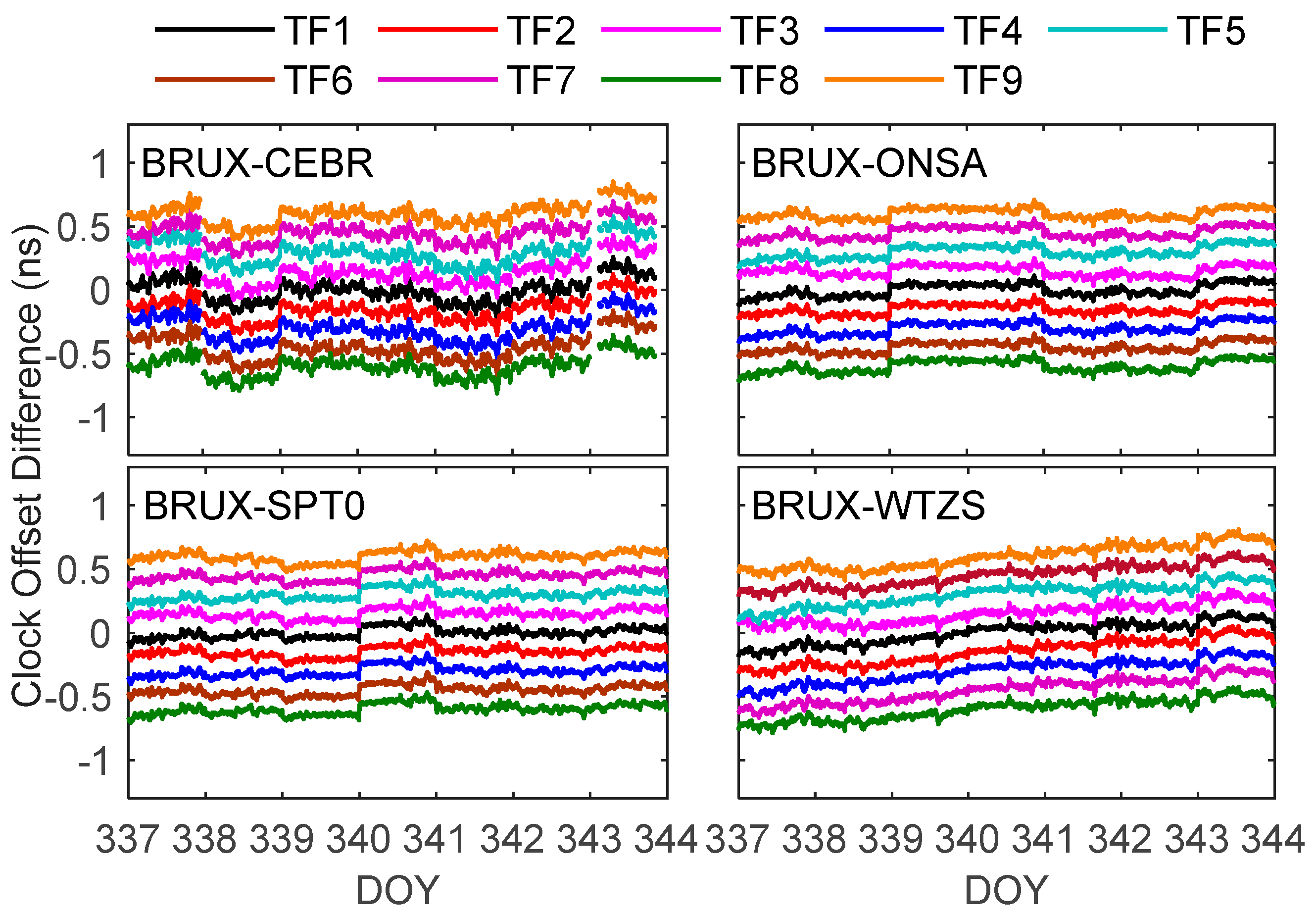
Figure 9 shows that the variation trends of the nine SD TF situations were roughly the same. The bias STDs between TF2, TF3, TF4, TF5, TF6, TF7, TF8, TF9 and TF1 solutions are 7.7 ps, 14.2 ps, 6.0 ps, 5.7 ps, 9.7 ps, 6.7 ps, 6.1 ps and 11.0 ps, on average. These values indicate that the bias was stable and met the prerequisite for the time link calibration for each TF SD model. By combining Figure 5 and Figure 7, it can be observed that the clock offset trends of the SD TF and DF are consistent, confirming the correctness of the SD TF time transfer model.
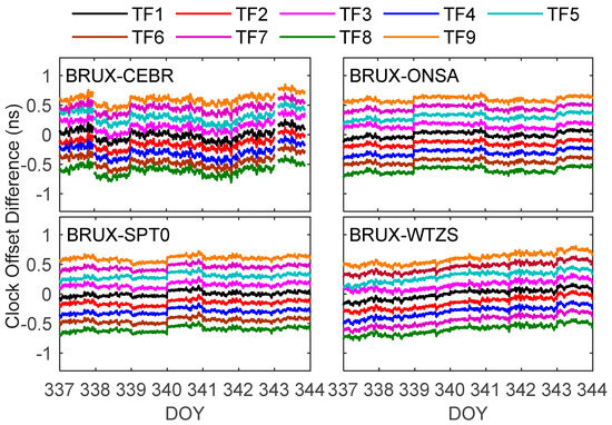
Figure 9.
Clock offset differences between the triple-frequency (TF) SD time transfer results of the BRUX-CEBR, -ONSA, -SPT0 and -WTZ links formed in the experiment and IGS reference value.
As shown in Table 5, the STD of each TF model is basically the same. Compared with the DF6, the STD of each TF model is also decreased, with maximum, minimum and average decreases of 16.5%, 3.4% and 9.1%, respectively. Specifically, the mean decrease rate of TF1 was the largest (9.9%), while that of TF9 (7.6%) was the lowest. To better reflect the advantages of multi-frequency, we also compared the results of multi-frequency SD and DF PPP in the following study. Compared with the DF PPP, the mean STD’s TF reduction rate (38.1%) is higher than that of DF (36.5%), proving the advantage of the TF observations.
Table 5.
STD values of the BDS-3/BDS-2 combined triple-frequency (TF) SD solutions when differenced with the IGS final receiver clock offset product (ps).
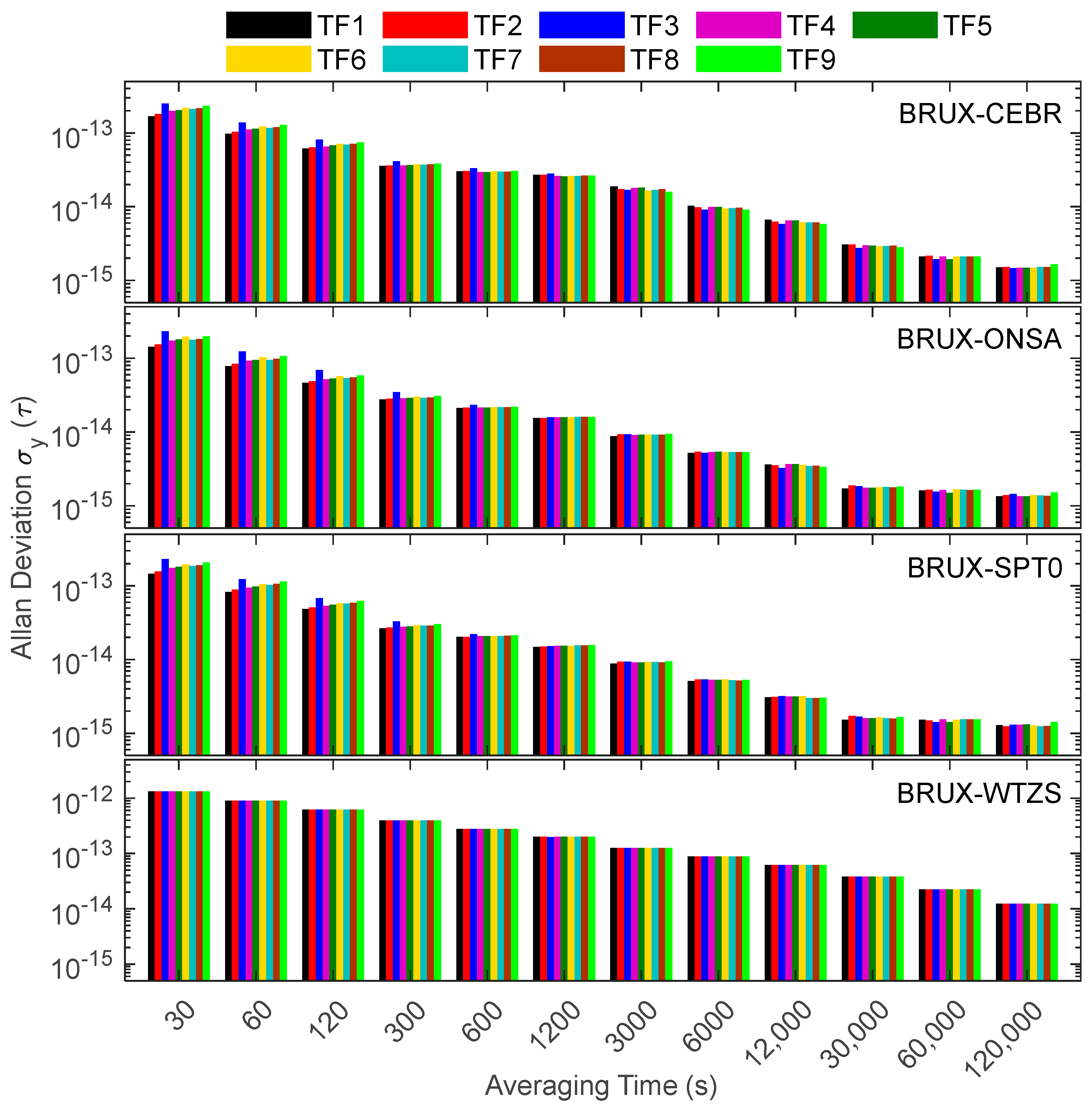
As shown in Figure 10, the significant difference in noise among various TF models (with a maximum value of 0.8) resulted in a slight difference in the short-term frequency stability. In particular, the short-term frequency stability of TF1 is the best, and that of TF3 is the worst, which is related to the minimum noise coefficient of TF1 and the maximum noise coefficient of TF3. However, with the increase in the averaging time, the influence of noise gradually decreases. Furthermore, limited by the accuracy of phase observations, the long-term frequency stability levels of each TF model are similar. In addition, there is no significant difference in the frequency stability of each TF model in the BRUX-WTZS link, which is related to the poor clock performance of the WTZS.
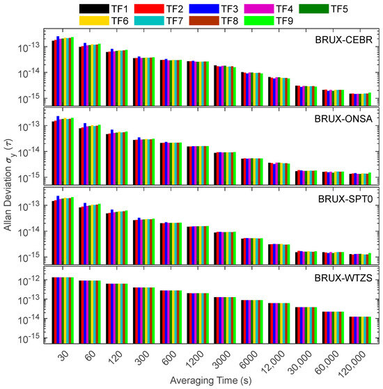
Figure 10.
Frequency instabilities of the four links formed in the experiment for TF SD solutions.
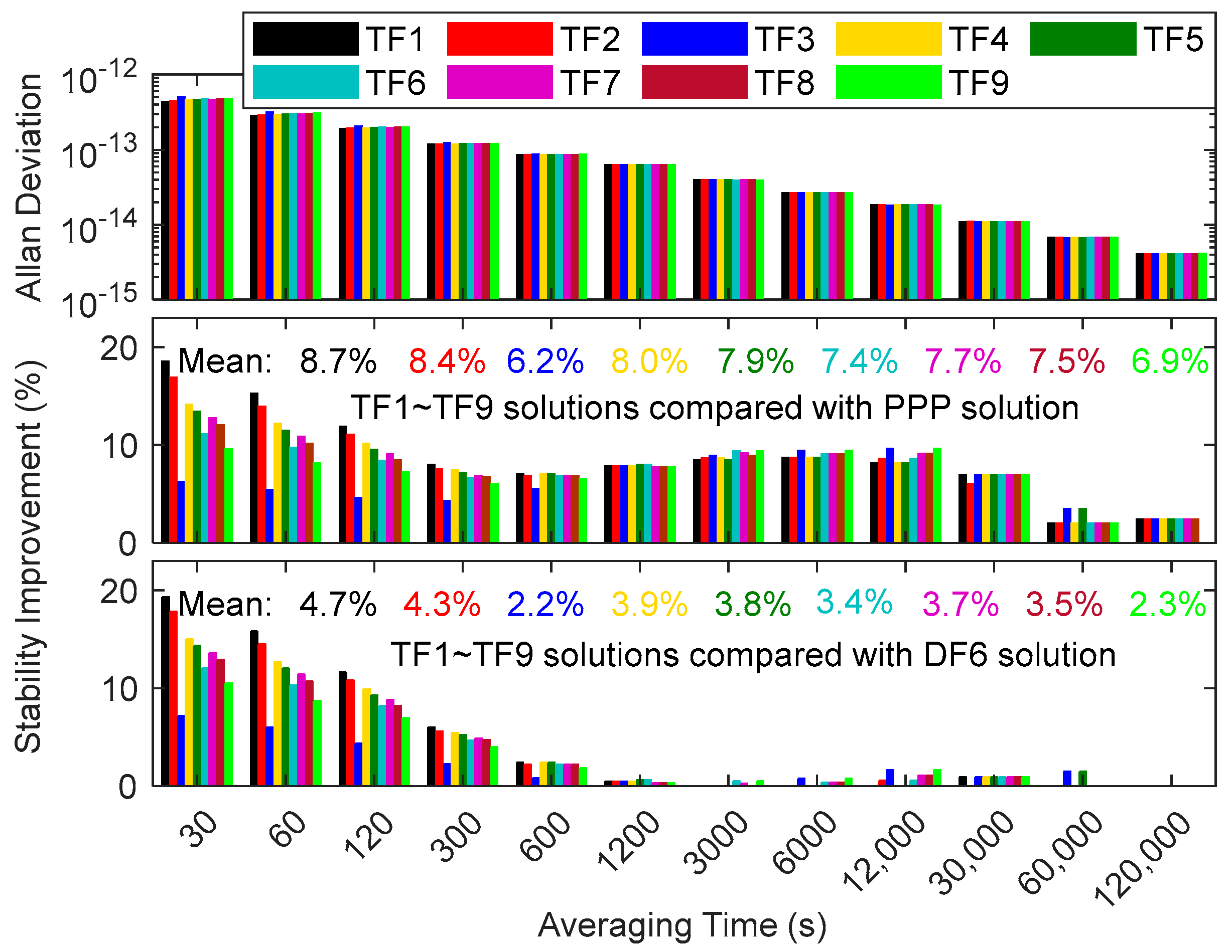
Figure 11 shows small differences (less than 1 × 10⁻¹³) in short-term frequency stability (especially before averaging time 300 s) between each of the TF models. However, the long-term frequency stability is the same (especially after an averaging time of 12,000 s). TF1 and TF2 have smaller noise amplification factors, making their corresponding short-term frequency stability better than those of the other TF models. Overall, TF1 has the best frequency stability, while TF3 has the worst. Compared with the DF PPP, TF’s frequency stability improvement (7.6%) is higher than that of DF (6.5%), on average. The TF1 (which has the best frequency stability in the TF model) has a 1% increase in stability compared to DF1 (which has the best frequency stability in the DF model), proving the TF signal’s small advantage in timing over the DF signal.

Figure 11.
Average frequency instability for TF SD solution and the improvement rate of frequency stability for TF SD solution.
4.4. Performance Analysis of QF SD Time Transfer
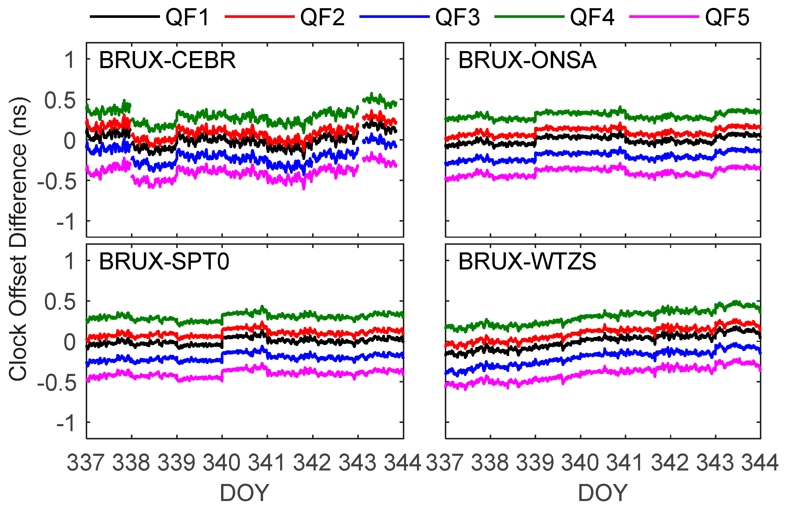
Figure 12 shows that the variation trends of the QF1, QF2, QF3, QF4 and QF5 clock offsets are roughly the same. The bias STDs between QF2, QF3, QF4, QF5 and QF1 are 2.8 ps, 6.2 ps, 6.0 ps and 6.2 ps, on average, respectively. The mean STD of the QF (the mean value is 5.3 ps) is smaller than those of the DF (the mean value is 14.5 ps) and TF (the mean value is 8.4 ps), which means that the consistency of the QF models is better than that of the DF and TF models. Compared to Figure 5 and Figure 7, the results of the QF are consistent with those of the DF and TF, indicating there may be no significant improvement in the accuracy of QF compared to DF and TF.

Figure 12.
Clock offset differences between the quad-frequency (QF) SD time transfer results of the BRUX-CEBR, -ONSA, -SPT0 and -WTZ links formed in the experiment and IGS reference value.
As shown in Table 6, the STD of each QF model is basically the same (the maximum and minimum difference in the same link are about 1.44 ps and 0.02 ps, respectively). Compared with the DF6, the STD of each QF model is reduced, with maximum, minimum and average decreases of 3.4%, 16.6% and 10.0%, respectively. The mean STD decrease rate of QF1 was the most significant (11.1%), while that of QF3 was the lowest (9.2%). Compared with the DF PPP, the STD values of the five QF models were all decreased, with maximum, minimum and average decreases of 48.8%, 33.6% and 38.8%, respectively. The reduced ratio in the QF STD (38.8%) was higher than that of the DF (36.5%) and TF (38.1%), which proves the advantage of the QF.
Table 6.
STD values of the quad-frequency (QF) SD solutions when differenced from the IGS final receiver clock offset product (ps).
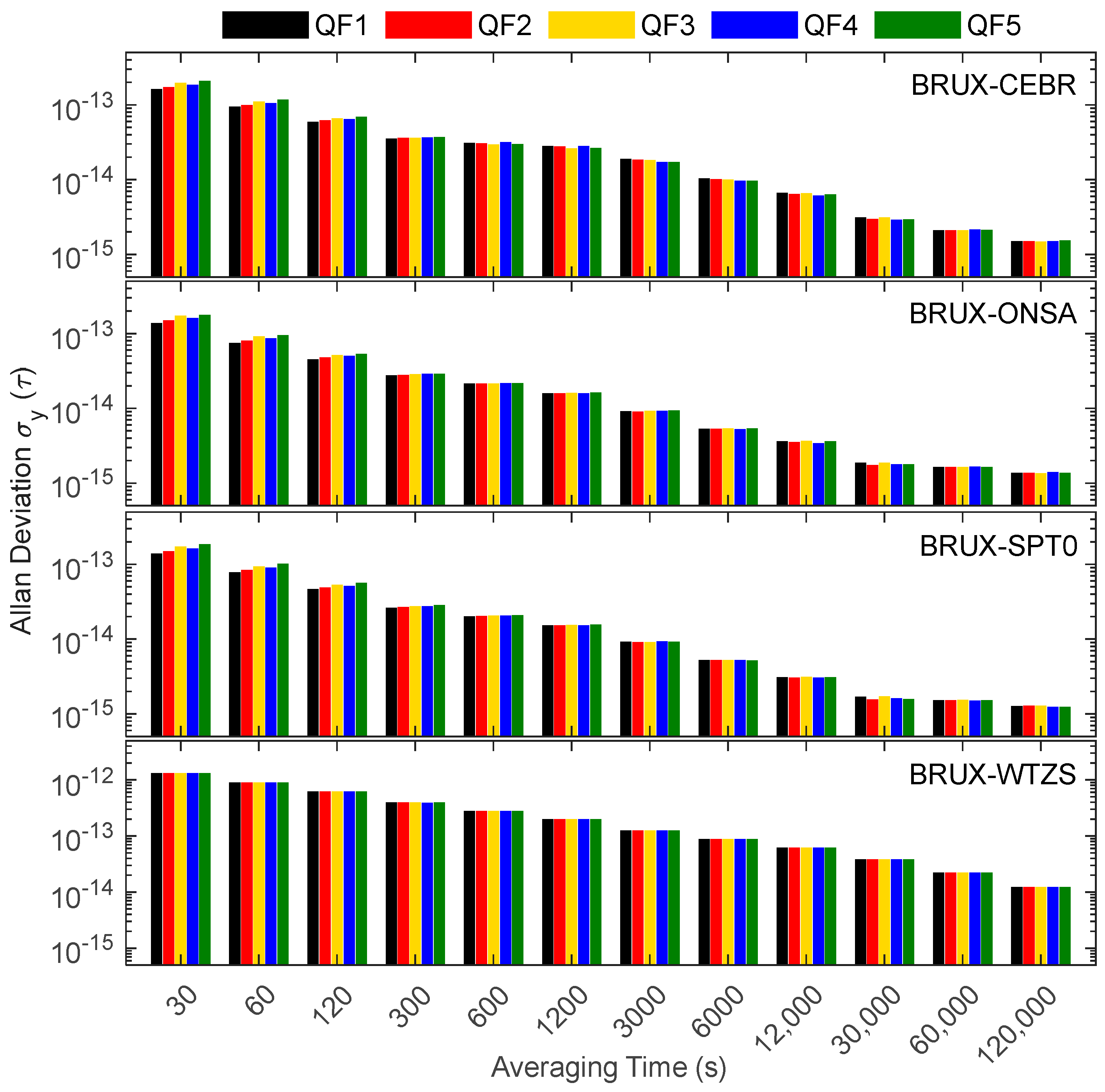
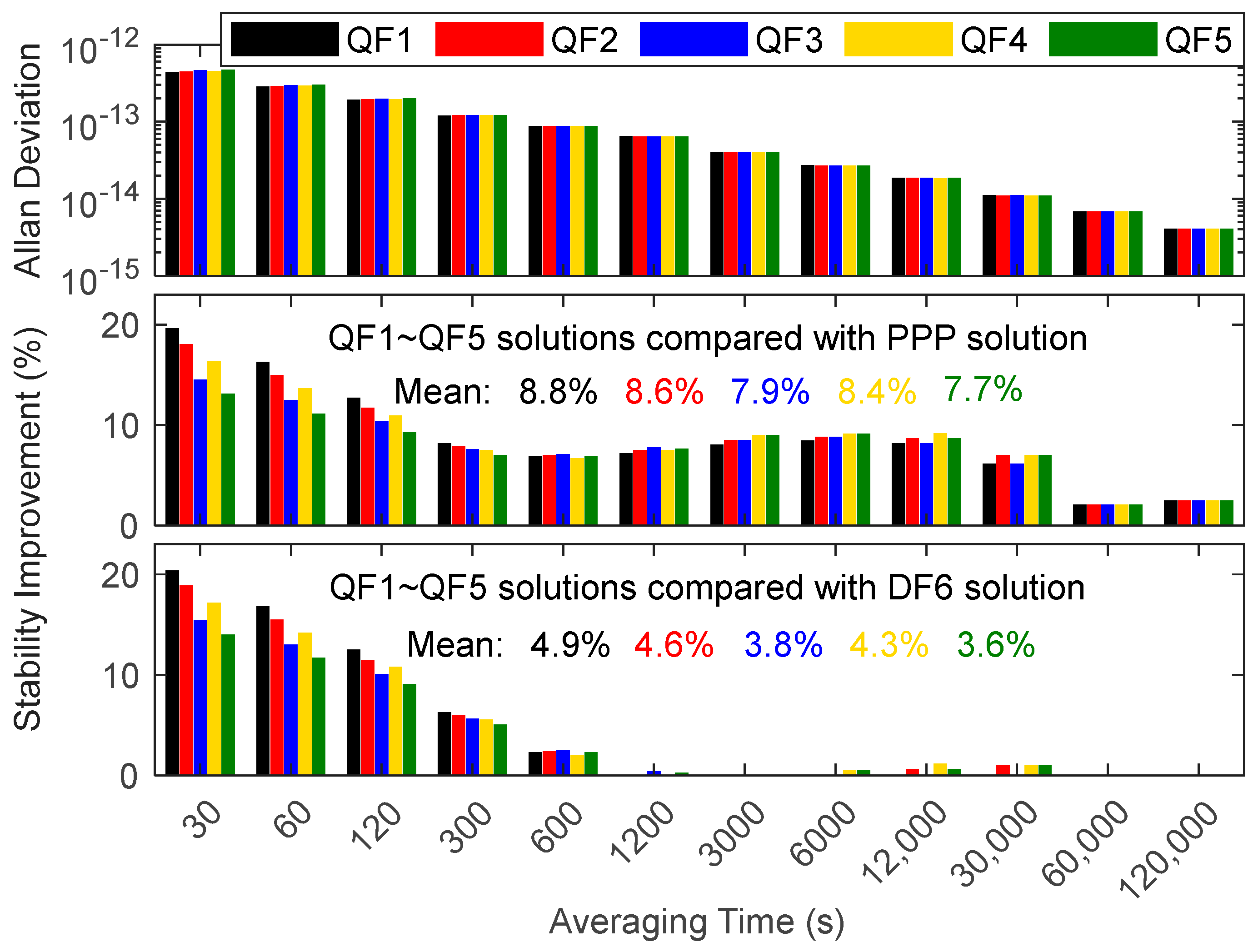
Figure 13 and Figure 14 show some differences (of less than 1 × 10⁻¹²) in short-term frequency stability among the QF1, QF2, QF3, QF4 and QF5 models. However, the long-term frequency stability of those models is basically the same (especially if the averaging time exceeds 6000 s). The short-term frequency stability of QF1 is the best, and that of QF5 is the worst, which is related to the minimum noise factor of QF1 and the maximum noise factor of QF3. With the increase in the averaging time, the influence of noise on time transfer gradually decreases, resulting in the long-term frequency stabilities of each QF model being similar. Overall, QF1 and QF2 have the best frequency stability, while QF5 has the worst. By comparison with DF PPP, the frequency stability of an improved rate of QF (8.3%) is higher than those of DF (6.5%) and TF (7.6%), on average. In addition, by comparison with DF6, the mean value of the frequency stability improvement rate of QF (4.2%) is higher than those of DF (2.7%) and TF (3.5%), which proves the advantage of QF over DF and TF in timing.
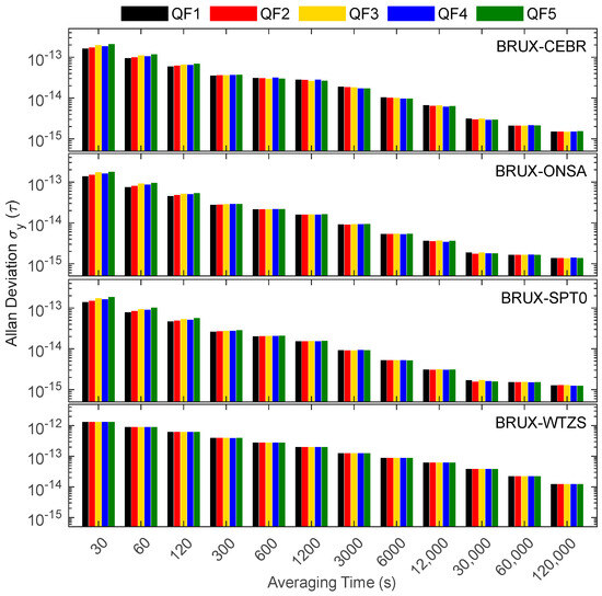
Figure 13.
Frequency instabilities of the four links formed in the experiment for QF SD solutions.

Figure 14.
Average frequency instability for QF SD solution and the improvement rate of frequency stability for QF SD solution.
4.5. Performance Analysis of PF SD Time Transfer
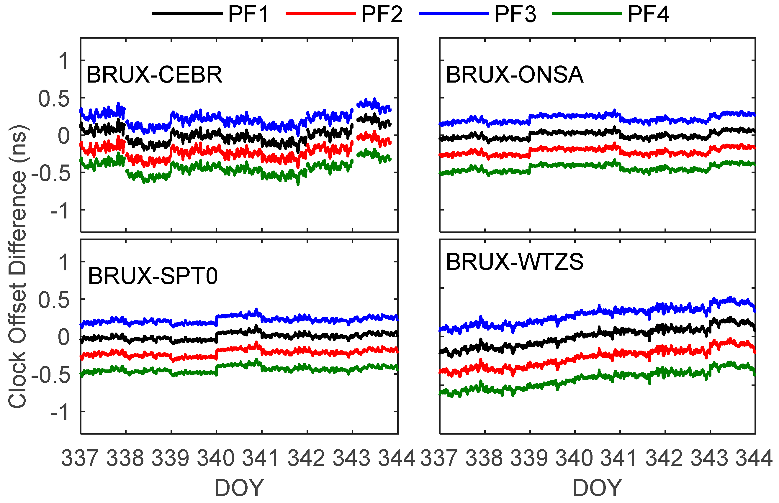
As shown in Figure 15, the variation trends of each PF model are roughly the same. The bias STDs between PF1, PF2, PF3 and PF4 are 7.2 ps, 6.7 ps and 6.0 ps, on average, respectively. The average STD of the PF (6.6 ps) is smaller than those of the DF (14.5 ps) and the TF (8.4 ps) but bigger than that of the QF (5.3 ps). This phenomenon may be related to the stability of IFB parameters estimated by PF1, PF2 and PF3 models.

Figure 15.
Clock offset differences between the penta-frequency (PF) SD time transfer results of the BRUX-CEBR, -ONSA, -SPT0 and -WTZS links formed in the experiment and IGS reference value.
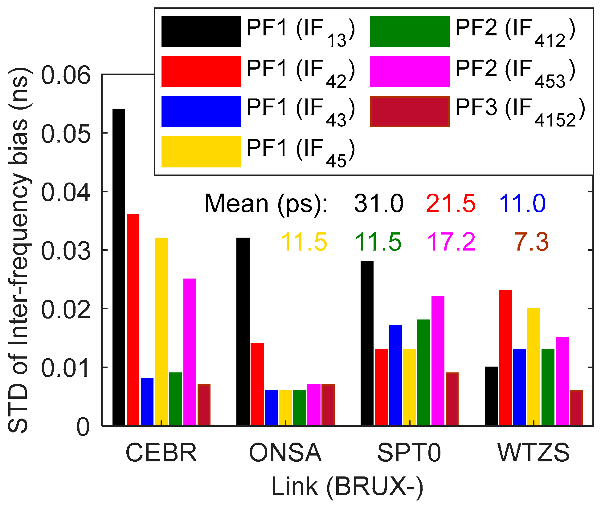
As shown in Figure 16, the maximum of IFB reaches 10.0 ns, the minimum is only 0.2 ns and IFB is a relatively stable parameter. The STD of PF1 (IF13) is the largest, which may be related to the small number of satellites in BDS-2. The STD of PF1 (22.3 ps) is greater than that of PF2 (14.4 ps), while the STD of PF2 is greater than that of PF3 (7.3 ps). Since IFB is strongly correlated with receiver clock offsets, the stability of IFB will directly affect the performance of timing, which means that the PF3 time transfer performance will be better than those of PF1 and PF2.
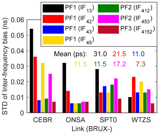
Figure 16.
STD values of single-differenced inter-frequency bias (IFB) at BRUX-CEBR, -ONSA, -SPT0 and -WTZS links for PF1, PF2 and PF3 CV SD solutions.
As shown in Table 7, the STDs of PF1, PF2, PF3 and PF4 are 23.4 ps, 23.2 ps, 23.0 ps and 22.6 ps, on average, respectively. The PF4 has the smallest STDs, and with the increase in IFB to be estimated, the STDs gradually increase, which is related to the accuracy of the estimated IFB. Combining Figure 14 and Table 7, it can be seen that PF3’s time-transfer STD is better than PF2’s, and PF2’s time-transfer STD is better than PF1’s, which corresponds to the STD of PF1, PF2 and PF3 IFB parameters, and further proves that there is a strong correlation between IFB and receiver clock offset. Compared with the traditional DF6, the STDs of the four PF models are decreased, with maximum, minimum and average decreases of 4.8%, 18.5% and 9.8%, respectively. Specifically, the mean decrease rate of PF4 was the largest (11.4%), while that of PF1 was the lowest (8.5%). Compared with the DF PPP, the STDs of each PF model are decreased, with maximum, minimum and average decreases of 48.9%, 33.0% and 38.7%, respectively. We found that the mean STD reduced ratio of PF4 (39.8%) is slightly higher than those of DF1 (36.5%), TF1 (38.1%) and QF1 (39.5%), which proves the slight advantage of the penta-frequency.
Table 7.
STD values of the PF SD solutions when differenced from the IGS final product (ps).
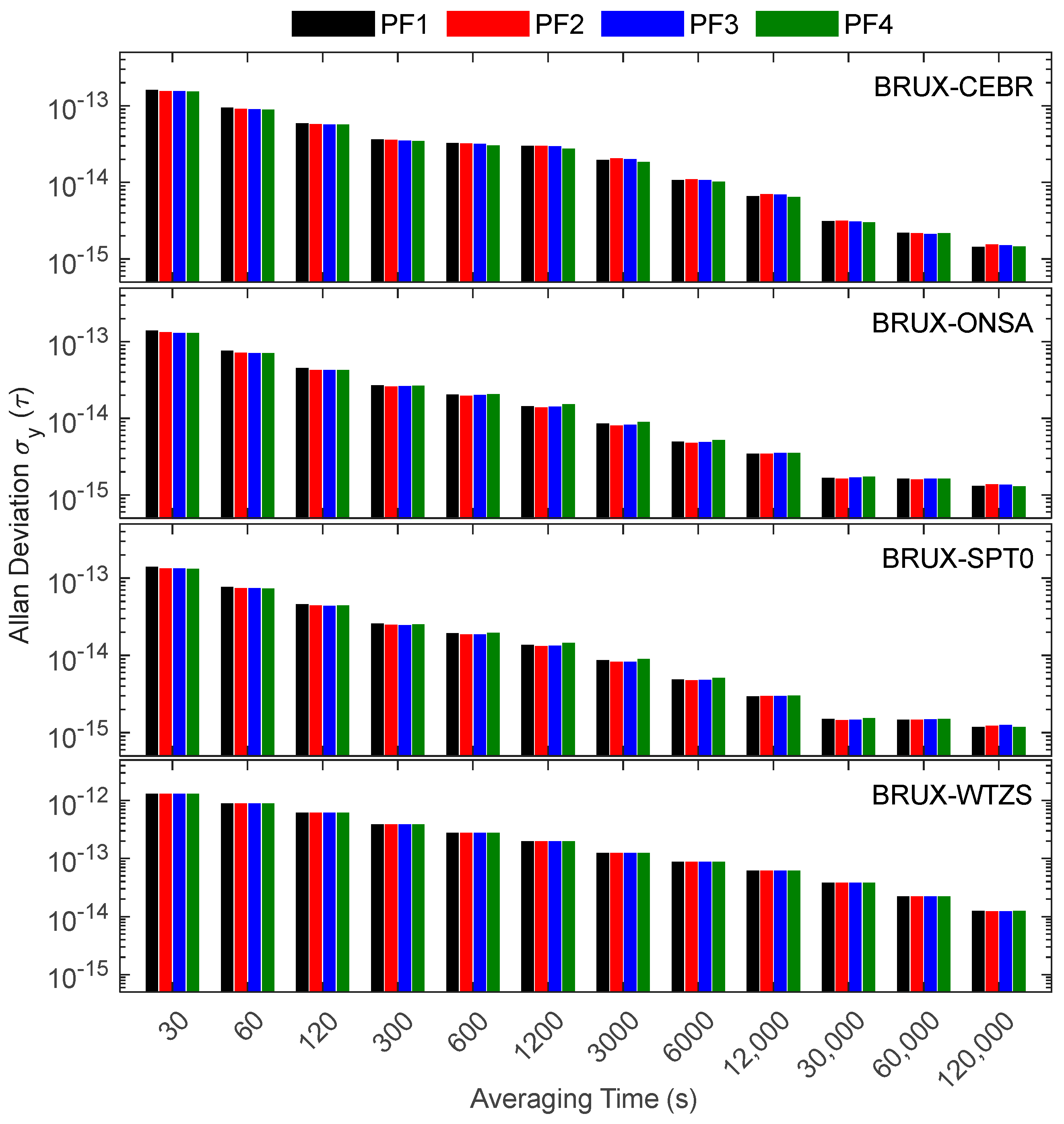
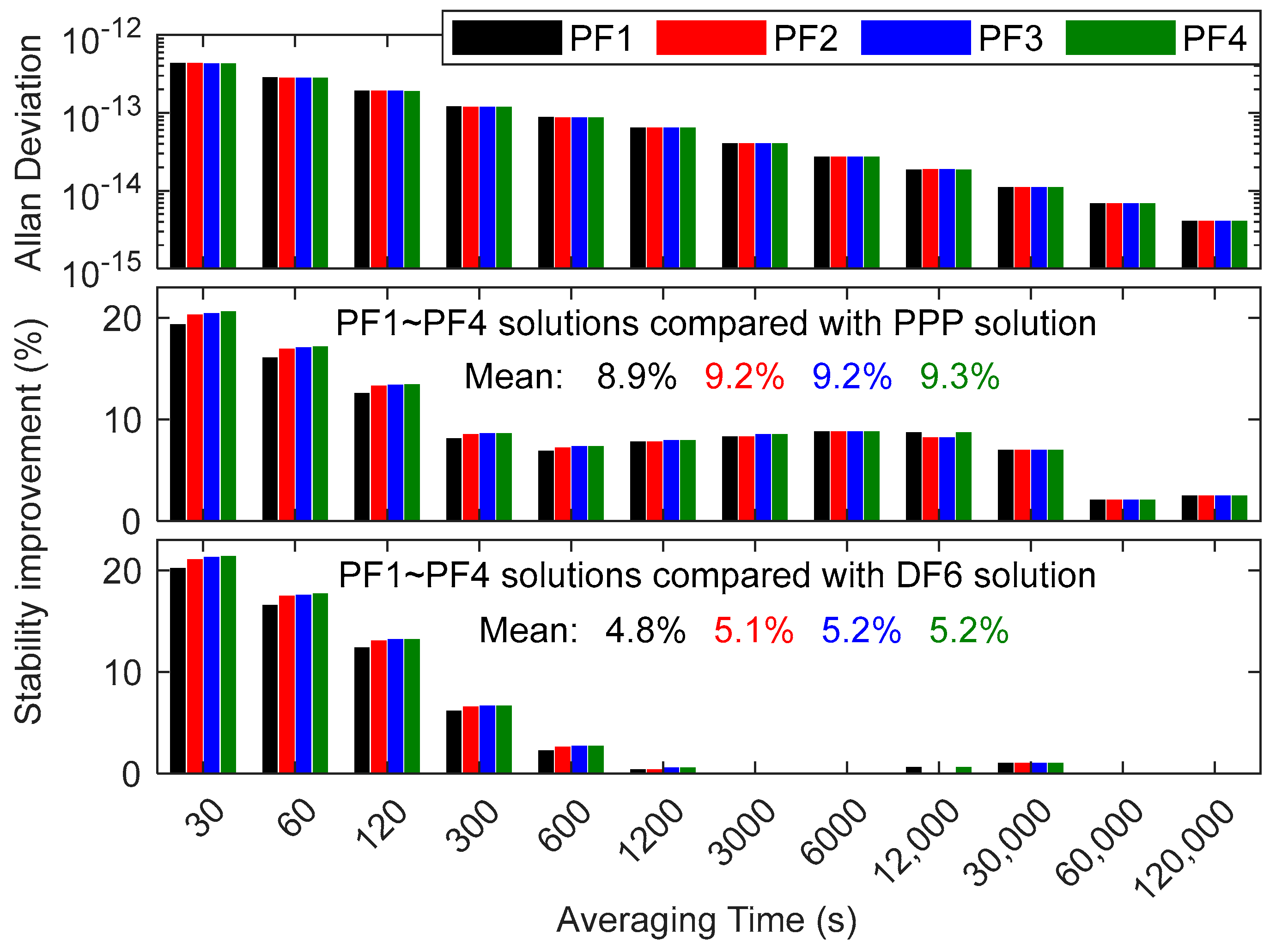
Figure 17 and Figure 18 show the frequency instability of the PF1-PF4 models for four-time links. It can be found that the frequency stabilities of the PF1-PF4 models tend to be consistent (the stability difference is less than 1 × 10⁻¹³@30 s). Especially when the averaging time exceeds 3000 s, the frequency stability is the same. The PF4 model’s short-term frequency stability is better than those of the PF1, PF2 and PF3 models because it does not need to estimate additional IFB parameters. Overall, PF4 has the best frequency stability, while PF1 has the worst. Although the flexibility of the PF1, PF2 and PF3 models is better than that of the PF4 model, the stability levels of PF1, PF2 and PF3 are slightly worse than that of the PF4 due to the additional estimation of IFB. Considering that the noise amplification factor of the PF4 is less than those of PF1, PF2 and PF3, we recommend the PF4 for PF time transfer and the use of PF2, PF2, or PF3 to supplement the PF4 in cases of PF data loss. Compared with the DF PPP, the mean frequency stability improvement rate of PF (9.2%) is higher than those of DF (6.5%), TF (7.6%) and QF (8.3%). Compared with the DF6, the frequency stability improvement rate of PF4 (the best frequency stability in the PF model) is increased by 1.5%, 0.6% and 0.3% over DF1 (the best frequency stability in the DF model), TF1 (the best frequency stability in the TF model) and QF1 (the best frequency stability in the QF model), on average, which proves the slight advantage of PF in time transfer compared with DF, TF and QF.

Figure 17.
Frequency instabilities of the four links formed in the experiment for PF SD solutions.
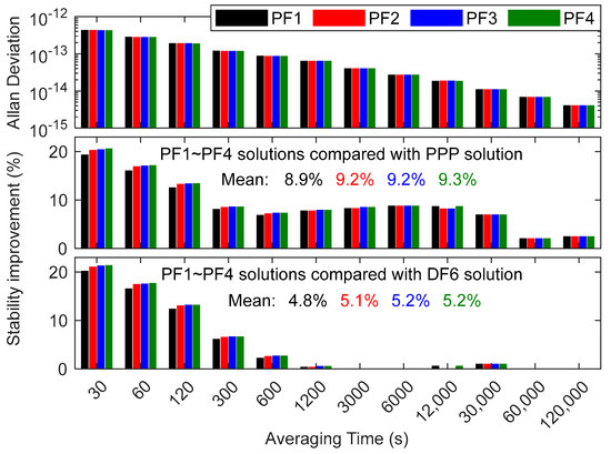
Figure 18.
Average frequency instability for PF SD solution and the improvement rate of frequency stability for PF SD solution.
5. Discussion
This research establishes an SD time transfer model with BDS PF observation and verifies the accuracy and reliability of the proposed DF, TF, QF and PF SD models through experiments. The noise amplification factor of a multi-frequency IF combination is smaller than that of a traditional DF IF combination, and as the number of signals increases, the noise amplification factor shows a gradually decreasing trend. The reduction in the noise amplification factor significantly improved the accuracy and short-term stability of SD time transfer. However, limited by the accuracy of carrier phase observations, the long-term stability of the multi-frequency SD model does not show significant improvement compared to the DF SD model. Therefore, it will still be worth studying how to use BDS multi-frequency signals to improve the long-term stability of SD time transfer in the future. It is worth noting that the weight ratio between multi-frequency observations is also an important factor affecting the accuracy of multi-frequency SD time transfer, and the reasonable weighting of multi-frequency observations is still worth exploring.
Moreover, due to the difficulty of achieving precise separation in receiver clock offset and ambiguity parameters in SD float solutions, and because of the failure to utilize the integer characteristics of ambiguity parameters, the accuracy of SD time transfer may be affected. Considering that there are too many types of IF combinations of multi-frequency signals, the noise of the IF combination is amplified by, at least, about two times, and various types of IF combinations will inevitably create a certain pressure when fixing ambiguity. Therefore, future research will focus on BDS multi-frequency un-combined SD time transfer and fix multi-frequency un-combined SD ambiguity to improve the performance of SD time transfer.
Furthermore, although the PPP time transfer model has a wider range of tasks compared to the SD time transfer model, SD time transfer still has certain advantages, especially in real-time processing, short baselines and network solutions, in which the benefits of that model and its accuracy are more pronounced. Therefore, the research and evaluation of multi-frequency SD time transfer models are necessary and have strong practical significance.
6. Conclusions
In this research, BDS-3/BDS-2 combined PF IF combination CV SD time transfer models with B1I, B3I, B2I, B1C, B2a and B2b signals were established, and the BRUX, CEBR, ONSA, SPT0 and WTZS stations, which are equipped with atomic clocks, were selected to establish four time-links for the experiment. The time transfer accuracy and frequency stability of the BDS DF, TF, QF and PF IF combination SD models were evaluated.
The results demonstrate that the multi-frequency SD time transfer accuracy and frequency stability can research sub-ns and about 1 × 10⁻¹⁵@120,000 s, respectively. The time transfer performance of SD is slightly better than that of PPP. The accuracy of multi-frequency SD time transfer is higher than that of traditional dual-frequency (B1I and B3I IF combination), with the STD and stability decreased by 5.9% and 4.0%, on average. This is especially due to the reduction in noise after multi-frequency IF combination, which significantly improves the short-term frequency stability of multi-frequency. However, limited by the accuracy of the observations, the frequency stability improvement of multi-frequency compared to DF is relatively limited. It is interesting that as the number of IF combined signals increases, the performance of the time transfer also steadily and slowly improves, and the performance of PF is slightly higher than those of other multi-frequency models (the stability of PF increased by 2.5%, 5.3% and 8.5% compared to DF, TF and QF, respectively), demonstrating the advantages of multi-frequency signals. Moreover, the DF1 (B1C and B2a DF IF combination), TF1 (B1C, B2a and B2b TF IF combination), QF1 (B1C, B1I, B2a and B2b QF IF combination) and PF4 (B1C, B1I, B2a, B2b and B3I PF IF combination) SD models have better performance in timing, and the PF4 SD model has the best performance. It is worth noting that the time transfer performance of PF1, PF2 and PF3 is slightly worse than that of PF4 due to the stability of the additional estimation of IFB parameters. Considering that the PF4 SD model does not require an estimate of IFB and that its noise factor is minor compared with the PF1, PF2 and PF3 SD models, we recommend the PF4 SD model (with PF signals to form a single IF observation equation) for multi-frequency time transfer and the use of the PF2, PF2 or PF3 SD model to supplement the PF4 SD model in cases of penta-frequency observation loss.
Since the four major global GNSS have supported at least triple-frequency signals and the advantages of the SD model in short baseline, real-time and network solutions, the SD time transfer technology of multi-frequency signals will expand the application of GNSS in the field of time and frequency measurement, which is of great significance for promoting the development of time and frequency measurement technology.
Author Contributions
Conceptualization, W.X. and W.S.; methodology, L.L. and C.Y.; software, W.X. and L.L.; validation, W.X., P.Z., C.Y. and L.W.; formal analysis, W.X.; investigation, W.X.; resources, C.Y.; data curation, L.W.; writing—original draft preparation, W.X. and L.L.; writing—review and editing, C.Y. and L.W.; visualization, W.X., P.Z. and J.S. All authors have read and agreed to the published version of the manuscript.
Funding
This work is supported by the National Natural Science Foundations of China (No. 42030105; No. 42204091; No. 42304095), the China Postdoctoral Science Foundation (No. 2024M752480), the Key Project of Natural Science Research in Universities of Anhui Province (No. 2023AH051634; No. 2024AH051436), and the Chuzhou University Research Initiation Fund Project (No. 2023qd07, No. 2023qd08).
Data Availability Statement
The BDS-2 and BDS-3 multi-frequency observations are available at ftp://igs.gnsswhu.cn/pub/gps/data/daily/, accessed on 20 August 2024.
Acknowledgments
We thank the IGS for providing precise satellite orbit and satellite clock offset products and BDS observations used in this research. We also thank Tomoji Takasu for providing RTKLIB (2.4.3 b34) open-source software.
Conflicts of Interest
The authors declare no conflict of interest.
References
- Yang, Y.; Li, J.; Xu, J.; Tang, J.; Guo, H.; He, H. Contribution of the Compass satellite navigation system to global PNT users. Chin. Sci. Bull. 2011, 56, 2813–2819. [Google Scholar] [CrossRef]
- Yang, Y.; Tang, J.; Montenbruck, O. Chinese navigation satellite systems. In Springer Handbook of Global Navigation Satellite Systems; Springer: Cham, Switzerland, 2017; pp. 273–304. [Google Scholar]
- Yang, Y.; Mao, Y.; Sun, B. Basic performance and future developments of BeiDou global navigation satellite system. Satell. Navig. 2020, 1, 1. [Google Scholar] [CrossRef]
- Yang, Y.; Liu, L.; Li, J.; Yang, Y.; Zhang, T.; Mao, Y.; Sun, B.; Ren, X. Featured services and performance of BDS-3. Sci. Bull. 2021, 66, 2135–2143. [Google Scholar] [CrossRef] [PubMed]
- Qin, W.; Ge, Y.; Wei, P.; Dai, P.; Yang, X. Assessment of the BDS-3 on-board clocks and their impact on the PPP time transfer performance. Measurement 2020, 153, 107356. [Google Scholar] [CrossRef]
- Liu, Y.; Zhou, W.; Ji, B.; Yu, D.; Bian, S.; Gu, S.; Li, D. Effect of stochastic modeling for inter-frequency biases of receiver on BDS-3 five-frequency undifferenced and uncombined precise point positioning. Remote Sens. 2022, 14, 3595. [Google Scholar] [CrossRef]
- Mi, X.; Zhang, B.; El-Mowafy, A.; Wang, K.; Yuan, Y. On the potential of undifferenced and uncombined GNSS time and frequency transfer with integer ambiguity resolution and satellite clocks estimated. GPS Solut. 2023, 27, 25. [Google Scholar] [CrossRef]
- Jiao, G.; Song, S.; Su, K. Improving undifferenced precise satellite clock estimation with BDS-3 quad-frequency B1I/B3I/B1C/B2a observations for precise point positioning. GPS Solut. 2023, 27, 28. [Google Scholar] [CrossRef]
- Zhang, Z.; Pan, L. BDS-3 six-frequency precise point positioning: Effects of receiver-dependent inter-frequency clock bias and multi-frequency contributions. Meas. Sci. Technol. 2024, 35, 055015. [Google Scholar] [CrossRef]
- Kuang, K.; Wang, J.; Han, H. Real-Time BDS-3 clock estimation with a multi-frequency uncombined model including new B1C/B2a signals. Remote Sens. 2022, 14, 966. [Google Scholar] [CrossRef]
- Li, X.; Li, X.; Liu, G.; Yuan, Y.; Freeshah, M.; Zhang, K.; Zhou, F. BDS multi-frequency PPP ambiguity resolution with new B2a/B2b/B2a + b signals and legacy B1I/B3I signals. J. Geod. 2020, 94, 107. [Google Scholar] [CrossRef]
- Chen, K.; Ye, S.; Fan, Y.; Luo, H.; Sha, Z.; Liu, J. A flexible method for BDS-3 multi-frequency phase observable-specific biases estimation and its PPP analysis with different ambiguity resolution strategies. Adv. Space Res. 2024, 73, 2907–2920. [Google Scholar] [CrossRef]
- Zhang, R.; Gao, C.; Wang, Z.; Zhao, Q.; Shang, R.; Peng, Z.; Liu, Q. Ambiguity resolution for long baseline in a network with BDS-3 quad-frequency ionosphere-weighted model. Remote Sens. 2022, 14, 1654. [Google Scholar] [CrossRef]
- Liu, T.; Chen, H.; Song, C.; Wang, Y.; Yuan, P.; Geng, T.; Jiang, W. Beidou-3 precise point positioning ambiguity resolution with B1I/B3I/B1C/B2a/B2b phase observable-specific signal bias and satellite B1I/B3I legacy clock. Adv. Space Res. 2023, 72, 488–502. [Google Scholar] [CrossRef]
- Lyu, H.; Li, X.; Huang, J.; Feng, G.; Wang, B.; Li, X.; Shen, Z. BDS PPP ambiguity resolution using B1I/B2I/B3I/B1C/B2a observations with regional reference network augmentation. Geo-Spat. Inf. Sci. 2023, 1–19. [Google Scholar] [CrossRef]
- Qin, W.; Ge, Y.; Zhang, Z.; Su, H.; Wei, P.; Yang, X. Accounting BDS3–BDS2 inter-system biases for precise time transfer. Measurement 2020, 156, 107566. [Google Scholar] [CrossRef]
- Ge, Y.; Cao, X.; Lyu, D.; He, Z.; Ye, F.; Xiao, G.; Shen, F. An investigation of PPP time transfer via BDS-3 PPP-B2b service. GPS Solut. 2023, 27, 61. [Google Scholar] [CrossRef]
- Wang, S.; Ge, Y.; Meng, X.; Shen, P.; Wang, K.; Ke, F. Modelling and assessment of single-frequency PPP time transfer with BDS-3 B1I and B1C observations. Remote Sens. 2022, 14, 1146. [Google Scholar] [CrossRef]
- Petit, G.; Kanj, A.; Loyer, S.; Delporte, J.; Mercier, F.; Perosanz, F. 1 × 10⁻¹⁶ frequency transfer by GPS PPP with integer ambiguity resolution. Metrologia 2015, 52, 301. [Google Scholar] [CrossRef]
- Petit, G. Sub-10−16 accuracy GNSS frequency transfer with IPPP. GPS Solut. 2021, 25, 22. [Google Scholar] [CrossRef]
- Petit, G.; Meynadier, F.; Harmegnies, A.; Parra, C. Continuous IPPP links for UTC. Metrologia 2022, 59, 4. [Google Scholar] [CrossRef]
- Su, K.; Jin, S. Triple-frequency carrier phase precise time and frequency transfer models for BDS-3. GPS Solut. 2019, 23, 86. [Google Scholar] [CrossRef]
- Tu, R.; Zhang, P.; Zhang, R.; Liu, J.; Lu, X. Modeling and performance analysis of precise time transfer based on BDS triple-frequency un-combined observations. J. Geod. 2019, 93, 837–847. [Google Scholar] [CrossRef]
- Jin, S.; Su, K. PPP models and performances from single- to quad-frequency BDS observations. Satell. Navig. 2020, 1, 16. [Google Scholar] [CrossRef]
- Su, K.; Jin, S. Analytical performance and validations of the Galileo five-frequency precise point positioning models. Measurement 2021, 172, 108890. [Google Scholar] [CrossRef]
- Ge, Y.; Ding, S.; Qin, W.; Zhou, F.; Yang, X.; Wang, S. Performance of ionospheric-free PPP time transfer models with BDS-3 quad-frequency observations. Measurement 2020, 160, 107836. [Google Scholar] [CrossRef]
- Ge, Y.; Cao, X.; Shen, F.; Yang, X.; Wang, S. BDS-3/Galileo time and frequency transfer with quad-frequency precise point positioning. Remote Sens. 2021, 13, 2704. [Google Scholar] [CrossRef]
- Xu, W.; Yan, C.; Chen, J. Performance evaluation of BDS-2/BDS-3 combined precise time transfer with B1I/B2I/B3I/B1C/B2a five-frequency observations. GPS Solut. 2022, 26, 80. [Google Scholar] [CrossRef]
- Zhang, R.; Li, L.; Li, X.; Ma, H.; Xiao, G.; Zhang, J. Research on Quad-Frequency PPP-B2b Time Transfer. IEEE Instrum. Meas. Mag. 2024, 27, 57–62. [Google Scholar] [CrossRef]
- Ren, Z.; Gong, H.; Lyu, D.; Peng, J.; Guo, Y.; Sun, G. Time transfer with BDS-3 signals: CV, PPP and IPPP. Meas. Sci. Technol. 2023, 34, 045007. [Google Scholar] [CrossRef]
- Defraigne, P. GNSS time and frequency transfer. In Springer Handbook of Global Navigation Satellite Systems; Teunissen, P., Montenbruck, O., Eds.; Springer: Cham, Switzerland, 2017; pp. 1187–1206. [Google Scholar]
- Delporte, J.; Mercier, F.; Laurichesse, D.; Galy, O. GPS Carrier-Phase time transfer using single-difference integer ambiguity resolution. Int. J. Navig. Obs. 2008, 1–7. [Google Scholar] [CrossRef]
- Tu, R.; Zhang, P.; Zhang, R.; Fan, L.; Han, J.; Hong, J.; Liu, J.; Lu, X. Precise frequency transfer model suitable for short baseline link based on GPS single-differenced observations with ambiguity resolution. Acta Geod. Geophys. 2021, 56, 345–355. [Google Scholar] [CrossRef]
- Tu, R.; Zhang, P.; Zhang, R.; Fan, L.; Han, J.; Hong, J.; Liu, J.; Lu, X. Real-time and dynamic time transfer method based on double-differenced real-time kinematic mode. IET Radar Sonar Navig. 2021, 15, 143–153. [Google Scholar] [CrossRef]
- Xu, W.; Shen, W.; Cai, C.; Li, L.; Wang, L.; Ning, A.; Shen, Z. Comparison and evaluation of carrier phase PPP and single difference time transfer with multi-GNSS ambiguity resolution. GPS Solut. 2022, 26, 58. [Google Scholar] [CrossRef]
- Lu, R.; Zhang, J.; Zhong, S.; Han, J.; Wang, J.; Liang, Z.; Peng, B. A common-view carrier phase frequency transfer based on PPP-derived parameters. GPS Solut. 2024, 28, 58. [Google Scholar] [CrossRef]
- Zhang, P.; Tu, R.; Gao, Y.; Zhang, R.; Han, J. Performance of Galileo precise time and frequency transfer models using quad-frequency carrier phase observations. GPS Solut. 2020, 24, 60. [Google Scholar] [CrossRef]
- Zhou, F.; Xu, T. Modeling and assessment of GPS/BDS/Galileo triple-frequency precise point positioning. Acta Geod. Cartogr. Sin. 2021, 50, 61–70. [Google Scholar] [CrossRef]
- Cao, X.; Shen, F.; Zhang, S.; Li, J. Time delay bias between the second and third generation of BeiDou Navigation Satellite System and its effect on precise point positioning. Measurement 2021, 168, 108346. [Google Scholar] [CrossRef]
- Yang, H.; Yang, X.; Zhang, Z.; Sun, B.; Qin, W. Evaluation of the effect of higher-order ionospheric delay on GPS precise point positioning time transfer. Remote Sens. 2020, 12, 2129. [Google Scholar] [CrossRef]
- Takasu, T.; Yasuda, A. Development of the low-cost RTK-GPS receiver with an open source program package RTKLIB. In Proceedings of the 645 International Symposium on GPS/GNSS, Seogwipo-si, Republic of Korea, 4–6 November 2009. [Google Scholar]
- Mikoś, M.; Kazmierski, K.; Hadas, T.; Sośnica1, K. Stochastic modeling of the receiver clock parameter in Galileo-only and multi-GNSS PPP solutions. GPS Solut. 2024, 28, 14. [Google Scholar] [CrossRef]
- Petit, G.; Luzum, B. (Eds.) IERS Conventions (2010), IERS Technical Note 36; Verlag des Bundesamts für Kartographie und Geodäsie: Frankfurt am Main, Germany; Berlin, Germany, 2010. [Google Scholar]
- Kouba, J. A Guide to Using International GNSS Service (IGS) Products IGS Central Bureau; Jet Propulsion Laboratory: Pasadena, CA, USA, 2009; p. 34. [Google Scholar]
- Wu, J.-T.; Wu, S.C.; Hajj, G.A.; Bertiger, W.I.; Lichten, S.M. Effects of antenna orientation on GPS carrier phase. Astro-Dyn. 1991, 18, 1647–1660. [Google Scholar] [CrossRef]
- Lyard, F.; Lefevre, F.; Letellier, T.; Francis, O. Modelling the global ocean tides: Modern insights from FES2004. Ocean Dyn. 2006, 56, 394–415. [Google Scholar] [CrossRef]
- Zhou, F.; Dong, D.; Li, P.; Li, X.; Schuh, H. Influence of stochastic modeling for inter-system biases on multi-GNSS undifferenced and uncombined precise point positioning. GPS Solut. 2019, 23, 59. [Google Scholar] [CrossRef]
- Jiang, N.; Xu, T.; Xu, Y.; Xu, G.; Schuh, H. Assessment of different stochastic models for inter-system bias between GPS and BDS. Remote Sens. 2019, 11, 989. [Google Scholar] [CrossRef]
- Wu, Z.; Wang, Q.; Hu, C.; Yu, Z.; Wu, W. Modeling and assessment of five-frequency BDS precise point positioning. Satell. Navig. 2022, 3, 8. [Google Scholar] [CrossRef]
- Qin, W.; Wang, X.; Su, H.; Zhang, Z.; Li, X.; Yang, X. The Benefits of Receiver Clock Modelling in Satellite Timing. Sensors 2021, 21, 466. [Google Scholar] [CrossRef]
- Xu, W.; Shen, W.; Cai, C.; Li, L.; Wang, L.; Shen, Z. Modeling and performance evaluation of precise positioning and time-frequency transfer with Galileo five-frequency observations. Remote Sens. 2021, 13, 2972. [Google Scholar] [CrossRef]
- Saastamoinen, J. Contributions to the theory of atmospheric refraction. Bull. Géodésique 1972, 105, 279–298. [Google Scholar] [CrossRef]
- Böhm, J.; Niell, A.; Tregoning, P.; Schuh, H. Global mapping function (GMF): A new empirical mapping function based on numerical weather model data. Geophys. Res. Lett. 2006, 33, 3–6. [Google Scholar] [CrossRef]
- Yao, J.; Levine, J. A new algorithm to eliminate GPS carrier-phase time transfer boundary discontinuity. In Proceedings of the Proceedings of 2013 Precise Time and Time Interval (PTTI) Meeting, Bellevue, WA, USA, 2–5 December 2013. [Google Scholar]
- Zhang, P.; Tu, R.; Gao, Y.; Cai, H. Day-boundary discontinuity in GPS carrier-phase time transfer using a geodetic data solution strategy. J. Surv. Eng. 2018, 145, 04018013. [Google Scholar] [CrossRef]
- Lyu, D.; Zeng, F.; Ouyang, X.; Yu, H. Enhancing multi-GNSS time and frequency transfer using a refined stochastic model of a receiver clock. Meas. Sci. Technol. 2019, 30, 125016. [Google Scholar] [CrossRef]


Disclaimer/Publisher’s Note: The statements, opinions and data contained in all publications are solely those of the individual author(s) and contributor(s) and not of MDPI and/or the editor(s). MDPI and/or the editor(s) disclaim responsibility for any injury to people or property resulting from any ideas, methods, instructions or products referred to in the content. |
© 2024 by the authors. Licensee MDPI, Basel, Switzerland. This article is an open access article distributed under the terms and conditions of the Creative Commons Attribution (CC BY) license (https://creativecommons.org/licenses/by/4.0/).