

A Method for Constructing an Empirical Model of Short-Term Offshore Ocean Tide Loading Displacement Based on PPP


Abstract

1. Introduction
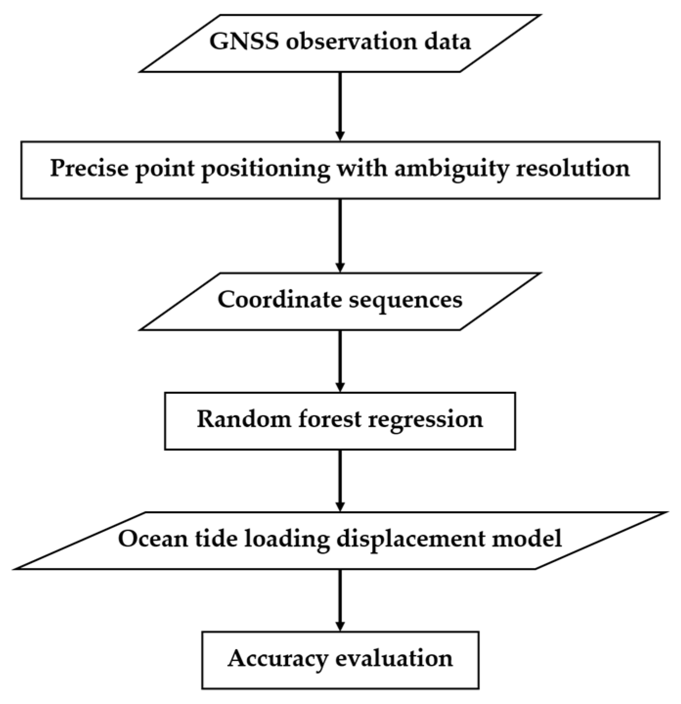
2. Methodology
- Collect short-term GNSS data from multiple stations in a nearby coastal area;
- Perform PPP-AR to obtain high-precision coordinate sequences for the stations;
- Input the coordinate sequences into a random forest regression to fit the empirical model for OTL displacements in the region;
- Evaluate the accuracy of the empirical model.
2.1. Precise Point Positioning
2.2. PPP with Ambiguity Resolution
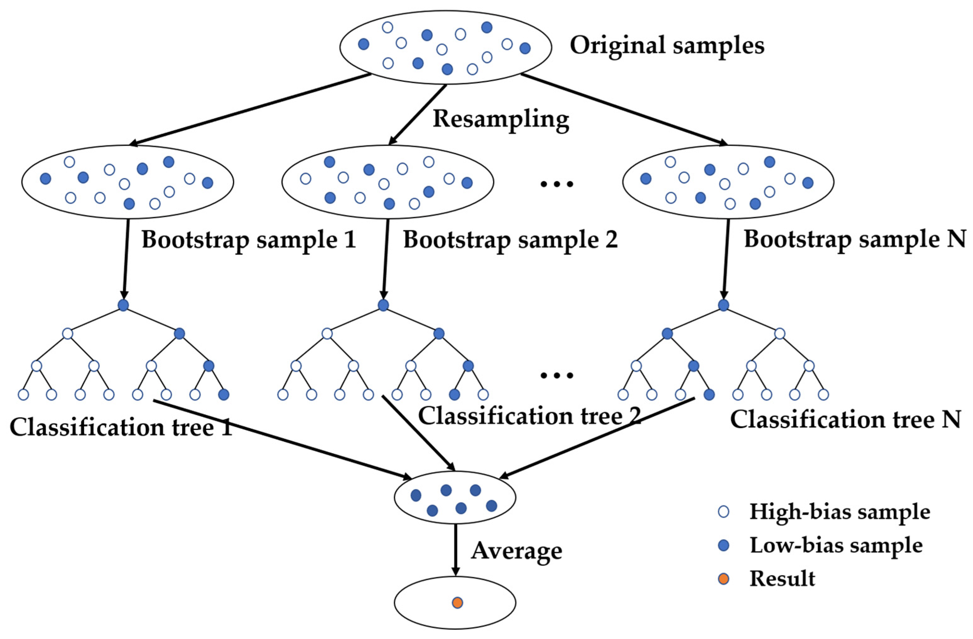
2.3. Random Forest Regression
3. Dataset
4. Model Construction and Evaluation
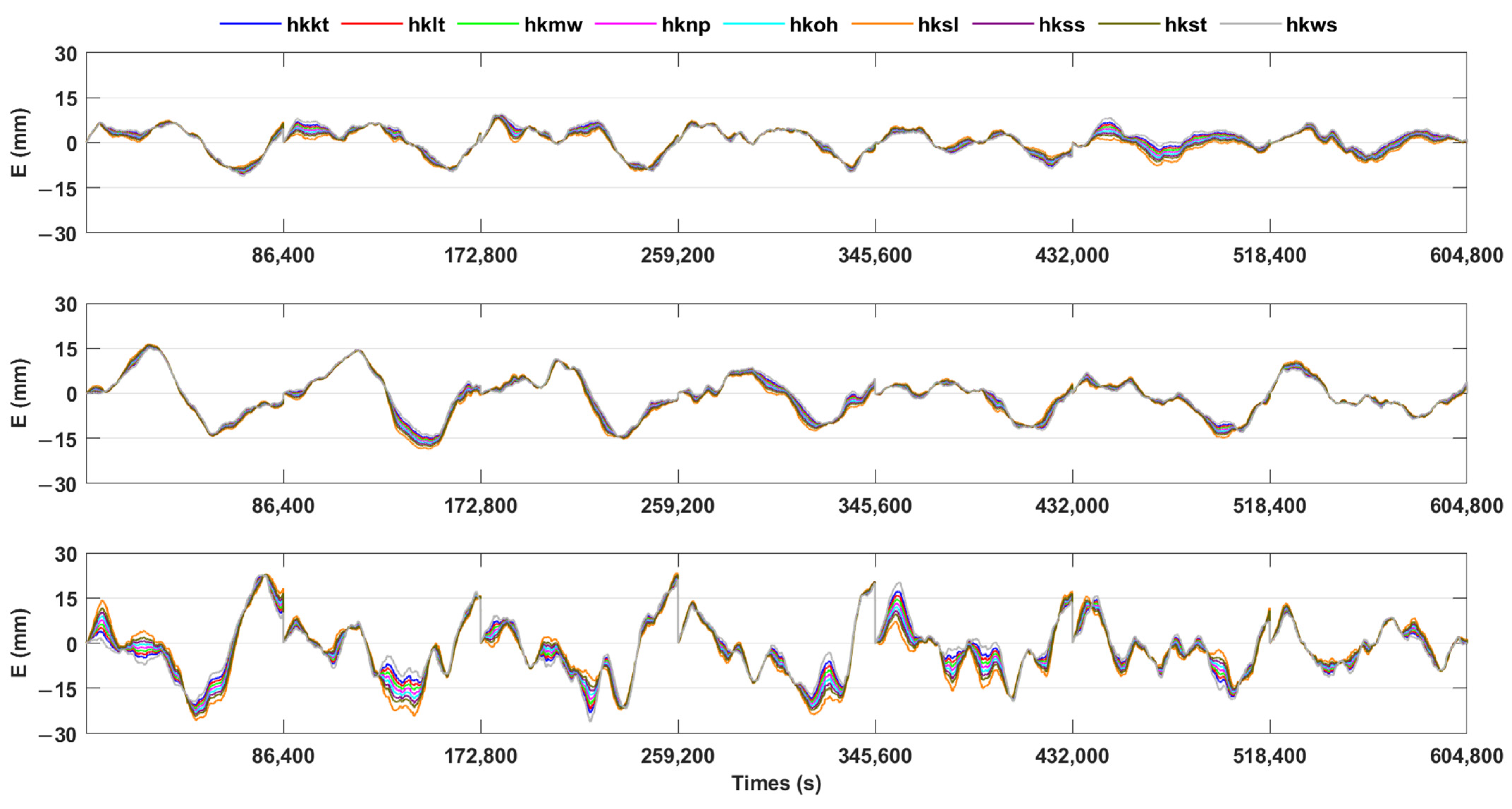
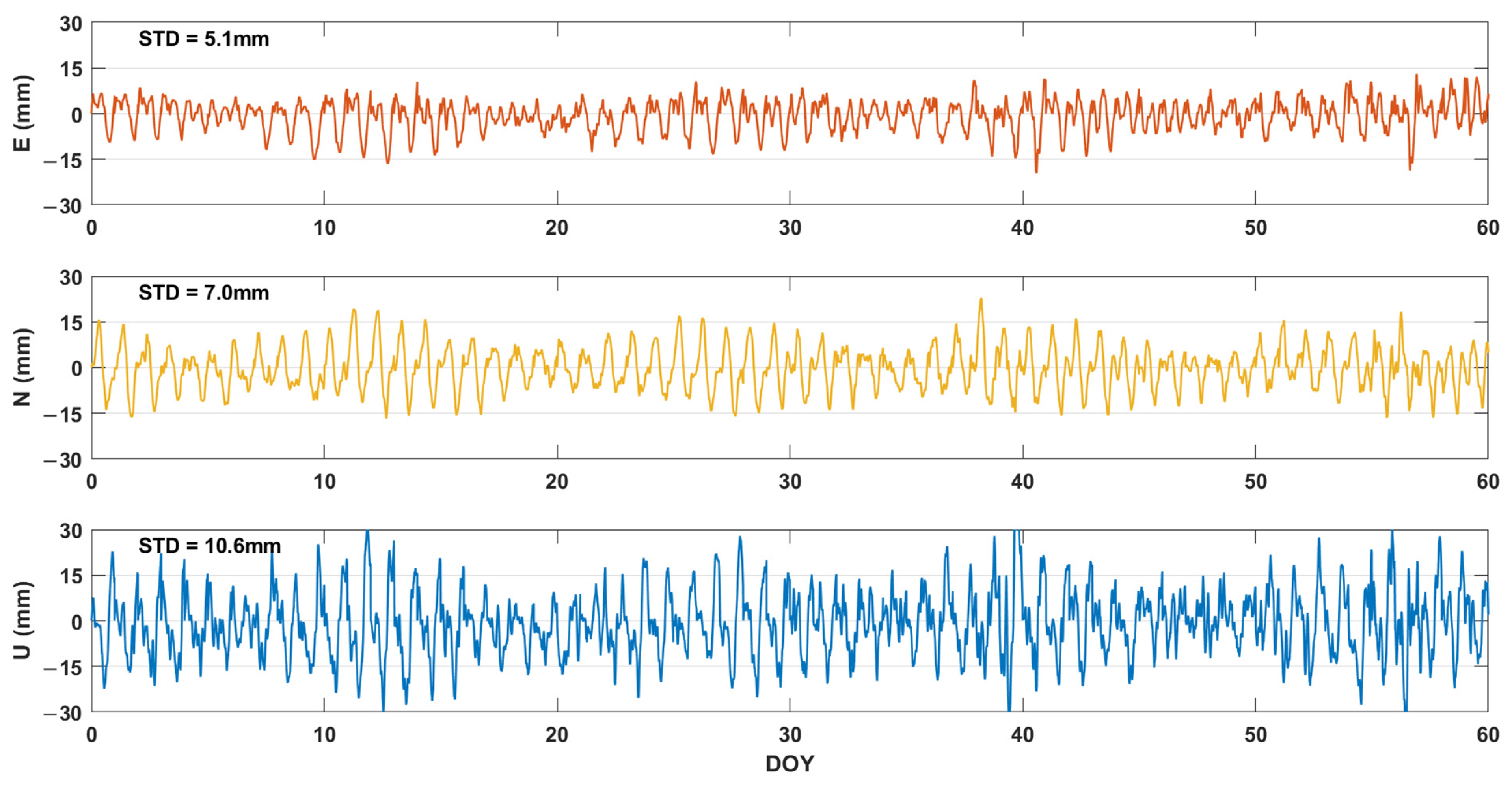
4.1. PPP-AR Solutions
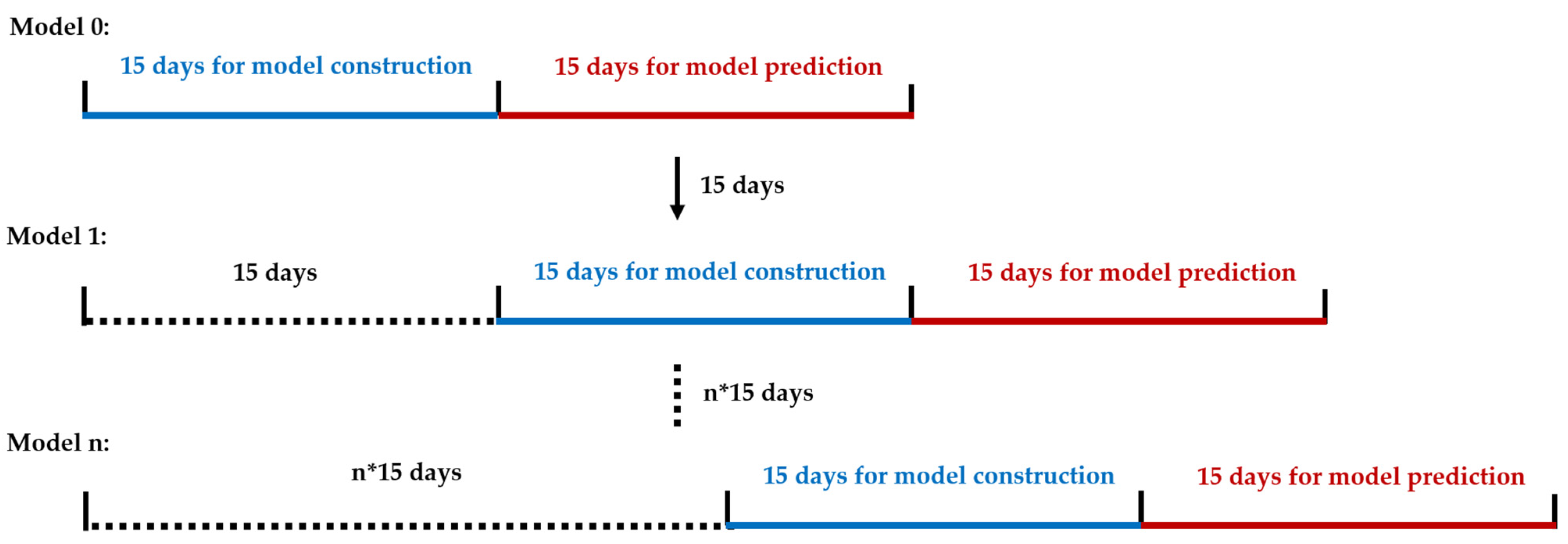
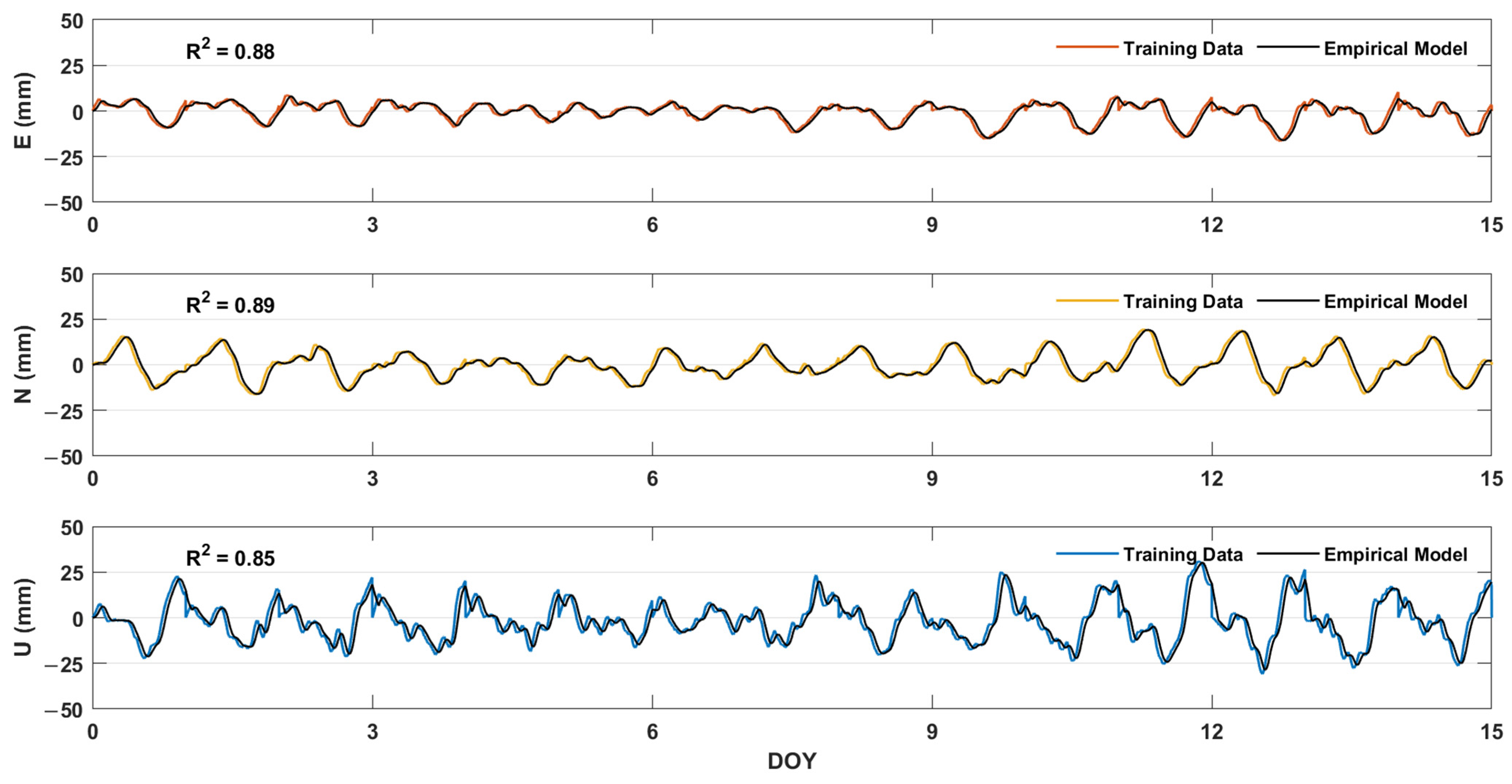
4.2. Model Construction
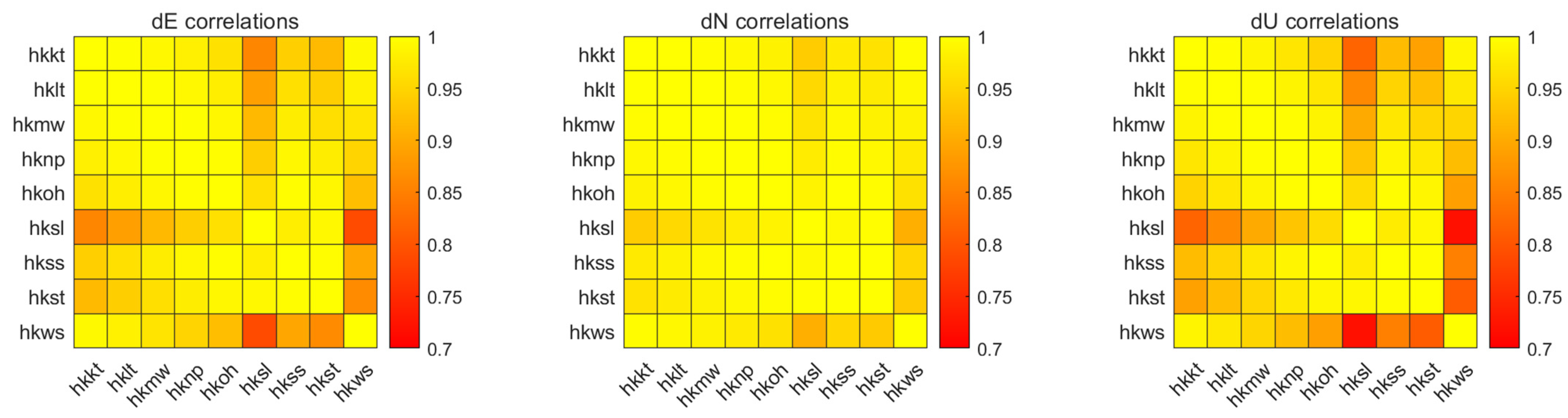
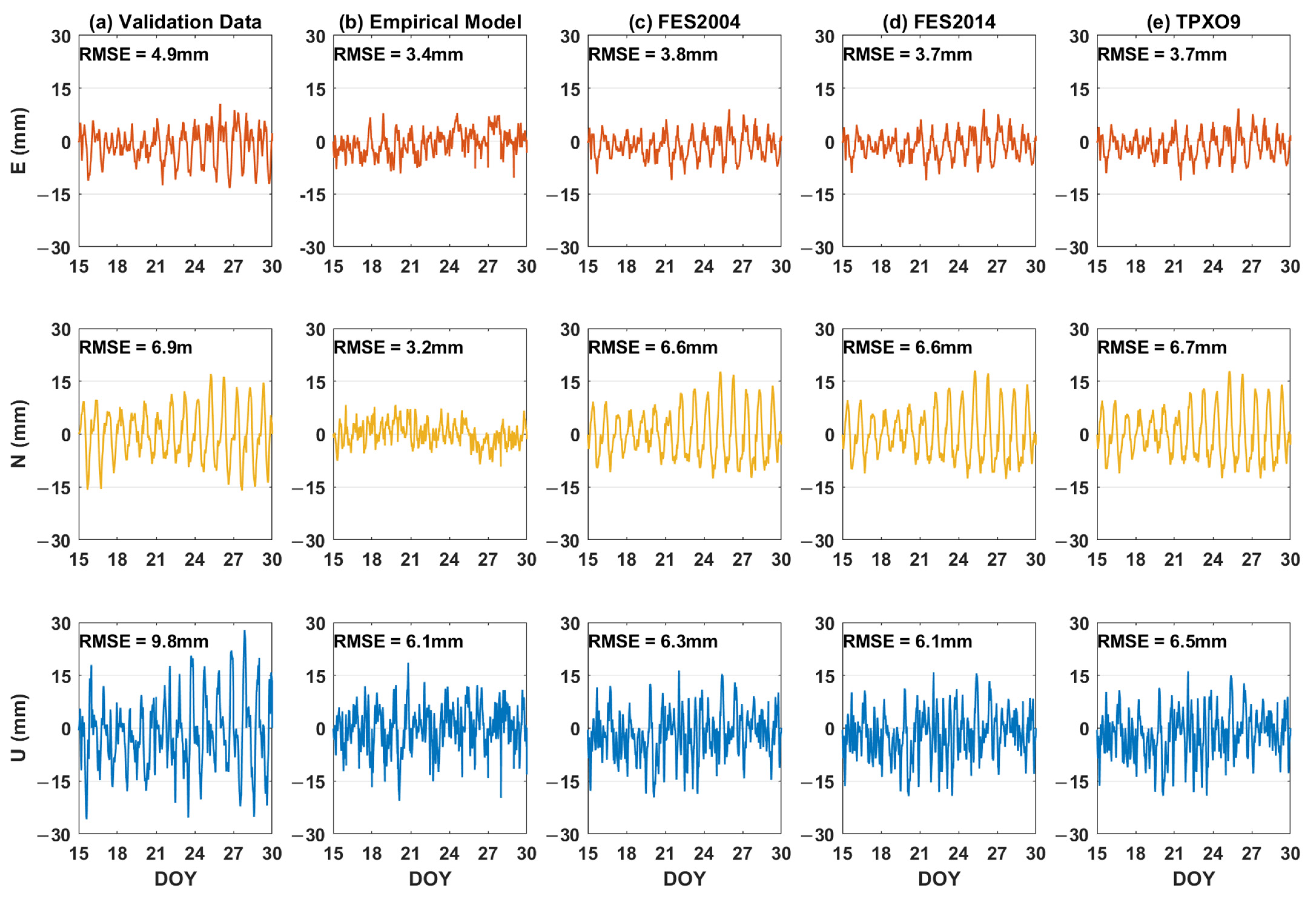
4.3. Accuracy Assessment
5. Discussion
6. Conclusions
Author Contributions
Funding
Data Availability Statement
Acknowledgments
Conflicts of Interest
References
- Jentzsch, G. Earth Tides and Ocean Tidal Loading. In Tidal Phenomena; Springer: Berlin, Germany, 1997; Volume 66, pp. 145–171. [Google Scholar]
- Yuan, L.G.; Ding, X.L.; Zhong, P.; Chen, W.; Huang, D.F. Estimates of ocean tide loading displacements and its impact on position time series in Hong Kong using a dense continuous GPS network. J. Geod. 2009, 83, 999–1015. [Google Scholar] [CrossRef]
- Blewitt, G.; Lavallee, D.; Clarke, P.; Nurutdinov, K. A new global mode of Earth deformation: Seasonal cycle detected. Science 2001, 294, 2342–2345. [Google Scholar] [CrossRef]
- Schwiderski, E.W. On charting global ocean tides. Rev. Geophys. 1980, 18, 243–268. [Google Scholar] [CrossRef]
- Taguchi, E.; Stammer, D.; Zahel, W. Inferring deep ocean tidal energy dissipation from the global high-resolution data-assimilative HAMTIDE model. J. Geophys. Res. Ocean. 2014, 119, 4573–4592. [Google Scholar] [CrossRef]
- Lyard, F.H.; Allain, D.J.; Cancet, M.; Carrère, L.; Picot, N. FES2014 global ocean tide atlas: Design and performance. Ocean Sci. 2021, 17, 615–649. [Google Scholar] [CrossRef]
- Hart-Davis, M.G.; Piccioni, G.; Dettmering, D.; Schwatke, C.; Passaro, M.; Seitz, F. EOT20: A global ocean tide model from multi-mission satellite altimetry. Earth Syst. Sci. Data 2021, 13, 3869–3884. [Google Scholar] [CrossRef]
- Clarke, P.J.; Penna, N.T. Ocean Tide Loading and Relative Gnss in the British Isles. Surv. Rev.-Dir. Overseas Surv. 2010, 42, 212–228. [Google Scholar] [CrossRef]
- Shum, C.K.; Woodworth, P.L.; Andersen, O.B.; Egbert, G.D.; Francis, O.; King, C.; Klosko, S.M.; Le Provost, C.; Li, X.; Molines, J.M.; et al. Accuracy assessment of recent ocean tide model. J. Geophys. Res. Ocean. 1997, 102, 25173–25194. [Google Scholar] [CrossRef]
- Chung, Y.D.; Yeh, T.; Xu, G.; Chen, C.S.; Hwang, C.; Shih, H.C. GPS Height Variations Affected by Ocean Tidal Loading Along the Coast of Taiwan. IEEE Sens. J. 2016, 16, 3697–3704. [Google Scholar] [CrossRef]
- Zumberge, J.F.; Heflin, M.B.; Jefferson, D.C.; Watkins, M.M.; Webb, F.H. Precise point positioning for the efficient and robust analysis of GPS data from large networks. J. Geophys. Res. Solid Earth 1997, 102, 5005–5017. [Google Scholar] [CrossRef]
- King, M.A.; Penna, N.T.; Clarke, P.J.; King, E.C. Validation of ocean tide models around Antarctica using onshore GPS and gravity data. J. Geophys. Res. Solid Earth 2005, 110, 211–235. [Google Scholar] [CrossRef]
- Schenewerk, M.S.; Marshall, J.; Dillinger, W. Vertical Ocean-Loading Deformations Derived from a Global GPS Network. J. Geod. Soc. Jpn. 2001, 47, 237–242. [Google Scholar]
- Allinson, C.R.; Clarke, P.J.; Edwards, S.J.; King, M.A.; Baker, T.F.; Cruddace, P.R. Stability of direct GPS estimates of ocean tide loading. Geophys. Res. Lett. 2004, 31, L15603. [Google Scholar] [CrossRef]
- Urschl, C.; Dach, R.; Hugentobier, U.; Schaer, S.; Beutler, G. Validating ocean tide loading models using GPS. J. Geod. 2005, 78, 616–625. [Google Scholar] [CrossRef]
- Wang, H.; Li, M.; Wei, N.; Han, S.; Zhao, Q. Improved estimation of ocean tide loading displacements using multi-GNSS kinematic and static precise point positioning. GPS Solut. 2024, 28, 27. [Google Scholar] [CrossRef]
- Ito, T.; Okubo, M.; Sagiya, T. High resolution mapping of Earth tide response based on GPS data in Japan. J. Geodyn. 2009, 48, 253–259. [Google Scholar] [CrossRef]
- Khan, S.A.; Tscheming, C.C. Determination of semi-diurnal ocean tide loading constituents using GPS in Alaska. Geophys. Res. Lett. 2001, 28, 2249–2252. [Google Scholar] [CrossRef]
- King, M. Kinematic and static GPS techniques for estimating tidal displacements with application to Antarctica. J. Geodyn. 2006, 41, 77–86. [Google Scholar] [CrossRef]
- Bos, M.S.; Penna, N.T.; Baker, T.F.; Clarke, P.J. Ocean tide loading displacements in western Europe: 2. GPS-observed anelastic dispersion in the asthenosphere. J. Geophys. Res. Solid Earth 2015, 120, 6540–6557. [Google Scholar] [CrossRef]
- Abbaszadeh, M.; Clarke, P.J.; Penna, N.T. Benefits of combining GPS and GLONASS for measuring ocean tide loading displacement. J. Geod. 2020, 94, 63. [Google Scholar] [CrossRef]
- Peng, W.; Wang, Q.; Cao, Y.; Xing, X.; Hu, W. Evaluation of Tidal Effect in Long-Strip DInSAR Measurements Based on GPS Network and Tidal Models. Remote Sens. 2022, 14, 2954. [Google Scholar] [CrossRef]
- Matviichuk, B.; King, M.; Watson, C.; Bos, M. Comparison of state-of-the-art GNSS-observed and predicted ocean tide loading displacements across Australia. J. Geod. 2023, 97, 78. [Google Scholar] [CrossRef]
- Geng, J.; Meng, X.; Dodson, A.H.; Teferle, F.N. Integer ambiguity resolution in precise point positioning: Method comparison. J. Geod. 2010, 84, 569–581. [Google Scholar] [CrossRef]
- Laurichesse, D.; Mercier, F.; Berthias, J.P.; Broca, P.; Cerri, L. Integer Ambiguity Resolution on Undifferenced GPS Phase Measurements and Its Application to PPP and Satellite Precise Orbit Determination. Navigation 2009, 56, 135–149. [Google Scholar] [CrossRef]
- Collins, P.; Bisnath, S.; Lahaye, F.; Héroux, P. Undifferenced GPS Ambiguity Resolution Using the Decoupled Clock Model and Ambiguity Datum Fixing. Navigation 2010, 57, 123–135. [Google Scholar] [CrossRef]
- Ge, M.; Gendt, G.; Rothacher, M.; Shi, C.; Liu, J. Resolution of GPS carrier-phase ambiguities in Precise Point Positioning (PPP) with daily observations. J. Geod. 2008, 82, 389–399. [Google Scholar] [CrossRef]
- Geng, J.; Chen, X.; Pan, Y.; Zhao, Q. A modified phase clock/bias model to improve PPP ambiguity resolution at Wuhan University. J. Geod. 2019, 93, 2053–2067. [Google Scholar] [CrossRef]
- Geng, J.; Chen, X.; Pan, Y.; Mao, S.; Li, C.; Zhou, J.; Zhang, K. PRIDE PPP-AR: An open-source software for GPS PPP ambiguity resolution. GPS Solut. 2019, 23, 91. [Google Scholar] [CrossRef]
- Breiman, L. Random Forests. Mach. Learn. 2001, 45, 5–32. [Google Scholar] [CrossRef]
- Strobl, C.; Boulesteix, A.; Kneib, T.; Augustin, T.; Zeileis, A. Conditional variable importance for random forests. BMC Bioinform. 2008, 9, 307. [Google Scholar] [CrossRef]
- Yuan, L.; Chao, B.F.; Ding, X.; Zhong, P. The tidal displacement field at Earth’s surface determined using global GPS observations. J. Geophys. Res. Solid Earth 2013, 118, 2618–2632. [Google Scholar] [CrossRef]
- Penna, N.T.; Bos, M.S.; Baker, T.F.; Scherneck, H.G. Assessing the accuracy of predicted ocean tide loading displacement values. J. Geod. 2008, 82, 893–907. [Google Scholar] [CrossRef]
- Melbourne, W. The case for ranging in GPS-based geodetic systems. In Proceedings of the First International Symposium on Precise Positioning with the Global Positioning System, Rockville, MD, USA, 15–19 April 1985; pp. 373–386. [Google Scholar]
- Wübbena, G. Software developments for geodetic positioning with GPS using TI-4100 code and carrier measurements. In Proceedings of the First International Symposium on Precise Positioning with the Global Positioning System, Rockville, MD, USA, 15–19 April 1985; pp. 403–412. [Google Scholar]
- TEUNISSEN, P.J.G. The least-squares ambiguity decorrelation adjustment: A method for fast GPS integer ambiguity estimation. J. Geod. 1995, 70, 65–82. [Google Scholar] [CrossRef]
- Zhou, M.; Liu, X.; Guo, J.; Jin, X.; Chang, X. Ocean Tide Loading Displacement Parameters Estimated From GNSS-Derived Coordinate Time Series Considering the Effect of Mass Loading in Hong Kong. IEEE J. Sel. Top. Appl. Earth Observ. Remote Sens. 2020, 13, 6064–6076. [Google Scholar] [CrossRef]
- Guo, J.; Xu, X.; Zhao, Q.; Liu, J. Precise orbit determination for quad-constellation satellites at Wuhan University: Strategy, result validation, and comparison. J. Geod. 2016, 90, 143–159. [Google Scholar] [CrossRef]
- Rebischung, P.; Schmid, R. IGS14/igs14.atx: A new framework for the IGS products. In Proceedings of the AGU Fall Meeting 2016, San Francisco, CA, USA, 12–16 December 2016. [Google Scholar]
- Saastamoinen, J. Atmospheric Correction for the Troposphere and Stratosphere in Radio Ranging Satellites. In Geophysical Monograph Series; American Geophysical Union: Washington, DC, USA, 1972; Volume 15, pp. 247–251. [Google Scholar]
- Petit, G.; Luzum, B. IERS Conventions (2010); International Earth Rotation and Reference Systems Service: Frankfurt am Main, Germany, 2010. [Google Scholar]
- Zhou, M.; Liu, X.; Yuan, J.; Jin, X.; Niu, Y.; Guo, J.; Gao, H. Seasonal Variation of GPS-Derived the Principal Ocean Tidal Constituents’ Loading Displacement Parameters Based on Moving Harmonic Analysis in Hong Kong. Remote Sens. 2021, 13, 279. [Google Scholar] [CrossRef]
- Pawlowicz, R.; Beardsley, B.; Lentz, S. Classical tidal harmonic analysis including error estimates in MATLAB using T_TIDE. Comput. Geosci. 2002, 28, 929–937. [Google Scholar] [CrossRef]
- Pan, H.; Lv, X.; Wang, Y.; Matte, P.; Chen, H.; Jin, G. Exploration of Tidal-Fluvial Interaction in the Columbia River Estuary Using S_TIDE. J. Geophys. Res. Ocean. 2018, 123, 6598–6619. [Google Scholar] [CrossRef]
- Godin, G. The Analysis of Tides; University of Toronto Press: Toronto, ON, Canada, 1972. [Google Scholar]


| Parameters | Processing Strategies |
|---|---|
| Satellite system | GPS: L1/L2; Galileo: E1/E5a; GLONASS: R1/R2 |
| Interval | 30 s |
| Weighting | Elevation-dependent data weighting |
| Observation cut-off | 10° |
| Satellite orbits | SP3 products by Wuhan University [38] |
| Satellite clocks | CLK products by Wuhan University [38] |
| ERP parameters | ERP products by Wuhan University [38] |
| Undifferenced ambiguity resolution | BIA products by Wuhan University [28] Ambiguity fixing for the GPS and Galileo Float solution for the GLONASS |
| PCV and PCO | ATX files by IGS [39] |
| Ionospheric delay | Iono-Free LC |
| Tropospheric delay | Saastamoinen model [40] |
| Reference frame | IGS14 |
| Geocenter motion | IERS Conventions 2010 [41] |
| Solid Earth tides and pole tides | IERS Conventions 2010 |
| Training Data | Validation Data | RMSE (mm) | ||
|---|---|---|---|---|
| East | North | Up | ||
| DOY 001-015 | DOY 016-030 | 3.4 | 3.2 | 6.1 |
| DOY 031-045 | 3.8 | 3.9 | 7.4 | |
| DOY 046-060 | 5.1 | 5.0 | 8.5 | |
| DOY 016-030 | DOY 031-045 | 3.4 | 3.2 | 6.1 |
| DOY 046-060 | 4.0 | 4.3 | 7.5 | |
| DOY 031-045 | DOY 046-060 | 3.8 | 3.8 | 6.9 |
| Direction | Tidal Constituent | Empirical Model | FES2014 | ||
|---|---|---|---|---|---|
| Amplitude (mm) | Phase (°) | Amplitude (mm) | Phase (°) | ||
| East | M2 | 3.56 | 127.7 | 2.23 | 129.5 |
| S2 | 1.08 | 137.2 | 1.00 | 137.0 | |
| K1 | 2.22 | −86.9 | 1.69 | −76.1 | |
| O1 | 1.43 | −98.6 | 1.36 | −98.8 | |
| North | M2 | 4.03 | 139.3 | 1.47 | 23.6 |
| S2 | 1.49 | −70.4 | 0.52 | 58.1 | |
| K1 | 8.47 | −79.8 | 2.58 | 177.7 | |
| O1 | 2.49 | 149.1 | 2.22 | 142.3 | |
| Up | M2 | 6.03 | −167.5 | 6.80 | −167.9 |
| S2 | 2.28 | −150.1 | 1.78 | −145.1 | |
| K1 | 6.52 | −16.5 | 6.78 | −17.3 | |
| O1 | 6. 95 | −44.8 | 7.32 | −49.6 | |
Disclaimer/Publisher’s Note: The statements, opinions and data contained in all publications are solely those of the individual author(s) and contributor(s) and not of MDPI and/or the editor(s). MDPI and/or the editor(s) disclaim responsibility for any injury to people or property resulting from any ideas, methods, instructions or products referred to in the content. |
© 2024 by the authors. Licensee MDPI, Basel, Switzerland. This article is an open access article distributed under the terms and conditions of the Creative Commons Attribution (CC BY) license (https://creativecommons.org/licenses/by/4.0/).
Share and Cite
Wang, H.; Yan, X.; Yang, M.; Feng, W.; Zhong, M. A Method for Constructing an Empirical Model of Short-Term Offshore Ocean Tide Loading Displacement Based on PPP. Remote Sens. 2024, 16, 2998. https://doi.org/10.3390/rs16162998
Wang H, Yan X, Yang M, Feng W, Zhong M. A Method for Constructing an Empirical Model of Short-Term Offshore Ocean Tide Loading Displacement Based on PPP. Remote Sensing. 2024; 16(16):2998. https://doi.org/10.3390/rs16162998
Chicago/Turabian StyleWang, Hai, Xingyuan Yan, Meng Yang, Wei Feng, and Min Zhong. 2024. "A Method for Constructing an Empirical Model of Short-Term Offshore Ocean Tide Loading Displacement Based on PPP" Remote Sensing 16, no. 16: 2998. https://doi.org/10.3390/rs16162998
APA StyleWang, H., Yan, X., Yang, M., Feng, W., & Zhong, M. (2024). A Method for Constructing an Empirical Model of Short-Term Offshore Ocean Tide Loading Displacement Based on PPP. Remote Sensing, 16(16), 2998. https://doi.org/10.3390/rs16162998