Article

A Framework for Subregion Ensemble Learning Mapping of Land Use/Land Cover at the Watershed Scale

1
Key Laboratory of Tibetan Plateau Land Surface Processes and Ecological Conservation (Ministry of Education), Qinghai Normal University, Xining 810008, China
2
Qinghai Provincial Key Laboratory of Physical Geography and Environmental Process, College of Geographical Science, Qinghai Normal University, Xining 810008, China
3
Academy of Plateau Science and Sustainability, People’s Government of Qinghai Province & Beijing Normal University, Xining 810008, China
*
Author to whom correspondence should be addressed.
Remote Sens. 2024, 16(20), 3855; https://doi.org/10.3390/rs16203855
Submission received: 27 August 2024 / Revised: 6 October 2024 / Accepted: 14 October 2024 / Published: 17 October 2024
(This article belongs to the Special Issue Monitoring Cold-Region Water Cycles Using Remote Sensing Big Data)

Abstract

:
Land use/land cover (LULC) data are essential for Earth science research. Due to the high fragmentation and heterogeneity of landscapes, machine learning-based LULC classification frequently emphasizes results such as classification accuracy, efficiency, and variable importance analysis. However, this approach often overlooks the intermediate processes, and LULC mapping that relies on a single classifier typically does not yield satisfactory results. In this paper, to obtain refined LULC classification products at the watershed scale and improve the accuracy and efficiency of watershed-scale mapping, we propose a subregion ensemble learning classification framework. The Huangshui River watershed, located in the transition belts between the Qinghai-Tibet Plateau and Loess Plateau, is chosen as the case study area, and Sentinel-2A/B multi-temporal data are selected for ensemble learning classification. Using the proposed method, the block classification scale is analyzed and illustrated at the watershed, and the classification accuracy and efficiency of the new method are compared and analyzed against three ensemble learning methods using several variables. The proposed watershed-scale ensemble learning framework has better accuracy and efficiency for LULC mapping and has certain advantages over the other methods. The method proposed in this study provides new ideas for watershed-scale LULC mapping technology.

Graphical Abstract

1. Introduction

Land use/land cover (LULC) is a comprehensive product, constituting an important type of data for understanding the relationship between human activities and the environment [1]. Land cover refers to the complex natural features and artificial creations on the Earth’s surface, such as vegetation, water, soil, and construction land, while land use refers to human-induced land change activities [2]. LULC data have been used in many research fields, such as food security, climate change, homeland spatial planning, disaster risk assessment, and global change [3,4], meaning the accuracy of LULC data impacts a wide range of studies [5]. LULC mapping includes traditional field survey mapping and remote sensing image mapping. Field survey mapping is a direct mapping method, which is time-consuming and labor-intensive as it requires determining LULC over large areas manually and inevitably entails a certain degree of subjectivity. LULC mapping based on remotely sensed imagery has the advantages of low cost, high efficiency, and fast timeliness [6].
Remote sensing image mapping is one of the most important applications for extracting thematic information from remotely sensed data, which refers to the extraction of specific content from spatial features by applying certain classification algorithms. Such algorithms can be used to determine the accuracy of LULC types to some extent. Many different methods have been applied in multispectral image classification, such as supervised and unsupervised classification, parametric and nonparametric, semantic segmentation, and other classifications. The most widely applied methods are unsupervised and supervised learning. The initial classification methods in supervised learning are the minimum distance method, maximum likelihood method, and multilevel segmentation method. With the development of statistical learning theory methods, artificial intelligence (AI), and big data, machine learning methods have attracted increasing attention in LULC mapping in recent years [7,8]. Decision tree (DT), support vector machine (SVM), artificial neural networks (ANN), naive bayes (NB), random forest (RF), etc., have become the most popular machine learning methods. In the last decade, various machine learning algorithms have been extensively applied for LULC classification [9,10,11], such as SVM and RF, which yield higher accuracy than traditional classification [12].
The classification of remotely sensed images is a complex process that may be affected by many factors. One of the main causes of classification errors is that a single classifier may be unable to distinguish between different classes. To reduce classification errors, an effective solution is to generate ensemble classifiers by combining single classifiers with complementary advantages, also known as ensemble learning classification. Ensemble classification includes the integration of homogeneous and heterogeneous classifiers using certain combination methods. In ensemble learning, a homogeneous classifier ensemble uses the same type of models (such as multiple decision trees) to improve stability and accuracy, typically implemented through Bagging or Boosting methods. In contrast, a heterogeneous classifier ensemble combines different types of models (such as DT, SVM, etc.) to leverage their respective strengths and enhance overall performance, with common methods including Stacking and Voting. Due to the great potential shown by ensemble learning in improving the accuracy and reliability of classification, ensemble learning has been preliminarily applied to the classification of LULC in recent years, and related studies have shown that bagging, boosting, and stacking integration result in higher accuracy and greater classification efficiency compared with traditional classification methods [13]. Though the principles, strengths, and weaknesses of each single classifier in ensemble classification are different, they are often complementary for classification tasks; as such, ensemble learning classification has been gradually applied in LULC studies by many researchers [14,15].
RF is a typical representative of bagging integration which has been applied to LULC classification in recent years [16]. Chan et al. [17] showed that RF with bootstrap self-sampling in LULC classification produces overfitting, and the subsequent random selectivity is difficult to explain. Differing from the bagging integration method, boosting requires the integration of trees in the classifier based on the weighted distribution of training samples, which changes the random selection of trees in RF and has the advantage of paying more attention to samples misclassified in the previous round. Typical representatives of boosting integration methods are gradient boosting decision tree (GBDT), extreme gradient boosting (XGBoost), light gradient boosting machine (LightGBM), and other algorithms. Yang et al. [18] utilized multisource remote sensing data and created an object-oriented approach by combining GBDT, RF, and SVM to extract LULC-type data, and their results showed that GBDT has higher accuracy than RF. Abdullah et al. [19] applied the XGBoost algorithm to long time series remote sensing product mapping and showed that it can effectively solve spectral complexity and landscape heterogeneity and has certain advantages for long time series remote sensing mapping. Wen et al. [14] utilized the bagging, boosting, and stacking algorithms in ensemble methods to extract coastal wetlands. Their results indicated that the ensemble classifiers have certain superiority for accurate wetland localization.
Among current methods, LightGBM, a distributed gradient boosting algorithm, has better accuracy than RF, GBDT, and XGBoost in prediction, but it is rarely applied in classification [20]. From previous related studies, the ensemble classification method has been shown to have higher classification accuracy and efficiency and has great potential for application in LULC classification. Next, stacking is a strategy for integrating heterogeneous types of base classifiers for ensemble learning and classification. Stacking ensemble learning uses the original training samples to train a first-level learner and then uses the output of the first-level learner as the input features and the corresponding original tokens as new tokens to compose a new dataset to train a second-level learner and output the final classification result. The stacking integration method can complement the advantages of different classifiers and their results are better than those obtained with a single classifier, making them worth exploring for LULC classification [21].
Currently, published land use products generally have low update frequencies, typically released based on benchmark years such as 2010, 2015, and 2020 [22]. The data quality is uneven, with differences in accuracy, resolution, and coverage among various sources. Some data cannot be downloaded for free, which limits their widespread use. Through actual surveys and comparisons, the publicly available land use and land cover products in the Huangshui River basin are generally of average quality, with considerable variations in detail. While the data perform well in mountainous areas, accurately reflecting the true land cover, there are significant discrepancies in urban areas and around cities and counties [23,24]. Besides this, LULC mapping on a global scale is generally based on the principle of regional to global due to the limitations of computational resources and the large amount of data in the parameter datasets used for mapping [25]. For the remote sensing classification of LULC at the national, intercontinental, and global scales, or related classification studies based on the Google Earth Engine (GEE) cloud platform or Pixel Image Engine, the usual approach is to first chunk/subsection the whole study area and then classify each chunk/subsection. In this approach, the classification results of each chunk/subsection are stitched together and the accuracy of the classification mapping is averaged over the whole study area. At these scales, it is reasonable and feasible to adopt the method of classifying each subsection individually for LULC classification. At smaller scales, such as watersheds (which are a microcosm of the Earth system, possessing similar complexity to the entire land surface system and a high degree of fragmentation and heterogeneity), classifications can be limited by edge effects, resulting in large classification errors if chunks/subplots are used for training in the model classification process, as each subplot requires its own model. Although the same classifier is used, due to the different optimal parameters obtained by each classifier, such as the different internal structures of the RF algorithm, the leaf nodes of the tree and the depth of the tree will be different. These, coupled with errors caused by edge effects, mean the classification accuracy of the individual chunks can often be low, resulting in inaccurate classification results at the watershed scale.
Therefore, the aim of this study is to investigate and develop a watershed-scale LULC mapping framework based on subregion ensemble learning in order to improve the efficiency, accuracy, and spatial consistency of LULC mapping. To this aim, we selected the Huangshui River watershed in the upper reaches of the Yellow River as our study region and compared the classification results obtained with three ensemble learning algorithms: RF, improved LightGBM, and stacking. Our specific research objectives are (1) to compare and analyze the block classification on the basin scale, (2) to compare and analyze the cartographic effects of the three ensemble models, and (3) to provide a suitable LULC mapping framework for watershed-scale studies.

2. Study Area and Data Preprocessing

2.1. Overview of the Study Area

Huangshui Basin, located in the northeast region of Qinghai Province, is the northeast basin of the Qinghai–Tibetan Plateau, situated geographically from 36°02′ to 37°28′N, 100°42′ to 103°04′E, with a total area of 16,120 km2 and an elevation range of 1650 m to 4860 m a.s.l. The Huangshui River is the largest first-level tributary upstream of the Yellow River, and the watershed includes several administrative areas including Xining City, Datong County, Huangyuan County, Huangzhong District, Haiyan County, Huzhu County, Ping’an District, Ledu District, and Minhe County. Huangshui Basin is the main population gathering area of Qinghai Province and features a large diversity of LULC changes caused by human activities. Xining City is the capital city of Qinghai Province, which is the political, economic, transportation, and cultural center of Qinghai Province, and Haidong City is located to the east of Xining City. The topography of the study area consists of undulating, diverse landforms, hills, and mid-altitude mountainous terrain.
Huangshui Basin in Qinghai Province is separated from the Yellow River Basin to the south by the Laji Mountains, to the north by the Daban Mountains and the Datong River Basin, and to the east by the Riyue Mountains on the shores of Qinghai Lake. It has an arid and semi-arid continental climate, with an average annual precipitation of 300–500 mm, and is an important agricultural area on the Qinghai–Tibetan Plateau [26]. As a natural geographic unit of the Qinghai–Tibetan Plateau, the topography and climate of Huangshui Basin jointly influence the natural geographic environment, endowing it with a large variety of soil, vegetation, and landscape characteristics, making it a particularly unique watershed. Therefore taking Huangshui Basin as a typical representative of the Qinghai–Tibetan Plateau, the objective of the study is to explore and quantify LULC classification in the basin, providing guidance for future planning and management and giving certain practical significance for other similar terrain. The location of the study area is shown in Figure 1.

2.2. Data Sources

The data used in this paper are Sentinel-2A/B images freely available on the GEE platform, which have been processed into a surface reflectance product that can be used directly [27,28]. Generally, LULC data obtained in recent years can reflect the latest distribution of all kinds of features in a certain region, while multi-seasonal data obtained throughout the year can reflect the response of vegetation to season. In this paper, we study seasonal images obtained in 2021. Due to its location, the climate on the Tibetan Plateau is cold, and from December to April, parts of the ground and mountains are covered in snow, making LULC monitoring unfavorable. As such, we excluded data from these months in our study and only consider images from May to November. Next, due to the influence of clouds, some images obtained during May to November contain high amounts of cloud cover. In addition, coupled with the large area of the watershed, at least three months of imagery were needed, which were stitched together to form an image that is applicable to the entire watershed for the purpose of LULC categorization. In view of the above factors, and taking into account the various climatic factors and seasonal vegetation phenology in the study area, we employed images from the spring/summer months of April to August in 2021, which reflect the greening, growing, and maturing periods of plants. We also synthesized a three-month image (September–November 2021) as a winter image to reflect the wilting and fading periods of plants.
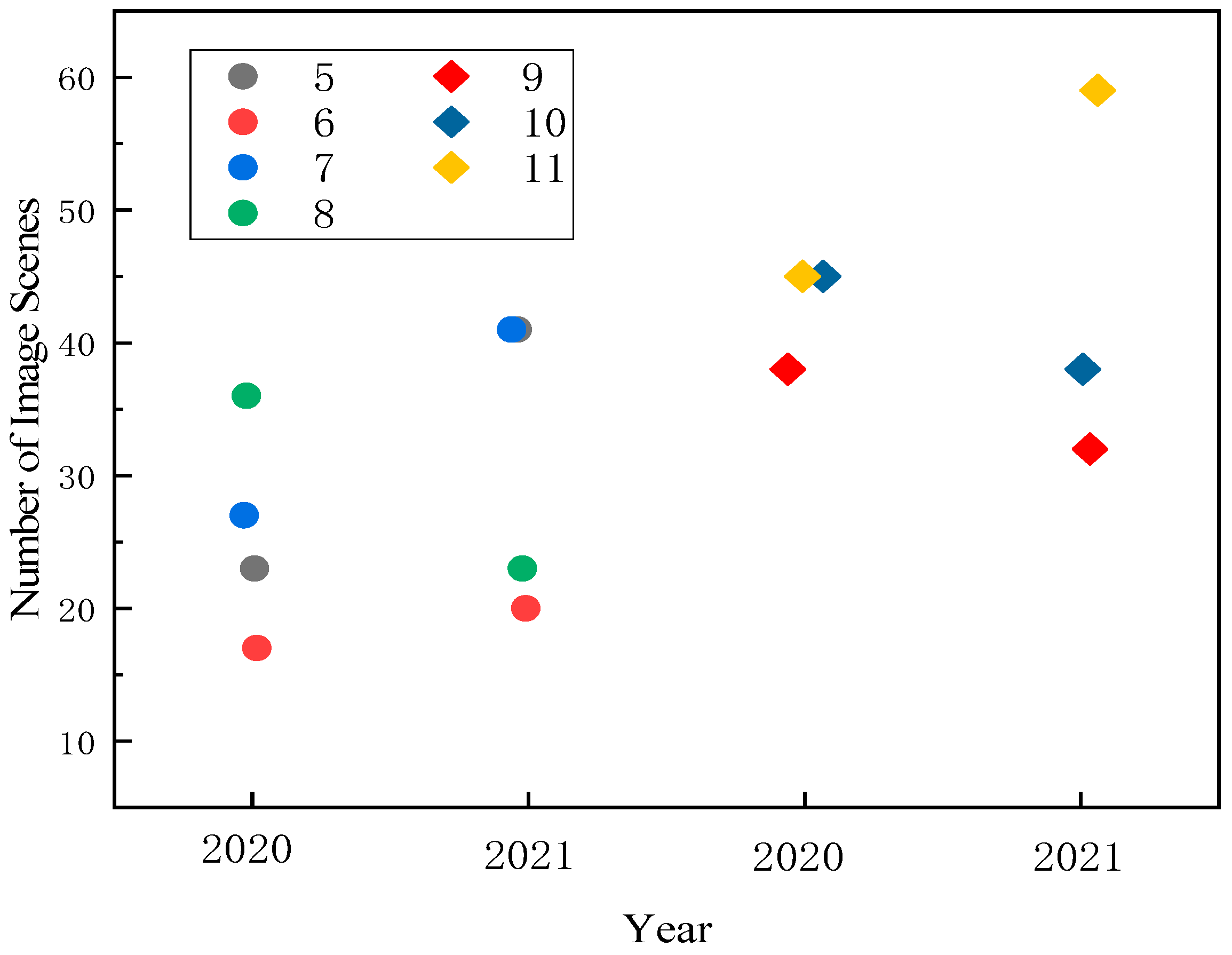
Our code was written in GEE to synthesize the winter and summer images. Since the synthesized images contain some mountainous areas covered by clouds, all null values produced after de-clouding were filled in using data of the same area and day/month from 2020; this method is deemed suitable due to the very similar surface cover conditions present in both 2020 and 2021. The applied image statistics are shown in Figure 2. Due to the topography of the watershed leading to relatively fragmented areas, spatial resolution is important. Therefore, the blue, green, red, and near-infrared bands (with a resolution of 10 m) were chosen as the spectral bands used for each period in the study. In addition to the original spectral bands, we also used datasets of four feature parameters: primary band, spectral index features, textural features, and topographic features. Among them, the original bands are the co-added summer and winter images, with a total of 8 bands, three spectral indices, with a total of 6 bands, eight textural features, with a total of 16 bands, and three topographic features, with a total of 33 bands, constituting the feature dataset classified in this paper, as shown in Table 1 [29,30,31,32,33,34,35,36,37,38,39,40,41].

2.3. Classification System

A prerequisite and foundation of LULC classification is first to determine the LULC classification system, which should take into account the actual situation of the study area and the data sources and should be based on an existing classification system. At present, the “National Remote Sensing Monitoring LULC Classification System” gives six primary categories and six secondary categories, based on actual field research and the spatial resolution of the Sentinel-2A/B data: cropland; forested land; shrubland; open forest land; other forested land; high-cover grassland; medium-cover grassland; low-cover grassland; rivers, reservoirs, and ponds; unutilized land; and permanent snow on land.

3. Research Methodology

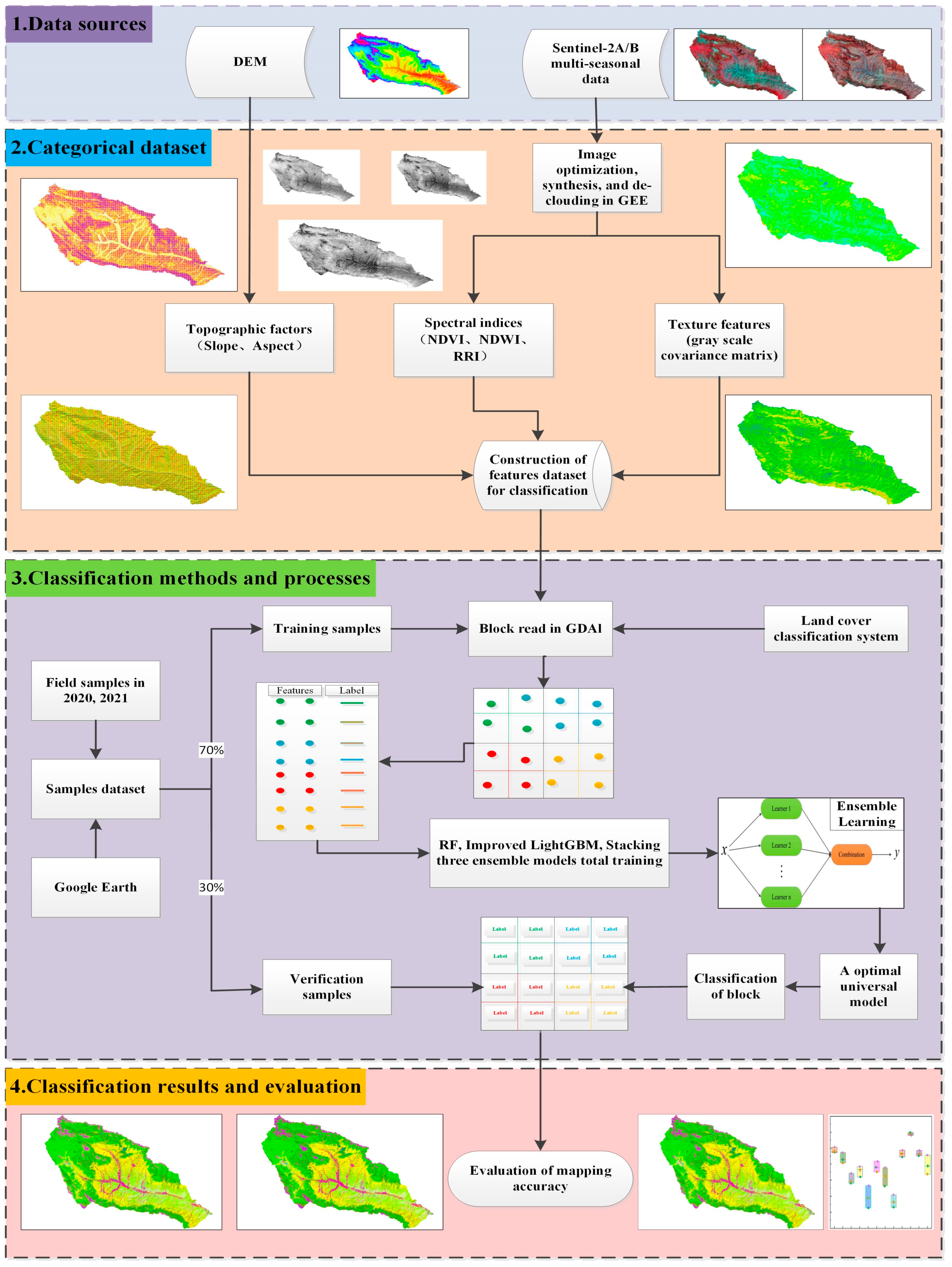
The flowchart in Figure 3 shows the ensemble learning mapping framework used in this study. The main steps include data sourcing, creation of the feature dataset, the mapping method and process, and result evaluation. The following sections describe the analysis scheme and several relevant steps of this framework in detail.

3.1. Random Forest

RF is an ensemble learning method that performs classification and regression tasks by constructing multiple decision trees. It is the most representative bagging integration learning algorithm, and the combination of bagging integrative learning and stochastic subspace methods is beneficial to preventing overfitting [42]. When selecting the segmentation point in each decision tree, RF randomly selects a feature subset and then performs random segmentation selection on the dataset. In the classification process, a dataset with different subsamples is randomly selected, and a number of decision trees are trained using different feature subsamples. The results of the subsample decision trees are voted on, and the final classification results are outputted. RF has become the most widely used machine learning algorithm due to the fact that it combines the advantages of multiple decision trees with high accuracy, has strong resistance to overfitting, handles large-scale data very well, and has strong interpretability.

3.2. Improved LightGBM

LightGBM is a type of boosting integration scheme, consisting of a distributed gradient boosting algorithm based on decision trees [43,44]. Because of its lower computational efficiency and large memory consumption, it is difficult for the bagging algorithm to compute large sets of data. To solve these problems, LightGBM uses the gradient-based one-side sampling (GOSS) and exclusive feature bundling (EFB) methods for gradients. The GOSS method reduces a large amount of data with only small gradients by computing the information gain via the use of training samples. In this approach, only sample points with large gradients are retained while training samples with small gradients are removed; this method yields more accurate results than obtained with just random sampling. Generally speaking, when extracting LULC types from remote sensing images, the gradient at the edge of a feature type is larger, while the gradient inside the feature is smaller and more homogeneous. The EFB method is more advantageous for big data computations, mainly because of the bundling and dimensionality reduction of the considered features. In addition, LightGBM uses histograms for differential optimization, which reduce the consumption of memory and improve the computational efficiency. Currently, LightGBM has mainly been used in research related to predictions [45,46]. The main process of LightGBM computation is described in the following.
In training, LightGBM calculates the corresponding loss function L ( y , F t 1 ( x ) ) according to the learner, F t 1 ( x ) , obtained in the previous round. Then, the current round of training needs to find a weak learner, h t ( x ) , to minimize the loss function:
h t ( x ) = arg min h H L ( y , F t 1 ( x ) + h ( x ) )
After the loss function is obtained, the negative gradient of the loss function, r t i , is calculated as:
r t i = L ( y , F t 1 ( x i ) F t 1 ( x i )
Square variance is used to fit h t ( x ) :
h t ( x ) = arg min h H ( r t i h ( x ) ) 2
Finally, a strong learner, F t ( x ) , for this round of predictions is obtained:
F t ( x ) = h t ( x ) + F t 1 ( x )
To apply the improved LightGBM algorithm to LULC classification, in this study we incorporate a heuristic optimization algorithm to the LightGBM model. This allows us to optimize the LULC type labels produced by LightGBM. The improved optimization mathematical model, including the classification objective function, Z, is:
min : Z = i = 0 k ( f i Y i )
s t . 0 f i 11 i = 0 k f i = j = 0 k Y j
where f i represents the classification result of the LULC classification model, i represents the LULC type of the classification result, Y j represents the real LULC classification, j represents the LULC type of the real LULC classification, and K is the number of samples.

3.3. Stacking

Stacking integration is a type of learning that combines multiple classifiers through a mathematical model. The multiple classifiers here are generally different and are known as first-level classifiers. The mathematical model is a combination rule, which can be a classifier, multiple regression, etc., and the combination rule is also known as a second-level learner. The basic idea is to train a first-level classifier with the original sample data and then use the result produced by the first-level classifier as input for the second-level classifier [47]. In this paper, three classifiers, RF, GBDT, and XGBoost, are used in the stacking synthesis, where RF and GBDT are used as first-layer classifiers and XGBoost is used as a second-layer classifier. The first-layer classifiers, RF and GBDT, independently make predictions on the input data, generating the outputs for the first layer. RF is an ensemble learning method that classifies by aggregating the votes from multiple decision trees, while GBDT improves prediction accuracy by sequentially adjusting the model based on residuals. The second-layer classifier, XGBoost, combines the outputs of the first-layer classifiers and further refines the final prediction. XGBoost enhances overall model accuracy by weighting and combining the predictions from the first-layer classifiers. In summary, the first-layer classifiers (RF and GBDT) produce base predictions, which are then used as features for the second-layer classifier (XGBoost) to make the final comprehensive prediction. This approach leverages the strengths of different classifiers to improve model performance and generalization.
In the next section, the stacking integration algorithm is compared with RF and the improved LightGBM algorithm.

4. Results and Analysis

4.1. Classification Experimental Design

4.1.1. Samples Dataset

In August 2020, field investigations of the LULC in the Huangshui watershed were conducted. The purpose of the sampling was to determine the vegetation cover, topography, and geomorphology of the entire watershed. To develop an in-depth understanding of the distribution of features in the area, image comparison and analysis were conducted, which included establishing an interpretation markers library and creating a validation sample. Due to the limited accessibility of transportation in some areas, sampling points were mainly located 100–200 m from the roadside. The coordination, elevation, and LULC type of each sample point were recorded with a handheld GPS, while digital cameras were used to take photos. In total, 534 samples were collected, including 2669 photographs. From July to August in 2021, field sampling and research were conducted again.
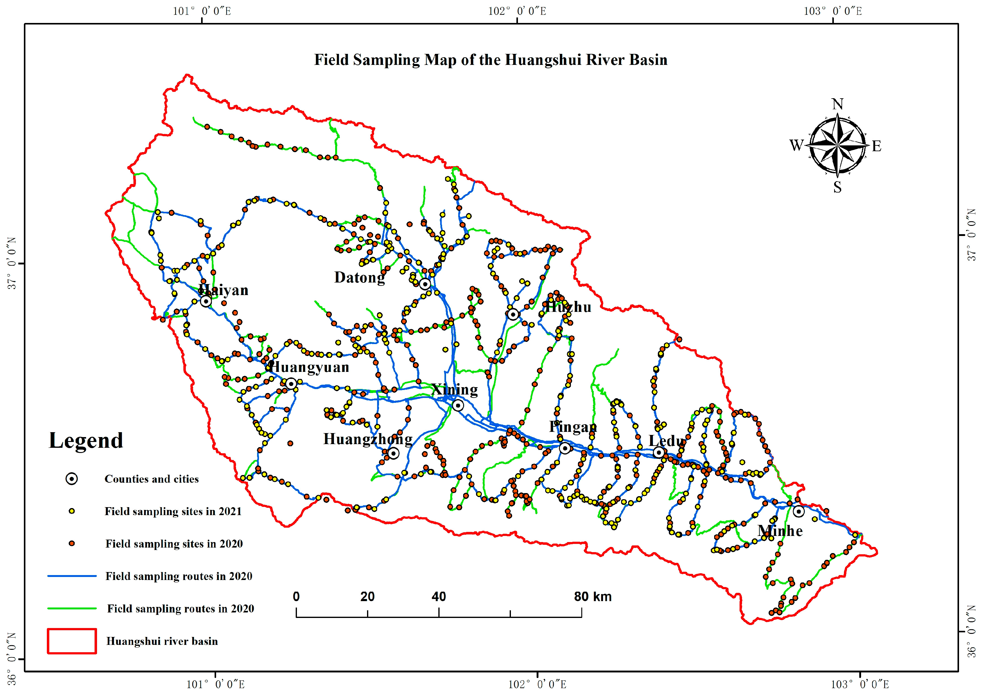
Due to the phenomena of “different spectra for the same object” and “different objects with the same spectrum”, it can be difficult to distinguish some features in an image. For example, arable land, nurseries, and orchards may appear very similar in an image, while the spectral characteristics of nurseries are very similar to those of sparse woodland. Therefore, another purpose of the fieldwork was to physically examine and verify the results of the feature classifications that could not be recognized in the images. The distribution of the field sampling points for the two years is shown in Figure 4, comprising a total of 824 sampling points and 6152 photographs.
Field sampling is limited by funding, complexity of the terrain, and road accessibility, so sample selection is dominated by the indoor collection of a large number of sample points of imagery. The accuracy and quantity of training sample selection usually have a large influence on the classification results. Niel et al. [48] showed that an increase in the number of samples has almost no effect on classification accuracy once the samples are sufficiently distributed throughout the whole image element, even when different classification methods are used. Considering that our study area has a large range and complex undulating terrain, significant differences in the area of each LULC type, and fragmented feature patches on the image, in order to select a sufficient number of samples to meet the classification requirements and reduce the impact of uneven sampling on the classification results, the sample selection was based on our field research combined with simultaneous high-definition Google Earth and Gaofen-1 satellite images. In our approach, visual interpretation was used to select samples, with a total of 12,160 samples chosen, including 1358 field samples and 10,802 indoor visual interpretation samples, encompassing 12 feature types.
The field sampling sites and route distribution maps are shown in Figure 4. The training samples and validation samples were divided according to a ratio of 7:3, with 8512 training samples and 3648 validation samples, respectively. The different LULC types in the samples are shown in Table 2.

4.1.2. Model Parameterization

In this paper, we used a PC configured with an IntelR CoreTM [email protected] processor, 16 GB of memory, and a 64-bit Windows 10 operating system. The classification code was executed in Python 3.6 within the IDE Pycharm development environment. The main libraries used in the computation process were the Geospatial Data Abstraction Library (GDAL); the machine learning Scikit-learn library, which provides a variety of classification, clustering, and regression algorithms including RF, SVM, GBDT, XGBoost, etc.; Python’s pandas (an extended program library for data analysis); numpy (an array arithmetic library); and time (including timing and temporal calculations, i.e., the time used for classification). These libraries allowed the code to read and write more than 200 types of raster data, and they contain various data processing functions that are widely used by researchers by virtue of their advantages of being powerful, free, open source, and supported by long-term maintenance [49].
The parameter settings for the three ensemble learning methods are shown in Table 3, where grid search was used to find the optimal values for each parameter.
The dataset classified in this study is large at 80 GB; however, GDAL only provides space for 2 GB [50], so using GDAL to read the dataset directly will overflow the memory, meaning it cannot be processed directly. Through various trials, it was found that the classification of sub-blocks could not be applied to the whole watershed at once because the classification accuracy of the whole watershed is not the simple average of the classification accuracy of each small block. In addition, the topography and feature complexity of each small block in the whole watershed are different, where some areas have complex and broken topography and smaller feature patches while other areas are flatter and have larger feature patches. Thus, the classifiers used for all sub-blocks are not the same; instead, a variety of classifiers is needed to classify the entire watershed. For example, using RF algorithms to classify the whole watershed, the whole image is divided into many small pieces, where a different RF model is used for each sub-block due to the different degrees of complexity and fragmentation in the study area. Consequently, the number of trees in the RF that is trained on each small area and the depths of the tree are different, which in turn requires a variety of different RF models for the whole area. Finally, the classification results for all sub-blocks are spliced together, where the classification accuracy is the average of all subregions. In this approach, however, the classification results and accuracy are poor.
In view of this, we propose the idea of subtotal division. First, the algorithm reads the sample point data in chunks, trains the classification model as a whole, and then classifies the entire region back into chunks. As we show below, this approach allowed us to classify the watershed successfully. The main steps of our process are (1) reading in chunks because GDAL memory is limited, (2) dividing the image into many small chunks, (3) reading the sample point data and the corresponding LULC type of each small chunk and combine the samples together. (4) storing the read values in a list, (5) cycling through the reads in turn, (6) reading the sample values and the LULC type data to train the classifier using all the samples, (7) storing the trained model, and (8) classifying the whole watershed in chunks with the trained model. This process continues until classification of the whole watershed is completed. This method trains the classifier using the whole watershed with all samples, producing consistently good results that are accurate and reasonable.

4.2. Classification Results

Assessment of Mapping Accuracy

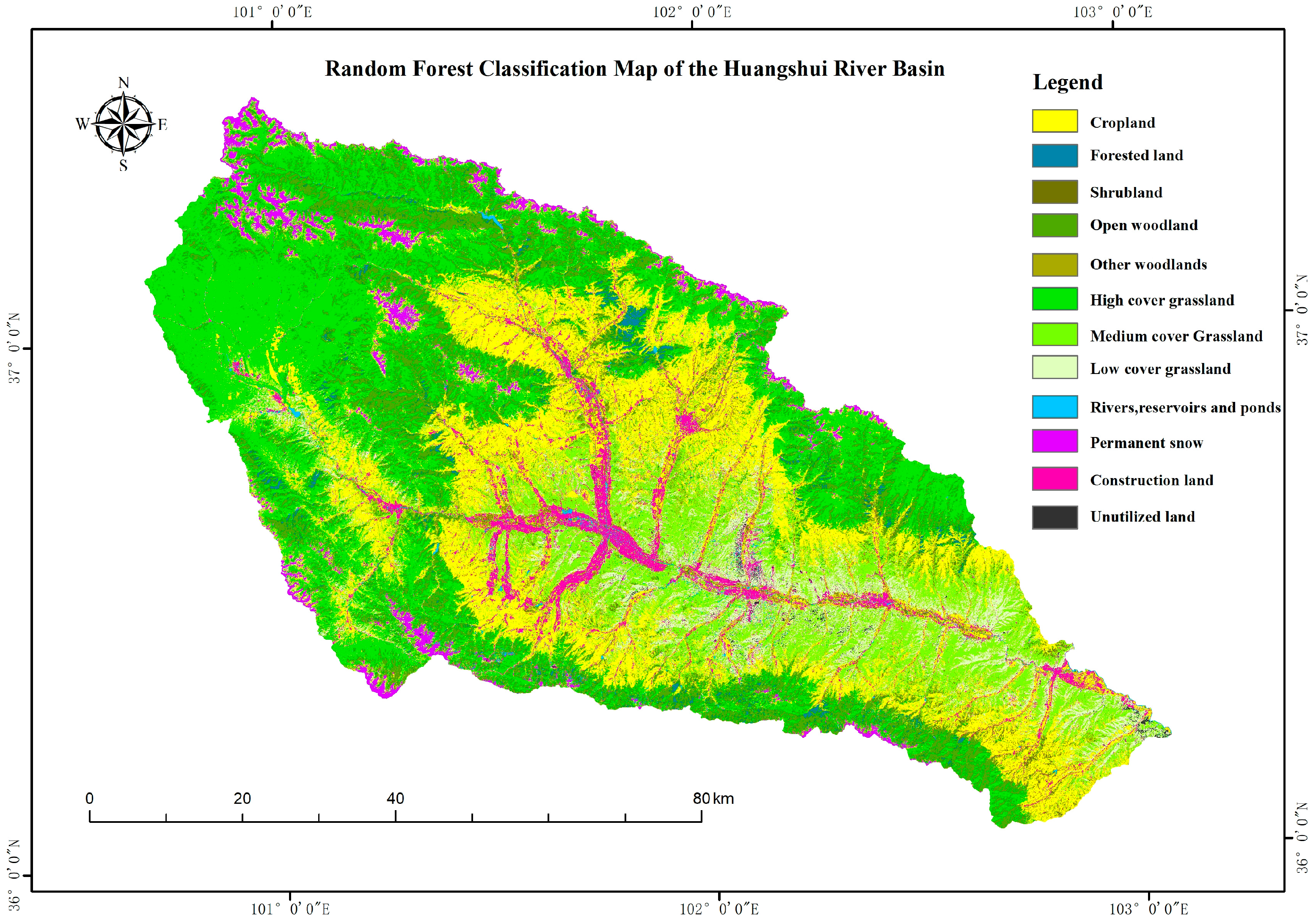
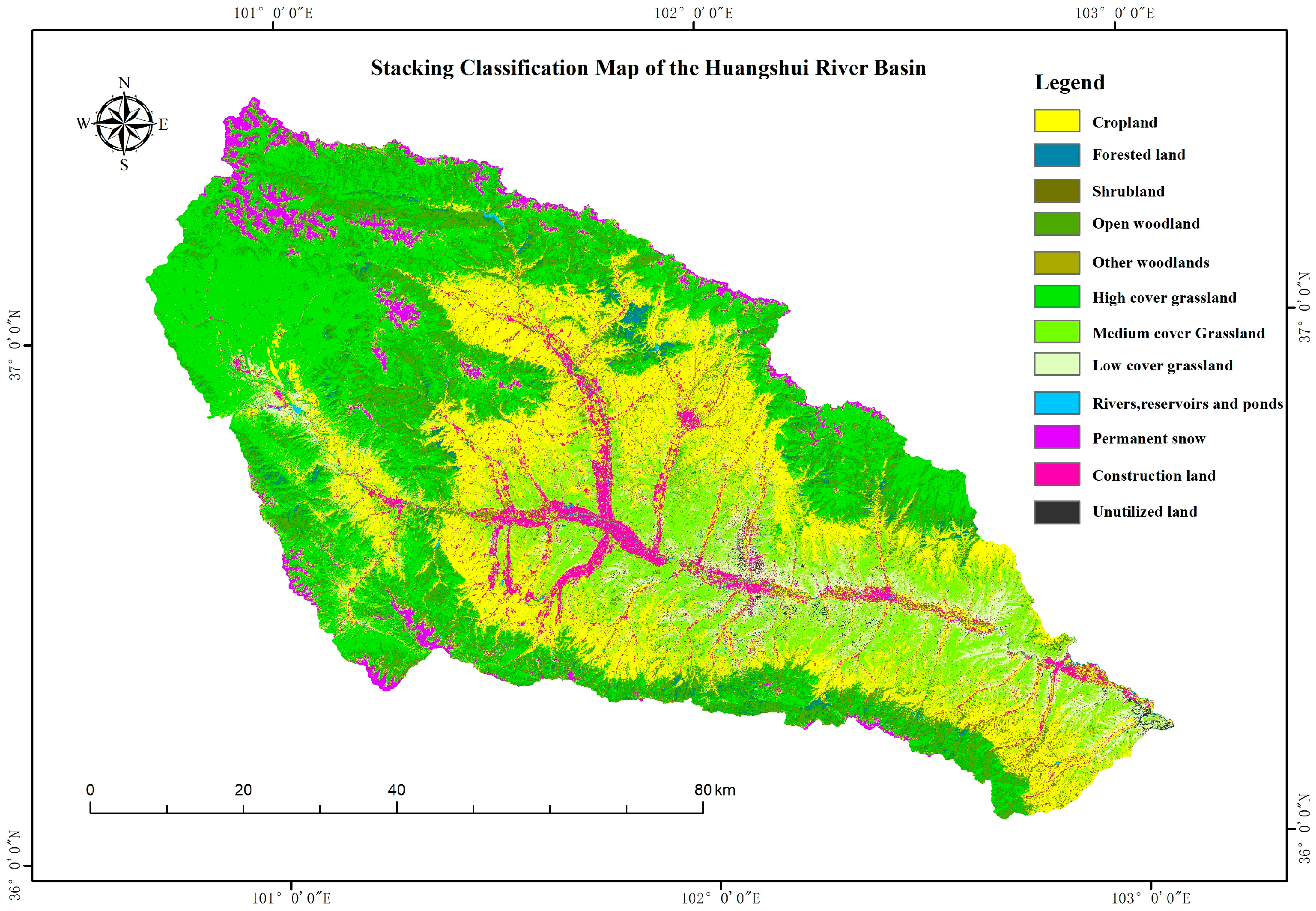
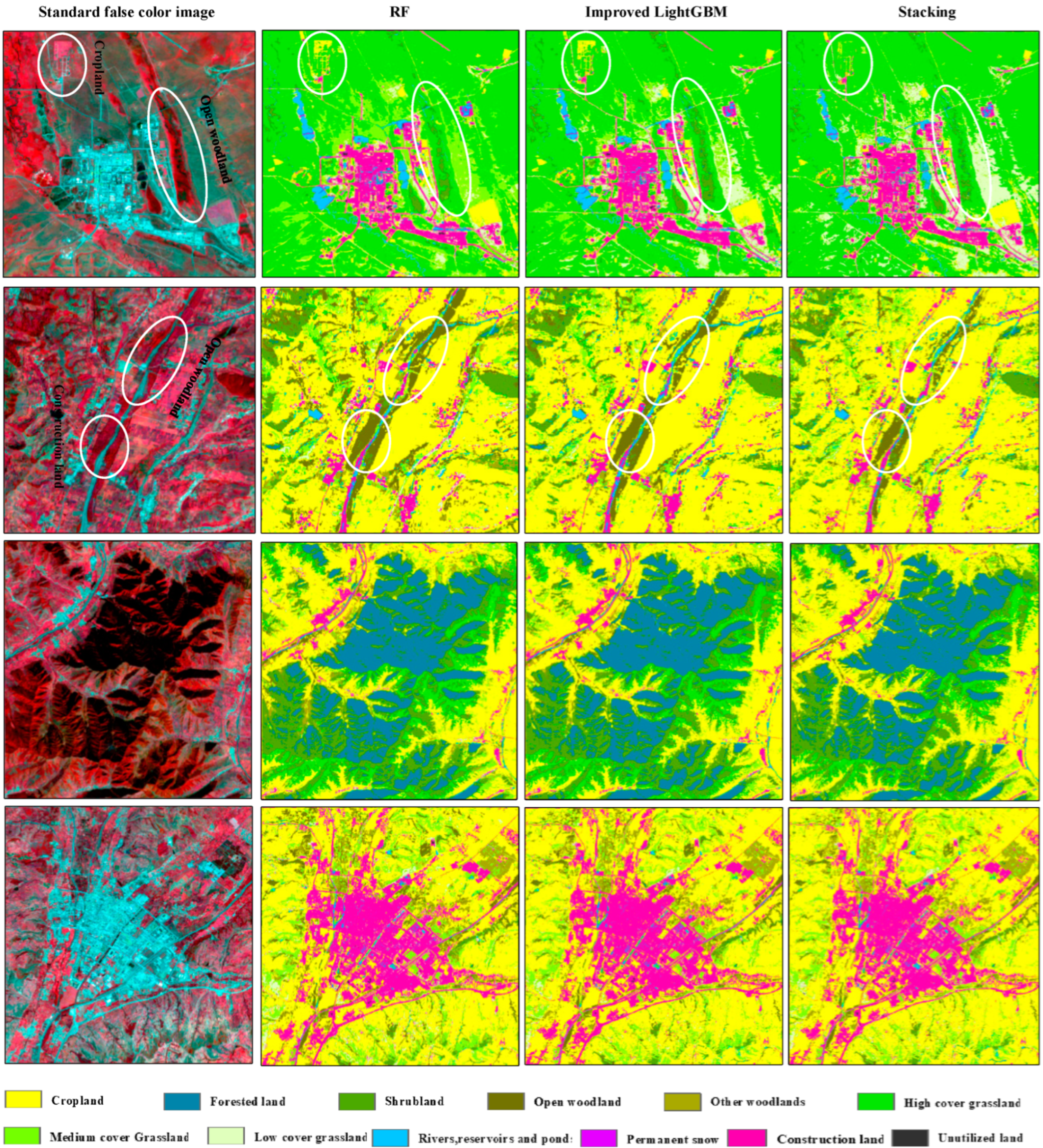
The classification results obtained using the optimal parameters through grid search of RF, the improved LightGBM, and stacking classification algorithms for LULC classification of the Huangshui watershed are shown in Figure 5, Figure 6 and Figure 7, respectively, while local details of the classification results are shown in Figure 8. The classification results were evaluated using the producer’s accuracy, user’s accuracy, F1-score, overall accuracy, and Kappa coefficient, as shown in Table 4, Table 5, Table 6 and Table 7 [51,52].
From the classification results presented in Figure 5, Figure 6 and Figure 7, it can be seen that the three ensemble algorithms each have a good classification effect, producing results that are consistent with the actual spatial distributions of LULC types determined via the field research. As can be seen in the three classification results, the differences in the spatial distribution and shape distribution of the features in the map are not very obvious. However, it can be seen that the RF algorithm and the stacking algorithm have more debris patches than the improved LightGBM algorithm, and the “salt and pepper” is obvious. Due to the different spatial sampling methods relative to the improved LightGBM algorithm, the information gain was calculated according to the sample point information. The information gain of a sample with a large gradient is larger than that of a sample with a smaller gradient. In our method, the sample with the large amount of information is retained and the sample with the least amount of information is removed. The information gradient of the image is large in the change of the feature type, and the gradient of the information within the feature is small, so the distribution of the features in the classification results has obvious boundaries and a clear contour. From the point of view of the spatial distribution of features, cultivated land in the whole basin is widely distributed, and all three algorithms were able to extract all of the cultivated land completely. Grasslands are distributed in a large area; construction land is mainly distributed in the plain area of river valleys; permanent snow is mainly distributed in the tops of Laji Mountain and Dabanshan Mountain, which have an elevation of more than 4000 m; and the unutilized land is sparsely distributed in the whole basin. The extraction effect of all algorithms was good for each of these LULC types.
From the detail map in Figure 8, it can be seen that there is almost no obvious difference between the three ensemble learning methods in terms of features that have a piecewise distribution over a large area. Due to the high classification accuracy of the three algorithms, good consistency is obtained in the classification detail maps. However, some features are quite fragmented, such as cultivated land and forests. We found that the improved LightGBM extracted clear object boundaries, while the RF and stacking algorithms gave poorer results. For urban residential land, all three algorithms were able to extract the land, but for rural settlements, RF and stacking failed to extract some rural settlements, while LightGBM extracted these settlements completely and their features were clearly outlined. As a whole, the RF and stacking algorithms produced more fragmented results, including the “pretzel phenomenon”, while the improved LightGBM algorithm gave better regional consistency. From in Figure 8, it can be seen that when the overall classification accuracy reached about 90%, the differences were very small in the spatial distributions of more regular and larger features, but in the area of more fragmented feature patches and more complex distribution of features, there were greater differences in the local details.
To illustrate the capabilities of the ensemble classification framework proposed in this study, each image of Huangshui Basin was divided into two blocks, dubbed region A and region B. However, due to the large amount of data in regions A and B, each was further divided into 341 smaller blocks where the geographic coordinates of the data of each small block and the corresponding LULC type were recorded. For each block, the read values were stored in a list. In total, 5389 sample points were used for region A, of which 3768 were training samples and 1621 were validation samples, while 3771 sample points, including 4743 training samples and 2028 validation samples, were used for region B.
In terms of classification accuracy, the RF model produced overall accuracies of 89.51% and 89.94% for classifications in region A and region B, respectively. The average overall accuracy was 89.73% for region A and region B, slightly higher than the overall accuracy of 88.76% obtained for the entire watershed. Tree depths of 10, 14, and 12 and 50, 80, and 200 leaf nodes were used for region A, region B, and the whole watershed, respectively. The overall accuracies of the improved LightGBM model were 89.64% and 91.62% for regions A and B, respectively. The average overall accuracy of 90.63% found for regions A and B was slightly less than the overall accuracy of 91.47% found for the entire watershed. Tree depths of 8, 10, and 7 and 40, 60, and 127 leaf nodes were used for region A, region B, and the whole watershed, respectively. The stacking model produced overall accuracies of 89.02% and 90.78% for regions A and B, respectively. The average overall accuracy was 89.90% for regions A and B, which is not equal to the overall accuracy of the whole watershed. Tree depths 10, 12, and 8 as well as 130, 150, and 150 leaf nodes were used for regions A and B, and the whole watershed, respectively. It can be seen that the classification results of the subregions are not equal to the classification results for the whole region, and the number and depths of the trees in the algorithms are obviously different.
Overall, the differences between block classification and overall classification are analyzed and compared, and the proposed LULC classification solution is a universal optimal mode at the watershed scale. Technically, block reading solves the problem of GDAL memory overflow.

4.3. Analysis of Variable Significance

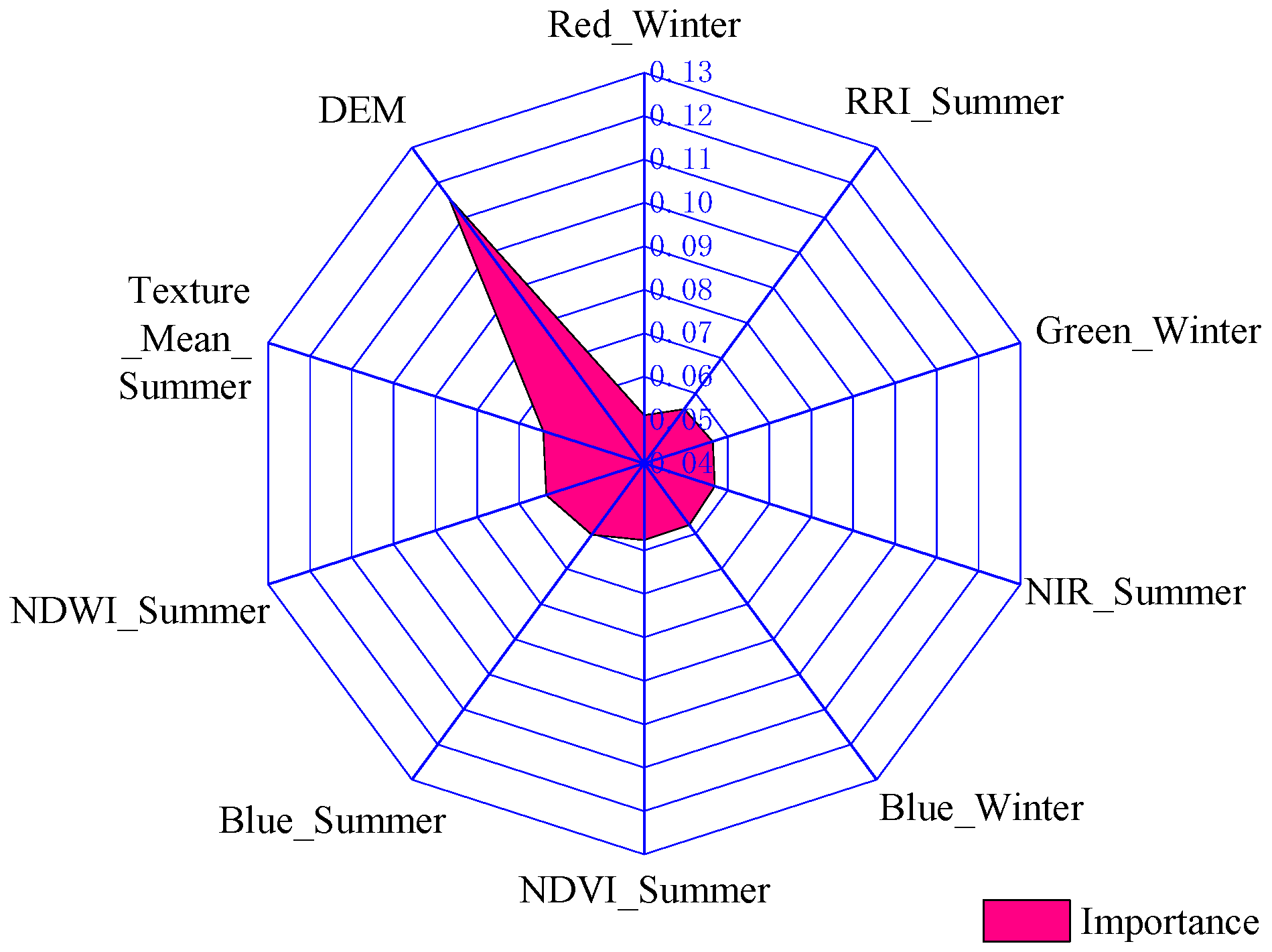
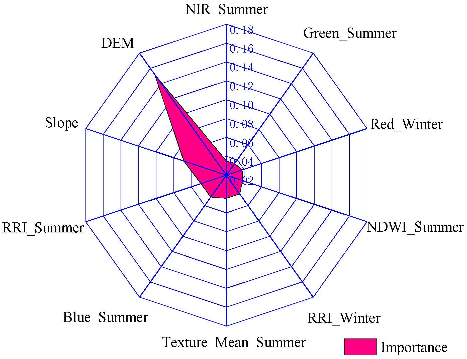
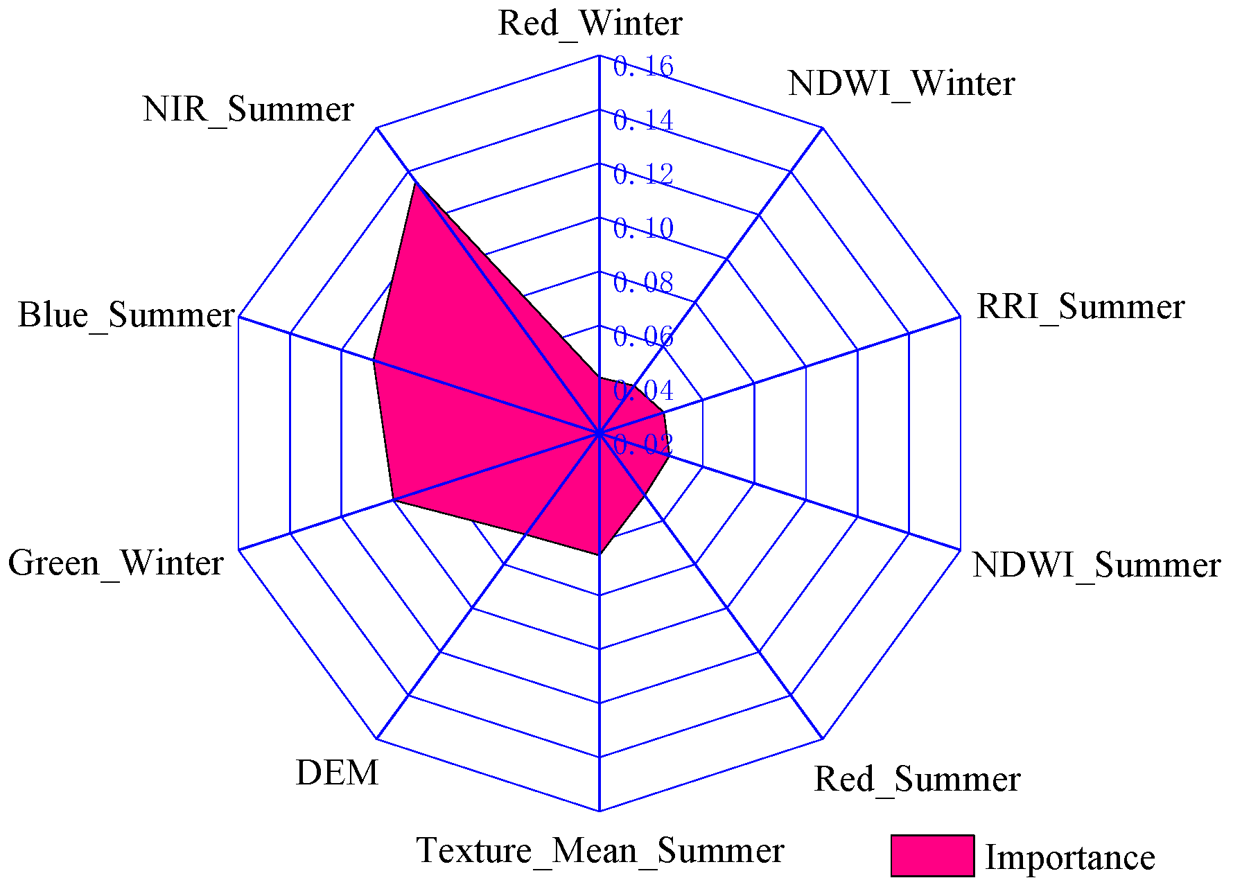
Since there are spectral features, index features, textural features, and terrain features in the classification dataset, in order to analyze the influence of each variable on the classification accuracy, the importance of each variable was calculated using the “feature_importances” method for the RF, improved LightGBM, and stacking algorithms. A top 10 ranking of importance is given for these three algorithms, respectively, in Figure 9, Figure 10 and Figure 11.
According to the top ten ranked variables, for all three algorithms, DEM is ranked in the top ten (ranked first for both RF and improved LightGBM), and the slope feature derived from DEM is ranked second for LightGBM; these results show that topographic factors are very important for the extraction of complex terrain areas. The original observing bands of winter and summer seasons are also important for the three algorithms, especially the near-infrared bands, which indicates that the original spectral features contain a lot of information. The NDVI, NDWI, and RRI indices in summer and winter are also very important in the extraction because they are indicative of the extraction of vegetation, water bodies, urban and rural industry, mining, and residential construction land. The mean value of the textural information is ranked in the top ten for the three algorithms, and the mean values of the eight textural features indicate the degree of regularity of the features, which are helpful for highlighting the edges and contours of features; this indicates that textural information also has a certain role in LULC information extraction. We note that similar conclusions were obtained in other studies [53,54].

5. Discussion

5.1. Advantages of the Classification Framework

The ensemble classification framework proposed in this study has five advantages: (1) Based on machine learning for LULC classification, much focus is typically placed on the classification results, such as classification accuracy, efficiency, and variable importance analysis, while the intermediate processes are often overlooked. This framework provides the intermediate processes of classification and offers an optimal classification model at the watershed scale. (2) The optimal results for model classification are achieved for all LULC types in the whole watershed, and only one classification model is needed for the entire watershed. If the model parameters are set in advance, then the parameters of the model in each sub-block are consistent, but the universal model does not reach the optimal result in the whole watershed. However, if the optimal parameters are searched for according to the training samples in each sub-block, the optimal results are reached in each module, thus necessitating the use of multiple models for the whole watershed. (3) The proposed framework reduces the influence of regional spatial variability within the watershed for the whole classification model, and the classification results obtained are holistic, macroscopic, and consistent. (4) Our method effectively has better classification accuracy. (5) Technically, block reading solves the memory overflow issue in GDAL. Based on our experiment for the Huangshui watershed, which achieved good LULC classification results, the classification framework can be replicated and be extended to other watersheds.
In addition, the extraction of LULC data should not only focus on the results but also the classification process itself. Most researchers focus exclusively on comparative studies of mapping methods, ignoring the process of categorization; in contrast, this study is a good illustration of the categorization process, provides an explanation of the mapping process, and is a complement to LULC mapping studies [55,56,57,58].

5.2. Effect of Different Methods on the Classification Results

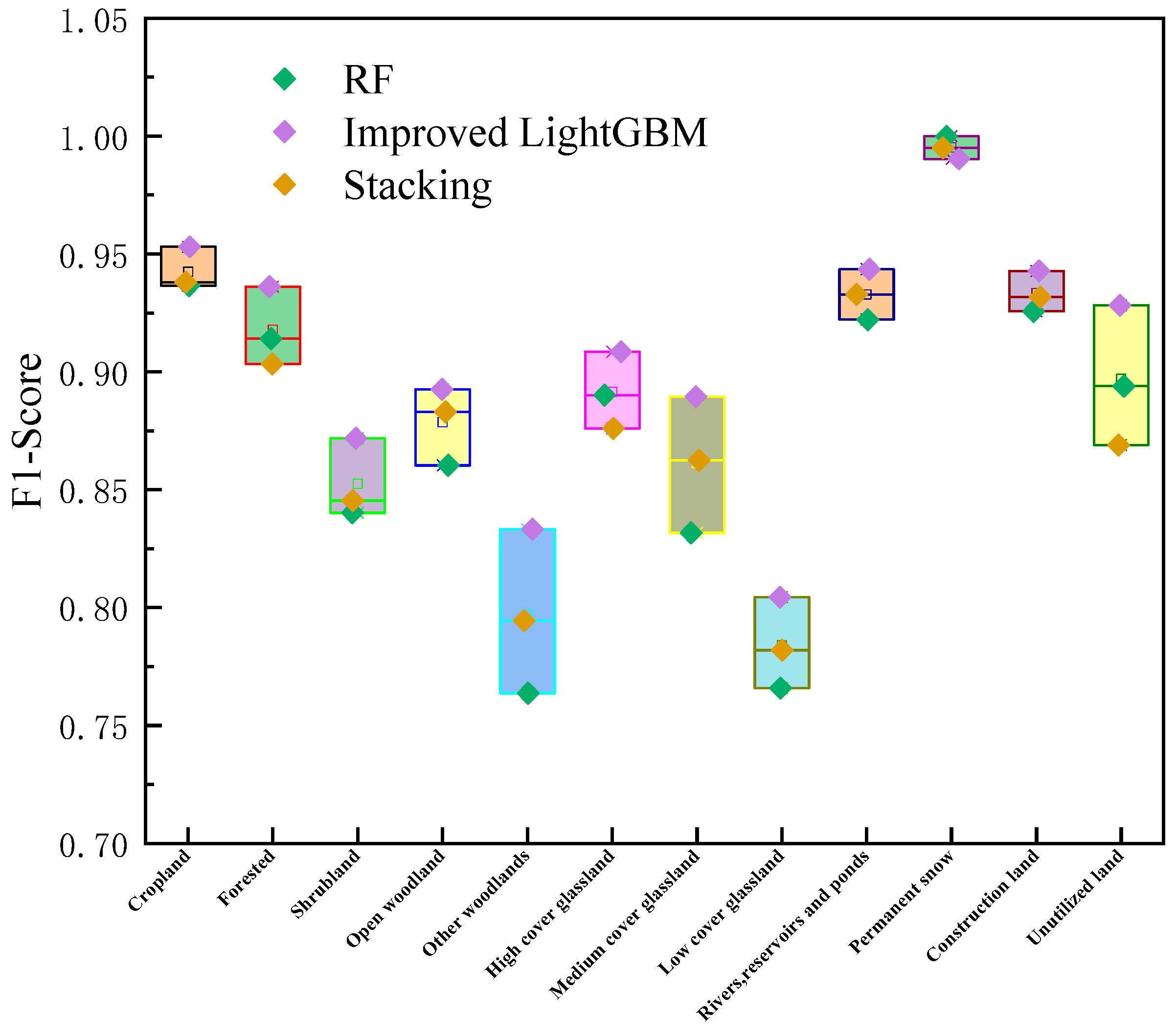
The F1-score is a reconciled average that combines the producer’s accuracy and user’s accuracy. By analyzing the F1-scores of different LULC types, we found that cultivated land, permanent snow, urban and rural industry, mining, and residential construction lands have high F1-scores. Meanwhile, other woodlands and low-cover grasslands showed lower F1-scores and were easily misclassified as cultivated land and thinned woodlands due to the fact that nurseries and cultivated land have the same geometric shapes and the same spectral characteristics as thinned woodland. Similarly, low-cover grassland was generally confused as medium-cover grassland and misclassified as unutilized land. It can be seen in Figure 12 that when the classification accuracy is higher, the classification method has little effect on improving the classification accuracy further, while for other forested land and low-covered grasslands with lower F1-scores, the classification method has a greater effect on improving the classification accuracy. For croplands, the F1-scores of the three ensemble algorithms were 0.94, 0.95, and 0.94, respectively, with a precision change of 0.01; the F1-scores of permanent snow were 1.00, 0.99, and 1.00, respectively, with a precision change of 0.01; and the F1-scores of urban and rural industry, mining, and residential construction land were 0.93, 0.94, and 0.93, respectively, with a precision of 0.01. However, for other forest lands, the F1-scores were 0.76, 0.83, and 0.79, respectively, and the precision changes were 0.07 and 0.04; and the F1-scores of low-cover grassland were 0.77, 0.80, and 0.78, respectively, and the precision changes were 0.03 and 0.02.
Our analysis has shown that when the accuracy of local LULC classification is high, the effect of different classification algorithms on the classification results is small, leading to precision changes of only 0.01; however, when the classification accuracy is low, the influence of different classification algorithms on the classification results is greater. In general, the classification methods follow the principle of diminishing returns in improving classification accuracy. The findings of this study are largely similar to those found in related works [41,58,59].

5.3. Classification Efficiency and Accuracy

In the entire watershed classification experiment, the computational time for RF was 7.57 h, while the improved LightGBM algorithm took 5.34 h and the stacking algorithm took 26.79 h. It is evident that the improved LightGBM is a more efficient algorithm in terms of computational time, whereas the stacking algorithm consumes considerable time, incurring a large computational cost.
Both RF and the improved LightGBM are based on the most popular bagging and boosting ensemble methods of decision trees. In this study, the improved LightGBM model outperformed the RF model due to differences in the ensemble methods of trees. RF uses the bagging (bootstrap sampling) method to construct different training sets and determines the final classification result by majority voting on results from different datasets. On the other hand, LightGBM employs the gradient boosting approach, a distributed computing algorithm based on decision trees, which has advantages in both computational efficiency and classification accuracy.
In this study, the improved LightGBM algorithm demonstrated superior classification accuracy and computational efficiency compared to the RF algorithm, indicating the superiority of boosting ensemble over bagging. This is consistent with the conclusions of related research [60,61]. Ensemble learning methods are stable algorithms that enhance the uncertainty of single classifier results through the interaction of multiple classifiers, thereby improving the accuracy of classification results. Overall, this also indicates that ensemble classifiers have certain advantages over single classifiers and complement each other, enhancing classification accuracy, consistent with the research findings of Feng et al. [62].
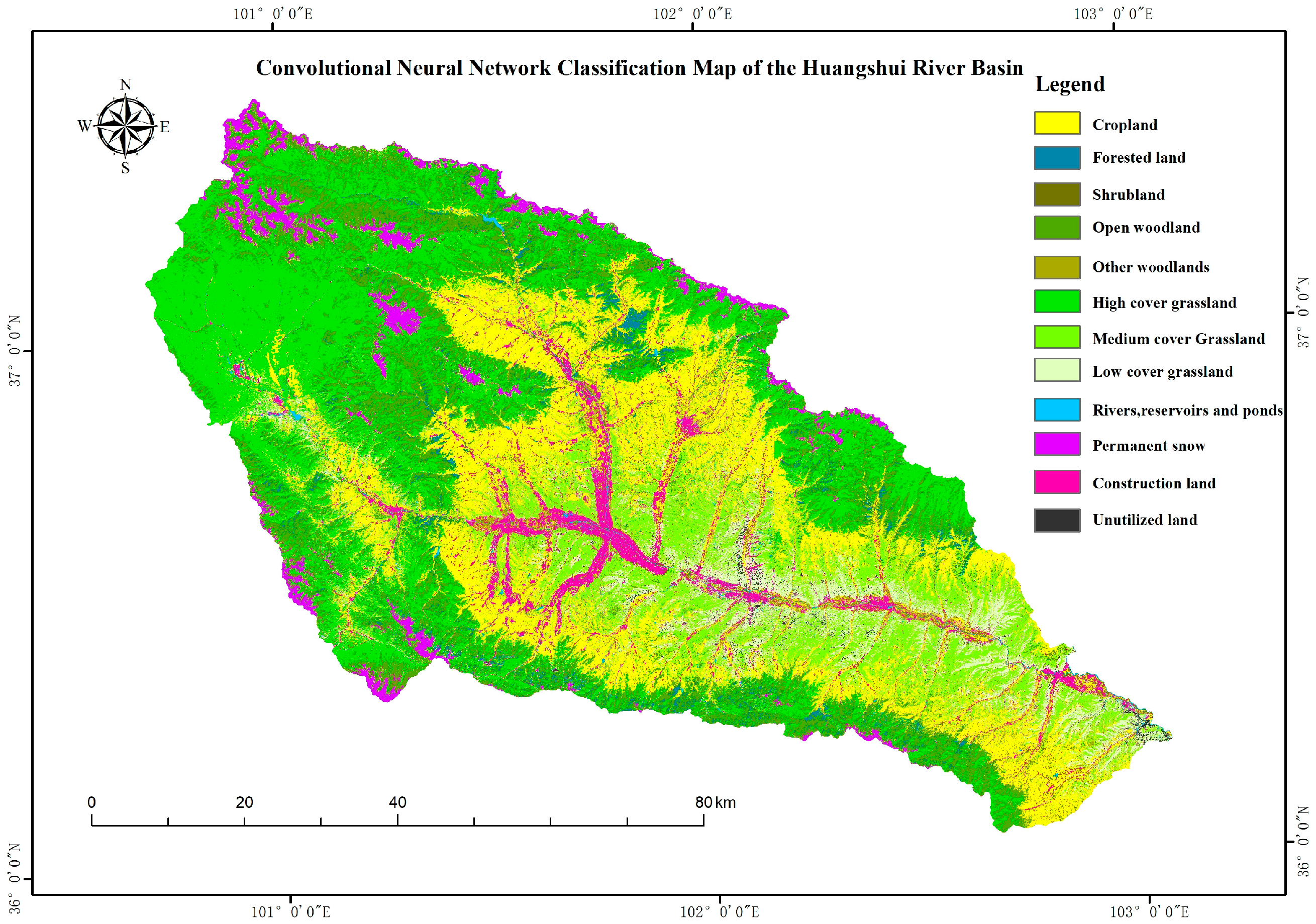
The classification of the Convolutional Neural Network (CNN) is shown in Figure 13. The overall classification accuracy of the CNN is 89.56%, with a Kappa coefficient of 0.8811, and the classification time is 32.76 h. Due to the high number of intermediate layers in deep learning, the convolutional and pooling processes are relatively time-consuming, resulting in lower computational efficiency compared to the ensemble classification methods used in this study. A detailed comparison with other models in the Huangshui watershed has been presented by our team members in another paper [63].

5.4. Comparison between Different Products

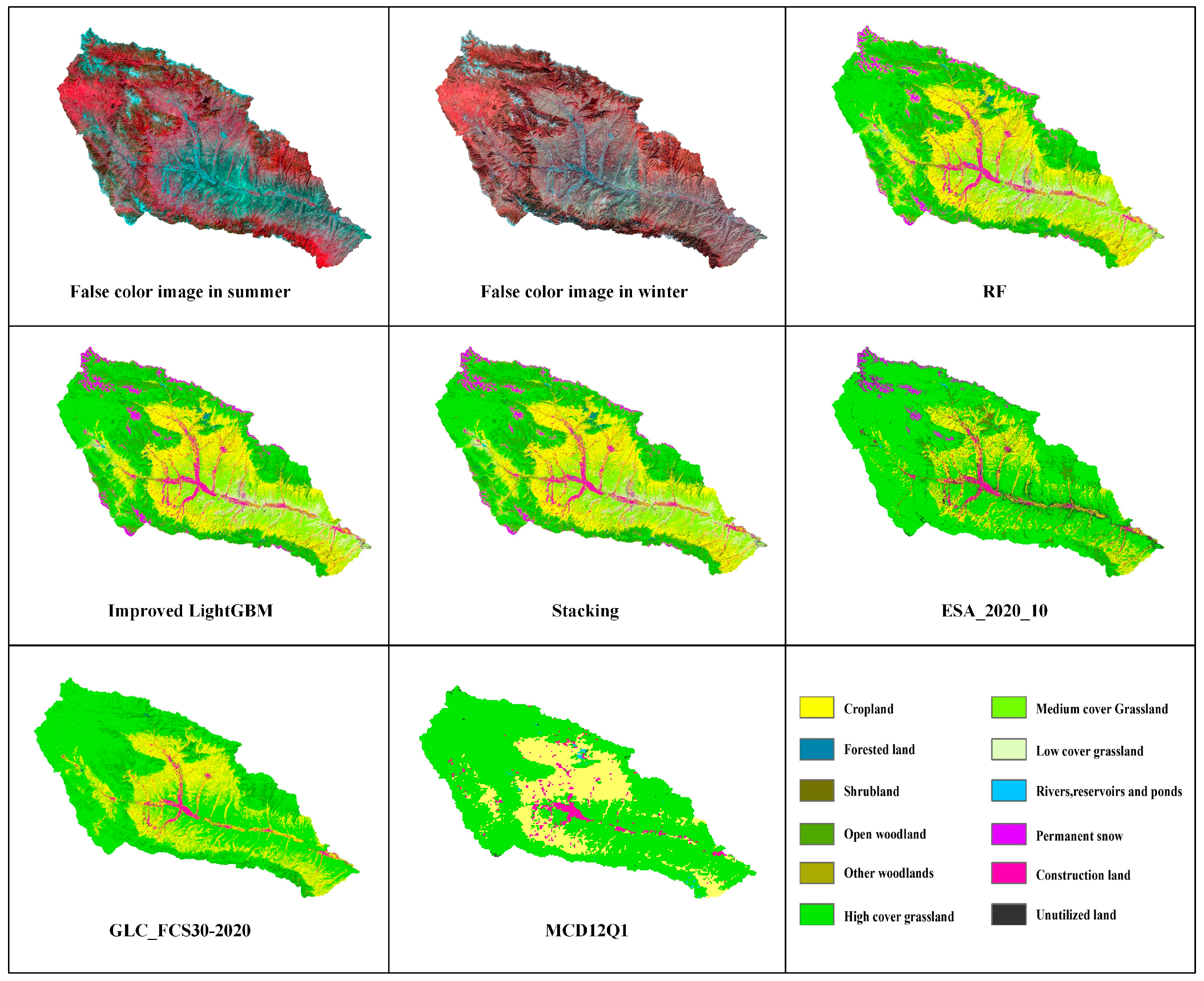
The classification results of the three ensemble algorithms in this paper are compared with the ESA_2020_10 product, GLC_FCS30-2020, and MCD12Q1, as shown in Figure 14.
The European Space Agency (ESA) jointly developed a global 10 m LULC product for the year 2020 with a number of research organizations around the world, and a comparison of the classification results of the three ensemble algorithms in this paper with the ESA_2020_10 product is shown in Figure 14. The overall accuracy of the ESA 10 m LULC products is 74.4%, with nine major categories, which is low compared to the classification accuracy of the three ensemble algorithms in this paper [64,65]. In comparison to the false color imagery, the ESA_2020_10 product for the river, reservoir pit, and pond classifications is basically consistent with this study. However, most of the sloping cultivated lands (hilly dry lands) and shrub forest lands were not extracted, the overall area of extracted construction land was small, the misclassification of unused land was relatively serious, grasslands were only extracted by the first-level classifier and were not subdivided by the second-level classifier, and some of the low-covered grasslands were misclassified as unused land, which erroneously implies that the total area of unused land is large. These results show that the LULC mapping approach employed in this study has certain advantages.
The research team led by Zhang et al. [22] from the Chinese Academy of Sciences’ Aerospace Information Research Institute has released the world’s first global 30 m land cover fine classification product for 2020. This dataset reflects the land cover distribution in global land areas (excluding Antarctica) at a spatial resolution of 30 m, providing up-to-date data support for land surface-related applications. It holds significant importance for global change analysis, sustainable development assessments, and monitoring of geographic conditions. The dataset builds on the 2015 Global Fine Land Cover Product (GLC_FCS30-2015) and incorporates Landsat surface reflectance data from 2019–2020, Sentinel-1 SAR data, DEM elevation data, global thematic auxiliary datasets, and prior knowledge datasets to produce the 2020 Global 30 m Fine Land Cover Product (GLC_FCS30-2020). Comparisons show that the extraction of farmland in the Huangshui watershed performed well, with the boundaries of grassland and forest being reasonably accurate; however, some rural residential points were not extracted.
The MCD12Q1 data is a MODIS land cover type product that provides annual land cover type distribution globally, with a resolution of 500 m. This data is obtained through supervised classification of reflectance data from the Terra and Aqua satellites, and specific categories are further optimized through post-processing and auxiliary information. The land cover dataset consists of a system made up of 17 different IGBP land use classification schemes [66]. Comparisons across the entire watershed reveal that many features were not extracted, resulting in poor overall detail.

6. Conclusions

Accurate and timely mapping of LULC types is crucial for research in agriculture and geoinformatics. In this study, we proposed an ensemble learning framework for watershed-scale LULC, which has improved accuracy and less irrationality than commonly used classification methods. Our approach uses the same model for LULC mapping across the entire watershed, which improves spatial consistency. We conducted experiments with three ensemble algorithms applied to the watershed, and a summary of the results follows.
(1) The subregion ensemble classification framework is a good technical method for processing big data for watershed-level LULC classification. Technically, block reading solves the memory overflow issue in GDAL.
(2) The classification accuracy and model parameters indicate that the results of block classification are not equal to the overall classification results. The proposed LULC classification solution is a universal optimal model at the entire watershed scale. Among the three ensemble learning methods, the improved LightGBM method is the optimal approach for LULC classification. Leveraging the complementary advantages of these methods through the ensemble classifier helps to improve the accuracy of LULC classification.
(3) The watershed-scale LULC products obtained in this study are superior to publicly available LULC products at the global scale.
Based on the performance of our algorithm in the Huangshui Basin area, the methodological framework proposed in this study can be easily applied to other similar basins, such as the Yellow River Basin and Yangtze River Basin. In the future, it will also be necessary to study AI mapping methods for multisource and multi-temporal data so that LULC mapping can be developed into a digital twin model encompassing AI and big data.

Author Contributions

Conceptualization, R.L. and X.G.; methodology, R.L.; software, R.L.; validation, F.S.; formal analysis, X.G.; investigation, R.L., X.G. and F.S.; resources, X.G.; data curation, F.S.; writing—original draft preparation, R.L.; writing—review and editing, R.L. and X.G.; supervision, X.G.; project administration, X.G.; and funding acquisition X.G. All authors have read and agreed to the published version of the manuscript.

Funding

This work is supported by the Natural Science Foundation of Qinghai Science and Technology Department (grant No. 2021-ZJ-913).

Data Availability Statement

The data presented in this study are available upon request from the first author.

Acknowledgments

We sincerely thank the anonymous reviewers for their insightful comments, which improved this manuscript.

Conflicts of Interest

The authors declare no conflicts of interest.

References

  1. Song, X.-P.; Hansen, M.C.; Stehman, S.V.; Potapov, P.V.; Tyukavina, A.; Vermote, E.F.; Townshend, J.R. Global land change from 1982 to 2016. Nature 2018, 560, 639–643. [Google Scholar] [CrossRef]
  2. Foley, J.A.; DeFries, R.; Asner, G.P.; Barford, C.; Bonan, G.; Carpenter, S.R.; Chapin, F.S.; Coe, M.T.; Daily, G.C.; Gibbs, H.K. Global consequences of land use. Science 2005, 309, 570–574. [Google Scholar] [CrossRef]
  3. Zhang, C.; Harrison, P.A.; Pan, X.; Li, H.; Sargent, I.; Atkinson, P.M. Scale Sequence Joint Deep Learning (SS-JDL) for land use and land cover classification. Remote Sens. Environ. 2020, 237, 111593. [Google Scholar] [CrossRef]
  4. Dang, V.H.; Hoang, N.D.; Nguyen, L.M.D.; Bui, D.T.; Samui, P. A novel GIS-based random forest machine algorithm for the spatial prediction of shallow landslide susceptibility. Forests 2020, 11, 118. [Google Scholar] [CrossRef]
  5. Szantoi, Z.; Geller, G.N.; Tsendbazar, N.E.; See, L.; Griffiths, P.; Fritz, S.; Gong, P.; Herold, M.; Mora, B.; Obregón, A. Addressing the need for improved land cover map products for policy support. Environ. Sci. Policy 2020, 112, 28–35. [Google Scholar] [CrossRef]
  6. Talukdar, S.; Singha, P.; Mahato, S.; Shahfahad; Pal, S.; Liou, Y.-A.; Rahman, A. Land-use land-cover classification by machine learning classifiers for satellite observations—A review. Remote Sens. 2020, 12, 1135. [Google Scholar] [CrossRef]
  7. Maxwell, A.E.; Warner, T.A.; Fang, F. Implementation of machine-learning classification in remote sensing: An applied review. Int. J. Remote Sens. 2018, 39, 2784–2817. [Google Scholar] [CrossRef]
  8. Adam, E.; Mutanga, O.; Odindi, J.; Abdel-Rahman, E.M. Land-use/cover classification in a heterogeneous coastal landscape using Rapid Eye imagery: Evaluating the performance of random forest and support vector machines classifiers. Int. J. Remote Sens. 2014, 35, 3440–3458. [Google Scholar] [CrossRef]
  9. Camargo, F.F.; Sano, E.E.; Almeida, C.M.; Mura, J.C.; Almeida, T.A. A comparative assessment of machine learning techniques for land use and land cover classification of the Brazilian tropical savanna using ALOS-2/PALSAR-2 polarimetric images. Remote Sens. 2019, 11, 1600. [Google Scholar] [CrossRef]
  10. Li, X.; Chen, W.; Cheng, X.; Wang, L. A comparison of machine learning algorithms for mapping of complexsurface-mined and agricultural landscapes using ZiYuan-3 stereo satellite imagery. Remote Sens. 2016, 8, 514. [Google Scholar] [CrossRef]
  11. Rogan, J.; Franklin, J.; Stow, D.; Miller, J.; Woodcock, C.; Roberts, D. Mapping land-cover modifications over large areas: A comparison of machine learning algorithms. Remote Sens. Environ. 2008, 112, 2272–2283. [Google Scholar] [CrossRef]
  12. Ma, L.; Li, M.; Ma, X.; Cheng, L.; Du, P.; Liu, Y. A review of supervised object-based land-cover image classification. ISPRS J. Photogramm. Remote Sens. 2017, 130, 277–293. [Google Scholar] [CrossRef]
  13. Shen, H.F.; Lin, Y.H.; Tian, Q.J.; Xu, K.; Jiao, J. A comparison of multiple classifier combinations using different voting-weights for remote sensing image classification. Int. J. Remote Sens. 2018, 39, 3705–3722. [Google Scholar] [CrossRef]
  14. Wen, L.; Hughes, M. Coastal wetland mapping using ensemble learning algorithms: A comparative study of Bagging, Boosting and Stacking techniques. Remote Sens. 2020, 12, 1683. [Google Scholar] [CrossRef]
  15. Feng, S.; Li, W.; Xu, J.; Liang, T.; Ma, X.; Wang, W.; Yu, H. Land use/land cover mapping based on GEE for the monitoring of changes in ecosystem types in the upper Yellow River basin over the Tibetan Plateau. Remote Sens. 2022, 14, 5361. [Google Scholar] [CrossRef]
  16. Gislason, P.O.; Benediktsson, J.A.; Sveinsson, J.R. Random forests for land cover classification. Pattern Recognit. Lett. 2006, 27, 294–300. [Google Scholar] [CrossRef]
  17. Chan, J.C.W.; Paelinckx, D. Evaluation of random forest and adaboost tree-based ensemble classification and spectral band selection for ecotope mapping using airborne hyper-spectral imagery. Remote Sens. Environ. 2008, 112, 2999–3011. [Google Scholar] [CrossRef]
  18. Yang, L.; Mansaray, L.; Huang, J.; Wang, L. Optimal segmentation scale parameter, feature subset and classification algorithm for geographic object-based crop recognition using multisource satellite imagery. Remote Sens. 2019, 11, 514. [Google Scholar] [CrossRef]
  19. Abdullah, A.Y.M.; Masrur, A.; Adnan, M.S.G.; Baky, M.A.A.; Hassan, Q.K.; Dewan, A. Spatio-temporal patterns of land use/land cover change in the heterogeneous coastal region of bangladesh between 1990 and 2017. Remote Sens. 2019, 11, 790. [Google Scholar] [CrossRef]
  20. Tian, Z.; Wei, J.; Li, Z. How important is satellite-retrieved aerosol optical depth in deriving surface PM2.5 using machine learning. Remote Sens. 2023, 15, 3780. [Google Scholar] [CrossRef]
  21. Zhang, P.; Hu, S.G.; Li, W.D.; Zhang, C.; Cheng, P. Improving parcel-level mapping of smallholder crops from VHSR imagery: An ensemble machine-learning-based framework. Remote Sens. 2021, 13, 2146. [Google Scholar] [CrossRef]
  22. Zhang, X.; Zhao, T.; Xu, H.; Liu, W.; Wang, J.; Chen, X.; Liu, L. GLC_FCS30D: The first global 30 m land-cover dynamics monitoring product with a fine classification system for the period from 1985 to 2022 generated using dense-time-series Landsat imagery and the continuous change-detection method. Earth Syst. Sci. Data 2024, 16, 1353–1381. [Google Scholar] [CrossRef]
  23. Herold, M.; Mayaux, P.; Woodcock, C.E.; Baccini, A.; Schmullius, C. Some challenges in global land cover mapping: An assessmentof agreement and accuracy in existing 1 km datasets. Remote Sens. Environ. 2008, 112, 2538–2556. [Google Scholar] [CrossRef]
  24. Kaptué Tchuenté, A.T.; Roujean, J.-L.; De Jong, S.M. Comparison and relative quality assessment of the GLC2000, GLOBCOVER, MODIS and ECOCLIMAP land cover data sets at the African continental scale. Int. J. Appl. Earth Obs. Geoinf. 2011, 13, 207–219. [Google Scholar] [CrossRef]
  25. Mou, X.L.; Li, H.; Huang, C.; Liu, Q.; Liu, G. Application progress of google earth engine in land use and land cover remote sensing information extraction. Remote Sens. Land Resour. 2021, 33, 1–10. [Google Scholar]
  26. Wang, F.F.; Liu, S.; Liu, Y.; Sun, Y.; Yu, L.; Wang, Q.; Dong, Y.; Beazley, R. Long-term dynamics of nitrogen flow in a typical agricultural and pastoral region on the Qinghai-Tibet Plateau and its optimization strategy. Environ. Pollut. 2021, 288, 117684. [Google Scholar] [CrossRef]
  27. Ghorbanian, A.; Zaghian, S.; Asiyabi, R.M.; Amani, M.; Mohammadzadeh, A.; Jamali, S. Mangrove ecosystem mapping using sentinel-1 and sentinel-2 satellite images and random forest algorithm in google earth engine. Remote Sens. 2021, 13, 2565. [Google Scholar] [CrossRef]
  28. Caballero, I.; Navarro, G. Monitoring cyanoHABs and water quality in Laguna Lake (Philippines) with sentinel-2 satellites during the 2020 Pacific typhoon season. Sci. Total Environ. 2021, 788, 147700. [Google Scholar] [CrossRef]
  29. Vizzari, M. Planet scope, sentinel-2, and sentinel-1 data integration for object-based land cover classification in google earth engine. Remote Sens. 2022, 14, 2628. [Google Scholar] [CrossRef]
  30. Pott, L.P.; Amado, T.J.C.; Schwalbert, R.A.; Corassa, G.M.; Ciampitti, I.A. Satellite-based data fusion crop type classification andmapping in Rio Grande do Sul, Brazil. ISPRS J. Photogramm. Remote Sens. 2021, 176, 196–210. [Google Scholar] [CrossRef]
  31. Verde, N.; Kokkoris, I.P.; Georgiadis, C.; Kaimaris, D.; Dimopoulos, P.; Mitsopoulos, I.; Mallinis, G. National scale land coverclassification for ecosystem services mapping and assessment, using multitemporal copernicus EO data and google earth engine. Remote Sens. 2020, 12, 3303. [Google Scholar] [CrossRef]
  32. Tuvdendorj, B.; Zeng, H.; Wu, B.; Elnashar, A.; Zhang, M.; Tian, F.; Nabil, M.; Nanzad, L.; Bulkhbai, A.; Natsagdorj, N. Performance and the optimal integration of sentinel-1/2 time-series features for crop classification in Northern Mongolia. Remote Sens. 2022, 14, 1830. [Google Scholar] [CrossRef]
  33. Fremout, T.; Cobián-De Vinatea, J.; Thomas, E.; Huaman-Zambrano, W.; Salazar-Villegas, M.; Limache-de la Fuente, D.; Bernardino, P.N.; Atkinson, R.; Csaplovics, E.; Muys, B. Site-specific scaling of remote sensing-based estimates of woody cover and aboveground biomass for mapping long-term tropical dry forest degradation status. Remote Sens. Environ. 2022, 276, 113040. [Google Scholar] [CrossRef]
  34. Amini, S.; Saber, M.; Rabiei-Dastjerdi, H.; Homayouni, S. Urban land use and land cover change analysis using random forest classification of landsat time series. Remote Sens. 2022, 14, 2654. [Google Scholar] [CrossRef]
  35. Tucker, C.J. Red and photographic infrared linear combinations for monitoring vegetation. Remote Sens. Environ. 1979, 8, 127–150. [Google Scholar] [CrossRef]
  36. Gao, B.-C. NDWI—A normalized difference water index for remote sensing of vegetation liquid water from space. Remote Sens. Environ. 1996, 58, 257–266. [Google Scholar] [CrossRef]
  37. Ji, H.; Li, X.; Wei, X.; Liu, W.; Zhang, L.; Wang, L. Mapping 10-m resolution rural settlements using multi-source remote sensing datasets with the google earth engine platform. Remote Sens. 2020, 12, 2832. [Google Scholar] [CrossRef]
  38. Johansen, K.; Phinn, S. Mapping structural parameters and species composition of riparian vegetation using IKONOS and Landsat ETM+ data in Australian tropical savannahs. Photogramm. Eng. Remote Sens. 2006, 72, 71–80. [Google Scholar] [CrossRef]
  39. Fassnacht, F.E.; Latifi, H.; Stere’nczak, K.; Modzelewska, A.; Lefsky, M.; Waser, L.T.; Straub, C.; Ghosh, A. Review of studies on tree species classification from remotely sensed data. Remote Sens. Environ. 2016, 186, 64–87. [Google Scholar] [CrossRef]
  40. Mohammadpour, P.; Viegas, D.X.; Viegas, C. Vegetation mapping with random forest using sentinel 2 and GLCM texture feature—A case study for Lousã Region, Portugal. Remote Sens. 2022, 14, 4585. [Google Scholar] [CrossRef]
  41. Yang, Y.; Yang, D.; Wang, X.; Zhang, Z.; Nawaz, Z. Testing accuracy of land cover classification algorithms in the qilian mountains based on gee cloud platform. Remote Sens. 2021, 13, 5064. [Google Scholar] [CrossRef]
  42. Mariana, B.; Lucian, D. Random forest in remote sensing: A review of applications and future directions. ISPRS J. Photogramm. Remote Sens. 2016, 114, 21–31. [Google Scholar]
  43. Freund, Y.; Schapire, R.E. A decision-theoretic generalization of on-line learning and an application to boosting. J. Comput. Syst. Sci. 1997, 55, 119–139. [Google Scholar] [CrossRef]
  44. Chen, T.; Guestrin, C. XGBoost: A scalable tree boosting system. In Proceedings of the 22nd ACM SIGKDD International Conference on Knowledge Discovery and Data Mining, San Francisco, CA, USA, 13–17 August 2016; pp. 785–794. [Google Scholar]
  45. Zhang, J.; Xu, J.; Dai, X.; Ruan, H.; Liu, X.; Jing, W. Multi-source precipitation data merging for heavy rainfall events based on CoKriging and machine learning methods. Remote Sens. 2022, 14, 1750. [Google Scholar] [CrossRef]
  46. Chai, X.; Li, J.; Zhao, J.; Wang, W.; Zhao, X. LGB-PHY: An evaporation duct height prediction model based on physically constrained LightGBM algorithm. Remote Sens. 2022, 14, 3448. [Google Scholar] [CrossRef]
  47. Cheng, X.; Lei, H. Remote sensing scene image classification based on mmsCNN–HMM with stacking ensemble model. Remote Sens. 2022, 14, 4423. [Google Scholar] [CrossRef]
  48. Van Niel, T.G.; Mcvicar, T.; Datt, B. On the relationship between training sample size and data dimensionality: Monte Carlo analysis of broadband multi-temporal classification. Remote Sens. Environ. 2005, 98, 468–480. [Google Scholar] [CrossRef]
  49. Appel, M.; Lahn, F.; Buytaert, W.; Pebesma, E. Open and scalable analytics of large Earth observation datasets: From scenes to multidimensional arrays using SciDB and GDAL. ISPRS J. Photogramm. Remote Sens. 2018, 138, 47–56. [Google Scholar] [CrossRef]
  50. Zhang, H.; Tong, H.; Zuo, B.; Zhang, X. Quick browsing of massive remote sensing image based on GDAL. Comput. Eng. Appl. 2012, 48, 159–162. [Google Scholar]
  51. Congalton, R.G. A review of assessing the accuracy of classifications of remotely sensed data. Remote Sens. Environ. 1991, 37, 35–46. [Google Scholar] [CrossRef]
  52. Foody, G.M. Status of land cover classification accuracy assessment. Remote Sens. Environ. 2002, 80, 185–201. [Google Scholar] [CrossRef]
  53. Haralick, R.M.; Shanmugam, K.; Dinstein, I.H. Textural features for image classification. IEEE Trans. Syst. Man Cybern. 1973, SMC-3, 610–621. [Google Scholar] [CrossRef]
  54. Kupidura, P. The comparison of different methods of texture analysis for their efficacy for land use classification in satelliteimagery. Remote Sens. 2019, 11, 1233. [Google Scholar] [CrossRef]
  55. Burai, P.; Deák, B.; Valkó, O.; Tomor, T. Classification of herbaceous vegetation using airborne hyperspectral imagery. Remote Sens. 2015, 7, 2046–2066. [Google Scholar] [CrossRef]
  56. Ghayour, L.; Neshat, A.; Paryani, S.; Shahabi, H.; Shirzadi, A.; Chen, W.; Al-Ansari, N.; Geertsema, M.; Pourmehdi Amiri, M.; Gholamnia, M.; et al. Performance evaluation of Sentinel-2 and Landsat 8 OLI Data for Land Cover/Use Classification Using a Comparison between Machine Learning Algorithms. Remote Sens. 2021, 13, 1349. [Google Scholar] [CrossRef]
  57. Saboori, M.; Homayouni, S.; Shah-Hosseini, R.; Zhang, Y. Optimum feature and classifier selection for accurate urban land use/cover mapping from very high resolution satellite imagery. Remote Sens. 2022, 14, 2097. [Google Scholar] [CrossRef]
  58. Rapinel, S.; Mony, C.; Lecoq, L.; Clement, B.; Thomas, A.; Hubert-Moy, L. Evaluation of Sentinel-2 time-series for mapping floodplain grassland plant communities. Remote Sens. Environ. 2019, 223, 115–129. [Google Scholar] [CrossRef]
  59. Ji, Q.; Liang, W.; Fu, B.; Zhang, W.; Yan, J.; Lü, Y.; Yue, C.; Jin, Z.; Lan, Z.; Li, S. Mapping land use/cover dynamics of the Yellow River Basin from 1986 to 2018 supported by Google Earth Engine. Remote Sens. 2021, 13, 1299. [Google Scholar] [CrossRef]
  60. Dietterich, T.G. An experimental comparison of three methods for constructing ensembles of decision trees: Bagging, boosting, and randomization. Mach. Learn. 2000, 40, 139–157. [Google Scholar] [CrossRef]
  61. Ghimire, B.; Rogan, J.; Rodríguez-Galiano, V.F.; Panday, P.; Neeti, N. An evaluation of bagging, boosting, and random forests for land-cover classification in Cape Cod, Massachusetts, USA. GIScience Remote Sens. 2012, 49, 623–643. [Google Scholar] [CrossRef]
  62. Feng, L.; Zhang, Z.; Ma, Y.; Du, Q.; Williams, P.; Drewry, J.; Luck, B. Alfalfa yield prediction using UAV-based hyperspectral imagery and ensemble learning. Remote Sens. 2020, 12, 2028. [Google Scholar] [CrossRef]
  63. Shi, F.; Gao, X.; Li, R.; Zhang, H. Ensemble Learning for the Land Cover Classification of Loess Hills in the Eastern Qinghai–Tibet Plateau Using GF-7 Multitemporal Imagery. Remote Sens. 2024, 16, 2556. [Google Scholar] [CrossRef]
  64. Venter, Z.S.; Barton, D.N.; Chakraborty, T.; Simensen, T.; Singh, G. Global 10 m land use land cover datasets: A comparison of Dynamic World, World Cover and Esri Land Cover. Remote Sens. 2022, 14, 4101. [Google Scholar] [CrossRef]
  65. Wang, X.; Zhang, Y.; Zhang, K. Automatic 10 m Forest Cover Mapping in 2020 at China’s Han River Basin by Fusing ESA Sentinel-1/Sentinel-2 Land Cover and Sentinel-2 near Real-Time Forest Cover Possibility. Forests 2023, 14, 1133. [Google Scholar] [CrossRef]
  66. Koyama, A.; Fukue, K.; Otake, Y.; Matsuoka, Y.; Hasegawa, T.; Hiyama, T.; Kato, H. Global land cover classification using modis surface reflectance prosucts. In Proceedings of the Asian Conference on Remote Sensing, Quezon City, Metro Manila, Philippines, 24–28 October 2015. [Google Scholar]
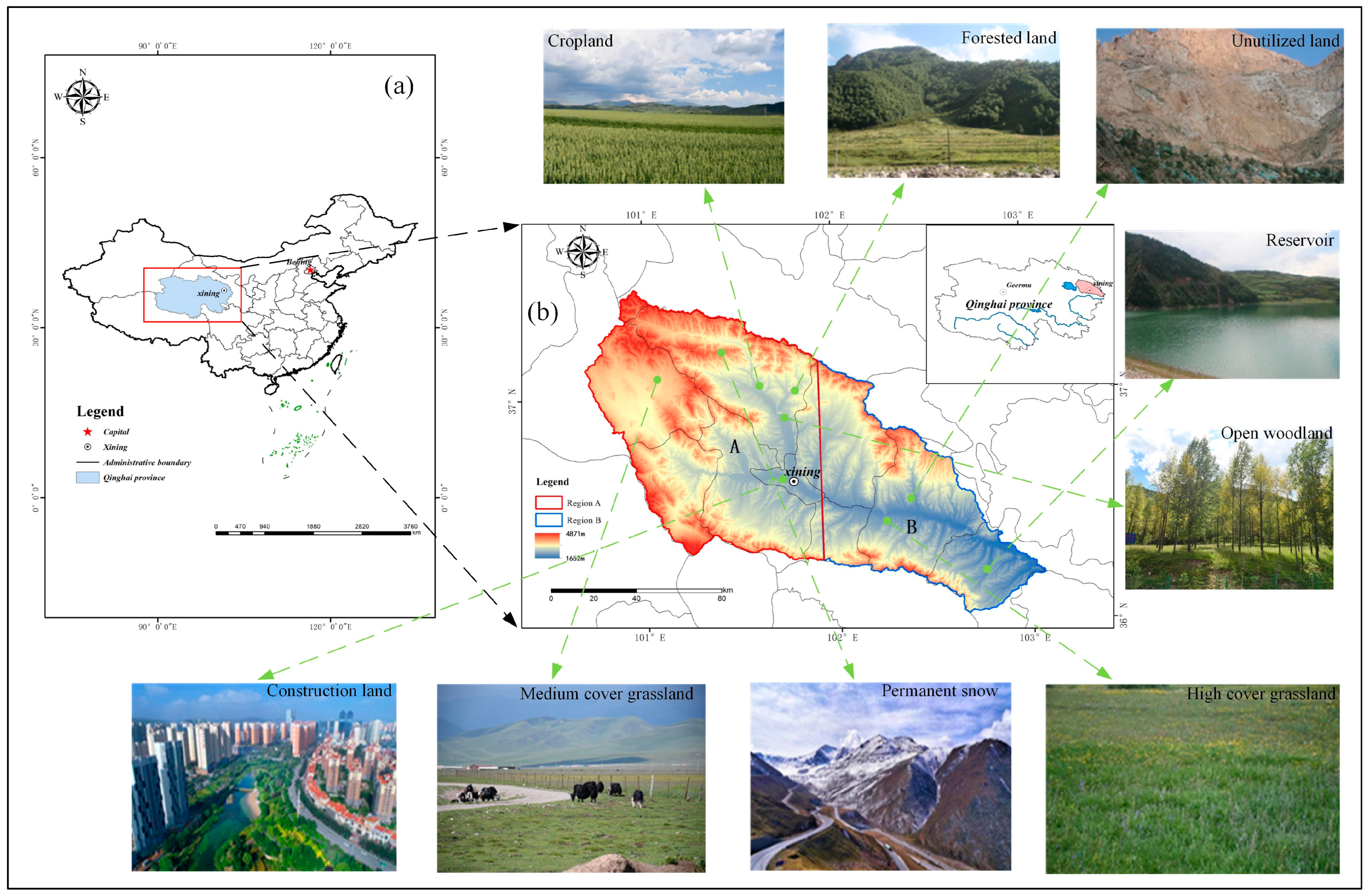
Figure 1. Map of the study area. (a) The location of Qinghai Province in China. (b) Map of the Location of the Huangshui River Basin in Qinghai Province (In figure (b), A and B represent two subdivisions).
Remotesensing 16 03855 g001
Figure 2. Statistics of the number of scenes used in the study.
Remotesensing 16 03855 g002
Figure 3. Flowchart of the LULC mapping strategy used in this study. (1) Data sources; (2) Categorical datase; (3) Classification methods and processes; (4) Classification results and evaluation.
Remotesensing 16 03855 g003
Figure 4. Field sampling routes and sites in 2020–2021.
Remotesensing 16 03855 g004
Figure 5. Raster map of RF classification results.
Remotesensing 16 03855 g005
Figure 6. Raster map of improved LightGBM classification results.
Remotesensing 16 03855 g006
Figure 7. Raster map of stacking classification results.
Remotesensing 16 03855 g007
Figure 8. Local details of the classification results. The white circles represent a detailed comparison of cropland and open woodland.
Remotesensing 16 03855 g008
Figure 9. Importance ranking of variables for the RF algorithm.
Remotesensing 16 03855 g009
Figure 10. Same as Figure 9, but for the improved LightGBM algorithm.
Remotesensing 16 03855 g010
Figure 11. Same as Figure 9, but for the stacking algorithm.
Remotesensing 16 03855 g011
Figure 12. F1-scores for the three ensemble algorithms.
Remotesensing 16 03855 g012
Figure 13. Raster map of CNN classification results.
Remotesensing 16 03855 g013
Figure 14. Comparison of different LULC in the Huangshui River basin in 2020.
Remotesensing 16 03855 g014
Table 1. Composition of the classification feature dataset.
DataWave BandDescriptiveQuantities
Primary bandsRedComposite images of summer and winter seasons.
Spatial resolution 10 m
8
Green
Blue
NIR
Spectral indicesNDVIReflects vegetation growth
Reflects the spatial distribution of water bodies
Reflects spatial distribution of buildings
6
NDWI
RRI
Texture featuresSecond MomentExtract the first principal component from the blue, green, red, and near-infrared bands and calculate the gray-level co-occurrence matrix from the first principal component, reflecting the texture information.16
Entropy
Variance
Contrast
Mean
Dissimilarity
Homogeneity
Correlation
Topographic featuresDEMReflects terrain elevation, slope, and aspect information3
Aspect
Slope
Table 2. The different LULC types in our dataset: training sample and validation sample.
LULC TypesNumber of Samples (Number)Training Samples (Number)Validation Sample (Number)
Cropland29052019886
Forested land526361165
Shrubland1044734310
Open woodland853594259
Other woodlands360239121
High-cover grassland1298932366
Medium-cover grassland1291896395
Low-cover grassland767535232
Rivers, reservoirs, and ponds821570251
Permanent snow364261103
Construction land15071084423
Unutilized land424287137
Total12,16085123648
Table 3. Hyperparameters of the classifier.
ClassifiersParametersDescriptionTuning Ranges
RFn_estimatorsThe number of trees, representing the number of iterations.1–500
max_featuresThe number of features to consider when looking for the best split.1–15
max_depthThe maximum depth of each tree.1–10
min_samples_splitThe minimum number of samples a node must have to be split.1–6
min_samples_leafThe minimum number of samples a leaf node must have.1–6
Improve LightGBMn_estimatorsThe number of trees, representing the number of iterations.1–500
learning_rateThe learning rate, controlling the update magnitude of model parameters in each iteration.0.01–0.1
boosting_typeThe parameter that specifies the type or strategy of the gradient boosting algorithm.“gbdt”
num_leavesThe number of leaf nodes.50–150
max_featuresThe number of features to consider when looking for the best split.1–10
max_depthThe maximum depth of each tree.1–10
min_samples_splitThe minimum number of samples a node must have to be split.1–5
min_samples_leafThe minimum number of samples a leaf node must have.1–5
L1Regularization parameter.0.1–0.5
L2Regularization parameter.0.1–0.5
Stackingnum_classNumber of classes.12
learning_rateThe learning rate, controlling the update magnitude of model parameters in each iteration.0.01–0.1
n_estimatorsThe number of trees, representing the number of iterations.250
max_depth The maximum depth of each tree.1–500
min_child_weightMinimum node weight.1–10
L1Regularization parameter.0.1–0.5
L2Regularization parameter.0.1–0.5
Table 4. Accuracy evaluation results of the three algorithms for the entire watershed.
LULC TypesRF AlgorithmImproved LightGBM AlgorithmStacking Algorithm
PA (%)UA (%)F1-ScorePA (%)UA (%)F1-ScorePA (%)UA (%)F1-Score
Cropland95.0392.320.9496.1694.460.9595.8291.880.94
Forested land90.3092.550.9193.3393.900.9487.8892.950.90
Shrubland84.8483.230.8487.7486.620.8786.4582.720.85
Open woodland89.1983.090.8691.5187.130.8990.3586.350.88
Other woodlands69.4284.850.7678.5188.790.8371.9088.780.79
High-cover grassland87.4390.650.8989.6292.130.9186.8988.330.88
Medium-cover grassland85.0681.360.8390.6387.320.8986.5885.930.86
Low-cover grassland75.4377.780.7779.7481.140.8078.0278.350.78
Rivers, reservoirs, and ponds92.0392.400.9293.2395.510.9491.2495.420.93
Permanent snow100.00100.001.00100.0098.100.99100.0099.041.00
Construction land91.2593.920.9393.6294.960.9491.9694.420.93
Unutilized land86.1392.910.8989.7896.090.9384.6789.230.87
OA (%)88.7691.4789.39
Kappa0.870.900.88
Table 5. Accuracy evaluation results of the RF chunk classifications.
LULC TypesRF-ARF-B
PA (%)UA (%)F1-ScorePA (%)UA (%)F1-Score
Cropland94.5190.910.9394.3093.520.94
Forested land85.0096.230.9097.7898.880.98
Shrubland85.2379.790.8281.4588.600.85
Open woodland85.0785.070.8591.4987.310.89
Other woodlands74.6782.350.7873.1790.910.81
High-cover grassland87.0487.400.8787.3090.160.89
Medium-cover grassland81.0883.330.8290.7984.870.88
Low-cover grassland68.8960.780.6582.8479.550.81
Rivers, reservoirs, and ponds96.7994.970.9683.1395.830.89
Permanent snow97.3398.650.9893.3397.670.95
Construction land94.8298.320.9785.0487.800.86
Unutilized land44.44100.000.6293.5095.830.95
OA (%)89.5189.94
Kappa0.87910.8819
Table 6. Accuracy evaluation results of the LightGBM chunk classifications.
LULC TypesImproved LightGBM-AImproved LightGBM-B
PA (%)UA (%)F1-ScorePA (%)UA (%)F1-Score
Cropland94.5192.260.9395.4895.160.95
Forested land85.0094.440.8997.7898.880.98
Shrubland84.6680.540.8382.2691.070.86
Open woodland88.0683.100.8692.5588.320.90
Other woodlands72.0085.710.7870.7385.290.77
High-cover grassland87.0486.690.8790.4891.200.91
Medium-cover grassland83.7880.520.8293.9787.570.91
Low-cover grassland62.2262.220.6283.4382.940.83
Rivers, reservoirs, and ponds94.8797.370.9685.5495.950.90
Permanent snow98.67100.000.99100.00100.001.00
Construction land96.7696.450.9792.1390.000.91
Unutilized land44.4466.670.5390.2496.520.93
OA (%)89.6491.62
Kappa0.88050.9016
Table 7. Accuracy evaluation results of the stacking chunk classification.
LULC TypesStacking-AStacking-B
PA (%)UA (%)F1-ScorePA (%)UA (%)F1-Score
Cropland93.9090.860.9296.1593.330.95
Forested land86.6796.300.9197.7898.880.98
Shrubland82.9578.070.8083.8785.950.85
Open woodland83.5884.850.8486.7084.460.86
Other woodlands69.3383.870.7653.6673.330.62
High-cover grassland86.2385.890.8686.5193.160.90
Medium-cover grassland85.1479.750.8294.9288.990.92
Low-cover grassland62.2270.000.6686.3984.880.86
Rivers, reservoirs, and ponds96.1597.400.9786.7594.740.91
Permanent snow98.6798.670.9997.78100.000.99
Construction land96.1295.500.9685.0490.760.88
Unutilized land44.4466.670.5391.0696.550.94
OA (%)89.0290.78
Kappa0.87330.8916
Disclaimer/Publisher’s Note: The statements, opinions and data contained in all publications are solely those of the individual author(s) and contributor(s) and not of MDPI and/or the editor(s). MDPI and/or the editor(s) disclaim responsibility for any injury to people or property resulting from any ideas, methods, instructions or products referred to in the content.