Abstract
Numerous studies have utilized remote sensing techniques to analyze seismic data in active areas. Point density techniques, widely used in remote sensing, examine the spatial distribution of point clouds related to specific variables. Applying these techniques to complex tectonic settings, such as the East Anatolian Fault Zone, helps identify major active fractures using both surface and deep information. This study employed kernel density estimation (KDE) to compare two distinct point-cloud populations from the seismic event along the Türkiye–Syria border on 6 February 2023, providing insights into the main active orientations supporting the Global Tectonics framework. This study considered two populations of seismic foci point clouds containing over 40,000 events, recorded by the Turkish Disaster and Emergency Management Authority (AFAD) and Kandilli Observatory and Earthquake Research Institute (KOERI). These populations were divided into two datasets: crude and relocated-filtered. Kernel density analysis demonstrated that both datasets yielded similar geological interpretations. The high-density cores of both datasets perfectly matched, exhibiting identical structures consistent with geological knowledge. Areas with a minimal concentration of earthquakes at depth were also identified, separating different crustal strength levels.
1. Introduction
On 6 February 2023, highly destructive seismic events occurred in southern Türkiye and northern Syria. These earthquakes were associated with the activity of the East Anatolian Fault Zone (EAFZ), a first-order tectonic structure that constitutes the boundary between the Arabian and Anatolian plates. Interest in the tectonic, seismological, geophysical, and structural study of the EAFZ has been growing since its first definition and description by Allen (1969) [1] and Arpat and Şaroğlu (1972) [2]. Due to its relative youth (Late Pliocene, e.g., [3,4]), the EAFZ is considered an immature (e.g., [5,6]), strongly segmented (e.g., [3,7,8]) structure. It is described as a complex strike–slip-type fault, showing a complex and irregular set of structures, with abundant parallel faults, oversteps, releasing and restraining bending zones, folds, and normal or reverse faults (see, e.g., [8] for a detailed description).
Today, there is some agreement in considering the EAFZ as weakly and heterogeneously coupled, with seismicity concentrating in the most coupled segments (e.g., [9]). The exhaustive structural (e.g., [8,10,11,12,13,14]) geomorphological (e.g., [15]), geodetic (e.g., [16,17]) and geophysical (e.g., [6,18,19,20,21]) analyses carried out on the EAFZ have allowed us to achieve a general idea about the close relationship among the velocity and stress fields, the geometry of their main associated structures, the position of the seismic gaps, and the thermal and mechanical structure of the lithosphere. By using refined seismic techniques and GNSS data, rupture models of the 6 February 2023 earthquake doublet have been presented that show intermittent supershear rupture, failure of rupture barriers, and multiscale rupture growth in the complex fault network of the EAFZ [22,23].
All this abundant geological, seismological, and geophysical information on the activity of the EAFZ, obtained mainly during this century, allows us to conclude that it is a relatively well-known plate boundary. It is possible, therefore, to advance now in the seismotectonic and kinematic study of this important structure. This work focused on the central and southwestern sector of the EAFZ, the place especially affected by the February 2023 seismic event. The lateral and vertical distribution of the seismicity were analyzed using a new technique, based on kernel density estimation (KDE), to illustrate the three-dimensional architecture of the seismicity. This study compared a highly accurate dataset, obtained after months of processing, with a raw, untreated dataset by applying a new geological and seismological technique. The objective was to evaluate the feasibility of obtaining correct analyses and geological interpretations from large datasets, resulting in an immediate estimation of their parameters. This study sought to demonstrate that when analyzed using the KDE method, a comprehensive seismic catalog with considerably high uncertainty (unfiltered, first population) can produce interpretations like those derived from a relocated catalog (second population), which provides significantly higher accuracy and reliability. This approach aims to reduce the time and resources required to achieve a preliminary approximation quickly.
An additional implication of this work is that it provides ideas on future lines of research that may contribute to improving the zoning of the seismic risk associated with the EAFZ.
2. Geological Setting
At the eastern end of the Mediterranean Sea and its adjacent regions, three tectonic plates are recognized: Anatolia, Arabia, and Nubia. Their geodynamic evolution is closely linked to their relative displacement [24,25], with the development of suture zones implying the closure of the western Tethys [26]. The majority of the Anatolian Plate is located within Türkiye and Cyprus (Figure 1). The North Anatolian Fault Zone (NAFZ) marks the northern boundary of this plate. It is an intracontinental transform fault, spanning 1200 km, characterized by right-lateral displacement, with relative velocities of approximately 25 mm/year [27]. To the south of Türkiye, in the Mediterranean Sea, the oceanic lithosphere of Nubia subducts northward beneath Anatolia, forming the Cyprus Arc. On the other hand, the EAFZ extends from the region around the Gulf of Iskenderun and the Hatay area to Karlıova. The EAFZ is interpreted as an intracontinental transform fault with left-lateral displacement [2]. In the easternmost part of the EAFZ, a relative displacement velocity of 10 mm/year has been observed between the Anatolian and Arabian plates. In the Türkoğlu area, the displacement ranges from 1 to 4 mm/year [16,28,29,30]. The kinematics of the NAFZ and EAFZ help explain the westward lateral escape tectonics of the Anatolian Plate, which is related to the convergence between the Eurasian, Nubian, and Arabian plates. Geological data and geodetic displacement rates suggest that the left-lateral displacements along the EAFZ did not occur until the end of the Pliocene [3,4,31]. The proximity to the Eulerian pole between Anatolia and Arabia justifies the lateral changes in movement directions and relative displacement rates along the EAFZ [9,32].
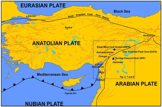
Figure 1.
Tectonic map of Anatolia distinguishing the involved tectonic plates and their boundaries, as well as the location of the study area, indicated by a rectangle.
The series of 1:500,000 geological maps produced by the General Directorate of Mineral Research and Exploration of Türkiye (MTA) for the EAFZ region reveal the presence of folds and faults affecting metamorphic, sedimentary, and volcanic rocks spanning different ages, from the Precambrian to the Upper Cretaceous. Overall, the predominant orientation of local tectonic structures tends to be parallel to the EAFZ, and they connect with the Cyprus Arc through the Gulf of Iskenderun. Active faults with various orientations are part of transcurrent, transpressional, and transtensional tectonic scenarios, as described in different segments of the EAFZ (e.g., [8]). Specifically, the EAFZ can be divided into two primary branches: the northern strand, consisting of the Sürgü-Misis Fault System (SMFS, approximately 350 km in length), oriented in an east–west direction; and the southern branch, which serves as the boundary between Anatolia and Arabia, known as the Main Strand. This transform fault, oriented approximately N060°E, extends from Karlıova to Antakya (approximately 580 km in length) and connects with the Cyprus Arc and the Dead Sea Fault Zone. Near Türkoğlu (Kahramanmaraş province), the tectonic structures of the Main Strand experience a sudden change in direction, which has important kinematic implications, as discussed below in this paper.
It is also important to point out the Nurdağı-Pazarcık Fault (NPF), also known as the Narlıdağ or Narlı Fault, located near the cities of Kahramanmaraş and Gaziantep and parallel to the Main Strand of the EAFZ. This fault, oriented NNE, is considered a splay fault of the EAFZ, where the first high-magnitude earthquakes occurred before being transferred to the EAFZ [23,33].
3. Methodology
3.1. Seismic Data and Catalog
The seismic data used in this study were obtained from the seismic catalog of the Earthquake Data Center System of Türkiye (TEDCS), available through the web portal of the Authority for the Management of Disasters and Emergencies (AFAD) [34] and subsequently relocated by Lomax (2023) [35]. Additionally, data from the Kandilli Observatory and Earthquake Research Institute [36] were used in this work, also relocated by Lomax (2023) [35]. The seismic record covers the period from 1 January 2023, to 31 May 2023, due to the notable improvement in the precision of location estimates by Lomax (2023) [35] during this period. The uncertainties in the X, Y, and Z coordinates of the earthquake locations were reduced to less than 2 km. For this purpose, two datasets were compared: first, raw data from a catalog of more than 35,000 earthquakes collected by AFAD [34], and, second, relocated and filtered data from Lomax [35], comprising more than 5500 seismic events.
The study area was delimited to the southeastern part of Türkiye, specifically in the central and southwestern zones of the EAFZ. It included the vicinity of the Sürgü-Misis Fault System (SMFS) and the Main Strand segments of Erkenek, Pazarcik, and Amanos (according to the terminology of Duman and Emre, 2013 [8]), until its disappearance offshore in the Mediterranean Sea, to the south of the Gulf of Iskenderun. The area of interest was delimited approximately by the following geographical coordinates: Lat: 35.0–39.0° N and Long: 35.0–40.0° E (Figure 2).
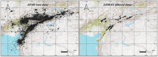
Figure 2.
Point cloud maps of the central and southwestern parts of the East Anatolian Fault Zone showing the locations of seismicity of the 2023 earthquake event in Türkiye–Syria. Left: Epicenters of the earthquakes from the AFAD dataset (raw); Right: epicenters from Lomax, 2023 [35] (relocated-filtered).
3.2. Use of Kernel Density Estimation for the Analysis of Seismicity
Geostatistics is a branch of statistics focused on the analysis and modeling of phenomena exhibiting spatial and/or temporal correlation. It deals with sets of variables where each value is associated with a specific position in space. In the context of interest, namely, seismology, the information about an earthquake is closely related to both the distance or position of its epicenter and the exact moment it occurred. Most geostatistical studies have focused on estimating expected values to create contour maps that correlate all variables of interest [37,38]. This approach can facilitate evaluations of resources (as in mining), the distribution of contaminants (in environmental sciences), or the development of seismic microzonation and mapping of seismic risk and perceived intensities for a given area in the event of an earthquake (in seismology). The objective of geostatistics in seismology is, therefore, to predict the possible spatial distribution of a seismological property. This process can be conducted manually or with the aid of computational tools, making it a powerful resource in various disciplines such as petroleum geology, hydrogeology, meteorology, ecology, and epidemiology. Given its widespread application, geostatistical methods have been integrated into geographic information systems, such as QGIS.
In this regard, the techniques specifically noted for their use in seismology are as follows:
- Geostatistical estimation approach. The most frequently used method is kriging, which predicts unknown values at unmeasured locations by utilizing the spatial correlation of known data points, based on a variogram model (e.g., [39,40,41]). Cokriging, which is an extension of kriging, simultaneously estimates multiple correlated variables (covariates) at unmeasured locations by incorporating information from secondary variables to improve the accuracy of estimates (e.g., [42]). And, based on the interpolation, inverse distance weighting (IDW) estimates unknown values at unmeasured locations by giving greater weight to nearby points based on the inverse of their distances (e.g., [43,44]).
- Machine learning methods are integrated with geostatistical methods to analyze and model spatial data, enhancing the prediction of spatial phenomena and improving resource estimation by using historical data and complex spatial relationships. A series of application examples in seismology are reviewed in [45]. The most known methods are the neural networking (e.g., [46,47]), logic or decision trees and random forest (e.g., [48,49,50]), and the support vector machine (SVM) (e.g., [51,52]).
- Density-based methods (e.g., [53,54]). These include point density analysis, which is a clustering algorithm that identifies groups (clusters) of closely packed points (events) based on their local density, enabling the detection of significant areas of activity while effectively handling noise and outliers. Kernel density estimation (KDE) methods estimate the probability density function of seismic events by placing a smooth kernel over each data point and adding them to create a continuous surface, allowing for the visualization of event concentrations and patterns without making strict assumptions about the data distribution.
- Less commonly used methods include stochastic simulation, probabilistic analysis, and spatial–temporal analysis (e.g., [55,56]).
All these techniques are complementary rather than mutually exclusive. Many of the cited studies have combined various methods depending on the desired analysis or applied hybrid methods combining them in phases to produce the maps.
There are numerous techniques applicable in seismology, but they differ significantly in terms of computational complexity, precision, flexibility, ease of interpretation, and response times. Estimation techniques, while offering high precision and ease of interpretation, tend to have low flexibility and long computation times, requiring large datasets and considerable processing. In contrast, machine learning methods, despite their high computational costs and complex results, provide high precision and flexibility. Density-based methods (e.g., KDE), on the other hand, appear to offer a balanced solution, with moderate computational costs, good precision, flexibility, and shorter response times, making them the most stable and convenient alternative. This is, therefore, the option presented in this paper.
Kernel density estimation (KDE) is a non-parametric method that allows defining a probability density function of a given random variable (e.g., [57]). In cases with insufficient information, or where it is impossible to assume the distribution shape (as with the spatial distribution of seismic events), a non-parametric estimation is commonly used. To accomplish this, techniques are used to estimate the distribution or relationship between variables without imposing a specific form (e.g., [58]). Among the techniques used in this work, kernel smoothing stands out, focused on the proximity and relationship among data points, such as the spatial location of earthquakes in a specific area. The kernel acts as a smoothing function placed on each data point, and its shape determines the contribution of that point to its neighborhood. The influence radius of each point, known as the bandwidth, can be defined according to the interest of the study. Combining all the contributions from each of the given points, an estimate of the probability density of a kernel is obtained.
The KDE method has been largely unused in seismology, but, nowadays, the increasing quality and density of seismic networks have made it more viable. This rise in the number of seismic catalogs allows for the application of such techniques in seismology due to the vast amount of recorded seismic events [59]. More common is the application of KDE techniques for generating seismic hazard maps (e.g., [60,61,62,63]). In the study area, this technique was used to generate maps to analyze the distribution of earthquakes with magnitudes greater than three [64], but there is no example of its application for increasing geological knowledge.
This paper proposes a new technique for geological and seismological analysis by applying the KDE method to the spatial distribution of seismic foci in any study area, previously grouped by different layers, related to seismogenic levels (Figure 3). By analyzing the relationship between the number of earthquakes and the depth of their hypocenters, different seismogenic layers can be identified.
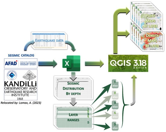
Figure 3.
Descriptive summary of the process to elaborate the maps. Flowchart to explain data processing. The initial data are from seismic data sources (including relocation by Lomax, 2023 [35]). These data are then processed with Microsoft Excel LTSC MSO (v. 16.0.1) to identify different layers (numbers 1 to 5) or seismogenic levels with depth. Finally, the different point clouds are processed with QGIS (v. 3.18) to obtain point clouds and kernel density maps for each seismic layer.
Regional seismicity data were analyzed to generate graphs representing the distribution of earthquakes as a function of depth and the frequency–magnitude distribution (Gutenberg–Richter law [65,66]). Those analyses allowed the identification of layers (represented by a relatively high frequency of earthquakes) with similar seismic behavior delimited by low seismicity zones. It is well known that seismic frequency varies with depth, and these variations can indicate changes in lithological composition, among other factors, and may be due to differences in the mechanical behavior of distinct levels of the lithosphere (crust and mantle).
Once the depth range of the different layers was delimited, an Excel file was obtained for each one containing all the relevant information, such as the earthquake coordinates, depth, and magnitude. The AFAD dataset [34], in which the focal depth is fixed or predetermined (typically around 7 km in this zone), was also included for comparison with the filtered point cloud (dataset of Lomax, 2023 [35]) and their effects on the interpretations. Fixed depths are commonly used in seismic catalogs to expedite the calculation processes for certain parameters but can lead to misinterpretation of geological and seismological data. Evaluating these effects and whether this new technique helped to minimize them were also addressed in this work.
The next step was to process the information of each seismic layer through appropriate software that allows kernel analysis, QGIS (v. 3.18) in this case. Once the Excel files were imported into QGIS, they were converted to a shapefile format for their processing. Heatmaps or KDE maps can be created using a specific kernel method. In statistical analysis, as it was mentioned previously, the term kernel refers to a window function that sets a radius of influence around a given position for the measured parameter. When an element falls within that radius, its value is defined by a specific function, while for those outside this radius, its value is zero. The bandwidth must be specified and expressed in meters, degrees, or map units in QGIS. In this study, considering the size of the working area, a bandwidth of 0.05° was used. To achieve higher resolution, a pixel size of 0.001° was selected.
The choice of a 0.05° bandwidth was determined based on the study area, which covered approximately 250,000 km2, resulting in a buffering influence area of 34.90 km2, along with the spatial distribution of more than 5500 recorded seismic events. This value provided an optimal balance between spatial detail and the smoothing necessary to capture coherent seismic patterns in such an extensive region. A smaller bandwidth would be good for smaller study areas or a greater number of seismic events. For the parameters in this study, a smaller bandwidth would have increased the local resolution but introduced noise in areas with lower event density. Conversely, a larger bandwidth would have excessively smoothed the seismic distribution patterns, reducing the ability to identify key geological structures. Therefore, the 0.05° value enabled capturing both the global trends and regional details of seismicity in the study area. Figure 4 illustrates the effect of bandwidth on the resulting kernel maps.
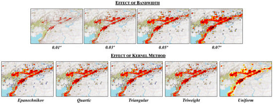
Figure 4.
Evaluation of the impact on seismic density distribution due to changes in bandwidth (upper part of the figure) and the kernel method employed (lower part of the figure). As shown, lower bandwidth values generate more detailed results but introduce greater noise, while higher values emphasize regional patterns at the expense of local details. The kernel method determines the influence of a value on its surroundings, as illustrated by the functions shown in Figure 5. The choice of kernel function shows minimal differences (except for the uniform method) compared to the impact of bandwidth variations.
Also, a weighting function for the determination of the parameter value should be chosen. A quartic kernel function, K(x), was employed. This quartic method is based on the fourth-degree polynomial [67]:
where x is the bounded support, closely related to the bandwidth, always within a value between −1 and 1. The function is 0 for values of x outside the support.
In QGIS, several kernel functions are available by default, including quartic, triweight, uniform, Epanechnikov, and triangular functions. All these kernel functions (and other examples) are illustrated in Figure 5. For this study, the quartic function was selected due to its ability to provide an optimal balance between smoothing and spatial accuracy. Unlike the triweight function, which decreases more rapidly towards the edges, the quartic function offers a smoother transition, allowing for better detection of heterogeneously distributed patterns. The uniform function, by assigning equal weight to all points within the bandwidth, is not suitable for capturing the gradual variation in data. In contrast, the Epanechnikov function provides similar smoothing to the quartic function but has a reduced ability to detect subtle variations. Finally, the triangular function tends to overly prioritize nearby points, which could exclude the influence of distant yet relevant seismic events. Thus, the quartic function ensures an optimal balance in seismic density analysis, highlighting values closer to the center while maintaining smoother behavior than other kernel functions, such as the triweight function, which decays more rapidly towards the edges. However, it is important to note that the differences between kernel functions are minimal compared to the significant impact that bandwidth variations have on the results (see Figure 4).
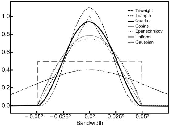
Figure 5.
Examples of kernel functions. The geometry of the graphs corresponding to various kernel functions K(x) illustrates the influence of the data on their surroundings (taking values between 0 and 1 on the vertical axis) versus the radius of influence (horizontal axis), expressed in degrees. All curves are normalized to the same unit area.
Finally, color delineation based on quartiles is established. The first quartile is represented in blue (indicating higher data dispersion), the second in yellow, the third in red, and the fourth in black (indicating the nuclei of high seismic density). Since the range is continuous, there may be intermediate color combinations resulting from the blending of these primary colors.
3.3. Profiles Along the EAFZ
Two profiles were made along the studied fault trace (Main Strand of the EAFZ, approximately oriented N060°E) showing the depth distribution of the hypocenters of the recorded earthquakes: one for raw data and one for relocated-filtered data. QGIS was used to establish influence radii for the points considered in the profiles. Most of the earthquakes associated with the main fault system were identified within a distance that never exceeded 20 km from the trace of the main fault (e.g., [5,68]). Therefore, a buffer with a radius of 0.2° was selected, considering the data points included within that influence radius and excluding those outside it. Additionally, the kernel quartic method with a bandwidth of 2 (in units of the map, which was equivalent to a bandwidth of around 1 km, an area of influence of around 3 km2) was used for this specific case, due to the dimension and scale of the profiles, with a total area of 15,000 km2. Note that the relationship between the total surface and the area of influence of the kernel quartic method was of the same order of magnitude in profiles and maps.
4. Results and Interpretations
4.1. Seismic Distribution by Depth and Delimited Layers
The analysis of the distribution of seismicity with depth allows the identification of the layers that exhibit differentiated seismic behavior. These layers were defined by the main trend and delimited, as described previously, by low-seismicity zones represented by minima in the seismic frequency. Figure 6 compares the distribution of the seismicity with depth for the two datasets (AFAD [34] and Lomax, 2023 [35]). The gray range in both cases represents the limits of the point cloud, which includes all the data recorded. The seismicity in the area shows the typical distribution, with most earthquakes concentrated in the shallower layers and progressively decreasing with depth (see also, e.g., [68,69,70]). Seismicity is practically absent in the lower part of the lithosphere; in both cases, there is virtually no seismicity below 20 km (only a few very isolated hypocenters). Likewise, four minima in earthquake concentration are recognized, located at depths of 4.9, 8.8, 14.5, and 18.7 km for the AFAD data (raw data) and at depths of 4.8, 7.9, 14.9, and 18.9 km for the filtered data of Lomax (2023) [35]. These minima indicate the presence of zones of lower seismicity and, therefore, constitute contacts between layers with distinct mechanical behavior. Filtered data processing estimated a hypocentral error of less than 2 km, but the minima in the raw data are included within a ±1 km range (orange band, Figure 6) from the minima in the filtered data. Thus, the raw and filtered data minima align very well, indicating that both datasets recognize the same minima (and maxima) within a relatively small error range.
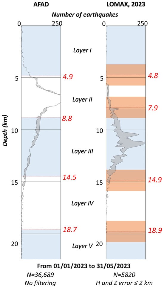
Figure 6.
Comparison of the depth distribution of seismicity (number of earthquakes vs. depth). Left: Non-filtered data from the Disaster and Emergency Management Authority (AFAD) dataset. Right: Relocated and filtered data from Lomax (2023) [35]. Layers separated by zones with minimum earthquake frequency are highlighted in alternating blue and white bands (Layers I–V). For raw data: Layer I (0.0–4.9 km), Layer II (4.9–8.8 km), Layer III (8.8–14.5 km), Layer IV (14.5–18.7 km), and Layer V (below 18.7 km). For filtered data: Layer I (0.0–4.8 km), Layer II (4.8–7.9 km), Layer III (7.9–14.9 km), Layer IV (14.9–18.9 km), and Layer V (below 18.9 km). An orange ±1 km range (less than the uncertainty in the location, ±2 km, by Lomax, 2023 [35]) is used to illustrate the statistical concordance of the layers observed in both datasets.
Areas with high seismic recurrence indicate zones of interest for studying and recognizing brittle seismogenic structures. The seismicity density within the seismically active layers does not exactly coincide between the two datasets, with the absolute maximum occurring at an approximately 7 km depth in the raw data (AFAD) and around an 11 km depth in the filtered data (Lomax [35]). As described earlier, 7 km is the predetermined depth for data processing in AFAD [34] and could account for this maximum. However, the filtered data also show a minor peak at an approximately 8 km depth. In this case, the raw data display a smaller peak coinciding with the maximum observed in the filtered data. Although 7 km is a predefined depth for calculations, the observed correlation with the filtered data suggests the presence of a genuine seismically active layer around this depth.
In this way, five layers were distinguished: In the case of raw data: Layer I, from 0.0 to 4.9 km; Layer II, from 4.9 to 8.8 km; Layer III, from 8.8 to 14.5 km; Layer IV, from 14.5 to 18.7 km; and Layer V, including the deeper data points below 18.7 km. In the case of filtered data: Layer I, from 0.0 to 4.8 km; Layer II, from 4.8 to 7.9 km; Layer III, from 7.9 to 14.9 km; Layer IV, from 14.9 to 18.9 km; and finally, Layer V, below 18.9 km.
Although the differences between the depths of the boundaries of the layers defined by raw (AFAD) and filtered (Lomax [35]) data are smaller than the error in determining the depth of the earthquakes—up to 2 km for the filtered data—there is a significant variation in the density of earthquakes for each layer in both datasets, as indicated above (Figure 6), which are analyzed in more detail below.
4.2. Point Clouds by Layer
All registered data points are represented in Figure 2, showing the distribution of earthquake foci over a digital terrain model. As can be seen, the dispersion of the data is greater in the case of raw data, as expected, but they show a more continuous trace than the filtered data. However, the main morphology of the point clouds shows the same tendency for both datasets. In both cases, the point lineations coincide with the traces of the Main Strand of the EAFZ and the SMFS. The nuclei of historically high frequencies of earthquakes, where recent events also generate more aftershocks and larger magnitudes, were recognized in both datasets. These maps show that most of the seismicity is concentrated in the northwest of the study area (over the Anatolian plate) and is virtually absent in the southeast (over the Arabian plate).
Point cloud maps are also represented for each layer (I to V) identified previously. A comparison of these maps is shown in Figure 7. Although the difference in the number of data points between the two datasets varies by an order of magnitude, the patterns are consistent. In both cases, the data points are concentrated in the upper layers, and their number decreases progressively in the lower layers. Seismicity is very scarce, virtually absent, at depths greater than 18.9 km for filtered data and 18.7 km for raw data. The unfiltered data show the non-existent connection between the MSFZ and the Main Strand of the EAFZ in most layers (maybe except in Layer II), whereas the filtered data suggest this same interpretation but less clearly. The 3D configuration of the data points may describe the morphology of the boundary between the Arabian and Anatolian plates. The analysis of the 3D disposition of the maps in both cases reveals that earthquakes are consistently distributed along the traces of the EAFZ and SMFS, describing structures with significant verticality from the surface downward.
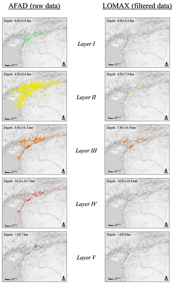
Figure 7.
Comparison of point cloud maps for the central and southwestern parts of the EAFZ, represented at different depth ranges (seismological layers) identified by the seismic distribution profile, Layers I to V (Figure 5). Left: AFAD (raw data). Right: Lomax, 2023 [35] (relocated-filtered data). Each color was selected to facilitate comparison and to represent the increasing depth (shallower in green and greater depths in black). The figures present scatter plots of seismic points, which display the raw locations of seismic events without any statistical treatment. A stacked view of the maps is shown in Appendix A (Figure A1).
4.3. Kernel Density Maps by Layer
Kernel maps were generated for each layer (Figure 8), applying the process described in the Methodology Section. This statistical approach allowed for analyzing the density of the seismic events over the defined area. This method smooths the data, highlighting regions with higher concentrations of seismic activity and providing a more informative representation of the underlying patterns. The black (or red) nuclei, representing higher-frequency zones of points, show a very similar tendency in both datasets (note the ‘number 7’-like form of the density nuclei). As observed in the point cloud maps, the raw data exhibit a more continuous trace, whereas the filtered data only show discontinuous nuclei aligned along the Main Strand of the EAFZ and MSFZ. Similarly, the data points appear to concentrate approximately along the trace of the faults in the outer layers, converging at deeper layers into narrower high-density nuclei. This pattern is more evident in the raw data, with surface nuclei being more extensive (e.g., in Layer II) relative to the more concentrated nuclei at depth (Layers III to V). The black nuclei in Layer II of the raw data exhibit similar forms to the kernel density map of Layer II for filtered data, also aligned with the fault traces recognized at the surface. It can be suggested that the kernel maps reproduce a similar filtering function as the relocation of data points.
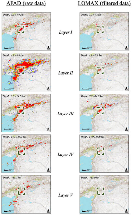
Figure 8.
Comparison of kernel density maps of seismicity density for the central and southwestern parts of the East Anatolian Fault Zone (EAFZ), represented at different depth ranges (seismological layers) identified by the seismic distribution profile, Layers I to V (Figure 5). Left: AFAD (raw data). Right: Lomax, 2023 [35] (relocated-filtered data). It illustrates the same seismic data from Figure 6 but applying KDE, a statistical approach, to highlight the patterns and greater frequency of earthquakes (in black). The area where the converging nuclei from upper to lower layers are easily identifiable is highlighted by a rectangle. This is approximately the same area used to create the detailed map in Figure 9. A stacked view of the maps is shown in Appendix A (Figure A2).
The main difference between the datasets can be observed in the southwest of the study area: while the raw data show a relatively high concentration of data at depth (Layers III to V), probably resulting from the interaction of the EAFZ with the subduction in the Cyprus arc, the filtered data have no recorded points in this region. The raw data allow for a more complete delineation of the plate boundaries.
The kernel density maps allow for the clear definition of a disconnection between the density nuclei belonging to the Main Strand of the EAFZ and those that are part of the SMFS. In this regard, density maps enable the delimitation of different segments within the fault zone.
By examining the maps in more detail, the area where the first major earthquakes in Türkiye occurred (highlighted with dashed rectangles in Figure 8), both maps (AFAD: raw data and Lomax, 2023 [35]: filtered data) reveal that the density cores in the upper layers correspond to the Main Strand of the EAFZ and the NPF traces. These two cores converge at depth into a single elongated nucleus parallel to the direction of the EAFZ. This three-dimensional geometry of the seismicity distribution suggests large, elongated funnels resembling fan or palm-tree structures in two-dimensional sections.
4.4. Seismicity Profiles
The seismicity profiles along the EAFZ are presented in Figure 9. The profiles in the center of the figure show the magnitude of the earthquakes, while the profiles at the bottom use the kernel density method. As described earlier, seismicity in the southwest of the study area is not represented in the filtered data due to the extremely rigorous filtering process. Four black nuclei are recognized in the raw data, three of which coincide in the horizontal coordinate with the high-density nuclei shown in the filtered data. Seismicity is distributed up to a depth of around 20 km along the transect. Particularly in the raw data, it can be observed that below this depth, the deeper foci are located approximately above the vertical of the kernel maxima. The greatest-magnitude earthquakes coincide with the high-density cores in both datasets, despite some of these earthquakes not being included in the filtered data.
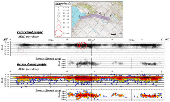
Figure 9.
Seismicity profiles along the Main Strand of the EAFZ oriented approximately N60°E. Upper image: The location of the profile and the buffer used to select the seismic foci. Center of the figure: Point cloud of earthquakes at different depths, differentiated by magnitude. Upper: Raw data (AFAD); Lower: filtered data (Lomax, 2023 [35]). At the bottom of the figure: Kernel density profiles. Upper: Raw data; Lower: filtered data. Different points are marked with letters both on the profiles and on the map to accurately locate the black loci.
The major limitation observed in the raw data profile is the notable elongated structure at a depth of 7 km due to the fixed depth of the data. However, this does not prevent the identification of the true morphology of the nuclei.
5. Discussion
5.1. Seismicity and Geology of the EAFZ
A close correlation between the point clouds from both datasets and the geological characteristics of the study area is evident (Figure 10). All data points are directly associated with both the Main Strand and the SMFS of the EAFZ, aligning parallel to specific geological formations. In the southwestern part of the Main Strand, the epicenter point clouds are concentrated over Quaternary deposits and ophiolites. This ophiolitic boundary between Anatolia and Arabia is distinctly delineated by the earthquakes that occurred during the February 2023 event. On the other hand, in the SMFS, point clouds tend to align predominantly with the boundaries of elongated blocks made up of metamorphic rocks of various ages, ranging from Precambrian to Cretaceous. It is worth noting that, despite the proximity to active faults, virtually no seismic activity is recorded in the volcanic and sedimentary rock formations of the Paleozoic era, both to the north and south of the study area, as well as in the plutonic formations located in the northeast.
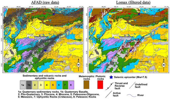
Figure 10.
Detailed geological map of the surroundings of the major earthquakes, with epicenters from both datasets: AFAD (raw dataset, black dots) on the left and Lomax (2023) [35] (relocated-filtered, red dots) on the right.
It is intriguing to note that despite the historical susceptibility of the city of Malatya to earthquakes, there was no increase in seismic activity in its vicinity during the February 2023 event. This phenomenon may be attributed to a decoupling effect along the EAFZ to the northeast and southwest of Malatya (SMFS and Main Strand of the EAFZ, respectively), as also shown by the kernel density maps (Figure 8).
The distribution of seismicity at depth appears to indicate the presence of extensive highly dipping to subvertical fractures converging at depth along the trace of the EAFZ (e.g., [69]). While at the surface, the structure spans a relatively broad area, at depths exceeding 15 km, all epicenters are located along a distinct single fault or core of high seismicity (see also, e.g., [69,70]). Güvercin et al. (2022) [6] deduced a dip towards the N for this high-seismicity core between at least, 7 and 20 km deep. This palm-shaped arrangement (Figure 8) that extends towards the surface distinctly resembles the structures observed in smaller-scale strike–slip faults in various regions around the world (e.g., [71,72]).
5.2. Evaluation of the Method and Comparison of AFAD and Lomax Datasets Maps
This new method allows for the comparison of the seismic distribution graphs of the two datasets (AFAD [34] and Lomax, 2023 [35]). The depth distribution of seismicity shows similar behavior, with most earthquakes occurring in shallower layers and decreasing in frequency at greater depths. The seismicity in both cases is scarce and virtually non-existent below 20 km. This distribution coincides with that observed in other transform fault contexts, such as the San Andreas Fault, where seismicity is effectively absent below 23 km [73,74]. The upper layers accommodate deformation by activating fault structures that concentrate all the seismicity, while below 20 km, this deformation might occur by non-seismogenic creep.
The recognition of minima in earthquake concentration, which indicate lower seismicity zones and changes in the mechanical behavior of materials, also allows for the definition of the five layers related to the seismogenic levels that coincide in both data sources within a ±1 km range. Filtered data processing estimated a hypocentral error of less than 2 km, but the minima in the raw data fall within a narrower range. The strong agreement between the two catalogs—raw and relocated data—in the depth distribution of seismicity, despite this being the variable with the highest uncertainty in the calculations of seismic parameters, fosters optimism regarding the interpretations derived from the maps.
According to the kernel maps generated for the two datasets, both show similar high-frequency zones with a distinctive ‘number 7’-like shape in plan view. This form aligns well with the trace of the Main Strand of the EAFZ and SMFS activated during this seismological event. The raw data display a more continuous density pattern, while the filtered data show discontinuous high-density nuclei. However, the KDE maps of the Lomax (2023) [35] dataset are consistent with the black nuclei observed in the AFAD data. In both cases, the kernel maps reveal 3D seismically active structures that resemble large, elongated funnels or palm-tree formations. This method enables the characterization of the three-dimensional architecture of large-scale structures, which are comparable with the geometry of smaller-scale structures observed in other regions, as described previously. Additionally, the seismicity profiles along the Main Strand of the EAFZ show significant agreement between the two datasets, indicating large vertical structures that converge at the vertical of the black nuclei. These structures are consistent with the interpretations derived from the kernel maps.
Concerning advantages and disadvantages, unfiltered data allow for quick access and processing. They facilitate the analysis of a larger volume of data, providing a more comprehensive view of seismic activity, including smaller earthquakes that might be lost after filtering. Additionally, the data have lower processing costs and are easier to automate, enabling the application of statistical analyses and subsequent filtering.
On the other hand, the cons include high uncertainty in both the location and magnitude of events, a higher presence of noise and anomalies due to erroneous data that require additional cleaning and filtering, and a greater difficulty in identifying patterns, critical zones, or trends due to the higher dispersion of the data. However, all these issues can be minimized through an effective filtering process (as, for example, KDE does).
In contrast, relocated data ensure higher precision and reliability, as well as a significant reduction in noise due to rigorous cleaning, and allow for the accurate identification of patterns, even migration, fault activity, and risk zones, with great confidence.
However, the data require a long processing time (ranging from days to months) to produce a catalog with fewer earthquakes, are more difficult to automate, frequently need human intervention for calculation, cannot be obtained in real time, and potentially exclude relevant events (such as precursors or aftershocks) either due to filtering or because their magnitudes fall below the threshold required for precise calculation.
This technique must be applied considering a series of assumptions and limitations:
- Fundamentals and limitations of the kernel technique: One of the primary limitations of all KDE methods is that they produce an image-based representation of seismic data, which requires expert interpretation. Another limitation of this new technique is the determination of the depth range of the layers based on the seismicity distribution, which should ideally be performed by an expert.
- Regarding scale, data volume, type of kernel method, and bandwidth, a large amount of seismic data is required, and the bandwidth must be selected based on this data volume and the scale of the study area. Larger areas or lower data volumes necessitate greater bandwidths. Additionally, the kernel method should be chosen according to the study’s objectives, but, generally, kernel methods that emphasize values closer together are preferable.
Despite all of these limitations, this new technique is useful and should be considered in future studies according to the next contexts:
- Theoretical frameworks: This method could be applied in numerous contexts, such as fracture theory, which models the distribution of seismic events concerning geological faults and fracture structures. It can also be utilized in fault instability theory to evaluate patterns that may predict future fault behavior and in seismic risk assessment models to identify areas with high densities of seismic occurrences. Additionally, it aids in spatial analysis in geology by examining the distribution of geological features and their relationship with seismic activity. This technique is beneficial in fluid dynamics within faults, as it helps visualize how fluid pressure correlates with seismic events. Moreover, it can be applied in plate tectonics theory to analyze the interaction between tectonic processes and seismic activity, as well as in wave propagation models and studies of seismic precursors. Of course, this innovative technique can be utilized across various depth layers recognized in any planetary area.
- Geological contexts: This method was applied in complex environments, such as this major transform boundary (Anatolian-Arabian plate boundary), but it can also be utilized in various other settings, including subduction zones, mid-ocean ridges, or volcanic areas.
To summarize, both the filtered dataset and the unfiltered dataset led to similar interpretations when the KDE method was applied. Since the uncertainty in earthquake locations is usually random, a high concentration of earthquakes determined from non-relocated data should be found in a position close to the nucleus identified from the relocated data, which is what was observed in the case analyzed in this work. The KDE functions proved to be useful treatments and can be considered as a sort of initial, graphical, fast relocation process, accelerating both the treatment and interpretation of data. This approach enhances geological and seismological knowledge and improves earthquake preparedness, prevention, coordination, and rapid response.
6. Conclusions
Two populations of seismic foci point clouds from the seismic series that occurred in Türkiye and Syria during 2023, containing over 60,000 events, were analyzed. The datasets included raw data recorded by the Turkish Disaster and Emergency Management Authority (AFAD) [34] and relocated and filtered data from Lomax (2023) [35]. A new technique was employed to compare these datasets. Analyzing the seismic distribution with depth allowed for the identification of minimal-frequency earthquake levels that separate distinct seismically active layers associated with the mechanical behavior of the materials.
This new technique allows the differentiation of seismogenic levels on which the kernel is applied to recognize the geometry of deep three-dimensional structures. Five seismic layers were defined for both raw and filtered data, with slight variations in depth boundaries: for the raw data: Layer I (0.0–4.9 km), Layer II (4.9–8.8 km), Layer III (8.8–14.5 km), Layer IV (14.5–18.7 km), and Layer V (below 18.7 km); for filtered data: Layer I (0.0–4.8 km), Layer II (4.8–7.9 km), Layer III (7.9–14.9 km), Layer IV (14.9–18.9 km), and Layer V (below 18.9 km).
Both datasets align closely with the Main Strand of the EAFZ and the SMFS, with high-frequency earthquake nuclei recognized in both. The raw data suggest a lack of connection between SMFS and the Main Strand of the EAFZ in most layers.
Kernel density analysis demonstrated that both datasets yield similar geological interpretations. In the southwestern Main Strand, epicenters are concentrated over Quaternary deposits and ophiolites, marked by the February 2023 earthquakes. In contrast, the SMFS aligns with the boundaries of elongated metamorphic blocks from the Precambrian to the Cretaceous. Despite proximity to active faults, seismic activity is notably absent in Paleozoic volcanic and sedimentary formations and northeastern plutonic formations.
The seismicity at depth reveals extensive, highly dipping to subvertical fractures converging along the EAFZ. While surface structures span a broad area, deeper seismicity is concentrated along a distinct fault core. This core, dipping northward between a 7 and 20 km depth, resembles the palm-shaped structures seen in strike-slip faults globally.
Seismicity profiles reveal four high-density nuclei for raw data, with three of them coinciding in horizontal coordinates with those of filtered data. Seismicity is observed up to about a 20 km depth, with high-magnitude earthquakes corresponding to density cores in both datasets. Despite limitations like the 7 km depth structure in the raw data (an artifact due to routine depth attribution of the used catalog of non-relocated data), the profiles effectively highlight the true morphology of seismicity distribution.
Overall, this study demonstrates that a comprehensive seismic catalog with significantly higher uncertainty (such as AFAD database) yields similar interpretations when analyzed using KDE compared to a relocated catalog (such as the Lomax database). This proves to be an effective tool for rapid seismic data treatment, a certain degree of filtering is inherently achieved using KDE (simulating relocation), and interpretation. It would be ideal to work with these relocated data with very high precision and reliability whenever available, but this is not always possible. While relocated catalogs are ideal for more precise and well-defined studies, unfiltered data can lead to similar interpretations with a significantly shorter response time. While the first type of catalog can be processed almost instantly or within a few hours after the earthquake occurs, the second type requires a more extensive effort and longer processing times (days or even months). This technique, despite its limitations, provides more information relative to other methods in a short time. It can help to better define a three-dimensional seismic hazards, critical zones, segment faults, and segments that have been active but are currently inactive.
To evaluate the accuracy of the interpretations resulting from the analysis of the unfiltered catalog, this study included two forms of validation: an internal validation, which was performed by comparing two populations, one of which has high reliability and certainty (Section 5.2); and an external validation, achieved through coherence with regional geological knowledge (Section 5.1). Based on these validations and the low deviation from the optimal (represented by the control population), it is concluded that the procedure is valid for comparing these two populations, which is further corroborated by its alignment with independent sources, such as geological data. Moreover, the results are fully supported by additional sources, such as geomorphology or geophysics, which also converge on the same observations.
To conclude, this method enhances geological and seismological understanding, thereby contributing to improved earthquake preparedness and response in the event of a major earthquake. We propose that this technique could be a routine method used in seismic centers due to its versatility, agility, and ease of use. This technique, combined with a tectonic and rheological study of any portion of the lithosphere, is key for defining the different seismotectonic levels in that zone. This could lead to the generation of a catalog of slices or layers for each section of the Earth, like how we currently perform seismic zoning for crustal resistance in plan view, but now vertically within the lithosphere.
Author Contributions
Conceptualization, D.A.L., F.M.A.-C. and C.F.; methodology: D.A.L., F.M.A.-C. and C.F.; software: D.A.L.; validation: D.A.L., F.M.A.-C. and C.F.; formal analysis: D.A.L., F.M.A.-C. and C.F.; investigation: D.A.L., F.M.A.-C. and C.F.; resources: D.A.L., F.M.A.-C. and C.F.; data curation: D.A.L.; writing—original draft preparation: D.A.L., F.M.A.-C. and C.F.; visualization: D.A.L.; supervision: F.M.A.-C. and C.F.; project administration: F.M.A.-C. and C.F.; funding acquisition: F.M.A.-C. and C.F. All authors have read and agreed to the published version of the manuscript.
Funding
The authors acknowledge the funding provided by the Research and Transfer Policy Strategy (EPIT) of the University of Huelva through the predoctoral contract for the promotion of hiring early-career researchers (EPIT20/00832), which enabled David Amador Luna to carry out his research, the results of which are reflected in this publication.
Data Availability Statement
The seismic data used in this study were obtained from the seismic catalog of the Earthquake Data Center System of Türkiye (TEDCS), available through the web portal of the Authority for the Management of Disasters and Emergencies (AFAD) and subsequently relocated by Lomax (2023) [35]. Additionally, data from the Kandilli Observatory and Earthquake Research Institute were used in this work, also relocated by Lomax (2023) [35]. The reference and links are listed below: AFAD (Disaster and Emergency Management Authority of Turkey). National Seismic Network of Türkiye (DDA). International Federation of Digital Seismograph Networks 2024. https://tdvm.afad.gov.tr/ accessed on 27 May 2024; Lomax, A. Precise, NLL-SSST-coherence hypocenter catalog for the 2023 Mw 7.8 and Mw 7.6 SE Turkey earthquake sequence. 2023. https://doi.org/10.5281/zenodo.7699882; KOERI. Kandilli Observatory and Earthquake Research Institute (KOERI)–Istanbul, Turkey 2024. Retrieved from http://www.koeri.boun.edu.tr/ accessed on 27 May 2024.
Acknowledgments
We would like to thank the AFAD and KOERI organizations for their efforts in collecting all the seismic records. David Amador Luna acknowledges the funding from the ‘Estrategia Política de Investigación y Transferencia’ (EPIT) of the University of Huelva for the predoctoral contract to promote the hiring of novice research personnel (EPIT20/00832), without which this work would not have been possible. We warmly acknowledge the comments of the three anonymous reviewers that have substantially aided to improve the original manuscript. We also want to thank Elisa Buforn for her guidance in comparing both catalogs and advising on the hypocenter errors to consider.
Conflicts of Interest
The authors declare no conflicts of interest.
Appendix A
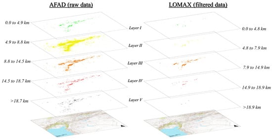
Figure A1.
Comparison of stacked point cloud maps for the central and southwestern part of the EAFZ, represented at different depth ranges (seismological layers) identified by the seismic distribution profile, Layers I to V (Figure 5). Left: AFAD (raw data). Right: Lomax, 2023 [35] (relocated-filtered data). This figure represents the same maps as in Figure 7 but stacked to illustrate the 3D morphology of the patterns. For color codes see Figure 7.
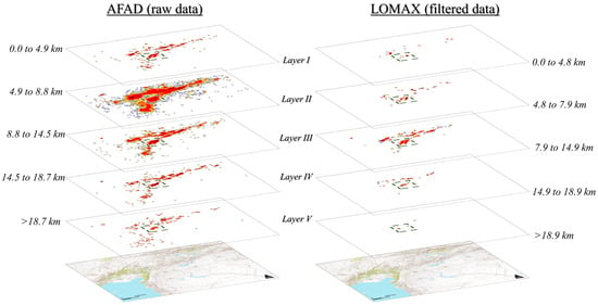
Figure A2.
Comparison of stacked kernel maps of seismicity density for the central and southwestern part of the East Anatolian Fault Zone (EAFZ), represented at different depth ranges (seismological layers) identified by the seismic distribution profile, Layers I to V (Figure 5). Left: AFAD (raw data). Right: Lomax, 2023 [35] (relocated-filtered data). The area where the converging nuclei from upper to lower layers is easily identifiable is highlighted by a rectangle. This figure represents the same maps as in Figure 8 but stacked to illustrate the 3D morphology of the patterns. For color codes see Figure 8.
References
- Allen, C.R. Active Faulting in Northern Turkey; Rep. 1577; Division of Geological Sciences, California Institute of Technology: Pasadena, CA, USA, 1969; 32p. [Google Scholar]
- Arpat, E.; Şaroğlu, F. The East Anatolian Fault system; thoughts on its development. Bull. Miner. Res. Explor. Inst. Turk. 1972, 78, 33–39. [Google Scholar]
- Şaroğlu, F.; Emre, Ö.; Kusçu, I. Active Fault Map of Turkey; General Directorate of Mineral Research and Exploration: Ankara, Turkey, 1992. [Google Scholar]
- Westaway, R.; Arger, J. Kinematics of the Malatya–Ovacık Fault Zone. Geodin. Acta 2001, 14, 103–131. [Google Scholar] [CrossRef]
- Türkoğlu, E.; Unsworth, M.; Bulut, F.; Çağlar, İ. Crustal structure of the North Anatolian and East Anatolian Fault Systems from magnetotelluric data. Phys. Earth Planet. Inter. 2015, 241, 1–14. [Google Scholar] [CrossRef]
- Güvercin, S.E.; Karabulut, H.; Konca, A.Ö.; Doğan, U.; Ergintav, S. Active seismotectonics of the East Anatolian Fault. Geophys. J. Int. 2022, 230, 50–69. [Google Scholar] [CrossRef]
- Barka, A.A.; Kadinsky-Cade, K. Strike-slip fault geometry in Turkey and its influence on earthquake activity. Tectonics 1988, 7, 663–684. [Google Scholar] [CrossRef]
- Duman, T.Y.; Emre, Ö. The East Anatolian Fault: Geometry, Segmentation and Jog Characteristics. Geol. Soc. Lond. Spec. Publ. 2013, 372, 495–529. [Google Scholar] [CrossRef]
- Bletery, Q.; Cavalié, O.; Nocquet, J.M.; Ragon, T. Distribution of interseismic coupling along the north and east Anatolian faults inferred from InSAR and GPS data. Geophys. Res. Lett. 2020, 47, e2020GL087775. [Google Scholar] [CrossRef]
- Över, S.; Özden, S.; Yilmaz, H. Late Cenozoic stress evolution along the Karasu Valley, SE Turkey. Tectonophysics 2004, 380, 43–68. [Google Scholar] [CrossRef]
- Över, S.; Özden, S.; Unlugenc, U.C.; Yilmaz, H. A synthesis: Late Cenozoic stress field distribution at northeastern corner of the Eastern Mediterranean, SE Turkey. Comptes Rendus Geosci. 2004, 336, 93–103. [Google Scholar] [CrossRef]
- Yilmaz, H.; Över, S.; Özden, S. Kinematics of the East Anatolian Fault Zone between Turkoglu (Kahramanmaras) and Celikhan (Adiyaman), eastern Turkey. Earth Planets Space 2006, 58, 1463–1473. [Google Scholar] [CrossRef]
- Aksoy, E.; İnceöz, M.; Koçyığıt, A. Lake Hazar Basin: A negative flower structure on the East Anatolian Fault System (EAFS), SE Turkey. Turk. J. Earth Sci. 2007, 16, 319–338. [Google Scholar]
- Köküm, M.; İnceöz, M. Structural analysis of the northern part of the East Anatolian Fault System. J. Struct. Geol. 2018, 114, 55–63. [Google Scholar] [CrossRef]
- Yönlü, O.; Altunel, E.; Karabacak, V. Geological and geomorphological evidence for the southwestern extension of the East Anatolian Fault Zone, Turkey. Earth Planet. Sci. Lett. 2017, 469, 1–14. [Google Scholar] [CrossRef]
- Aktug, B.; Ozener, H.; Dogru, A.; Sabuncu, A.; Turgut, B.; Halicioglu, K.; Yilmaz, O.; Havazli, E. Slip rates and seismic potential on the East Anatolian Fault System using an improved GPS velocity field. J. Geodyn. 2016, 94–95, 1–12. [Google Scholar] [CrossRef]
- Özkan, A.; Yavaşoğlu, H.H.; Masson, F. Present-day strain accumulations and fault kinematics at the Hatay Triple Junction using new geodetic constraints. Tectonophysics 2023, 854, 229819. [Google Scholar] [CrossRef]
- Akin, U. Investigation of the seismic velocity distribution and crustal structure of Turkey by means of gravity data. Bull. Miner. Res. Explor. 2016, 153, 185–202. [Google Scholar]
- Abgarmi, B.; Delph, J.R.; Ozacar, A.; Beck, S.L.; Zandt, G.; Sandvol, E.; Turkelli, N.; Biryol, C.B. Structure of the crust and African slab beneath the central Anatolia plateau from receiver functions: New insights on isostatic compensation and slab dynamics. Geosphere 2017, 13, 1774–1787. [Google Scholar] [CrossRef]
- Ozer, C.; Ozyazicioglu, M.; Gok, E.; Polat, O. Imaging the crustal structure throughout the East Anatolian Fault Zone, Turkey, by local earthquake tomography. Pure Appl. Geophys. 2019, 176, 2235–2261. [Google Scholar] [CrossRef]
- Artemieva, I.; Shulgin, A. Geodynamics of Anatolia: Lithosphere thermal structure and thickness. Tectonics 2019, 38, 4465–4487. [Google Scholar] [CrossRef]
- Delouis, B.; van den Ende, M.; Ampuero, J.P. Kinematic rupture model of the February 6th 2023 Mw7.8 Turkey earthquake from a large set of near-source strong-motion records combined with GNSS offsets reveals intermittent supershear rupture. Bull. Geol. Soc. Am. 2024, 114, 726–740. [Google Scholar] [CrossRef]
- Okuwaki, R.; Yagi, Y.; Taymaz, T.; Hicks, S.P. Multi-scale rupture growth with alternating directions in a complex fault network during the 2023 south-eastern Türkiye and Syria earthquake doublet. Geophys. Res. Lett. 2023, 50, e2023GL103480. [Google Scholar] [CrossRef]
- McKenzie, D. Active tectonics of the Mediterranean region. Geophys. J. Int. 1972, 30, 109–185. [Google Scholar] [CrossRef]
- Dewey, J.F.; Pitman, W.C.; Ryan, W.B.F.; Bonnin, J. Plate tectonics and the evolution of the Alpine system. Geol. Soc. Am. Bull. 1973, 84, 3137–3180. [Google Scholar] [CrossRef]
- Stampfli, G.M. Tethyan oceans. Geol. Soc. Lond. Spec. Publ. 2000, 173, 1–23. [Google Scholar] [CrossRef]
- Tatar, O.; Poyraz, F.; Gürsoy, H.; Cakir, Z.; Ergintav, S.; Akpınar, Z.; Koçbulut, F.; Sezen, F.; Türk, T.; Hastaoğlu, K.Ö.; et al. Crustal deformation and kinematics of the Eastern Part of the North Anatolian Fault Zone (Turkey) from GPS measurements. Tectonophysics 2012, 518–521, 55–62. [Google Scholar] [CrossRef]
- Koç, A.; Kaymakcı, N. Kinematics of Sürgü Fault Zone (Malatya, Turkey): A remote sensing study. J. Geodyn. 2013, 65, 292–307. [Google Scholar] [CrossRef]
- Mahmoud, Y.; Masson, F.; Meghraoui, M.; Cakir, Z.; Alchalbi, A.; Yavasoglu, H.; Yönlü, O.; Daoud, M.; Ergintav, S.; Inan, S. Kinematic study at the junction of the East Anatolian Fault and the Dead Sea fault from GPS measurements. J. Geodyn. 2013, 67, 30–39. [Google Scholar] [CrossRef]
- Bayrak, E.; Yilmaz, Ş.; Softa, M.; Türker, T.; Bayrak, Y. Earthquake hazard analysis for East Anatolian Fault Zone, Turkey. Nat. Hazards 2015, 76, 1063–1077. [Google Scholar] [CrossRef]
- Allen, T.I. The influence of attenuation in earthquake ground-motion and magnitude estimation: Implications for Australian earthquake hazard. In Proceedings of the Australian Earthquake Engineering Society 2010 Conference, Perth, WA, Australia, 26–28 November 2010. [Google Scholar]
- Reilinger, R.; McClusky, S. Nubia-Arabia-Eurasia plate motions and the dynamics of Mediterranean and Middle East tectonics. Geophys. J. Int. 2011, 186, 971–979. [Google Scholar] [CrossRef]
- Čejka, F.; Zahradník, J.; Turhan, F.; Sokos, E.; Gallovič, F. Long-period directivity pulses of strong ground motion during the 2023 Mw7.8 Kahramanmaraş earthquake. Commun. Earth Environ. 2023, 4, 413. [Google Scholar] [CrossRef]
- AFAD (Disaster and Emergency Management Authority of Turkey). National Seismic Network of Türkiye (DDA). International Federation of Digital Seismograph Networks 2024. Available online: https://tdvm.afad.gov.tr/ (accessed on 27 May 2024).
- Lomax, A. Precise, NLL-SSST-Coherence Hypocenter Catalog for the 2023 Mw 7.8 and Mw 7.6 SE Turkey Earthquake Sequence. 2023. Available online: https://zenodo.org/records/7699882 (accessed on 27 May 2024).
- KOERI. Kandilli Observatory and Earthquake Research Institute (KOERI)—Istanbul, Turkey 2024. Available online: http://www.koeri.boun.edu.tr/ (accessed on 27 May 2024).
- Hohn, M.E. Overview of geostatistics. In Geostatistics and Petroleum Geology; Springer: Dordrecht, The Netherlands, 1999. [Google Scholar] [CrossRef]
- Zhang, Y. Introduction to Geostatistics. Course Notes. Department of Geology and Geophysics, University of Wyoming, Laramie, WY, USA, Draft, 12 January 2011. Available online: https://www.uwyo.edu/geolgeophys/people/faculty/yzhang/_files/geosta1.pdf (accessed on 10 August 2024).
- Kyprioti, A.P.; Taflanidis, A.A. Kriging metamodeling for seismic response distribution estimation. Earthq. Eng. Struct. Dyn. 2021, 50, 3550–3576. [Google Scholar] [CrossRef]
- Schenková, Z.; Schenk, V.; Kalogeras, I.; Pichl, R.; Kottnauer, P.; Papatsimba, C.; Panopoulou, G. Isoseismal maps drawing by the kriging method. J Seismol. 2007, 11, 345–353. [Google Scholar] [CrossRef][Green Version]
- de Rubeis, V.; Tosi, P.; Gasparini, G.; Solipaca, A. Application of Kriging technique to seismic intensitydata. Bull. Seism. Soc. Am. 2005, 95, 540–548. [Google Scholar] [CrossRef]
- Han, F.; Zhang, H.; Guo, Q.; Wei, K.; Shang, Z. An integrated method for seismic velocity modeling based on collocated cokriging. J. Geophys. Eng. 2018, 15, 1389–1398. [Google Scholar] [CrossRef]
- Kim, J.; Han, J.; Park, K.; Seok, S. Improved IDW Interpolation Application Using 3D Search Neighborhoods: Borehole Data-Based Seismic Liquefaction Hazard Assessment and Mapping. Appl. Sci. 2022, 12, 11652. [Google Scholar] [CrossRef]
- Scudero, S.; Marcocci, C.; D’Alessandro, A. Insights on the Italian seismic network from location uncertainties. J. Seismol. 2021, 25, 1061–1076. [Google Scholar] [CrossRef]
- Jia, K.; Zhou, S. Machine Learning Applications in Seismology. Appl. Sci. 2024, 14, 7857. [Google Scholar] [CrossRef]
- Petrescu, L.; Moldovan, I.-A. Prospective Neural Network Model for Seismic Precursory Signal Detection in Geomagnetic Field Records. Mach. Learn. Knowl. Extr. 2022, 4, 912–923. [Google Scholar] [CrossRef]
- Bilal, M.A.; Wang, Y.; Ji, Y.; Akhter, M.P.; Liu, H. Earthquake Detection Using Stacked Normalized Recurrent Neural Network (SNRNN). Appl. Sci. 2023, 13, 8121. [Google Scholar] [CrossRef]
- Kaviris, G.; Zymvragakis, A.; Bonatis, P.; Kapetanidis, V.; Spingos, I.; Mavroulis, S.; Kotsi, E.; Lekkas, E.; Voulgaris, N. A Logic-Tree Approach for Probabilistic Seismic Hazard Assessment in the Administrative Region of Attica (Greece). Appl. Sci. 2023, 13, 7553. [Google Scholar] [CrossRef]
- Jang, J.; So, B.D.; Yuen, D.A. A machine learning algorithm with random forest for recognizing hidden control factors from seismic fault distribution. Geosci. J. 2023, 27, 113–126. [Google Scholar] [CrossRef]
- Llácer, D.; Otero, B.; Tous, R.; Monterrubio-Velasco, M.; Carrasco-Jiménez, J.C.; Rojas, O. Random forest parameterization for earthquake catalog generation. In Machine Learning, Optimization, and Data Science, Proceedings of the 6th International Conference, LOD 2020: Siena, Italy, July 19–23, 2020: Revised Selected Papers, Part I; Springer: Berlin, Germany, 2020; pp. 233–243. ISBN 978-3-030-64583-0. [Google Scholar] [CrossRef]
- Asaly, S.; Gottlieb, L.A.; Inbar, N.; Reuveni, Y. Using Support Vector Machine (SVM) with GPS Ionospheric TEC Estimations to Potentially Predict Earthquake Events. Remote Sens. 2022, 14, 2822. [Google Scholar] [CrossRef]
- Tang, L.; Zhang, M.; Wen, L. Support Vector Machine Classification of Seismic Events in the Tianshan Orogenic Belt. J. Geophys. Res. Solid Earth. 2019, 125, e2019JB018132. [Google Scholar] [CrossRef]
- Al-Ahmadi, K.; Al-Amri, A.; See, L. A spatial statistical analysis of the occurrence of earthquakes along the Red Sea floor spreading: Clusters of seismicity. Arab. J. Geosci. 2014, 7, 2893–2904. [Google Scholar] [CrossRef]
- Moustafa, S.S.R.; Yassien, M.H.; Metwaly, M.; Faried, A.M.; Elsaka, B. Applying Geostatistics to Understand Seismic Activity Patterns in the Northern Red Sea Boundary Zone. Appl. Sci. 2024, 14, 1455. [Google Scholar] [CrossRef]
- Alavi, S.H.; Bahrami, A.; Mashayekhi, M.; Zolfaghari, M. Optimizing Interpolation Methods and Point Distances for Accurate Earthquake Hazard Mapping. Buildings 2024, 14, 1823. [Google Scholar] [CrossRef]
- Torcal, F.; Posadas, A.M.; Chica, M.; Serrano, I. Application of conditional geostatistical simulation to calculate the probability of occurrence of earthquakes belonging to a seismic series. Geophys. J. Int. 1999, 139, 703–725. [Google Scholar] [CrossRef]
- Węglarczyk, S. Kernel density estimation and its application. ITM Web Conf. 2018, 23, 00037. [Google Scholar] [CrossRef]
- Wasserman, L. All Nonparametric Statistics; Springer: New York, NY, USA, 2006; 268p. [Google Scholar]
- Lasocki, S. Kernel density estimation in seismology. In Statistical Methods and Modelling of Seismogenesis; Limnios, N., Papadimitriou, E., Tsaklidis, G., Eds.; ISTE Ltd.: London, UK; John Wiley & Sons, Inc.: Hoboken, NJ, USA, 2021; Chapter 1; pp. 1–26. [Google Scholar] [CrossRef]
- Woo, G. Kernel estimation methods for seismic hazard area source modeling. Bull. Seismol. Soc. Am. 1996, 86, 353–362. [Google Scholar] [CrossRef]
- Ramanna, C.K.; Dodagoudar, G.R. Seismic Hazard Analysis Using the Adaptive Kernel Density Estimation Technique for Chennai City. Pure Appl. Geophys. 2012, 169, 55–69. [Google Scholar] [CrossRef]
- Catita, C.; Teves-Costa, M.P.; Matias, L.; Batlló, J. Spatial distribution of feltintensities for Portugal earthquakes. Int. Arch. Photogramm. Remote Sens. Spat. Inf. Sci. 2019, XLII-3/W8, 87–92. [Google Scholar] [CrossRef]
- Dilig, I.J.A.; San Juan, W.I.M. Geostatistical and Cluster Analysis of Earthquakes in the Philippines. Int. Arch. Photogramm. Remote Sens. Spat. Inf. Sci. 2019, 42, 185–192. [Google Scholar] [CrossRef]
- Karaburun, A.; Demirci, A. Spatio-temporal cluster analysis of the earthquake epicenters in Turkey and its surrounding area between 1900 and 2014. Int. J. Res. Earth Environ. Sci. 2016, 4, 14–29. [Google Scholar]
- Gutenberg, B.; Richter, C.F. Frequency of earthquakes in California. Bull. Seismol. Soc. Am. 1944, 34, 185–188. [Google Scholar] [CrossRef]
- Gutenberg, B.; Richter, C.F. Earthquake magnitude. Intensity, energy, and acceleration. Bull. Seismol. Soc. Am. 1956, 46, 105–145. [Google Scholar] [CrossRef]
- Silverman, B.W. Density Estimation for Statistics and Data Analysis; Chapman and Hall: London, UK, 1986. [Google Scholar]
- Bulut, F.; Bohnhoff, M.; Eken, T.; Janssen, C.; Kılıç, T.; Dresen, G. The East Anatolian Fault Zone: Seismotectonic setting and spatiotemporal characteristics of seismicity based on precise earthquake locations. J. Geophys. Res. 2012, 117, B07304. [Google Scholar] [CrossRef]
- Dolmaz, M.N.; Elitok, Ö.; Kalyoncuoglu, U.Y. Interpretation of low seismicity in the Eastern Anatolian Collisional Zone using geophysical (seismicity and aeromagnetic) and geological data. Pure Appl. Geophys. 2008, 165, 311–330. [Google Scholar] [CrossRef]
- Balkan, E.; Erkan, K. Temperature-depth curves and heat flow in central part of Anatolia, Turkey. Tectonophysics 2019, 757, 24–34. [Google Scholar] [CrossRef]
- Harding, T.P.; Lowell, J.D. Structural styles, their plate tectonic habitats and hydrocarbon traps in petroleum provinces. Bull. Am. Assoc. Pet. Geol. 1979, 83, 1–24. [Google Scholar]
- Sylvester, A.G. Strike-slip faults. Geol. Soc. Am. Bull. 1988, 100, 1666–1703. [Google Scholar] [CrossRef]
- Smith-Konter, B.; Sandwell, D.; Shearer, P. Locking depths estimated from geodesy and seismology along the San Andreas Fault System: Implications for seismic moment release. J. Geophys. Res. 2011, 116, B06401. [Google Scholar] [CrossRef]
- Zeng, Y.; Petersen, M.; Boyd, O. Lower Seismogenic Depth Model for Western U.S. Earthquakes. Seismol. Res. Lett. 2022, 93, 3186–3204. [Google Scholar] [CrossRef]
Disclaimer/Publisher’s Note: The statements, opinions and data contained in all publications are solely those of the individual author(s) and contributor(s) and not of MDPI and/or the editor(s). MDPI and/or the editor(s) disclaim responsibility for any injury to people or property resulting from any ideas, methods, instructions or products referred to in the content. |
© 2024 by the authors. Licensee MDPI, Basel, Switzerland. This article is an open access article distributed under the terms and conditions of the Creative Commons Attribution (CC BY) license (https://creativecommons.org/licenses/by/4.0/).