Abstract
Vegetation biodiversity in mountainous regions is controlled by altitudinal gradients and their corresponding microclimate. Higher temperatures, shorter snow cover periods, and high variability in the precipitation regime might lead to changes in vegetation distribution in mountains all over the world. In this study, we evaluate vegetation distribution along an altitudinal gradient (1334–1667 m.a.s.l.) in the Zao Mountains, northeastern Japan, by means of alpha diversity indices, including species richness, the Shannon index, and the Simpson index. In order to assess vegetation species and their characteristics along the mountain slope selected, fourteen 50 m × 50 m plots were selected at different altitudes and scanned with RGB cameras attached to Unmanned Aerial Vehicles (UAVs). Image analysis revealed the presence of 12 dominant tree and shrub species of which the number of individuals and heights were validated with fieldwork ground truth data. The results showed a significant variability in species richness along the altitudinal gradient. Species richness ranged from 7 to 11 out of a total of 12 species. Notably, species such as Fagus crenata, despite their low individual numbers, dominated the canopy area. In contrast, shrub species like Quercus crispula and Acer tschonoskii had high individual numbers but covered smaller canopy areas. Tree height correlated well with canopy areas, both representing tree size, which has a strong relationship with species diversity indices. Species such as F. crenata, Q. crispula, Cornus controversa, and others have an established range of altitudinal distribution. At high altitudes (1524–1653 m), the average shrubs’ height is less than 4 m, and the presence of Abies mariesii is negligible because of high mortality rates caused by a severe bark beetle attack. These results highlight the complex interactions between species abundance, canopy area, and altitude, providing valuable insights into vegetation distribution in mountainous regions. However, species diversity indices vary slightly and show some unusually low values without a clear pattern. Overall, these indices are higher at lower altitudes, peak at mid-elevations, and decrease at higher elevations in the study area. Vegetation diversity indices did not show a clear downward trend with altitude but depicted a vegetation composition at different altitudes as controlled by their surrounding environment. Finally, UAVs showed their significant potential for conducting large-scale vegetation surveys reliably and in a short time, with low costs and low manpower.
1. Introduction
Forests are essential components of terrestrial ecosystems and are regarded as rich in terrestrial biodiversity [1,2,3] since they encompass not only trees and understory vegetation but also various animal species and other forms of life [3]. Forests play a crucial role in maintaining global biodiversity, supporting ecosystem health, resilience, and the well-being of both wildlife and human communities. Because of the essential role and contribution of tree species in the forest ecosystems, it is necessary to understand their composition. The diversity of tree species ensures the resilience of forest ecosystems to natural disturbances such as diseases, insect infestations (bark beetles, insect herbivores, etc.), and extreme weather event conditions [4,5,6] and, in general, the stability of forest stands [7,8]. Forest monitoring is indispensable for assessing ecosystem health, conserving biodiversity, managing forests sustainably, understanding climate change impacts, and informing policy and decision-making. A significant challenge in biodiversity research lies in the precise and consistent identification of tree species, which is vital for understanding plant communities’ structure, function, and changes over time [9]. In the last few decades, despite being time-consuming and labor-intensive, field-based species identification has remained one of the most used methods. It often focuses on species distribution at small sample scales or can be limited by logistical challenges that affect accuracy when upscaling to bigger areas [9,10,11,12]. For these reasons, the conventional approaches for measuring forest species diversity are based on a sample scale with small typical areas, or limited datasets collected through field surveys [13,14], while large-scale inventories have been rarely conducted. Many studies have been conducted to assess tree species diversity based on field inventories ([15,16,17,18]). Kanagaraj et al. [16] established 45 plots of 10 m × 10 m each and conducted a forest inventory to assess tree species diversity and their distribution pattern in the Pachamalai Reserve Forest (in the Eastern Ghats of Tamil Nadu state, India). Both the plot size and study area covered 3 hectares in total. To address the area scale limitation, researchers are increasingly turning to innovative technologies such as Unmanned Aerial Vehicles (UAVs) for biodiversity monitoring [13,14]. UAVs offer high-resolution data collection capabilities over a large area, up to centimeter-level precision, enabling swift and precise identification of individual trees and facilitating the assessment of vegetation distribution in high-resolution digital maps. Moreover, UAVs can access difficult terrains such as densely forested areas, steep slopes, or rugged landscapes that are typically inaccessible for traditional fieldwork, thereby enhancing data collection efficiency and accuracy. At present, several scholars are employing multispectral/hyperspectral and LiDAR data to identify tree species and assess diversity [2,3,13,19]. However, certain considerations must be taken when using these approaches as the spectral features are not only affected by each species’ canopy characteristics but also differ among the same species or are similar to other types of vegetation or bare soil [20,21,22,23]. UAV RGB imagery is more cost-effective and easy to use for tree species classification as it efficiently classifies tree species in natural forests, capturing seasonal vegetation changes with high spatial resolution and canopy boundaries. By combining vertical data, such as tree height and forest structure, with spatial data detailing the geographic distribution of vegetation, researchers can gain insights into the three-dimensional arrangement of trees and other vegetation elements within the forest. This combined dataset enables more accurate assessments of forest structure and tree species diversity and allows for monitoring the changes in forest regarding disturbances. Ultimately, the integration of vertical and spatial data from UAVs enhances our understanding of forest ecosystems and supports more effective management and conservation strategies. Even if precise remote sensing technologies like UAV-acquired RGB imagery provide valuable insights, field data remain indispensable for validating and complementing remote sensing findings. Combining field data with precise sensing imagery enhances the reliability of predicting tree species diversity, enabling more accurate assessments of forest ecosystems [2]. By integrating both sources of information, researchers can develop more robust models and achieve a deeper understanding of forest ecosystems, enabling more accurate predictions and informed decision-making in conservation and management efforts. The aims of this study are the following: (1) To precisely identify plant species and individually classify them using UAV-acquired RGB imagery combined with ground truth data as validation; (2) To evaluate vegetation diversity by means of the Simpson index, the Shannon index, and tree species richness.
2. Materials and Methods
2.1. Study Area
The study area is located in the Zao Mountains (Figure 1), which forms an active volcanic mountain in the Southeastern part of Yamagata prefecture, Japan (38°09′07″N, 140°25′55″E). The study site is located on the west-facing slopes of Jizo Mountain, and it is divided into three distinctive areas ranging from 1334 m to 1667 m.a.s.l. The site covers an area of 25 ha with a tree density of about 400 trees per hectare. At lower altitudes, the forest is predominantly composed of a mix of deciduous broad-leaf trees and evergreen shrubs intertwined with fir, which transitions into into mono-culture Abies mariesii forests as altitude increases in the mountain.
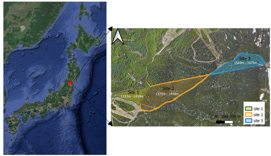
Figure 1.
The location of the study area in the Zao Mountains. Site 1 (mixed forest); Site 2 (transition from mix to monoculture forest); Site 3 (monoculture).
The mountain is covered by either pure conifer species Maries fir (Abies mariesii) which occupies about 87 percent of the forest area or is mixed with other coniferous and deciduous trees and shrubs (including Fagus crenata, Acer japonicum, Ilex crenata, Chengiopanax sciadophylloides, Taxus cuspidata, Pinus spp., Acer tschonoskii, Cornus controversa, Quercus crispula, and Sorbus commixta) (Table 1), while the lower vegetation layer is dominated by Sasa grass (dwarf bamboo) [24]. With increasing altitude, the vegetation composition along the mountain slope decreases in density and vegetation size.

Table 1.
Trees and shrubs species in Mt. Zao.
2.2. Data Acquisition and Pre-Processing
2.2.1. UAV Image Collection and Pre-Processing
The RGB images used in this study were taken during the autumn season (on 13 October 2022 and 12 October 2023), when the leaf color of the deciduous species changes. A DJI Mavic 2 Pro UAV equipped with a Hasselblad L1D-20c camera was used to collect the data. The UAV acquired 20-megapixel images, following routes designed on the application Drone Deploy (San Francisco, CA 94104, USA) at 90 m flying height using the terrain awareness function. The photos were acquired with 90% front and side overlaps. The camera was set at S priority (ISO-100) with shutter speed at 1/80–1/120 in case of favorable conditions and at 1/240–1/320 s in case of unfavorable conditions such as strong sun and wind. This setup kept exposure values (EV) of around 0 to +0.7, providing a ground sampling distance (GSD) of 1.5–2.1 cm/pixel. The total number of RAW images of Site 1, Site 2, and Site 3 flights were 287, 858 and 485 respectively. The raw RGB images collected from the forests were processed using Agisoft Metashape professional v1.7.4 (Agisoft LLC, Saint Petersburg, Russia) to create Orthomosaics (Figure 2), Dense Point Clouds and DEMs (Digital Elevation Models).
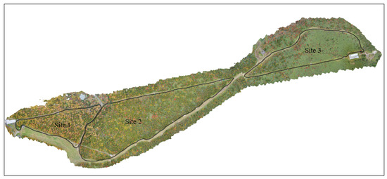
Figure 2.
The orthomosaics were generated using raw RGB photos in Metashape software v2.1.3.
Finally, the software Global Mapper v21.1, 64-bit (Blue Marble Geographic, Hallowell, ME, USA) was used to generate 3D Models (Three Dimensional Models) (Figure 3).
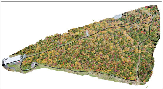
Figure 3.
The figure shows the 3D model of Site 1 was generated from the DPC.
The 3D model represents the study area in the view with gridded elevation data and any overlying raster or vector data in a true perspective 3D format. In particular, the sample plots can be selected and rotated to have a better look from directions (Figure 4).
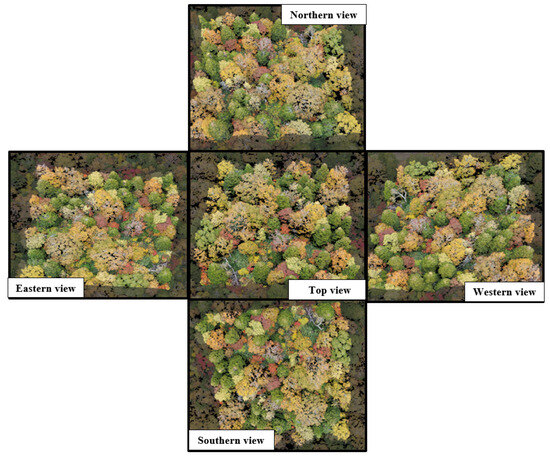
Figure 4.
The 3D Models of Plot 4 with 5 directions, facilitating vegetation visualization.
After the 3D Models were created, the last step was the creation of the CHMs, which represent the height of the trees and shrubs within each plot (Figure 5).
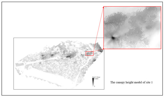
Figure 5.
The Canopy Height Models (CHMs) were generated using 3D Models with the software Global Mapper v21.1.
2.2.2. Field Data Collection
Map posters of plots within each site were printed in A4 and A0 sizes. We printed A0 size posters (extend 84.1 cm in width and 118.9 cm in height) of the orthomosaic for each site and A4 size (extend 21 cm in width and 29.7 cm in height) for each plot to validate the digital data with the ground truth field data (Figure 6).
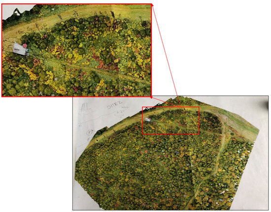
Figure 6.
An example for one of the posters that were used for fieldwork purposes.
Field Surveys
Fieldwork was conducted to validate the vegetation that had been identified in the orthomosaics. When accessibility limited the validation of vegetation in situ, a DJI mini 3 pro UAV was used to fly at a lower height (from 15 to 20 m) to take photos of a specific tree and shrub to validate the vegetation. Weighing only around 249 g, it featured robust obstacle avoidance capabilities. Additionally, it boasted a camera with a 1/1.3-inch CMOS sensor and an f/1.7 lens, enabling it to capture RAW images at 12 or 48 MP without any ghosting. These attributes made it an effective supporting instrument for our field surveys, particularly in the realm of plant identification. During these surveys, we validated vegetation by cross-referencing the manual annotation with the ground truth data to confirm the type of vegetation, the number of tree species, colors, and canopy shape.
2.2.3. Processing Data
Setting Plots and Individual Tree Detection
In this study, 14 plots, each of 50 m × 50 m, were randomly selected along the altitudinal gradient of the slope (Figure 7). Within these plots, individual tree species were meticulously identified and manually annotated. Due to the intricate structure of the forest, which included the overlapping of upper layers obscuring smaller trees in the understory layer, some smaller trees may have been overlooked.
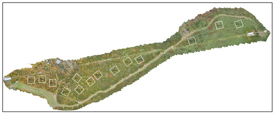
Figure 7.
Fourteen sample plots were set up in the study area regarding the increase in elevation.
Annotation, a crucial step in data preparation, was undertaken using RGB orthomosaic images (in .tif format) and 3D Models in QGIS (version 3.24.3, Tisler, 2022.02.18). A Shapefile layer was created for each species, denoted as “treecanopy.name of the plant”, to annotate all vegetation within the sample plots. Tree canopies were delineated by drawing polygons around individual trees. The technological workflow of the individual tree image annotation method is shown below (Figure 8).
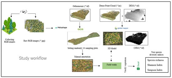
Figure 8.
Workflow in this study.
2.3. Diversity Measurement
Vegetation diversity represents the variety and abundance of distinct vegetation within a given ecosystem or area. It can be assessed across various spatial scales, including alpha diversity (within a specific habitat), beta diversity (between different habitats), and gamma diversity (multiple ecosystems or habitats at a regional or landscape level) [25]. There are various indices that can be used to measure species diversity, with some of them emphasizing a particular aspect of diversity. However, combining indices can provide a comprehensive point of view about species diversity in a given ecosystem or community. The diversity indices can be chosen depending on the specific purposes of the research and the type of data collected. In this study, the richness, abundance, and evenness of tree species within a specific habitat were evaluated by species richness (S), Simpson’s Diversity Index (D), and the Shannon–Wiener Diversity Index (H or H’).
2.3.1. Simpson’s Diversity Index (D)
Furthermore, Simpson’s Diversity Index (D) is considered both species richness and the abundance of each species, as it can be used as a measure of species dominance.
The formula for Simpson’s Diversity Index is typically expressed as:
where:
D represents the Simpson Index
represents the number of individuals of a particular species
N represents the total number of individuals in the community
Values of the index range from 0 to 1, and a higher D indicates greater diversity or evenness in a community, while a lower index implies less diversity and greater dominance by one or a few species (Figure 1 indicates the maximum diversity (all species are equally represented).
2.3.2. Shannon–Wiener Diversity Index (H or H’)
The other measure is the Shannon–Wiener Diversity Index (H or H’), which shows both species richness and evenness. It gives more weight to less abundant species, providing a measure of both the number of species and their relative abundances.
The Shannon index is calculated using the following formula:
where:
H represents the Shannon Diversity Index.
represents the proportion of individuals of species i relative to the total number of individuals in the community.
ln() represents the natural logarithm of .
In this case, values of the index range from 0 to 5, usually ranging from 1.5 to 3.5. A higher H value indicates more diversity, with more equally distributed species, while a lower H value implies lower diversity or the dominance of a few species.
2.3.3. Species Richness (S) Index
One of the simplest and straightforward measures of species diversity is the species richness (S) index. It represents the total number of different species present in a specific location.
Species Richness (S) = Number of different species
The first step is determining the number of species (S) and individuals of each species, which are the basic figures used to measure all indices.
2.3.4. Tree and Shrub Species
In total, the 12 tree and shrub species that are identified in the elevational gradient were annotated using QGIS. Thus, 12 shapefile layers were generated within the selected 50 m × 50 m plots. Tree and shrub species were meticulously annotated, classified, and counted manually. Subsequently, in the combination with Canopy Height Models (CHMs) data, the treetops were identified by utilizing the “Raster analysis” tool to determine the highest pixel value within each polygon in QGIS, thus obtaining the corresponding tree height measurements.
3. Results
3.1. Individual Tree and Shrub Detection
In this study, the main purposes of the vegetation identification process are tree and shrub annotation and corresponding height estimation. All tree and shrub species and the number of individuals of each one of them within the selected plots were recorded for the vegetation diversity analysis. Additionally, the forest structure was assessed using the CHM data (Table 2).

Table 2.
Summary of the number of trees and shrubs in each plot.
Species compositions were analyzed in detail for each plot (Figure 9). Within the altitude range (1344–1382 m.a.s.l) encompassing Plot 1 to Plot 3, eight types of vegetation were found, but their distribution was not uniform. This area was covered mainly by large Fagus crenata, and A. mariesii trees with the canopy coverage of approximately 50% of the total species composition in Plots 1 and 2, and nearly 70% in Plot 3. In contrast, vegetation such as Ilex crenata, C. sciadophylloides, and A. japonicum constituted a smaller percentage. In particular, Ilex crenata made up 1%, 6%, and 2% of the total species composition in Plot 1, Plot 2, and Plot 3, respectively. Similarly, Acer japonicum comprised 2–3% of the total in Plots 1, 2, and 3. At higher elevations (from Plot 4), shrub species became more prevalent, while Abies mariesii became the dominant tree species as Fagus crenata did not grow above this altitude. Notably, A. tschonoskii and Q. crispula emerge as dominant shrub species, constituting nearly half of the species composition in Plots 4 and 11. In Plot 7 and Plot 10, Q. crispula made up almost a third of all the individuals present in these plots. The number of A. tschonoskii shrubs is consistently prevalent in the elevation ranging from 1415 m to 1618 m (Plot 5 to Plot 12), making it one of the top three species with the highest number of individuals in these plots. However, as we reached the highest plots (Plot 13 and Plot 14), the number of A. tschonoskii individuals decreased while Q. crispula was not present anymore, thus yielding ground to Taxus cuspidata, which overwhelmingly dominated the majority of plots. In our study, we identify two Acer. species: Acer japonicum and Acer tschonoskii. Although Acer japonicum is not abundant, it is distributed from 1344 m (Plot 1) to 1483 m (Plot 11). In contrast, Acer tschonoskii is one of the dominant shrub species found from Plot 4 to Plot 14. Additionally, at the top of the mountain, particularly in Plot 13 (1592 m–1618 m) and Plot 14 (1637 m–1653 m), shrubs belonging to Salix species were found. Abies mariesii trees were the unique species found from Plot 1 to Plot 14. As the forest transitions from a mixed composition at lower elevations to a monoculture at higher elevations, the sensibility of the forest toward disturbances increases. This heightened sensitivity likely contributed to the high tree mortality rate caused by bark beetle infestation in the last decade.
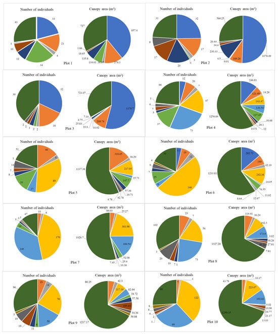
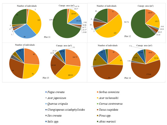
Figure 9.
The number of individuals and the canopy area of dominant species in the 14 plots along the altitudinal gradient.
Even though the number of Abies and F. crenata trees was small, their canopy area covered the majority of the area in a single plot (Figure 9). In contrast, shrubs species such as Quercus crispula and Acer tschonoskii exhibited a high number of individuals but covered smaller canopy areas.
The number of trees and shrubs peaked at Plot 7, reaching approximately 400 individuals in total, followed by Plot 10 and Plot 13 with 346 and 324 individuals, respectively. In addition, Plots 4 and 5 showed the highest species richness in the study area, with 11 species present. In contrast, Plots 12, 13, and 14 showed the lowest species diversity, with seven species identified, representing the change in the species richness and the number of individuals along the elevation gradients (Figure 10). There is a slight fluctuation in the number of species between the plots at lower and higher altitudes, but vegetation was different. For instance, although there were seven species present in Plots 12, 13, and 14, the vegetation identified in Plot 12 included Sorbus commixta, Acer tschonoskii, Chengiopanax sciadophylloides, Ilex crenata, and Abies mariesii. In contrast, Chengiopanax sciadophylloides was not observed in Plots 13 and 14; instead, Salix spp. was present in these plots.
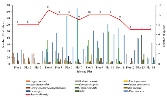
Figure 10.
Change in tree species composition at different altitude layers within the study area.
3.2. Tree Height and Elevation
A negative correlation was observed between tree height and elevation, as evidenced by the transition of some trees into shrub form at higher elevations (Table 3). The deviation in vegetation height for individual species indicates the differences from both the average height and the heights of individual plants within a selected plot (Table 4 and Table 5).

Table 3.
Average vegetation height in the 14 selected plots.

Table 4.
The average tree height and standard deviation from plot 1 to plot 7.

Table 5.
The average tree height and standard deviation from plot 8 to plot 14.
At lower elevations ( from 1337 m to 1407 m), Abies mariesii, Fagus crenata, Chengiopanax sciadophylloides, Sorbus commixta stood out as the four tallest tree species, with the average height of 12.2 m, 11.9 m, 9.9 m, 9.1 m respectively, while Acer japonicum, Cornus controversa, and Taxus cuspidata showed nearly identical average heights of approximately 7 m; Ilex crenata was the species occupying the lowest layer, with a height of around 6.1 m. In the elevation ranging from 1407 m to 1550 m, there is a decrease in the height of all species, with a change of approximately 4 m. At higher elevations (1550 m to 1654 m), species tend to be even smaller, with an average height ranging from 1 to 3 m. Vegetation such as Taxus cuspidata and others were considered shrubs.
Vegetation was identified and classified manually in QGIS and subsequently validated during fieldwork. The number of individuals for each vegetation type was counted from each shapefile layer. The results were used for assessing tree species diversity across the whole study area.
The diversity indices were computed by integrating data from individual tree and shrub species with computer vision identification, along with fieldwork validation for each plot. Although the calculated values indicate a minimal disparity between the low and high elevation plots, a slight decrease was observed at higher elevations (especially in Plots 12 to 14). Analysis of vegetation distribution across different plots revealed that those located between 1460 m and 1653 m (from Plot 10 to Plot 14) showed the lowest Shannon and Simpson diversity indices. Moreover, Plot 12 to Plot 14 (1524 m to 1653 m) had the lowest species richness value. In contrast, Plots 4 and 5 (spanning from 1407 m to 1426 m), as well as Plot 9 (ranging from 1439 m to 1457 m), demonstrated the highest values for alpha-diversity (Figure 11).
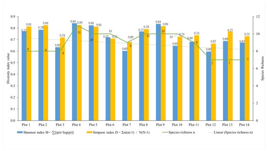
Figure 11.
Change in alpha-diversity indices in the plots along the altitudinal gradient (1336–1667 m).
3.2.1. Simpson Diversity Index
Based on the definition, the Simpson diversity index is a measure of diversity that takes into account the number of species present as well as the relative abundance of each species. Although the values of this index were higher than the Shannon index, they also varied with elevation. The same trend was observed in line with other indices. The most abundant areas were found at elevations ranging from 1407 m to 1426 m with the corresponding Simpson index value of 0.81 to 0.83. In these areas, the forests consisted of mixed vegetation with predominantly tall trees. The Simpson index value is lower in Plots 12 to 14 because of the high fir tree mortality rate caused by severe bark beetle infestation (elevation ranging from 1524 m to 1653 m).
3.2.2. Shannon Diversity Index
The Shannon diversity index considers both the abundance and evenness of species present in a given area. In this study, the Shannon index was used to assess the change in diversity along the altitude gradients, which have different environmental conditions. It displayed a decreasing trend with altitude, reaching the highest value in Plots 4 and 9 (0.84) and the lowest in Plots 7 and 12 (0.6), showing a high variability where altitude was not the only limiting factor for species abundance and evenness. Notably, although eight species were recorded in Plot 7, some species had very few individuals, resulting in low species diversity as measured by the Shannon index. In contrast, Plots 4 and 9 had both the highest species richness (11 and 10 species respectively) and the highest Shannon index value due to the evenness in the number of individual tree species. The Shannon diversity index indicated that Plot 13 had the most abundant and equally distributed vegetation composition (0.69). However, overall, the Shannon diversity index exhibited a decreasing trend with increasing elevation.
3.2.3. Species Richness
The alpha diversity, species richness is one of the most important indices that expresses the number of species in a given plot. The species richness in Plots 1 to 3 (with eight species each) was lower than those of Plots 4 to 10 (ranging from 9 to 11 species of the total 12 identified). On the other hand, the number of vegetation types decreased to 7 at Plots 12, 13, and 14.
4. Discussion
4.1. Vegetation Distribution
The diversity of tree species plays an essential role in maintaining the health and resilience of forest ecosystems to natural disturbances. In this study, we successfully estimated tree species diversity and construct the 3D structure of the forest in Zao Mt. using UAV-acquired RGB imagery. Ref. [26] found a strong correlation between tree size and tree species diversity in subtropical forests, indicating a positive and independent relationship with habitat. They computed alpha diversity indices and observed a clear relationship with tree diameter at breast height (DBH). However, in our study, we could not find a negative or positive correlation between vegetation height (we used vegetation height as a proxy for vegetation size) and species diversity.
Elevation thresholds were observed for most of the vegetation in the study area, highlighting the significant impact of environmental conditions (temperature, soil properties, variability, precipitation, and solar radiation) [27,28], elevation, and slope on the ecological characteristics of specific areas. As altitude increases, temperature (approximately 0.65 °C per 100 m of elevation) as well as air pressure tend to decline [29], while precipitation often rises, leading to different distribution patterns of vegetation across elevation gradients. Evidence indicates that elevation significantly influences vegetation distribution, which may relate to variations in many environmental factors and plant species adaptation characteristics [30,31]. In our study, one of the most obvious tree species was Fagus crenata because of its size; and it could be found occupying large areas from 1334 m to 1426 m but be completely absent at higher elevations. This observation is relevant for understanding vegetation expansion as a result of climate change, particularly in higher altitudes where warming trends are more pronounced [32,33,34,35]. The increasing temperatures contribute to accelerated snowmelt and reduced snow accumulation, which together may promote vegetation growth and facilitate the upward expansion of ecological thresholds. In the hypothetical case that air temperature continues increasing the threshold line defined for some tree or shrub species in this study might shift to higher elevations [36,37,38,39,40] or grow larger in the future. The same can be observed for other vegetation such as Quercus crispula, which, unlike Fagus crenata, was always found in a shrub form and distributed from 1407 m to 1483 m. In addition, species such as Cornus controversa and Acer jacponicum are abundant at the elevation range of 1334 m to 1483 m, but they cease to grow at higher elevations. Both species are not suited for high altitude environmental conditions. In contrast, Salix spp. was found only at higher elevations (ranging from 1592 m to 1653 m). In this study, Abies mariesii is the species distributed in the whole study area (from 1334m to 1653 m), although the number of individual trees decreased and became scattered at higher elevations. The only two species that were found in all the plots besides Abies mariesii were Sorbus commixtra and Ilex cranata. In the study area, Abies mariesii individuals found at elevations above 1550 m were predominantly saplings. Although mature dead trees are still standing, they no longer contribute to forest biodiversity. Highlighting the importance of insect outbreaks as an agent of change in vegetation dynamics. Bark beetle infestation caused a high mortality rate in Plots 12 to 14 and has slowly but steadily moved downwards as it is also observed by dead trees found in Plots 4 to 11; there is a relatively low mortality in Plots 1 to 3. The high mortality inflicted on Abies mariesii has impacted species diversity in the plots where, first, Abies mariesii trees are not present anymore and, second, the expansion in the proportion of the area is covered by the remaining shrub vegetation in the respective plots. Positioned at the highest elevation, Site 3 represents the most vulnerable area as it was severely damaged by bark beetle infestation from 2012 to 2016 [24]. In Plots 12 to 14, the average vegetation height was less than 4 m and at present—the vegetation is predominantly composed of shrub species, where the indices for species diversity exhibited a declining trend compared to the lower elevation plots.
4.2. Alpha Diversity Indices
The results of this study indicated that changes in tree and shrub size, with increasing elevation, were influenced by environmental conditions, which in turn affect species diversity. In the mixed forest at lower altitudes, deciduous trees are dominant, creating a competitive environment that challenges the growth of evergreen species, which typically exist as shrubs. These shrub species struggle to adapt to the shaded conditions, which explains the absence of certain species in these areas, such as Fagus crenata, Acer japonicum, and Quercus crispula [41,42] implied that the decrease in species richness and diversity was linked to increases in elevation. However, recent studies indicate that vegetation diversity indices often vary and reach their highest value at mid-elevations [30,31,43,44]. In our study, the diversity indices similarly exhibited a weak correlation with altitude, corresponding with the above findings. At lower elevations (Plot 1 to Plot 3), the Shannon index, the Simpson index and the species richness were in average 0.73, 0.78 and 8 respectively, while at higher elevations (Plot 12 to Plot 14) the same indices were 0.65, 0.72 and 7. In between these altitude ranges, the same indices were 0.74, 0.76, and 10, respectively. As it can be observed the Shannon index and Simpson index at higher elevations were just slightly lower than at lower elevations, especially the Shannon index which represents the evenness of species showed its lowest value in Plot 12, however, similar values were found in Plot 7 and 10 (0.6 and 0.65, respectively). The species richness is one of the indices that represents the number of different species. In our study, the value was the same at low as well as at high elevations; however, the vegetation types, except for Abies mariesii and Sobus commixta, were different. These findings also indicated the impacts of environmental conditions on the species diversity. Air temperature along the altitudinal gradient is the most important parameter that controls vegetation distribution in the Zao Mountains. Vegetation that is able to thrive under a warmer regime was found in lower altitudes and included Fagus crenata, Quercus crispula, and Cornus controversa, while more low temperature vegetation, such as Salix spp., were found at high altitudes. Those able to thrive along the whole altitudinal range, such as Acer tschonoskii and Sorbus commixta, showed wide thermal tolerance, although at higher altitudes, vegetation size decreases. As the results showed both lower and higher altitudes where the temperature was extreme, the vegetation diversity indices were limited [45] (especially species richness). While in the mid-elevation, where the temperatures were milder and suitable for more species, a more diverse ecosystem was created [46]. Even though precipitation was not measured along the altitude gradient, there appears to be negligible difference among the plots. However, lower snow depth and especially earlier snow melting in steep slopes, which are exposed to strong western winds and solar radiation, might limit soil water availability in the usually dry spring months of Zao Mountains. That could be an additional limiting factor for some of the vegetation, especially in Site 3 (Plots 12–14). It is worth mentioning that these characteristics might have been responsible for the fir forest vulnerability to the bark beetle attack reported for this same site for the period 2012–2016 [24,47]. The Zao Mountains in Japan are unique because they are the only area in Japan where bark beetle infestation has caused a high mortality rate in the treeline, and it is representative of the Ōu Mountain Range that divides northeastern Japan between east and west. Since there has been no study analyzing vegetation distribution based on altitude or latitude gradients in this area, this study constitutes the first large-scale and detailed study on vegetation distribution and can become the basis for comparative studies with other similar regions in northeastern Japan first and then with other regions in Japan.
In this study, we considered not only the number of different species but also the individuals present in a given plot that represent the abundance and evenness of the vegetation within the study area. Although the Shannon index and Simpson index both consider species abundance, what they assess is different. The Shannon index tends to be more sensitive to rare species, while the Simpson index is more influenced by the most common species. In the majority of the analyzed plots, Shannon index values were observed to be lower than Simpson index values. This discrepancy indicates an uneven distribution of species within these plots, where some species are significantly more abundant than others. It is notable that Plots 13 and 14 demonstrated relatively low Shannon index values (0.69 and 0.67, respectively) compared to their Simpson index values (0.77 and 0.73, respectively). Despite the high total number of individuals (354 in Plot 13), the distribution was highly uneven. For instance, Plot 13 contained 155 individuals of Acer tschonoskii and only one sapling of Abies mariesii. Although Abies mariesii is the dominant species in the forest, its presence in both Plots 13 and 14 has been severely impacted by bark beetle infestations during the last decade, thus influencing the overall species composition and distribution within these plots. Although dead Abies mariesii trees may persist as standing snags, they do not contribute to the current species diversity of the forest. In contrast, the presence of Abies mariesii saplings can indicate the process of forest regeneration following the bark beetle infestation. Despite their low abundance, these saplings serve as a sign of the species’ recovery and its potential role in reestablishing ecological functions within the forest. In contrast, Plots 4, 5, 6, and 9 (ranging from 1407 m to 1426 m and 1439 m to 1457 m) exhibited higher Shannon index values relative to Simpson index values, suggesting greater species diversity and more balanced distribution among species. Specifically, Plots 4, 5, and 9 had high total numbers of individuals (281, 269, and 311, respectively) and also displayed relatively high evenness among species.
Overall, vegetation in the plots showed high variability: some plots exhibited high species richness and evenness, and others may have high species richness but with uneven distribution, leading to differences in diversity indices. In this context, the interplay between species richness and evenness is crucial for accurately assessing and interpreting biodiversity in these areas. This pattern suggests that in most of the forest plots, the evenness of species distribution was relatively low. This variability may be attributed to micro environment, micro climate, and micro relief that also influenced vegetation distribution.
4.3. Challenges during the Field Surveys
Zao Mountains are characterized by rugged terrain and steep slopes, which present unique challenges for biodiversity assessment. The complex topography, coupled with the dense vegetation and diverse species composition, complicates efforts to accurately assess the region’s biodiversity. One of the primary challenges in biodiversity assessment on Zao Mountain is the difficulty in accessing and validating species data. The dense understory vegetation, composed of a mix of canopy shapes and sizes, presents challenges in species identification. This heterogeneity often results in overlooked individuals, leading to gaps in the identified data. The presence of Sasa grass, with an average height of 2 m and covering the forest floor, further complicates biodiversity assessment. When conducting this study, we found that RGB imagery, while valuable for capturing tree-top views, has limitations when it comes to canopy penetration. In dense forest areas, the tangled complexity of tree branches and the height of the Sasa grass obstruct the view, making it difficult to identify species from above. As a result, ground points became the primary data source for biodiversity assessment, highlighting the need for complementary data collection methods such as LiDAR or UAV-based remote sensing, which includes multispectral or hyperspectral imagery. Multispectral and hyperspectral data, with their varying wavelength bands, provide both geometric and spectral information about vegetation. When combined with LiDAR data, which excels in topography and 3D surface features, this integration improves vegetation detection and classification, resulting in higher reliability and accuracy [48,49,50,51]. Another significant challenge faced during fieldwork is the unpredictability of encountering dangerous wildlife. In addition, although summer and autumn are the best periods for the validation procedure, the weather is highly variable, with rain, fog, and strong winds making data collection and vegetation validation difficult. All these highlight the complexities of studying natural forest ecosystems, but with the use of UAV technology, it is possible to understand and map vegetation distribution of large areas with relatively high precision. The next step for reducing the fieldwork hurdles and limitations will be the development of Deep Learning Models that can facilitate automatic surveys of large areas.
5. Conclusions
In this study, we successfully used the capacity of UAV high-resolution RGB imagery to identify individual species and assess alpha-diversity indices in the large-scale area in the Zao Mountains. The results of this study showed the potential of RGB imagery to classify vegetation and calculate tree species diversity with high accuracy, which can provide essential information for understanding biodiversity and achieving sustainable forest management. This is the first study of its kind in the Zao Mountains, and its results can be used to better understand vegetation distribution in the mountainous areas of Japan.
Several findings were confirmed that are consistent with previous studies. First, tree and shrub size reduction, with increasing altitude, affected species diversity indices, especially the Shannon index, which is related to the evenness of vegetation. Second, the distribution of the different ranges of representative subalpine trees and shrub species of mountains in Japan was clearly determined based on their altitude range.
Third, a weak negative relationship was observed between tree species diversity and elevation. Specifically, species diversity indices increased with altitude at lower elevations, peaked at mid-elevation, and then declined at higher elevations. Both species richness and the Simpson and Shannon diversity indices were significantly higher at mid-elevation, reflecting a suitable environment for more species to exist.
Future research could investigate the combination of UAV RGB imagery with other data sources, such as LiDAR, multispectral, or hyperspectral data, to determine if they can be applied to a broader range of ecosystem monitoring and enhance the accuracy and reliability of the species diversity calculation. Additionally, exploring the integration of these data sources with technologies such as machine learning or deep learning for automated vegetation classification could further enhance the efficiency and accuracy of detection.
Author Contributions
Conceptualization: [T.C.N.T.], Methodology: [T.C.N.T., M.L.L.C.], Software: [S.G.i.R., M.C., Y.D.], Validation: [T.C.N.T., M.L.L.C.], Formal Analysis: [T.C.N.T.], Resources: [S.G.i.R., T.C.N.T., M.L.L.C.], Data Curation: [T.C.N.T.], Writing—Original Draft: [T.C.N.T.], Writing—Review and Editing: [M.L.L.C., T.C.N.T.], Supervision: [M.L.L.C., Y.K., C.-Y.T.]. All authors have read and agreed to the published version of the manuscript.
Funding
This research received no external funding.
Data Availability Statement
Data sharing is not applicable to this article.
Acknowledgments
We gratefully acknowledge the support provided by the members of the Smart Forest Laboratory for data collection, vegetation validation during fieldwork surveys, and software processes. Their contributions were crucial to the success of this research. We also extend our thanks to the anonymous reviewers for their insightful comments and suggestions, which greatly enhanced the quality of this manuscript.
Conflicts of Interest
The authors declare no conflicts of interest.
Correction Statement
This article has been republished with a minor correction to the authorship. This change does not affect the scientific content of the article.
Abbreviations
| CHM | Canopy Height Model |
| DBH | Diameter at breast height |
| DEM | Digital Elevation Model |
| RGB | Red Green Blue |
| UAV | Unmanned Aerial Vehicle |
References
- Chirici, G.; McRoberts, R.E.; Winter, S.; Bertini, R.; Brändli, U.B.; Asensio, I.A.; Bastrup-Birk, A.; Rondeux, J.; Barsoum, N.; Marchetti, M. National forest inventory contributions to forest biodiversity monitoring. For. Sci. 2012, 58, 257–268. [Google Scholar] [CrossRef]
- Gyamfi-Ampadu, E.; Gebreslasie, M.; Mendoza-Ponce, A. Evaluating multi-sensors spectral and spatial resolutions for tree species diversity prediction. Remote Sens. 2021, 13, 1033. [Google Scholar] [CrossRef]
- Arekhi, M.; Yılmaz, O.Y.; Yılmaz, H.; Akyüz, Y.F. Can tree species diversity be assessed with Landsat data in a temperate forest? Environ. Monit. Assess. 2017, 189, 586. [Google Scholar] [CrossRef]
- Jactel, H.; Bauhus, J.; Boberg, J.; Bonal, D.; Castagneyrol, B.; Gardiner, B.; Gonzalez-Olabarria, J.R.; Koricheva, J.; Meurisse, N.; Brockerhoff, E.G. Tree diversity drives forest stand resistance to natural disturbances. Curr. For. Rep. 2017, 3, 223–243. [Google Scholar] [CrossRef]
- Trogisch, S.; Liu, X.; Rutten, G.; Xue, K.; Bauhus, J.; Brose, U.; Bu, W.; Cesarz, S.; Chesters, D.; Connolly, J.; et al. The significance of tree-tree interactions for forest ecosystem functioning. Basic Appl. Ecol. 2021, 55, 33–52. [Google Scholar] [CrossRef]
- Bauhus, J.; Forrester, D.I.; Gardiner, B.; Jactel, H.; Vallejo, R.; Pretzsch, H. Ecological stability of mixed-species forests. In Mixed-Species Forests: Ecology and Management; Springer: Berlin/Heidelberg, Germany, 2017; pp. 337–382. [Google Scholar]
- Ouyang, S.; Xiang, W.; Gou, M.; Chen, L.; Lei, P.; Xiao, W.; Deng, X.; Zeng, L.; Li, J.; Zhang, T.; et al. Stability in subtropical forests: The role of tree species diversity, stand structure, environmental and socio-economic conditions. Glob. Ecol. Biogeogr. 2021, 30, 500–513. [Google Scholar] [CrossRef]
- Yang, L.; Zhang, J.; Wang, J.; Gu, Y.; Han, S. A linear positive relationship between tree species diversity and forest productivity across forest-dominated natural reserves on a large spatial scale. For. Ecol. Manag. 2023, 548, 121409. [Google Scholar] [CrossRef]
- Tariku, G.; Ghiglieno, I.; Gilioli, G.; Gentilin, F.; Armiraglio, S.; Serina, I. Automated identification and classification of plant species in heterogeneous plant areas using unmanned aerial vehicle-collected RGB images and transfer learning. Drones 2023, 7, 599. [Google Scholar] [CrossRef]
- Buhk, C.; Retzer, V.; Beierkuhnlein, C.; Jentsch, A. Predicting plant species richness and vegetation patterns in cultural landscapes using disturbance parameters. Agric. Ecosyst. Environ. 2007, 122, 446–452. [Google Scholar] [CrossRef]
- Chai, M.M.F.; Bayat, S.; Hashemi, S.A. Probability measurement to estimate forest tree diversity using IRS-p6 satellite images in Caspian broad leaved forests. J. Agric. Biol. Sci. 2012, 7, 238–243. [Google Scholar]
- Dalmayne, J.; Möckel, T.; Prentice, H.C.; Schmid, B.C.; Hall, K. Assessment of fine-scale plant species beta diversity using WorldView-2 satellite spectral dissimilarity. Ecol. Inform. 2013, 18, 1–9. [Google Scholar] [CrossRef]
- Liu, K.; Wang, A.; Zhang, S.; Zhu, Z.; Bi, Y.; Wang, Y.; Du, X. Tree species diversity mapping using UAS-based digital aerial photogrammetry point clouds and multispectral imageries in a subtropical forest invaded by moso bamboo (Phyllostachys edulis). Int. J. Appl. Earth Obs. Geoinf. 2021, 104, 102587. [Google Scholar] [CrossRef]
- Saarinen, N.; Vastaranta, M.; Näsi, R.; Rosnell, T.; Hakala, T.; Honkavaara, E.; Wulder, M.A.; Luoma, V.; Tommaselli, A.M.; Imai, N.N.; et al. Assessing biodiversity in boreal forests with UAV-based photogrammetric point clouds and hyperspectral imaging. Remote Sens. 2018, 10, 338. [Google Scholar] [CrossRef]
- Gimaret-Carpentier, C.; Pélissier, R.; Pascal, J.P.; Houllier, F. Sampling strategies for the assessment of tree species diversity. J. Veg. Sci. 1998, 9, 161–172. [Google Scholar] [CrossRef]
- Kanagaraj, S.; Selvaraj, M.; Das Kangabam, R.; Munisamy, G. Assessment of tree species diversity and its distribution pattern in Pachamalai Reserve Forest, Tamil Nadu. J. Sustain. For. 2017, 36, 32–46. [Google Scholar] [CrossRef]
- Motz, K.; Sterba, H.; Pommerening, A. Sampling measures of tree diversity. For. Ecol. Manag. 2010, 260, 1985–1996. [Google Scholar] [CrossRef]
- Baraloto, C.; Molto, Q.; Rabaud, S.; Hérault, B.; Valencia, R.; Blanc, L.; Fine, P.V.; Thompson, J. Rapid simultaneous estimation of aboveground biomass and tree diversity across Neotropical forests: A comparison of field inventory methods. Biotropica 2013, 45, 288–298. [Google Scholar] [CrossRef]
- Li, X.; Zheng, Z.; Xu, C.; Zhao, P.; Chen, J.; Wu, J.; Zhao, X.; Mu, X.; Zhao, D.; Zeng, Y. Individual tree-based forest species diversity estimation by classification and clustering methods using UAV data. Front. Ecol. Evol. 2023, 11, 1139458. [Google Scholar] [CrossRef]
- Michałowska, M.; Rapiński, J. A review of tree species classification based on airborne LiDAR data and applied classifiers. Remote Sens. 2021, 13, 353. [Google Scholar] [CrossRef]
- Lu, T.; Brandt, M.; Tong, X.; Hiernaux, P.; Leroux, L.; Ndao, B.; Fensholt, R. Mapping the abundance of multipurpose agroforestry Faidherbia albida trees in Senegal. Remote Sens. 2022, 14, 662. [Google Scholar] [CrossRef]
- Shang, X.; Chisholm, L.A. Classification of Australian native forest species using hyperspectral remote sensing and machine-learning classification algorithms. IEEE J. Sel. Top. Appl. Earth Obs. Remote Sens. 2013, 7, 2481–2489. [Google Scholar] [CrossRef]
- Treuhaft, R.N.; Asner, G.P.; Law, B.E.; Van Tuyl, S. Forest leaf area density profiles from the quantitative fusion of radar and hyperspectral data. J. Geophys. Res. Atmos. 2002, 107, ACL-7. [Google Scholar] [CrossRef]
- Nguyen, H.T.; Lopez Caceres, M.L.; Moritake, K.; Kentsch, S.; Shu, H.; Diez, Y. Individual sick fir tree (Abies mariesii) identification in insect infested forests by means of UAV images and deep learning. Remote Sens. 2021, 13, 260. [Google Scholar] [CrossRef]
- Whittaker, R.H. Communities and Ecosystems; Macmillan Company: London, UK; Collier-Macmillan Limited: London, UK, 1970. [Google Scholar]
- Li, Y.; Ye, S.; Luo, Y.; Yu, S.; Zhang, G. Relationship between species diversity and tree size in natural forests around the Tropic of Cancer. J. For. Res. 2023, 34, 1735–1745. [Google Scholar] [CrossRef]
- Körner, C. The cold range limit of trees. Trends Ecol. Evol. 2021, 36, 979–989. [Google Scholar] [CrossRef]
- Groffman, P.M.; Baron, J.S.; Blett, T.; Gold, A.J.; Goodman, I.; Gunderson, L.H.; Levinson, B.M.; Palmer, M.A.; Paerl, H.W.; Peterson, G.D.; et al. Ecological thresholds: The key to successful environmental management or an important concept with no practical application? Ecosystems 2006, 9, 1–13. [Google Scholar] [CrossRef]
- Barry, R.G. Mountain Weather and Climate; Cambridge University Press: Cambridge, UK, 2008. [Google Scholar]
- Gong, H.; Yu, T.; Zhang, X.; Zhang, P.; Han, J.; Gao, J. Effects of boundary constraints and climatic factors on plant diversity along an altitudinal gradient. Glob. Ecol. Conserv. 2019, 19, e00671. [Google Scholar] [CrossRef]
- LI, W.H.; Ganjurjav, H.; Cao, X.-J.; Yan, Y.; Li, Y.; Luo, W.-R.; Hu, G.; Danjiu, L.; He, S.-C.; Gao, Q. Effects of altitude on plant productivity and species diversity in alpine meadows of northern Tibet. Acta Prataculturae Sin. 2017, 26, 200. [Google Scholar]
- Tai, X.; Epstein, H.E.; Li, B. Elevation and climate effects on vegetation greenness in an arid mountain-basin system of Central Asia. Remote Sens. 2020, 12, 1665. [Google Scholar] [CrossRef]
- Liu, X.; Cheng, Z.; Yan, L.; Yin, Z.Y. Elevation dependency of recent and future minimum surface air temperature trends in the Tibetan Plateau and its surroundings. Glob. Planet. Chang. 2009, 68, 164–174. [Google Scholar] [CrossRef]
- Clow, D.W. Changes in the timing of snowmelt and streamflow in Colorado: A response to recent warming. J. Clim. 2010, 23, 2293–2306. [Google Scholar] [CrossRef]
- Ceppi, P.; Scherrer, S.C.; Fischer, A.M.; Appenzeller, C. Revisiting Swiss temperature trends 1959–2008. Int. J. Climatol. 2012, 32, 203–213. [Google Scholar] [CrossRef]
- Dullinger, S.; Dirnböck, T.; Grabherr, G. Modelling climate change-driven treeline shifts: Relative effects of temperature increase, dispersal and invasibility. J. Ecol. 2004, 92, 241–252. [Google Scholar] [CrossRef]
- Ryan, K.C. Vegetation and wildland fire: Implications of global climate change. Environ. Int. 1991, 17, 169–178. [Google Scholar] [CrossRef]
- Parolo, G.; Rossi, G. Upward migration of vascular plants following a climate warming trend in the Alps. Basic Appl. Ecol. 2008, 9, 100–107. [Google Scholar] [CrossRef]
- Felde, V.A.; Kapfer, J.; Grytnes, J.A. Upward shift in elevational plant species ranges in Sikkilsdalen, central Norway. Ecography 2012, 35, 922–932. [Google Scholar] [CrossRef]
- Walther, G.R.; Beißner, S.; Burga, C.A. Trends in the upward shift of alpine plants. J. Veg. Sci. 2005, 16, 541–548. [Google Scholar] [CrossRef]
- Song, X.; Cao, M.; Li, J.; Kitching, R.L.; Nakamura, A.; Laidlaw, M.J.; Tang, Y.; Sun, Z.; Zhang, W.; Yang, J. Different environmental factors drive tree species diversity along elevation gradients in three climatic zones in Yunnan, southern China. Plant Divers. 2021, 43, 433–443. [Google Scholar] [CrossRef]
- McCain, C.M.; Grytnes, J.A. Elevational gradients in species richness. In Encyclopedia of Life Sciences (eLS); John Wiley & Sons, Ltd.: Chichester, UK, 2010. [Google Scholar] [CrossRef]
- Zhou, Y.; Chen, S.; Hu, G.; Mwachala, G.; Yan, X.; Wang, Q. Species richness and phylogenetic diversity of seed plants across vegetation zones of Mount Kenya, East Africa. Ecol. Evol. 2018, 8, 8930–8939. [Google Scholar] [CrossRef]
- Rawat, B.; Gaira, K.S.; Gairola, S.; Tewari, L.M.; Rawal, R.S. Spatial prediction of plant species richness and density in high-altitude forests of Indian west Himalaya. Trees For. People 2021, 6, 100132. [Google Scholar] [CrossRef]
- Kluge, J.; Kessler, M.; Dunn, R.R. What drives elevational patterns of diversity? A test of geometric constraints, climate and species pool effects for pteridophytes on an elevational gradient in Costa Rica. Glob. Ecol. Biogeogr. 2006, 15, 358–371. [Google Scholar] [CrossRef]
- Gao, J.; Liu, Y. Climate stability is more important than water–energy variables in shaping the elevational variation in species richness. Ecol. Evol. 2018, 8, 6872–6879. [Google Scholar] [CrossRef]
- Moritake, K.; Cabezas, M.; Nhung, T.T.C.; Caceres, M.L.L.; Diez, Y. Sub-alpine shrub classification using UAV images: Performance of human observers vs DL classifiers. Ecol. Inform. 2024, 80, 102462. [Google Scholar] [CrossRef]
- Bork, E.W.; Su, J.G. Integrating LIDAR data and multispectral imagery for enhanced classification of rangeland vegetation: A meta analysis. Remote Sens. Environ. 2007, 111, 11–24. [Google Scholar] [CrossRef]
- Kukkonen, M.; Maltamo, M.; Korhonen, L.; Packalen, P. Multispectral airborne LiDAR data in the prediction of boreal tree species composition. IEEE Trans. Geosci. Remote Sens. 2019, 57, 3462–3471. [Google Scholar] [CrossRef]
- Budei, B.C.; St-Onge, B.; Hopkinson, C.; Audet, F.A. Identifying the genus or species of individual trees using a three-wavelength airborne lidar system. Remote Sens. Environ. 2018, 204, 632–647. [Google Scholar] [CrossRef]
- Shi, Y.; Skidmore, A.K.; Wang, T.; Holzwarth, S.; Heiden, U.; Pinnel, N.; Zhu, X.; Heurich, M. Tree species classification using plant functional traits from LiDAR and hyperspectral data. Int. J. Appl. Earth Obs. Geoinf. 2018, 73, 207–219. [Google Scholar] [CrossRef]
Disclaimer/Publisher’s Note: The statements, opinions and data contained in all publications are solely those of the individual author(s) and contributor(s) and not of MDPI and/or the editor(s). MDPI and/or the editor(s) disclaim responsibility for any injury to people or property resulting from any ideas, methods, instructions or products referred to in the content. |
© 2024 by the authors. Licensee MDPI, Basel, Switzerland. This article is an open access article distributed under the terms and conditions of the Creative Commons Attribution (CC BY) license (https://creativecommons.org/licenses/by/4.0/).