Abstract
Radar emitter signal deinterleaving based on pulse description words (PDWs) is a challenging task in the field of electronic warfare because of the parameter sparsity and uncertainty of PDWs. In this paper, a modulation-hypothesis-augmented Transformer model is proposed to identify emitters from a single PDW with an end-to-end manner. Firstly, the pulse features are enriched by the modulation hypothesis mechanism to generate I/Q complex signals from PDWs. Secondly, a multiple-parameter embedding method is proposed to expand the signal discriminative features and to enhance the identification capability of emitters. Moreover, a novel Transformer deep learning model, named PulseFormer and composed of spectral convolution, multi-layer perceptron, and self-attention based basic blocks, is proposed for discriminative feature extraction, emitter identification, and signal deinterleaving. Experimental results on synthesized PDW dataset show that the proposed method performs better on emitter signal deinterleaving in complex environments without relying on the pulse repetition interval (PRI). Compared with other deep learning methods, the PulseFormer performs better in noisy environments.
1. Introduction
Signal deinterleaving is the process of classifying and identifying multiple overlapping signals in complex electromagnetic environments based on specific criteria. The primary goal is to distinguish signals from different sources for further processing and analysis. In modern electronic warfare systems, identifying radar emitters by signal deinterleaving is particularly critical. However, in such complex electromagnetic environments, quickly and accurately classifying interleaved radar pulses remains a significant challenge in the field of electronic warfare [1]. Data received by electronic reconnaissance often contain a mixture of pulse descriptions, which is extracted from raw in-phase/quadrature (I/Q) signals and may include carrier frequency (CF), pulse width (PW), pulse amplitude (PA), direction of arrival (DOA), and time of arrival (TOA) [2,3]. The PDW is a concise representation of radar emitter signals. Meanwhile, these pulse description words (PDWs) provide critical information that helps to identify and distinguish different emitters to achieve effective jamming and counter-measuring in modern electronic warfare.
In recent years, deep learning has emerged as a powerful tool for signal processing tasks, including signal deinterleaving. Specifically, neural networks can be trained to learn to discriminate the emitters from the incoming interleaved pulses [4]. By analyzing the radio frequency fingerprinting of radar emitters, effective deinterleaving of different radar signals within the pulse trains can be achievable. Traditional methods often rely on manual feature extraction and rule-based algorithms, and most of them heavily rely on an inter-pulse parameter analysis (i.e., PRI, TOA etc.) based on the pulse trains, which can be time-consuming and less adaptable to complex and dynamic environments [5,6,7]. Deep learning models, particularly neural networks, can automatically learn and extract discriminative features from raw radar signals, significantly improving the efficiency and accuracy of emitter identification. However, directly inputting the concise form of PDWs into a deep neural model would result in model underfitting and could not effectively build enough discriminative space to identify each specific emitters.
Moreover, previous studies on radar signal deinterleaving based on intra-pulse modulation [8,9,10] inspired us to explore how to utilize the intra-pulse modulation to enhance the performance of signal deinterleaving. Among these methods, the paper [8] introduced a time-domain technique based on autocorrelation to identify exotic modulated signals by measuring instantaneous frequency and amplitude in real time. Then, these modulation types could be used as discriminative parameters for signal deinterleaving, significantly improving emitter identification accuracy in complex environments. Additionally, the studies presented in [9,10] also employed intra-pulse modulation types to identify emitters and achieved satisfactory results. Therefore, generating raw I/Q signals based on the hypothesized modulation parameters from PDWs is a natural idea to explore the novel signal deinterleaving method.
In this paper, we propose a novel data augmentation method to generate rich raw signals based on an hypothesis on the modulation types of emitters. Based on the generated I/Q signals, a PulseFormer deep learning model originated from the Transformer architecture [11,12] is trained on the PDW dataset and further used to classify the radar emitters. Specifically, the main contributions of this paper are summarized as follows:
- A data augmentation mechanism based on a modulation hypothesis of intra-pulse parameters is proposed to generate rich I/Q signals from a single PDW.
- An embedding method based on multiply parameters is proposed to enrich the emitter information to achieve more reliable signal deinterleaving.
- A spectral convolution-enhanced Transformer model based on local, global, and a noise-resisted feature representation learning mechanism is built for signal classification.
- Experimental results show that our method achieves state-of-the-art performance compared with previous methods without relying on PRI parameters.
The rest of this paper is organized as follows. Section 2 introduces related work on radar emitter signal deinterleaving. The problem of radar emitter signal deinterleaving is introduced in Section 3. In Section 4, the data augmentation strategy and a spectral convolution-enhanced Transformer model for signal deinterleaving are introduced. Data simulations and an experimental analysis are described in Section 5. Section 6 discusses the comparison of our method with previous methods and the broad impact in different scenarios. Finally, Section 7 concludes this work.
2. Related Work
Research on radar emitter signal deinterleaving can be divided into two categories of methods, one is based on TOA information and another is based on the multi-parameters of the inner pulse. This paper studies the deinterleaving method based on the multi-parameters of the inner pulse.
2.1. TOA-Based Deinterleaving Methods
The pulse repetition interval (PRI) of a radar is the time difference between the leading edges of successive pulses when the radar transmits a signal. In deinterleaving methods based on time of arrival (TOA), a crucial concept is leveraging the periodic nature of the radar PRI. This approach involves identifying the radar PRI or its periodicity from the difference in TOA (DTOA) of the pulse sequence and then using the identified PRI or periodicity to extract the target radar pulses from the pulse sequence [1,4,5,6,7,13,14,15,16,17,18,19,20,21,22].
Among signal deinterleaving methods based on TOA parameters, typical traditional methods, such as PRI histograms [5,6] and PRI transformations [7], can yield preliminary results. However, these methods often require extensive expert knowledge for parameter tuning, making them less suitable for more general and complex scenarios. Subsequently, radar pulse streams characterized by periodic PRIs have been typically modeled using linear dynamic systems, with deinterleaving performed through the use of Kalman filters [13,14]. Furthermore, some studies [15,16] have employed hidden Markov models (HMMs) to address radar signal deinterleaving. Despite their effectiveness, these approaches heavily rely on specific assumptions being met, and their complexity can hinder practical implementation. Clustering techniques have also been applied to signal deinterleaving. For instance, in [17], a radar emitter recognition method based on clustering methods combined with decision tree classification was proposed. However, this method depended on pre-configured parameters such as manual thresholds and splitting criteria, which may require further manual tuning in real-world applications.
In recent years, deep learning [1,4,18,19,20,21,22] methods have been extensively applied to the task of radar signal deinterleaving. Among them, refs. [1,18,19] employed Recurrent Neural Networks (RNNs) to extract high-level features from pulse sequences, enabling effective identification between emitters based on sequence characteristics. In [20,21], PRI modulation modes were used to identify emitters. Meanwhile, ref. [22] employed PRI transform to generate 2D “time-PRI” images and utilized a U-Net model to deinterleave radar signals. However, these methods heavily relied on complete pulse sequences for processing. In real-world scenarios, signal estimation errors can lead to missing pulses, resulting in incomplete PRI reconstruction, which impairs the accuracy of the deinterleaving process. To address these limitations, Chao et al. [4] proposed a radar signal deinterleaving method that utilized semantic segmentation to classify targets based on differences in the pulse time of arrival. However, this approach encountered difficulties when distinguishing between targets with the same PRI modulation mode and overlapping PRI value ranges, which limited its effectiveness in complex radar signal scenarios.
2.2. Multi-Parameter-Based Deinterleaving Methods
In multi-parameter-based signal deinterleaving, various clustering methods utilize multiple pulse descriptor parameters for pre-deinterleaving. For instance, studies such as [23,24] employed CF and PW in their approaches. Scherreik et al. [23] implemented a Bayesian nonparametric (BNP) online clustering algorithm that dynamically adjusted the number of clusters, thus overcoming the limitations of traditional methods like K-means, which necessitate a predefined number of clusters. However, this approach relied on the assumption of a fixed operating mode for the emitters, which restricted its applicability in dynamic environments such as frequency-hopping radars. Similarly, Mottier et al. [24] utilized HDBSCAN and optimal transport techniques to tackle the deinterleaving of complex radar signals. Nevertheless, that method had difficulty distinguishing between multiple emitters that shared identical CF and PW, potentially resulting in signal confusion. Other studies [25,26] have proposed distributed clustering methods based on spatial information. These approaches coordinate multiple nodes to cluster signals using TOA, CF, and PW parameters. While these methods demonstrate improvements in clustering accuracy, they remain inadequate for radar signals with highly variable operating parameters, as modern radar systems frequently exhibit significant parameter changes and complex interleaving rules. In the research conducted by Mu et al. [27], a combination of clustering and support vector machines was employed to deinterleave mixed pulse signals into distinct transmitter clusters based on parameters such as PRI, CF, and PA. Although that method was effective for applications with variable parameters, its application was restricted to specific scenarios. Additionally, these methods still face challenges in deinterleaving multiple targets with overlapping parameter ranges, as similar parameters from different targets may be erroneously grouped into the same cluster.
Deep learning has also been applied to signal deinterleaving. For example, [28,29] utilized fully convolutional networks (FCNs) and image segmentation, converting CF, PW, and TOA into frequency feature maps and using U-Net for deinterleaving and target identification. However, that approach required at least one separable parameter and introduced redundant computations through a 2D image representation, leading to high preprocessing overhead. As deep learning application to multi-parameter deinterleaving is still relatively unexplored, and further research is needed. Additionally, Luo et al. [30] proposed a radar emitter recognition method based on spiking neural networks. They also transformed the intercepted radar signals into time-frequency images and encoded them into spike trains to achieve the identification of multiple radar emitters in the aliasing pulse stream. However, since that method relied on information within the spike trains, the loss of pulses and spurious pulses significantly impacted the accuracy of recognition.
3. Radar Emitter Signal Deinterleaving Problem Description
The identification of radar emitters involves the signal deinterleaving of radar emitters. The mixed pulse sequence received by a signal receiver can be viewed as multiple pulse signals interleaved by different emitters, output sequentially over time. Each pulse signal is composed of a PDW, which typically includes information such as TOA, PW, PA, DOA, and CF. Therefore, the mixed pulse sequence received by the signal receiver can be represented as , where n denotes the total number of received pulses, and represents the ith pulse. Each pulse has a corresponding category label , where N represents the total number of categories, indicating that there are N radar emitters. Ultimately, each pulse and its corresponding category label form the dataset , which contains N samples. Next, the mapping relationship between pulse p and category label c is constructed:
The general process of radar emitters’ identification involves using the labeled dataset D to train the classifier and obtain a classification model . Then, the learned model is used to predict the category of an unknown radar pulse sequence. The classification model is optimized by minimizing the loss between the predicted output y and the true category label c.
In practical applications, the radar signal receiver encounters mixed pulse sequences that are subject to interference from pulse loss and random noise. Relying on time series characteristics for signal sorting can be problematic due to the difficulty in capturing repetitive frequency features in the presence of pulse loss and random noise. Therefore, we chose to leverage the other four-dimensional parameters (PW, PA, DOA, and CF) within the PDW for radar emitter identification, thereby achieving signal sorting.
4. Our Method
We adopted a modulation-hypothesis data augmentation strategy to convert concise PDW into I/Q raw signals; subsequently, a spectral convolution-enhanced Transformer model is trained on the raw I/Q data of a single PDW for signal deinterleaving. The overall framework, shown in Figure 1, consists of three key parts, i.e., pulse modulation-hypothesis data augmentation, multi-parameter embedding, and our proposed PulseFormer network, which is explained in detail in the following.
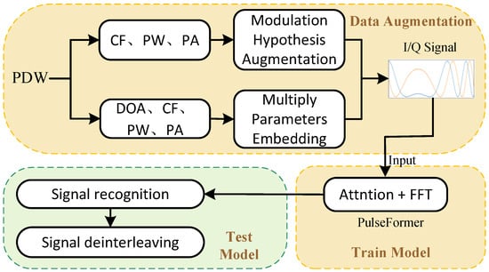
Figure 1.
The diagram of Transformer-based signal deinterleaving.
4.1. Pulse Modulation Hypothesis Data Augmentation
To obtain the discriminative features of different radar pulses more accurately, directly inputting concise PDW data into the model may not be able to fully mine the deep information of signals. Therefore, a data augmentation method is proposed to transform PDWs into more expressive intra-pulse-modulated signals. Common radar signal pulse modulation methods usually include frequency modulation, phase modulation, and hybrid modulation [31,32,33,34] etc.
- Linear frequency modulation (LFM) [31]:where A is the PA, is the CF, and represents the modulation rate of the LFM. Here, B is the signal bandwidth, and T is the PW.
- Nonlinear frequency modulation (NLFM) [32]:where is the frequency of the sine wave during the modulation process.
- Frequency-shift keying (FSK) [33]:where N represents the number of symbols within a pulse in the frequency-encoded signal, denotes the symbol width, and indicates the frequency of the nth frequency point.
- Phase-shift keying (PSK) [34]:where is the phase coding function. When is 0 and 1, the signal is a binary phase-shift keying (BPSK) signal.
In the hybrid modulation mode, three combinations of LFM-FSK, FSK-BPSK, and LFM-BPSK are considered, which increase the diversity and complexity of the signal. A random selection from these seven different modulation methods helps achieve data augmentation to better depict radar signal characteristics under different scenarios.
4.2. Multiple-Parameter Embedding
To fully dig the discriminative information from signals, multiple parameters of PDWs were embedded to further enrich the input features; we adopted the multiple-parameter embedding strategy on the modulation-hypothesis raw signals. Similar to position embedding [35], which is a common technique used in natural language processing (NLP), we expanded the fixed-length raw signal vector to a higher dimensional vector, thereby helping the model capture more discriminative features and contextual information to depict more accurate radar emitters.
Specifically, PW, PA, CF, and DOA were embedded into the raw signals by the tensor-concatenating operation to enhance discriminatory features, which can be formulated as follows:
where is obtained from intra-pulse modulation-hypothesis augmentation, x represents the parameter to be embedded, represents the dimension of the embedding vector, and i denotes the current dimension index, which varies from 0 to .
4.3. PulseFormer Network
4.3.1. Overall Architecture
In this paper, a novel PulseFormer network which integrates spectral convolutions (SP-Conv) into the classical Transformer [35] model is proposed to fully extract the local, global, and noise-resisted features of the pulses to identify the emitters. In addition, the combination of the spectral convolution layer and the self-attention layer not only helps to compensate for the sensitivity to noise of the dot product in self-attention but also solves the challenge of the multi-layer perceptron (MLP) block easily falling into local limitations [36]. The overall architecture of PulseFormer is shown in Figure 2. Based on the data preprocessing that includes pulse modulation-hypothesis data augmentation and multiple-parameter embedding, the input signal ( means the number of channels, is the feature dimension on each channel, and is the signal length along temporal dimension) is the complex-valued I/Q sequence. The normalized signal is fed to a hierarchical Transformer model with multiple stages. In each stage, i.e., stage , the input tensor ( is the feature dimension, means the number of channels, and is the signal length) is fed to a patch embedding layer and a hybrid encoder block. The patch embedding layer divides the input features into several overlapping segments and simultaneously encodes them into the feature space. The hybrid encoder block encodes the features to a higher-dimensional space with the proposed SP-Conv layer and attention mechanism. Finally, a fully connected layer maps the high-dimensional encoded features to the classes of radar emitters.
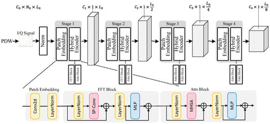
Figure 2.
The architecture of the PulseFormer model.
4.3.2. Signal Normalization
Before inputting the I/Q sequence into the model, it undergoes preprocessing, specifically amplitude normalization in terms of average power. This process can be defined as:
where is the input signal, is the normalization coefficient, represents the signal length, and denote the in-phase and quadrature components of the lth time series feature, respectively, and is the average power function applied to the input sequence.
4.3.3. Patch Embedding Layer
The patch embedding layer in Transformer aims to divide the input signal into small patches and convert them into vector representations so that the Transformer model can process these small patches and capture local and global feature information. In the ith stage, the input feature is divided into overlapping segments, learnable linear projections are carried out for each segment, and then these projections are concatenated. The embedding process is obtained.
The embedding process of this connection segment can be expressed by the following formula:
where is the learnable weight, and is the learnable bias. When , the length of the input feature is reduced by half. In the first stage, is set to match the number of channels in the corresponding dataset sample, while in other stages, .
4.3.4. Hybrid Encoder Module
In the hybrid encoder module, each stage i consists of encoder blocks. Each block includes a global-feature extraction layer and a local feature extraction layer. The global-feature extraction layer can be either an Attention (Attn) block or a Fast Fourier Transform (FFT) block, while the local feature extraction layer is an MLP layer. As illustrated in Figure 2, a Layer Normalization layer is applied before each layer, and residual connections are added before and after each layer. Formally, the hybrid encoder module can be defined as follows:
where , and represent the input and output features of the lth hybrid encoder module in the ith stage, respectively. Both the FFT block and the Attn block contain an MLP block, which is identically defined in both cases. In the following sections, we elaborate on the SP-Conv layer within the FFT block, the multi-head self-attention (MHSA) [35] within the Attn block, and the inverse residual MLP [37] block that is common to both.
SP-Conv layer. A novel SP-Conv layer is proposed in the FFT block, aiming to perform an efficient separable convolution in the spectral domain to capture noise-resisted and global features. The structure of the SP-Conv layer is shown in Figure 3a. The SP-Conv layer can be formulated as:
where and are FFT and IFFT operations, respectively, and and are pointwise and depthwise convolution, respectively, and is the tensor concatenation operation.
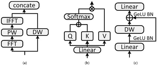
Figure 3.
Components of the PulseFormer model: (a) SP-Conv; (b) MHSA; (c) MLP.
MHSA block. The multi-layer attention mechanism used in this article is a simple original self-attention structure [35], which is illustrated in Figure 3b. The original self-attention module performs a dot product on the query and key, then applies the softmax function to obtain the normalized weight, and finally calculates the weighted sum. The formula is as follows:
where query , key , and value are obtained by a linear transformation of . is the number of patches. The symbols and are the input, key, and value dimensions, respectively. This operation is used to handle the interaction of information at different positions in the input sequence. It allows the model to distribute weights between different positions to more effectively understand the internal structure of the input sequence. Finally, several single heads are spliced together to form a multi-head attention block, which is defined as follows:
where represents the output of a single attention head as computed by Equation (15). Here, denotes the number of attention heads used in the self-attention mechanism at stage i.
MLP block. For the MLP structure, this paper uses an inverse residual feed-forward network, which looks similar to the inverted residual block [37] and is shown in Figure 3c. It has a depth-separable convolution and is composed of two parts: depthwise (DW) and pointwise (PW) convolutions. Specifically, we changed the position of the residual connection to obtain better performance.
where the GELU activation layer and batch normalization layer follow the first two layers for nonlinearization. In the MLP, the first layer expands the dimensions by 4 times, and the second layer reduces the dimensions by the same ratio. The DW convolution is beneficial for reducing computational complexity and increasing the receptive field. At the same time, similar to the classic residual network, the position of the shortcut inserted in this paper plays a key role in information retention and processing of gradient problems, thereby enhancing the training ability and feature capture performance of the network.
4.4. Loss Function
Signal deinterleaving is a typical pattern classification problem. Thus, the label-smoothed cross-entropy [38] was selected as the loss function, which is defined as follows:
where N is the number of training samples, C is the number of classes, represents the true label (typically encoded in a one-hot format), indicating whether sample i belongs to class j, and denotes the predicted probability that sample i belongs to class j.
In label-smoothing cross-entropy, the real label is no longer binary (0 or 1), but a value between 0 and 1. The form is as follows:
where is a small smoothing parameter. This operation assigns a small fraction of the probability of the real label to the other categories, reducing the model’s ability to predict one category with too much confidence and encouraging the model to consider all categories more evenly.
5. Experiment
5.1. Implementation Details
The raw I/Q signal generated by the modulation-hypothesis augmentation method on PDW data was normalized to a fixed length of 2 × 128, and the I/Q signal was expanded to 2 × 192 after the multiple-parameter embedding. The definition details of the PulseFormer is listed in Table 1, and the architecture is shown in Figure 2. We used the AdamW optimizer for training, with an initial learning rate of 0.01, a smoothing gradient parameter of (0.9, 0.99), and a weight attenuation parameter of 1 × 10⁴. The learning rate decay used the cosine annealing algorithm, and the minimum learning rate was set to 1 × 10⁵. In the experiments, each type of emitter comprised a total of 100,000 samples, which were divided into training, validation, and testing sets with a ratio of 8:1:1. The batch size when training was set to 256, and the maximum number of training epochs was 30.

Table 1.
Model definition details.
5.2. Experiments’ Setup
To validate the effectiveness of the data augmentation method and Transformer model proposed in this paper, we conducted two sets of experiments. Each set comprised nine different classes of emitters, with varying degrees of parameter overlap, which aimed to evaluate the performance of the proposed method under different overlap conditions.
In the first experiment, the nine classes of emitters had a low degree of parameter overlap. The parameters of each emitter, such as PW, CF, and DOA, had significant differences within their respective classes. The visualization of the histogram of different features is shown in Figure 4, and the details of the parameters for each emitter are provided in Table A1. In this experiment, we primarily aimed to assess the emitter classification performance of the data augmentation method and Transformer model when the parameters were distinctly separable.
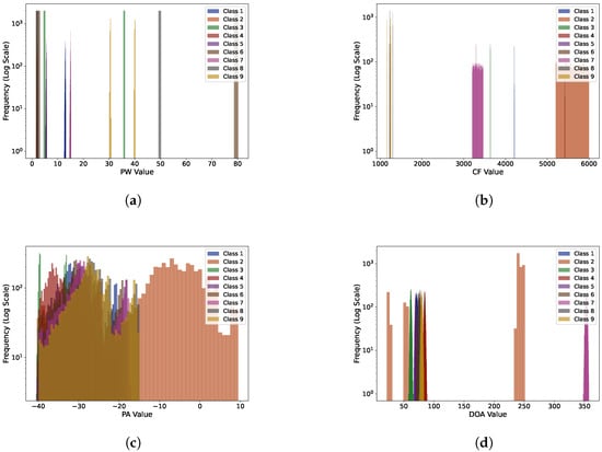
Figure 4.
Histogram visualization of different features in the first experiment: (a) PW; (b) CF; (c) PA; (d) DOA.
In the second experiment, the nine classes of emitters exhibited a high degree of parameter overlap. The parameter distributions of each emitter were closer, making the boundaries between classes more ambiguous. The histogram visualization of different features is shown in Figure 5, and the details of the parameters for each emitter are provided in Table A2. This experiment was designed to test the robustness and classification accuracy of the preprocessing method under conditions of high overlap.
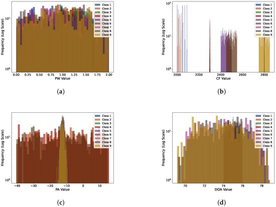
Figure 5.
Histogram visualization of different features in the second experiment: (a) PW; (b) CF; (c) PA; (d) DOA.
To comprehensively assess the accuracy of emitter identification, this paper adopted evaluation metrics such as the confusion matrix, precision, recall, and other relevant indicators. These metrics evaluated the network’s identification performance across various emitter types from multiple perspectives, ensuring a focus not only on overall identification performance but also on a detailed analysis of each emitter class’s identification accuracy. Specifically, in order to calculate Accuracy, Precision, Recall, and F1-score, four different classification outcomes for the emitter identification model were first defined:
- True Positive (TP): the number of samples correctly classified as the current class, meaning the model correctly identifies a particular type of emitter as belonging to that class.
- False Positive (FP): the number of samples from other classes that are incorrectly identified as belonging to the current class, meaning the model mistakenly classifies non-current emitter types as the current class.
- True Negative (TN): the number of samples correctly classified as belonging to other classes, meaning the model accurately categorizes non-current emitter types into their respective classes.
- False Negative (FN): the number of samples that should belong to the current class but are incorrectly classified as other classes.
Based on the four outcomes above, different evaluation metrics were calculated:
where Accuracy represents the proportion of correctly identified samples across all data points, providing an overall measure of the model’s performance. Precision, on the other hand, assesses the proportion of correctly identified samples within a predicted class, highlighting the model’s accuracy in identifying a specific class and reducing false positives. Recall measures the proportion of actual class samples that the model correctly identifies, focusing on the model’s ability to detect instances of that class and avoid missing relevant samples. The F1-score, which is the harmonic mean of Precision and Recall, provides a balanced evaluation of both the model’s Precision and Recall. It is particularly valuable when dealing with imbalanced classes, as it offers a more detailed assessment of the model’s performance.
5.3. Contribution of Modulation-Hypothesis Augmentation
The first experiment was selected to evaluate the proposed pulse modulation-hypothesis augmentation method, where we employed two distinct input modes to train the model; one was the concise PDWs, and another was I/Q signal augmentation through intra-pulse modulation hypothesis. The results for signal deinterleaving are listed in Table 2.

Table 2.
Experimental results w/w.o. modulation-hypothesis augmentation.
It can be seen that the performance of our hybrid modulation augmentation mode (marked with “Hybrid(2–7)”) was significantly boosted to a higher level compared with the concise PDW mode (marked with “PDWs”) and other single modes, and the performance gains were greatly improved from 44.01% to 44.15%. The difference between the first and second hybrid modulation modes in Table 2 is that the second mode did not include the BPSK modulation mode. Since BPSK is a form of phase modulation, where the phase alternates between 0 and π, it essentially behaves like a conventional signal. As a result, it does not provide a wealth of features that can be extracted for analysis.
5.4. Contribution of Multiple-Parameter Embedding
We evaluated the performance of multiple-parameter embedding for signal deinterleaving on the second experiment. The confusion matrices of signal deinterleaving with multiple-parameter and without multiple-parameter embedding are shown in Figure 6b and Figure 6a, respectively.
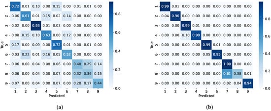
Figure 6.
The confusion matrix w/w.o. multiple-parameter embedding. (a) Modulation-hypothesis augmentation. (b) Modulation-hypothesis augmentation with multiple-parameter embedding.
It can be concluded that the multiple-parameter embedding significantly improved the classification performance in complex environments. Specifically, after multiple-parameter embedding, the classification accuracy of emitters 1, 2, 3, 4, 5, 6, 7, 8, and 9 was increased by 27%, 35%, 6%, 27%, 27%, 43%, 60%, 2%, and 50%, respectively. Additionally, as shown in the t-SNE visualization in Figure 7, the method using multiple-parameter embedding demonstrated a higher discriminative ability compared to when it was not used, which was consistent with the confusion matrix results shown in Figure 6. However, the confusion matrix revealed that the misclassification between the seventh and eighth classes was mainly due to the fact that the parameter ranges of the eighth class’s signal overlapped with those of the seventh class. For example, the carrier frequency range of the seventh class was 2799∼2800 Hz, while the eighth class covered a broader range of 2795∼2805 Hz. As a result, many data points from the seventh class were misclassified into the eighth class. This issue is unavoidable because of the significant overlap in parameters between the two classes. We will further explore strategies to improve the classification model to better handle such overlaps.
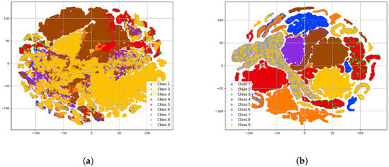
Figure 7.
The t-SNE visualization shows the high-dimensional feature distribution predicted by our model under the modulation-hypothesis augmentation methods. (a) Without multiple-parameter embedding. (b) With multiple-parameter embedding.
6. Discussion
6.1. Experiments
To validate the advantages of our method compared to other methods, we conducted three sets of experiments. The parameters for these experiments were consistent with those in the literature [4]. The details of the parameters for each emitter are provided in Table 3.

Table 3.
Emitter settings in experiments 1–3.
In addition, the pulse parameters followed the rule of , where is the duty cycle. Furthermore, PRI, PW, and RF exhibited various modulation types, such as constant, dwell and switch (D&S), and staggered. These modulation modes configured with different PRI values offered diverse pulse trains for different emitters. Three groups of experiment settings were configured. Experiment 1 aimed to check different PRI modulation types with similar intra-pulse parameters, and experiment 2 aimed to validate two types of PRI modulation with similar intra-pulse parameters. Experiment 3 aimed to validate the extremely similar PRI modulation mode with similar intra-pulse parameters. In addition, the issue of target pulse loss and the presence of random noise pulses in the intercepted pulse stream was considered. The target pulse loss rate was denoted by , while represented the noise-to-target ratio, defined as the ratio of the number of noise pulses in the intercepted pulse train to the average number of pulses from each radar emitter. Thus, in the three experiments mentioned above, the values of and for each training data sample were randomly selected within the range of and .
6.2. Comparison with Previous Methods
SDIF [6] and PRI-Tran [7] are classic traditional methods in signal deinterleaving that have been taken as baseline and compared in several previous studies. Additionally, there are few deep learning methods for signal deinterleaving from single pulse, and most are from pulse trains, which rely on the PRI, so BLSTM [4] and BGRU [4] were the rare comparable approach with our method. The overall performance of previous methods and our method with the three experimental settings were evaluated, and the results are listed in Table 4.

Table 4.
Comparison with previous methods.
It can be concluded that our method achieved state-of-the-art performance on accuracy and obtained 6.4–33.4% accuracy gains compared with traditional methods, such as SDIF [6] and PRI-Tran [7] on experiments 1 and 2, respectively. In addition, compared with other neural network methods, such as BLSTM [4] and BGRU [4], our PulseFormer obtained 2.9–5.8% accuracy gains on experiments 1 and 2, respectively. Moreover, from experiment 3, it can be seen that our PulseFormer was able to effectively discriminate among those similar pulses, which were probably from a heavy overlap of parameters, and relied on pulse trains and PRI parameters. However, previous methods such as BLSTM [4], BGRU [4], SDIF [6], and PRI-Tran [7] were not competent for these complex scenarios. The reason why BLSTM [4], BGRU [4], SDIF [6], and PRI Tran [7] could not be applied to these complex scenarios is because these algorithms rely on the PRI of emitters for signal deinterleaving. When the ranges of the PRI parameters heavily overlap or the modulation types are completely similar, it is difficult to distinguish these emitters. Our proposed method, utilizing intra-pulse parameters and advanced deep learning models for signal deinterleaving, achieved more satisfactory results. In the future, we will explore how to combine inter-pulse and intra-pulse parameters to obtain a more reliable signal deinterleaving method.
6.3. Analysis under Different Noise Conditions
Furthermore, we evaluated those methods on experiment 1 under different noise conditions, where the noise coefficient (noise-to-target ratio) was from 0 to 0.25, and the result is shown in Figure 8.
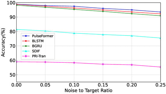
Figure 8.
Performance comparison under different noise conditions.
It can be seen that the proposed PulseFormer showed better performance to resist noise. Initially, at zero noise ratio, the overall performance of the method slightly exceeded the next best model (i.e., BLSTM [4]) by 0.2%. However, as the noise ratio increased to 0.25, the accuracy of our method demonstrated a notable improvement of 1.3% compared with the BLSTM method. The BLSTM [4] and BGRU [4] methods rely on inter-pulse sequences, emphasizing the order in which the receiver captures the pulses from various radar emitters. Consequently, when there is an excessive number of noise pulses, the accuracy of these methods declines rapidly. In contrast, the approach proposed in this work leverages intra-pulse parameters, making it less sensitive to noise. Furthermore, the results indicated that as increased, the number of noise pulses increased relative to the number of target signals, making it more challenging for the model to distinguish between valid signals and noise pulses. In a lower signal-to-noise ratio (SNR), the results introduce greater ambiguity during the classification process and ultimately lead to a degradation in accuracy.
6.4. Analysis under Different Pulse Loss Rates
Finally, we evaluated those methods on experiment 1 under different pulse loss rates, where (pulse loss rate) was varied from 0 to 0.25, and the result is shown in Figure 9.
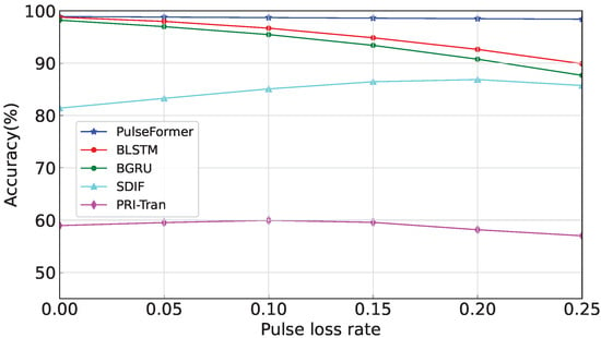
Figure 9.
Performance comparison under pulse loss.
It can be seen that the proposed PulseFormer showed better performance to resist pulse loss. Initially, at zero noise ratio, the overall performance of the method slightly exceeded the next best model (i.e., BLSTM [4]) by 0.2%. However, as the pulse loss ratio increased to 0.25, the accuracy of our method demonstrated a notable improvement of 8.51% compared with the BLSTM method. Overall, pulse loss did not affect the performance of our method. This robustness was attributed to the fact that the proposed method did not rely on inter-pulse parameters. In contrast, the BLSTM [4] and BGRU [4] methods were heavily dependent on the inter-pulse parameter DTOA, making them vulnerable to disruptions caused by pulse loss. Consequently, the loss of pulses interfered with the receiver’s ability to accurately sequence the emitter signals, leading to a decrease in accuracy.
7. Conclusions
In this paper, we proposed a multi-parameter deep learning method for radar signal deinterleaving, which could achieve better performance in more complex scenarios with a single PDW parameter and without relying on PRI parameters. The modulation-hypothesis data augmentation, multiple-parameter embedding, and spectral convolution-enhanced Transformer model were proposed for this issue. Experimental results on synthesized data showed that our method outperformed most previous methods.
Author Contributions
Conceptualization, H.L. and L.W.; methodology, H.L.; software, L.W.; validation, L.W. and H.L.; formal analysis, G.W.; investigation, G.W.; resources, G.W.; data curation, L.W.; writing—original draft preparation, L.W.; writing—review and editing, H.L.; visualization, L.W.; supervision, H.L.; project administration, H.L.; funding acquisition, H.L. All authors have read and agreed to the published version of the manuscript.
Funding
This research received no external funding.
Data Availability Statement
Not applicable.
Conflicts of Interest
The authors declare no conflicts of interest.
Abbreviations
The following abbreviations are used in this manuscript:
| PDW | Pulse description word |
| PRI | Pulse repetition interval |
| CF | Carrier frequency |
| PW | Pulse width |
| PA | Pulse amplitude |
| DOA | Direction of arrival |
| TOA | Time of arrival |
| LSTM | Long short-term memory |
| LFM | Linear frequency modulation |
| NLFM | Nonlinear frequency modulation |
| FSK | Frequency-shift keying |
| PSK | Phase-shift keying |
| NLP | Natural language processing |
| MLP | Multi-layer perceptron |
| SP-Conv | Spectral convolution |
| MHSA | Multi-head self-attention |
Appendix A

Table A1.
Emitter settings in the first experiment.
Table A1.
Emitter settings in the first experiment.
| Radar | PW/µs | CF/MHz | PA/dB | DOA/° | Modulation Type |
|---|---|---|---|---|---|
| 1 | 12.5∼13.2 | 4208∼4211 | −40∼−20.5 | 68∼75 | PSK |
| 2 | 1.5∼2.2 | 5200∼6000 | −40∼9 | 21∼251 | NLFM |
| 3 | 4.5∼36.2 | 3635∼3639 | −40∼−33 | 57∼66 | NLFM |
| 4 | 1.5∼2.4 | 5416∼5420 | −40∼−25 | 82∼89 | LFM-BPSK |
| 5 | 5∼6 | 3293∼3297 | −44∼−18 | 66∼73 | LFM |
| 6 | 1.5∼80 | 1223∼1231 | −40∼−19 | 70∼78 | LFM-FSK |
| 7 | 14.5∼15.2 | 3200∼3470 | −40∼−18 | 350∼358 | NLFM |
| 8 | 1.5∼51 | 1228∼1302 | −40∼−15 | 73∼81 | FSK-BPSK |
| 9 | 30∼41 | 1158∼1267 | −40∼−16 | 75∼82 | FSK |

Table A2.
Emitter settings in the second experiment.
Table A2.
Emitter settings in the second experiment.
| Radar | PW/µs | CF/MHz | PA/dB | DOA/° | Modulation Type |
|---|---|---|---|---|---|
| 1 | 0∼2 | 2000∼2090 | −17∼−7 | 74∼76 | FSK |
| 2 | 0∼2 | 2000∼2040 | −40∼16 | 74∼76 | FSK |
| 3 | 0∼2 | 2295∼2305 | −17∼−7 | 74∼76 | LFM |
| 4 | 0∼2 | 2295∼2305 | −40∼16 | 74∼76 | LFM |
| 5 | 0∼2 | 2400∼2500 | −17∼−7 | 74∼76 | NLFM |
| 6 | 0∼2 | 2450∼2500 | −40∼16 | 74∼76 | NLFM |
| 7 | 0∼2 | 2799∼2800 | −17∼−7 | 69∼79 | LFM |
| 8 | 0∼2 | 2795∼2805 | −17∼−7 | 69∼79 | NLFM |
| 9 | 0∼2 | 2750∼2850 | −17∼−7 | 69∼79 | NLFM |
References
- Liu, Z.-M.; Philip, S.Y. Classification, denoising, and deinterleaving of pulse streams with recurrent neural networks. IEEE Trans. Aerosp. Electron. Syst. 2018, 55, 1624–1639. [Google Scholar] [CrossRef]
- Jiang, H.; Pang, Z.; Tang, P.; Jia, L. Intrapulse modulation recognition based on pulse description words. In Proceedings of the 2013 6th International Congress on Image and Signal Processing (CISP), Hangzhou, China, 16–18 December 2013; Volume 3, pp. 1367–1371. [Google Scholar]
- Wu, B.; Yuan, S.; Li, P.; Jing, Z.; Huang, S.; Zhao, Y. Radar emitter signal recognition based on one-dimensional convolutional neural network with attention mechanism. Sensors 2020, 20, 6350. [Google Scholar] [CrossRef] [PubMed]
- Chao, W.; Sun, L.; Liu, Z.; Huang, Z. A radar signal deinterleaving method based on semantic segmentation with neural network. IEEE Trans. Signal Process. 2022, 70, 5806–5821. [Google Scholar] [CrossRef]
- Mardia, H. New techniques for the deinterleaving of repetitive sequences. IEE Proc. F Radar Signal Process. 1989, 136, 149–154. [Google Scholar] [CrossRef]
- Milojević, D.; Popović, B.M. Improved algorithm for the deinterleaving of radar pulses. IEE Proc. 1992, 139, 98–104. [Google Scholar]
- Nishiguchi, K.; Kobayashi, M. Improved algorithm for estimating pulse repetition intervals. IEEE Trans. Aerosp. Electron. Syst. 2000, 36, 407–421. [Google Scholar] [CrossRef]
- Niranjan, R.; Rao, C.R.; Singh, A. Real-time identification of exotic modulated radar signals for electronic intelligence systems. In Proceedings of the 2021 Emerging Trends in Industry 4.0 (ETI 4.0), Raigarh, India, 19–21 May 2021; pp. 1–4. [Google Scholar]
- Yuan, S.; Wu, B.; Li, P. Intra-pulse modulation classification of radar emitter signals based on a 1-d selective kernel convolutional neural network. Remote Sens. 2021, 13, 2799. [Google Scholar] [CrossRef]
- Zhang, Y.; Zhou, Z.; Li, X. Specific emitter identification handling modulation variation with margin disparity discrepancy. arXiv 2024, arXiv:2403.11531. [Google Scholar]
- Su, H.; Fan, X.; Liu, H. Robust and efficient modulation recognition with pyramid signal transformer. In Proceedings of the GLOBECOM 2022—2022 IEEE Global Communications Conference, Rio de Janeiro, Brazil, 4–8 December 2022; pp. 1868–1874. [Google Scholar]
- Fan, X.; Liu, H. Flexformer: Flexible transformer for efficient visual recognition. Pattern Recognit. Lett. 2023, 169, 95–101. [Google Scholar] [CrossRef]
- Moore, J.B.; Krishnamurthy, V. Deinterleaving pulse trains using discrete-time stochastic dynamic-linear models. IEEE Trans. Signal Process. 1994, 42, 3092–3103. [Google Scholar] [CrossRef]
- Conroy, T.; Moore, J.B. The limits of extended kalman filtering for pulse train deinterleaving. IEEE Trans. Signal Process. 1998, 46, 3326–3332. [Google Scholar] [CrossRef]
- Visnevski, N.; Haykin, S.; Krishnamurthy, V.; Dilkes, F.A.; Lavoie, P. Hidden markov models for radar pulse train analysis in electronic warfare. In Proceedings of the IEEE International Conference on Acoustics, Speech, and Signal Processing, Philadelphia, PA, USA, 23 March 2005; Volume 5, p. 597. [Google Scholar]
- Logothetis, A.; Krishnamurthy, V. An interval-amplitude algorithm for deinterleaving stochastic pulse train sources. IEEE Trans. Signal Process. 1998, 46, 1344–1350. [Google Scholar] [CrossRef]
- Xu, T.; Yuan, S.; Liu, Z.; Guo, F. Radar emitter recognition based on parameter set clustering and classification. Remote Sens. 2022, 14, 4468. [Google Scholar] [CrossRef]
- Al-Malahi, A.; Almaqtari, O.; Ayedh, W.; Tang, B. Radar signal sorting using combined residual and recurrent neural network (CRRNN). In Proceedings of the 2021 18th International Computer Conference on Wavelet Active Media Technology and Information Processing (ICCWAMTIP), Chengdu, China, 17–19 December 2021; pp. 21–27. [Google Scholar]
- Al-Malahi, A.; Farhan, A.; Feng, H.; Almaqtari, O.; Tang, B. An intelligent radar signal classification and deinterleaving method with unified residual recurrent neural network. IET Radar Sonar Navig. 2023, 17, 1259–1276. [Google Scholar] [CrossRef]
- Nuhoglu, M.A.; Alp, Y.K.; Ulusoy, M.E.C.; Çırpan, H.A. Image segmentation for radar signal deinterleaving using deep learning. IEEE Trans. Aerosp. Electron. Syst. 2023, 59, 541–554. [Google Scholar] [CrossRef]
- Luo, Y.; Liu, T.; Li, X.; Liu, H. A cross-domain radar emitter recognition method with few-shot learning. In Proceedings of the 2023 4th International Symposium on Computer Engineering and Intelligent Communications (ISCEIC), Nanjing, China, 18–20 August 2023; pp. 476–482. [Google Scholar]
- Xiang, H.; Shen, F.; Zhao, J. Deep toa mask-based recursive radar pulse deinterleaving. IEEE Trans. Aerosp. Electron. Syst. 2023, 59, 989–1006. [Google Scholar] [CrossRef]
- Scherreik, M.; Rigling, B. Clustering radar pulses with bayesian nonparametrics: A case for online processing. In Proceedings of the 2020 IEEE International Radar Conference, Washington, DC, USA, 28–30 April 2020; pp. 1052–1057. [Google Scholar]
- Mottier, M.; Chardon, G.; Pascal, F. Deinterleaving and clustering unknown radar pulses. In Proceedings of the 2021 IEEE Radar Conference, Atlanta, GA, USA, 7–14 May 2021; pp. 1–6. [Google Scholar]
- Dong, X.; Liang, Y.; Wang, J. Distributed clustering method based on spatial information. IEEE Access 2022, 10, 53143–53152. [Google Scholar] [CrossRef]
- Li, H.; Zhao, J.; Zhang, Y. Signals deinterleaving for es systems using improved CFSFDP algorithm. In Proceedings of the 2019 IEEE Radar Conference, Boston, MA, USA, 22–26 April 2019; pp. 1–5. [Google Scholar]
- Mu, H.; Gu, J.; Zhao, Y. A deinterleaving method for mixed pulse signals in complex electromagnetic environment. In Proceedings of the 2019 International Conference on Control, Automation and Information Sciences (ICCAIS), Chengdu, China, 23–26 October 2019; pp. 1–4. [Google Scholar]
- Kang, Z.; Zhong, Y.; Wu, Y.; Cai, Y. Signal deinterleaving based on u-net networks. In Proceedings of the 2023 8th International Conference on Computer and Communication Systems (ICCCS), Guangzhou, China, 21–23 April 2023; pp. 62–67. [Google Scholar]
- Mei, J.; Li, C.; Cao, Y.; Wang, X.; Liu, Z. Radar signal sorting based on image semantic segmentation. J. Phys. Conf. Ser. 2024, 2807, 012036. [Google Scholar] [CrossRef]
- Luo, Z.; Wang, X.; Yuan, S.; Liu, Z. Radar emitter recognition based on spiking neural networks. Remote Sens. 2024, 16, 2680. [Google Scholar] [CrossRef]
- Ben, G.; Zheng, X.; Wang, Y.; Zhang, X.; Zhang, N. Chirp signal denoising based on convolution neural network. Circuits Syst. Signal Process. 2021, 40, 5468–5482. [Google Scholar] [CrossRef]
- Leśnik, C. Nonlinear frequency modulated signal design. Acta Phys. Pol. A 2009, 116, 351–354. [Google Scholar] [CrossRef]
- Faruque, S. Frequency shift keying (FSK). In Free Space Laser Communication with Ambient Light Compensation; Springer: Berlin/Heidelberg, Germany, 2021; pp. 189–200. [Google Scholar]
- Faruque, S. Phase shift keying (PSK). In Free Space Laser Communication with Ambient Light Compensation; Springer: Berlin/Heidelberg, Germany, 2021; pp. 201–215. [Google Scholar]
- Vaswani, A. Attention is all you need. arXiv 2017, arXiv:1706.03762. [Google Scholar]
- Patro, B.N.; Namboodiri, V.P.; Agneeswaran, V.S. Spectformer: Frequency and attention is what you need in a vision transformer. arXiv 2023, arXiv:2304.06446. [Google Scholar]
- Sandler, M.; Howard, A.; Zhu, M.; Zhmoginov, A.; Chen, L.-C. Mobilenetv2: Inverted residuals and linear bottlenecks. In Proceedings of the IEEE conference on computer vision and pattern recognition, Salt Lake City, UT, USA, 18–23 June 2018; pp. 4510–4520. [Google Scholar]
- Müller, R.; Kornblith, S.; Hinton, G.E. When does label smoothing help? In Proceedings of the NIPS’19: 33rd International Conference on Neural Information Processing Systems, Vancouver, BC, Canada, 8–14 December 2019; p. 32. [Google Scholar]
Disclaimer/Publisher’s Note: The statements, opinions and data contained in all publications are solely those of the individual author(s) and contributor(s) and not of MDPI and/or the editor(s). MDPI and/or the editor(s) disclaim responsibility for any injury to people or property resulting from any ideas, methods, instructions or products referred to in the content. |
© 2024 by the authors. Licensee MDPI, Basel, Switzerland. This article is an open access article distributed under the terms and conditions of the Creative Commons Attribution (CC BY) license (https://creativecommons.org/licenses/by/4.0/).