
Emitter Signal Deinterleaving Based on Single PDW with Modulation-Hypothesis-Augmented Transformer


Abstract
1. Introduction
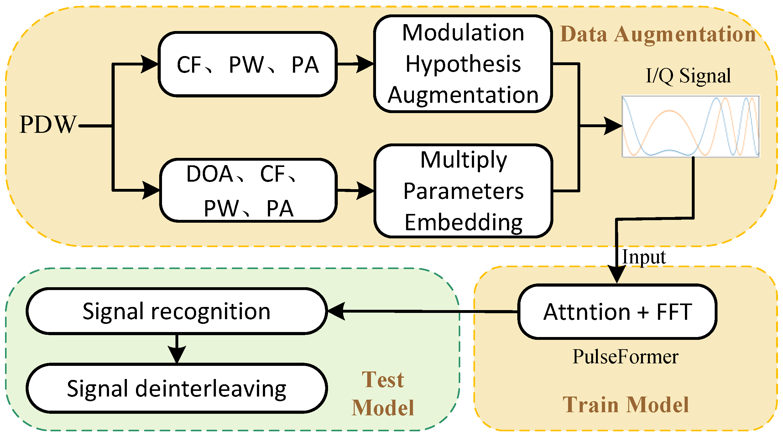
- A data augmentation mechanism based on a modulation hypothesis of intra-pulse parameters is proposed to generate rich I/Q signals from a single PDW.
- An embedding method based on multiply parameters is proposed to enrich the emitter information to achieve more reliable signal deinterleaving.
- A spectral convolution-enhanced Transformer model based on local, global, and a noise-resisted feature representation learning mechanism is built for signal classification.
- Experimental results show that our method achieves state-of-the-art performance compared with previous methods without relying on PRI parameters.
2. Related Work
2.1. TOA-Based Deinterleaving Methods
2.2. Multi-Parameter-Based Deinterleaving Methods
3. Radar Emitter Signal Deinterleaving Problem Description
4. Our Method
4.1. Pulse Modulation Hypothesis Data Augmentation
- Linear frequency modulation (LFM) [31]:where A is the PA, is the CF, and represents the modulation rate of the LFM. Here, B is the signal bandwidth, and T is the PW.
- Nonlinear frequency modulation (NLFM) [32]:where is the frequency of the sine wave during the modulation process.
- Frequency-shift keying (FSK) [33]:where N represents the number of symbols within a pulse in the frequency-encoded signal, denotes the symbol width, and indicates the frequency of the nth frequency point.
- Phase-shift keying (PSK) [34]:where is the phase coding function. When is 0 and 1, the signal is a binary phase-shift keying (BPSK) signal.
4.2. Multiple-Parameter Embedding
4.3. PulseFormer Network
4.3.1. Overall Architecture
4.3.2. Signal Normalization
4.3.3. Patch Embedding Layer
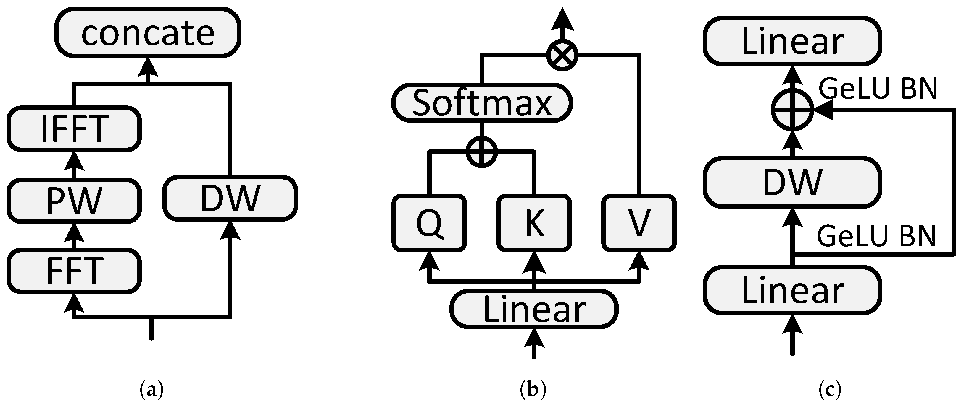
4.3.4. Hybrid Encoder Module
4.4. Loss Function
5. Experiment
5.1. Implementation Details
5.2. Experiments’ Setup
- True Positive (TP): the number of samples correctly classified as the current class, meaning the model correctly identifies a particular type of emitter as belonging to that class.
- False Positive (FP): the number of samples from other classes that are incorrectly identified as belonging to the current class, meaning the model mistakenly classifies non-current emitter types as the current class.
- True Negative (TN): the number of samples correctly classified as belonging to other classes, meaning the model accurately categorizes non-current emitter types into their respective classes.
- False Negative (FN): the number of samples that should belong to the current class but are incorrectly classified as other classes.
5.3. Contribution of Modulation-Hypothesis Augmentation
5.4. Contribution of Multiple-Parameter Embedding
6. Discussion
6.1. Experiments
6.2. Comparison with Previous Methods
6.3. Analysis under Different Noise Conditions
6.4. Analysis under Different Pulse Loss Rates
7. Conclusions
Author Contributions
Funding
Data Availability Statement
Conflicts of Interest
Abbreviations
| PDW | Pulse description word |
| PRI | Pulse repetition interval |
| CF | Carrier frequency |
| PW | Pulse width |
| PA | Pulse amplitude |
| DOA | Direction of arrival |
| TOA | Time of arrival |
| LSTM | Long short-term memory |
| LFM | Linear frequency modulation |
| NLFM | Nonlinear frequency modulation |
| FSK | Frequency-shift keying |
| PSK | Phase-shift keying |
| NLP | Natural language processing |
| MLP | Multi-layer perceptron |
| SP-Conv | Spectral convolution |
| MHSA | Multi-head self-attention |
Appendix A

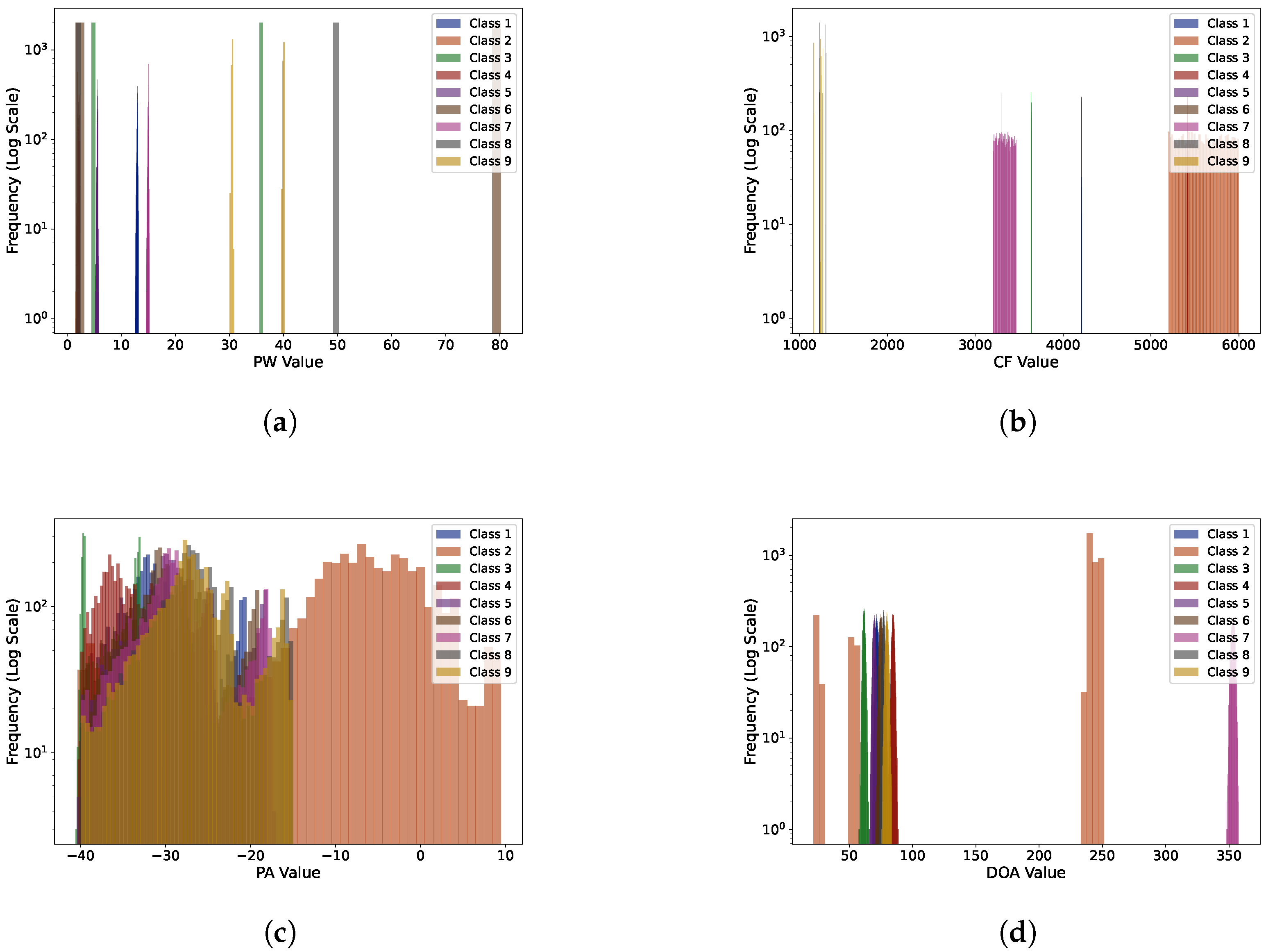
| Radar | PW/µs | CF/MHz | PA/dB | DOA/° | Modulation Type |
|---|---|---|---|---|---|
| 1 | 12.5∼13.2 | 4208∼4211 | −40∼−20.5 | 68∼75 | PSK |
| 2 | 1.5∼2.2 | 5200∼6000 | −40∼9 | 21∼251 | NLFM |
| 3 | 4.5∼36.2 | 3635∼3639 | −40∼−33 | 57∼66 | NLFM |
| 4 | 1.5∼2.4 | 5416∼5420 | −40∼−25 | 82∼89 | LFM-BPSK |
| 5 | 5∼6 | 3293∼3297 | −44∼−18 | 66∼73 | LFM |
| 6 | 1.5∼80 | 1223∼1231 | −40∼−19 | 70∼78 | LFM-FSK |
| 7 | 14.5∼15.2 | 3200∼3470 | −40∼−18 | 350∼358 | NLFM |
| 8 | 1.5∼51 | 1228∼1302 | −40∼−15 | 73∼81 | FSK-BPSK |
| 9 | 30∼41 | 1158∼1267 | −40∼−16 | 75∼82 | FSK |
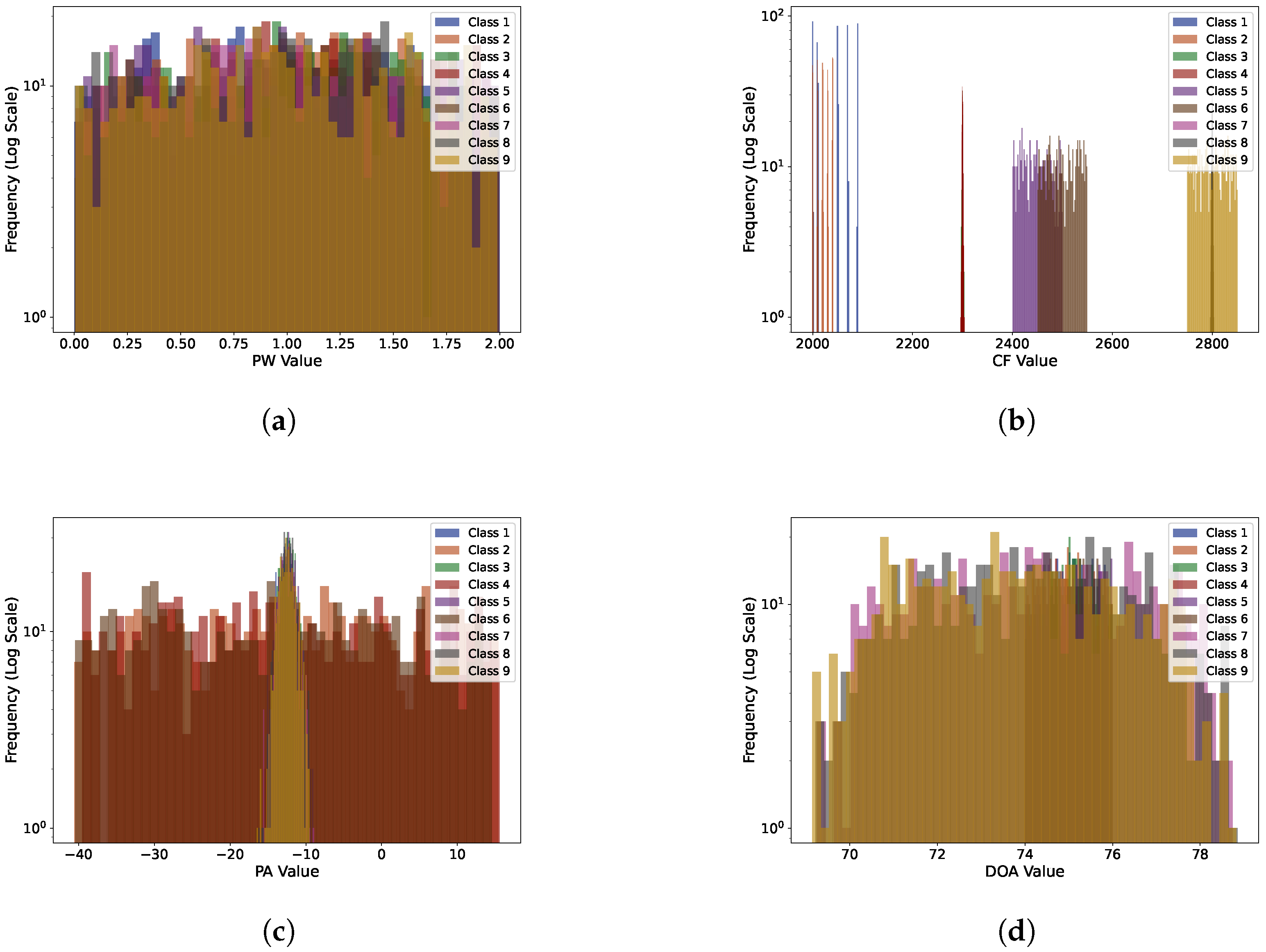
| Radar | PW/µs | CF/MHz | PA/dB | DOA/° | Modulation Type |
|---|---|---|---|---|---|
| 1 | 0∼2 | 2000∼2090 | −17∼−7 | 74∼76 | FSK |
| 2 | 0∼2 | 2000∼2040 | −40∼16 | 74∼76 | FSK |
| 3 | 0∼2 | 2295∼2305 | −17∼−7 | 74∼76 | LFM |
| 4 | 0∼2 | 2295∼2305 | −40∼16 | 74∼76 | LFM |
| 5 | 0∼2 | 2400∼2500 | −17∼−7 | 74∼76 | NLFM |
| 6 | 0∼2 | 2450∼2500 | −40∼16 | 74∼76 | NLFM |
| 7 | 0∼2 | 2799∼2800 | −17∼−7 | 69∼79 | LFM |
| 8 | 0∼2 | 2795∼2805 | −17∼−7 | 69∼79 | NLFM |
| 9 | 0∼2 | 2750∼2850 | −17∼−7 | 69∼79 | NLFM |
References
- Liu, Z.-M.; Philip, S.Y. Classification, denoising, and deinterleaving of pulse streams with recurrent neural networks. IEEE Trans. Aerosp. Electron. Syst. 2018, 55, 1624–1639. [Google Scholar] [CrossRef]
- Jiang, H.; Pang, Z.; Tang, P.; Jia, L. Intrapulse modulation recognition based on pulse description words. In Proceedings of the 2013 6th International Congress on Image and Signal Processing (CISP), Hangzhou, China, 16–18 December 2013; Volume 3, pp. 1367–1371. [Google Scholar]
- Wu, B.; Yuan, S.; Li, P.; Jing, Z.; Huang, S.; Zhao, Y. Radar emitter signal recognition based on one-dimensional convolutional neural network with attention mechanism. Sensors 2020, 20, 6350. [Google Scholar] [CrossRef] [PubMed]
- Chao, W.; Sun, L.; Liu, Z.; Huang, Z. A radar signal deinterleaving method based on semantic segmentation with neural network. IEEE Trans. Signal Process. 2022, 70, 5806–5821. [Google Scholar] [CrossRef]
- Mardia, H. New techniques for the deinterleaving of repetitive sequences. IEE Proc. F Radar Signal Process. 1989, 136, 149–154. [Google Scholar] [CrossRef]
- Milojević, D.; Popović, B.M. Improved algorithm for the deinterleaving of radar pulses. IEE Proc. 1992, 139, 98–104. [Google Scholar]
- Nishiguchi, K.; Kobayashi, M. Improved algorithm for estimating pulse repetition intervals. IEEE Trans. Aerosp. Electron. Syst. 2000, 36, 407–421. [Google Scholar] [CrossRef]
- Niranjan, R.; Rao, C.R.; Singh, A. Real-time identification of exotic modulated radar signals for electronic intelligence systems. In Proceedings of the 2021 Emerging Trends in Industry 4.0 (ETI 4.0), Raigarh, India, 19–21 May 2021; pp. 1–4. [Google Scholar]
- Yuan, S.; Wu, B.; Li, P. Intra-pulse modulation classification of radar emitter signals based on a 1-d selective kernel convolutional neural network. Remote Sens. 2021, 13, 2799. [Google Scholar] [CrossRef]
- Zhang, Y.; Zhou, Z.; Li, X. Specific emitter identification handling modulation variation with margin disparity discrepancy. arXiv 2024, arXiv:2403.11531. [Google Scholar]
- Su, H.; Fan, X.; Liu, H. Robust and efficient modulation recognition with pyramid signal transformer. In Proceedings of the GLOBECOM 2022—2022 IEEE Global Communications Conference, Rio de Janeiro, Brazil, 4–8 December 2022; pp. 1868–1874. [Google Scholar]
- Fan, X.; Liu, H. Flexformer: Flexible transformer for efficient visual recognition. Pattern Recognit. Lett. 2023, 169, 95–101. [Google Scholar] [CrossRef]
- Moore, J.B.; Krishnamurthy, V. Deinterleaving pulse trains using discrete-time stochastic dynamic-linear models. IEEE Trans. Signal Process. 1994, 42, 3092–3103. [Google Scholar] [CrossRef]
- Conroy, T.; Moore, J.B. The limits of extended kalman filtering for pulse train deinterleaving. IEEE Trans. Signal Process. 1998, 46, 3326–3332. [Google Scholar] [CrossRef]
- Visnevski, N.; Haykin, S.; Krishnamurthy, V.; Dilkes, F.A.; Lavoie, P. Hidden markov models for radar pulse train analysis in electronic warfare. In Proceedings of the IEEE International Conference on Acoustics, Speech, and Signal Processing, Philadelphia, PA, USA, 23 March 2005; Volume 5, p. 597. [Google Scholar]
- Logothetis, A.; Krishnamurthy, V. An interval-amplitude algorithm for deinterleaving stochastic pulse train sources. IEEE Trans. Signal Process. 1998, 46, 1344–1350. [Google Scholar] [CrossRef]
- Xu, T.; Yuan, S.; Liu, Z.; Guo, F. Radar emitter recognition based on parameter set clustering and classification. Remote Sens. 2022, 14, 4468. [Google Scholar] [CrossRef]
- Al-Malahi, A.; Almaqtari, O.; Ayedh, W.; Tang, B. Radar signal sorting using combined residual and recurrent neural network (CRRNN). In Proceedings of the 2021 18th International Computer Conference on Wavelet Active Media Technology and Information Processing (ICCWAMTIP), Chengdu, China, 17–19 December 2021; pp. 21–27. [Google Scholar]
- Al-Malahi, A.; Farhan, A.; Feng, H.; Almaqtari, O.; Tang, B. An intelligent radar signal classification and deinterleaving method with unified residual recurrent neural network. IET Radar Sonar Navig. 2023, 17, 1259–1276. [Google Scholar] [CrossRef]
- Nuhoglu, M.A.; Alp, Y.K.; Ulusoy, M.E.C.; Çırpan, H.A. Image segmentation for radar signal deinterleaving using deep learning. IEEE Trans. Aerosp. Electron. Syst. 2023, 59, 541–554. [Google Scholar] [CrossRef]
- Luo, Y.; Liu, T.; Li, X.; Liu, H. A cross-domain radar emitter recognition method with few-shot learning. In Proceedings of the 2023 4th International Symposium on Computer Engineering and Intelligent Communications (ISCEIC), Nanjing, China, 18–20 August 2023; pp. 476–482. [Google Scholar]
- Xiang, H.; Shen, F.; Zhao, J. Deep toa mask-based recursive radar pulse deinterleaving. IEEE Trans. Aerosp. Electron. Syst. 2023, 59, 989–1006. [Google Scholar] [CrossRef]
- Scherreik, M.; Rigling, B. Clustering radar pulses with bayesian nonparametrics: A case for online processing. In Proceedings of the 2020 IEEE International Radar Conference, Washington, DC, USA, 28–30 April 2020; pp. 1052–1057. [Google Scholar]
- Mottier, M.; Chardon, G.; Pascal, F. Deinterleaving and clustering unknown radar pulses. In Proceedings of the 2021 IEEE Radar Conference, Atlanta, GA, USA, 7–14 May 2021; pp. 1–6. [Google Scholar]
- Dong, X.; Liang, Y.; Wang, J. Distributed clustering method based on spatial information. IEEE Access 2022, 10, 53143–53152. [Google Scholar] [CrossRef]
- Li, H.; Zhao, J.; Zhang, Y. Signals deinterleaving for es systems using improved CFSFDP algorithm. In Proceedings of the 2019 IEEE Radar Conference, Boston, MA, USA, 22–26 April 2019; pp. 1–5. [Google Scholar]
- Mu, H.; Gu, J.; Zhao, Y. A deinterleaving method for mixed pulse signals in complex electromagnetic environment. In Proceedings of the 2019 International Conference on Control, Automation and Information Sciences (ICCAIS), Chengdu, China, 23–26 October 2019; pp. 1–4. [Google Scholar]
- Kang, Z.; Zhong, Y.; Wu, Y.; Cai, Y. Signal deinterleaving based on u-net networks. In Proceedings of the 2023 8th International Conference on Computer and Communication Systems (ICCCS), Guangzhou, China, 21–23 April 2023; pp. 62–67. [Google Scholar]
- Mei, J.; Li, C.; Cao, Y.; Wang, X.; Liu, Z. Radar signal sorting based on image semantic segmentation. J. Phys. Conf. Ser. 2024, 2807, 012036. [Google Scholar] [CrossRef]
- Luo, Z.; Wang, X.; Yuan, S.; Liu, Z. Radar emitter recognition based on spiking neural networks. Remote Sens. 2024, 16, 2680. [Google Scholar] [CrossRef]
- Ben, G.; Zheng, X.; Wang, Y.; Zhang, X.; Zhang, N. Chirp signal denoising based on convolution neural network. Circuits Syst. Signal Process. 2021, 40, 5468–5482. [Google Scholar] [CrossRef]
- Leśnik, C. Nonlinear frequency modulated signal design. Acta Phys. Pol. A 2009, 116, 351–354. [Google Scholar] [CrossRef]
- Faruque, S. Frequency shift keying (FSK). In Free Space Laser Communication with Ambient Light Compensation; Springer: Berlin/Heidelberg, Germany, 2021; pp. 189–200. [Google Scholar]
- Faruque, S. Phase shift keying (PSK). In Free Space Laser Communication with Ambient Light Compensation; Springer: Berlin/Heidelberg, Germany, 2021; pp. 201–215. [Google Scholar]
- Vaswani, A. Attention is all you need. arXiv 2017, arXiv:1706.03762. [Google Scholar]
- Patro, B.N.; Namboodiri, V.P.; Agneeswaran, V.S. Spectformer: Frequency and attention is what you need in a vision transformer. arXiv 2023, arXiv:2304.06446. [Google Scholar]
- Sandler, M.; Howard, A.; Zhu, M.; Zhmoginov, A.; Chen, L.-C. Mobilenetv2: Inverted residuals and linear bottlenecks. In Proceedings of the IEEE conference on computer vision and pattern recognition, Salt Lake City, UT, USA, 18–23 June 2018; pp. 4510–4520. [Google Scholar]
- Müller, R.; Kornblith, S.; Hinton, G.E. When does label smoothing help? In Proceedings of the NIPS’19: 33rd International Conference on Neural Information Processing Systems, Vancouver, BC, Canada, 8–14 December 2019; p. 32. [Google Scholar]


| Feature Map | Layer Name | Size of Parameter | |
|---|---|---|---|
| Stage1 | Patch embedding | ||
| Hybrid encoder | |||
| Stage2 | Patch embedding | ||
| Hybrid encoder | |||
| Stage3 | Patch embedding | ||
| Hybrid encoder | |||
| Stage4 | Patch embedding | ||
| Hybrid encoder |
| Input Mode | Accuracy (%) ↑ | Recall (%) ↑ | Precision (%) ↑ | F1 (%) ↑ |
|---|---|---|---|---|
| PDWs | 54.42 | 55.12 | 49.00 | 47.45 |
| PSK | 55.57 | 59.56 | 58.73 | 55.81 |
| LFM | 98.08 | 98.08 | 98.14 | 98.11 |
| NLFM | 98.37 | 98.34 | 98.46 | 98.40 |
| FSK | 97.84 | 97.60 | 97.65 | 97.62 |
| LFM-FSK | 98.43 | 98.42 | 98.50 | 98.46 |
| FSK-BPSK | 97.81 | 97.54 | 97.58 | 97.56 |
| LFM-BPSK | 98.20 | 98.19 | 98.27 | 98.23 |
| Hybrid(1–7) | 88.19 | 87.38 | 90.06 | 88.45 |
| Hybrid(2–7) | 98.57 | 98.49 | 98.56 | 98.52 |
| Radar | PRI/µs | PW/µs (DC = 0.03) | CF/MHz | PA/dB | DOA/° |
|---|---|---|---|---|---|
| 1 | 20∼100 Constant | 0.6∼3 Constant | 1200∼1300 Staggered | −40∼−19 | 70∼78 |
| 2 | 20∼100 D&S | 0.6∼3 D&S | 1100∼1300 Staggered | −40∼−15 | 75∼82 |
| 3 | 20∼100 Staggered | 0.6∼3 Staggered | 1200∼1300 Staggered | −40∼−15 | 78∼86 |
| 1 | 20∼60 Constant | 0.6∼1.8 Constant | 1200∼1300 Staggered | −40∼−19 | 70∼78 |
| 2 | 60∼100 Constant | 1.8∼3 Constant | 1100∼1300 Staggered | −40∼−15 | 75∼82 |
| 3 | 20∼60 Staggered | 0.6∼1.8 Staggered | 1200∼1300 Staggered | −40∼−15 | 78∼86 |
| 4 | 60∼100 Staggered | 1.8∼3 Staggered | 1200∼1300 Staggered | −40∼−4 | 97∼104 |
| 1 | 20∼60 D&S | 0.6∼1.8 D&S | 1200∼1300 Staggered | −40∼−19 | 70∼78 |
| 2 | 60∼100 D&S | 1.8∼3 D&S | 1100∼1300 Staggered | −40∼−15 | 75∼82 |
| 3 | 20∼60 D&S | 0.6∼1.8 D&S | 1200∼1300 Staggered | −40∼−15 | 78∼86 |
| 4 | 60∼100 D&S | 1.8∼3 D&S | 1200∼1300 Staggered | −40∼−4 | 97∼104 |
| Random noise pulse | |||||
Disclaimer/Publisher’s Note: The statements, opinions and data contained in all publications are solely those of the individual author(s) and contributor(s) and not of MDPI and/or the editor(s). MDPI and/or the editor(s) disclaim responsibility for any injury to people or property resulting from any ideas, methods, instructions or products referred to in the content. |
© 2024 by the authors. Licensee MDPI, Basel, Switzerland. This article is an open access article distributed under the terms and conditions of the Creative Commons Attribution (CC BY) license (https://creativecommons.org/licenses/by/4.0/).
Share and Cite
Liu, H.; Wang, L.; Wang, G. Emitter Signal Deinterleaving Based on Single PDW with Modulation-Hypothesis-Augmented Transformer. Remote Sens. 2024, 16, 3830. https://doi.org/10.3390/rs16203830
Liu H, Wang L, Wang G. Emitter Signal Deinterleaving Based on Single PDW with Modulation-Hypothesis-Augmented Transformer. Remote Sensing. 2024; 16(20):3830. https://doi.org/10.3390/rs16203830
Chicago/Turabian StyleLiu, Huajun, Longfei Wang, and Gan Wang. 2024. "Emitter Signal Deinterleaving Based on Single PDW with Modulation-Hypothesis-Augmented Transformer" Remote Sensing 16, no. 20: 3830. https://doi.org/10.3390/rs16203830
APA StyleLiu, H., Wang, L., & Wang, G. (2024). Emitter Signal Deinterleaving Based on Single PDW with Modulation-Hypothesis-Augmented Transformer. Remote Sensing, 16(20), 3830. https://doi.org/10.3390/rs16203830