Article

An Object-Aware Network Embedding Deep Superpixel for Semantic Segmentation of Remote Sensing Images

1
Institute of Digital Agriculture, Zhejiang Academy of Agricultural Sciences, Hangzhou 310021, China
2
School of Spatial Planning and Design, Hangzhou City University, Hangzhou 310015, China
3
College of Environmental and Resource Sciences, Zhejiang University, Hangzhou 310058, China
*
Author to whom correspondence should be addressed.
Remote Sens. 2024, 16(20), 3805; https://doi.org/10.3390/rs16203805
Submission received: 27 August 2024 / Revised: 8 October 2024 / Accepted: 12 October 2024 / Published: 13 October 2024
(This article belongs to the Special Issue Advances in Deep Learning Approaches in Remote Sensing)

Abstract

:
Semantic segmentation forms the foundation for understanding very high resolution (VHR) remote sensing images, with extensive demand and practical application value. The convolutional neural networks (CNNs), known for their prowess in hierarchical feature representation, have dominated the field of semantic image segmentation. Recently, hierarchical vision transformers such as Swin have also shown excellent performance for semantic segmentation tasks. However, the hierarchical structure enlarges the receptive field to accumulate features and inevitably leads to the blurring of object boundaries. We introduce a novel object-aware network, Embedding deep SuperPixel, for VHR image semantic segmentation called ESPNet, which integrates advanced ConvNeXt and the learnable superpixel algorithm. Specifically, the developed task-oriented superpixel generation module can refine the results of the semantic segmentation branch by preserving object boundaries. This study reveals the capability of utilizing deep convolutional neural networks to accomplish both superpixel generation and semantic segmentation of VHR images within an integrated end-to-end framework. The proposed method achieved mIoU scores of 84.32, 90.13, and 55.73 on the Vaihingen, Potsdam, and LoveDA datasets, respectively. These results indicate that our model surpasses the current advanced methods, thus demonstrating the effectiveness of the proposed scheme.

1. Introduction

VHR remote sensing images capture the texture features and spatial structure of geographical entities, laying the groundwork for fine Earth observation through remote sensing techniques. With the increasing abundance of VRH image resources, remote sensing has experienced rapid development in cartography, urban planning, environmental resource monitoring, precision agriculture, and other fields. Semantic segmentation stands as a cornerstone of remote sensing imagery understanding. It involves dense labeling of objects in VHR images, with the aim of partitioning the image into distinct regions by diverse semantic labels. In recent years, deep models based on the fully convolutional network (FCN) [1] have emerged as predominant methods for dense classification tasks in remote sensing [2,3,4,5,6]. In the process of FCN model development, the encoder–decoder structure has demonstrated excellent performance in semantic segmentation. Typically, the CNN-based encoder learns hierarchical feature representations, with the decoder being responsible for feature fusion and spatial resolution restoration. The widespread adoption of models like U-Net [7] and Deeplab v3plus [8] in remote sensing semantic segmentation proves that the encoder–decoder method can effectively capture fine-grained local information and has high computational efficiency, making it suitable for pixel-level segmentation.
The convolution operations leverage the characteristic of a fixed-size receptive field, inherently excelling at extracting local patterns while falling short in modeling global contextual information [9,10,11]. Existing studies primarily focus on enhancing CNN’s capacity to capture global context by introducing an attention mechanism [12,13]. Using multi-scale feature fusion is also an effective approach to strengthen the representation of features [14,15,16]. To summarize, these methods consolidate global information from local features acquired through CNNs [17]. Alternatively, some recent studies use the Swin transformer model to model global relationships in the semantic segmentation of VHR images [18,19,20]. Overall, both CNN-based and Swin transformer-based methods typically involve early downsampling. However, this process unavoidably leads to the loss of spatial details as features deepen. To mitigate the issue of indistinct boundaries, it is imperative to identify an effective way to restore object delineations in remote sensing images.
Object-based image analysis (OBIA), a classical technique for VHR image classification, generates objects with segmentation, extracts features, and then classifies objects in the feature space [21,22]. However, the process of OBIA-based classification is very complicated and requires a certain level of expert knowledge in segmentation scale, feature design, and classification rules to achieve satisfactory results [23,24,25]. Some researchers attempted to combine OBIA with CNNs to complement contour information, and segmented objects by OBIA are either used as inputs to CNNs or involved in post-processing of the results of CNN classification [26,27]. These investigations have shown the potential of using OBIA segmentation to improve CNN-based classification, as it provides object information to help address the issue of boundary blurring of pixel-level classification. However, object segmentation of OBIA remains independent from the feature classification stage in the above studies, which may lead to erroneous segmented objects being inherited into subsequent classification stages inadvertently. Additionally, there is a significant gap in efficiency between OBIA segmentation and deep learning-based semantic segmentation methods. Hence, there is a necessity to devise methods that effectively utilize OBIA segmentation’s capacity to retain object boundary details while concurrently enabling the rectification of segmentation errors throughout the model learning phase.
This paper presents ESPNet, a novel deep learning framework designed for VHR image semantic segmentation. ESPNet leverages the object information of OBIA to enhance the performance of the existing ConvNeXt [28] model. Specifically, an object refinement module based on learnable superpixels is incorporated into the decoder of the segmentation model. Different from the common upsampling operation, the developed object refinement module can refine object boundaries while restoring the resolution, especially for small objects. Furthermore, the learnable superpixel module can be integrated into existing segmentation networks, allowing for end-to-end training and inference. The balance achieved between accuracy and computational efficiency allows for the proposed framework to be adaptable across a range of existing semantic segmentation models. The proposed framework’s effectiveness has been demonstrated across three VHR datasets: Vaihingen, Potsdam, and the LoveDA dataset.

2. Related Work

2.1. VHR Semantic Segmentation

Deep neural networks have proven highly effective in representation learning. Significant advancements have been made in VHR image classification due to the development of CNN methods for semantic segmentation. As for pixel-wise classification, previous works mainly focus on improving network architecture to adapt to the characteristics of high spatial resolution images, such as multi-scale feature fusion and long-distance dependencies modeling. Maggiori et al. [29] combined the hierarchical features with different resolutions extracted from deep networks to predict pixel-wise classification for VHR images. Owing to their inherent local receptive fields, CNNs excel in capturing local spatial representation but are short in global context modeling. Some studies have introduced attention mechanisms into CNNs to alleviate this problem. Ye et al. [30] utilized joint attention in spatial and channel dimensions to capture global context information to strengthen features. In a related effort, Ding et al. [31] designed a local attention aggregation module aimed at improving the semantic segmentation of VHR images. Recently, the self-attention-based Transformers structure has achieved impressive performance in natural language processing. The remarkable performance of Transformer-like models, including ViT and Swin, in fundamental vision tasks has garnered significant attention within the semantic segmentation community. For instance, He et al. [17] incorporated Swin Transformer blocks into a CNN-based encoder to enhance global context. Wang et al. [20] proposed a U-shaped Transformer aimed at VHR semantic segmentation. Recent research has indicated that existing Transformer-based methods for VHR semantic segmentation mainly follow a hybrid structure combining both a CNN and a Transformer. Previous studies have demonstrated that a pure Transformer segmentation network focuses on global modeling and lacks positioning capabilities [9,17,32]. In addition, the high computational complexity of Transformers affects their applicability for dense labeling of VHR images [33]. Therefore, it is necessary to discover a more suitable method to seamlessly integrate CNNs and Transformers, harnessing their respective strengths.
To address the above problems, combining OBIA and deep learning offers a convenient alternative for VHR image classification. The deep learning method, such as CNN, realizes the automatic learning of classification features, thus avoiding the tedious design of handcrafted features in OBIA. Intuitively, the object-based CNN is a promising scheme for VHR image classification. According to different combinations of OBIA-CNN, these approaches can be categorized into three distinct types. The first strategy entails the integration of deep features with object-based classification, where objects are generated through image segmentation, and then CNN-derived deep features are combined with low-level features to predict the object’s label [26]. The second is the combination of object segmentation and CNN-based classification. The object generated by image segmentation is fed into the CNN for classification. Since CNNs only accept fixed-size inputs, existing methods usually scale the image patch containing an object to a specified size [34,35]. However, issues about scaling objects and determining appropriate input sizes remain to be discussed. Huang et al. [36] proposed an alternative scheme that involves decomposing a segmented object into a set of regular grid units along the skeleton lines to serve as inputs for a standard CNN. Likewise, C. Zhang et al. [37] used the moment bounding of each object to determine convolutional positions within the segmented object, followed by a majority voting process to define the object’s final label. The third strategy relies on the combination of deep semantic segmentation and OBIA. Typically, in the post-processing stage, the vectors of segmented objects by OBIA are utilized to refine the semantic segmentation results through majority voting [38,39]. The rationale behind this is that a segmented object in OBIA can be considered as a uniform class, so most pixels within the object should have the same class, and the remaining ones with different labels are more likely to be misclassified pixels.

2.2. Learnable Superpixel

Superpixel segmentation merges adjacent pixels based on the similarity of features. Using superpixels to represent an image, as opposed to pixels, reduces the number of primitives and thereby decreases the complexity of recognizing objects [40]. Some superpixel algorithms, such as simple linear iterative clustering (SLIC), entropy rate superpixels (ERs), mean shift, and graph-cuts, have been used for OBIA [41,42]. As deep learning techniques gradually dominate the area of image analysis, numerous researchers have explored the integration of superpixels into deep networks. However, one of the largest obstacles to extending existing superpixel algorithms into deep networks is the fact that most of them are not differentiable. In recent years, Jampani et al. [43] first converted the widely-used SLIC superpixel algorithm into a differentiable algorithm and used features of deep networks instead of hand-crafted features to learn superpixels. Further, Yang et al. [44] presented an innovative approach that employed an FCN model for superpixel prediction. Building on this research, subsequent efforts have been made to introduce superpixel into deep networks for VHR image analysis. Mi and Chen [45] incorporated a differentiable superpixel module into a deep neural forest to strengthen the edges of ground objects for semantic segmentation. In a similar vein, H. Zhang et al. [46] introduced the differentiable superpixel segmentation algorithm into a graph convolutional network to classify hyperspectral images. In these studies, deep networks are used as feature extractors, and based on the derived features, adjacent and similar pixels are clustered into a superpixel using a differentiable k-means module. Beyond that, certain studies combined learnable superpixels and graph convolutional networks for image segmentation [47,48]. Building upon the research of Yang et al. [44], we introduce the learnable superpixel for optical VHR image classification. Different from the above studies, superpixel estimation and semantic segmentation are implemented using the same deep network framework; superpixel-based upsampling is especially exploited at the end of the semantic segmentation branch to refine the edges of the object.

3. Methods

3.1. Network Structure

The overall framework is depicted in Figure 1; the developed model is a UPerNet-inspired [49] network incorporating a ConvNeXt backbone. As ConvNeXt has demonstrated its efficiency and effectiveness in vision tasks, the developed network selects ConvNeXt as the backbone for constructing the feature pyramid network. Specifically, the pyramid pooling module (PPM) [50] of the feature pyramid network (FPN) [51] receives the final layer of the ConvNeXt. In the FPN’s top-down pathway, features produced by PPM are fused with feature maps from various stages. Subsequently, the main branch takes the fused feature as input to generate a semantic segmentation probability map. The superpixel generation module of the auxiliary branch receives the last feature map of the FPN’s top-down path and generates a superpixel map of the input image. Finally, the two branches are aggregated by an association matrix Q, and the semantic segmentation results are refined and upsampled to the original image size with the help of superpixels.
In this study, we choose ConvNeXt-T, one of the ConvNeXt variants, as the backbone. ConvNeXt is a pure CNN-based model constructed exclusively from standard convolutional modules, drawing inspiration from the Swin transformer design. ConvNeXt is designed to retain the simplicity and efficiency of convolutional networks while achieving competitive accuracy and scalability comparable to Transformers [52]. The basic block structure of ConvNeXt is akin to the residual block of ResNet but empirically adopts a larger size 7 × 7 convolution kernel to enhance the receptive field. The ConvNeXt-T network is composed of four stages, with the number of blocks being {3, 3, 9, 3}, respectively. Different from the vanilla ConvNeXt-T, the output channels of the four stages of ConvNeXt are set to {128, 256, 512, 1024} in this study. The downsampling rates for the final feature maps at each stage in ConvNeXt are {4, 8, 16, 32}, respectively. We suggest referring to [28] for further details about ConvNeXt.
The feature pyramid network was used to extract dense features. The feature pyramid network leveraged multi-level feature representations from the backbone in a hierarchical form, and the feature maps of adjacent levels undergo upsampling during the fusion process in the top-down branch. Intuitively, combining features of different resolutions through FPN can capture details and contextual information, which is more in line with the requirements of VHR image classification. In the top-down branch of FPN, the output features are configured with a depth of 512. Following this, the out feature maps from all four levels were resized to 1/4 scale of image size, concatenated, and subjected to a convolution operation to yield a fused feature map with a depth of 512. A detailed analysis of the above segmentation network branch is provided in Table A1.

3.2. Superpixel Generation Module

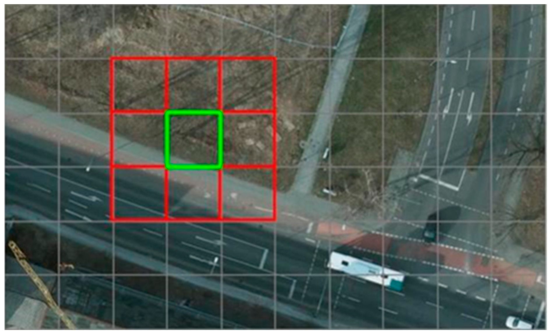
The superpixel generation module (spixel) aims to refine the dense classification branch and alleviate the blur of the object boundary. Initially, to generate superpixels, a common practice involves partitioning an H × W image into initial superpixel seeds using an h × w regular grid. Subsequently, each pixel p is assigned to one of these superpixel seeds g by finding a mapping Q. In practice, to simplify computational complexity, a pixel is typically assigned category labels within the neighborhood range of the seed points until no further changes occur in the clustering centers of each superpixel. For a given pixel p, neighboring grid cells within its own grid and the adjacent 8 grids are considered for assignment, as depicted in Figure 2. As outlined in previous literature [44], a soft association map Q can be formulated as: Q H × W × N p . Here, N p = 9 denotes the 9-neighborhood grid of a pixel. In this section, we utilize the last feature map produced by the top-down pathway of FPN to predict the soft association mapping Q. Specifically, the spixel module, composed of three 3 × 3 convolution layers, processes the aforementioned 512-depth feature map to a feature map Q with 9 channels, representing the probability that a given pixel belongs to its 9 neighborhood grids. Mathematically, q i , j n ( p ) denotes the likelihood that pixel p is allocated to the nth grid, with the constraint N q i , j n ( p ) = 1 . The closer q i , j n ( p ) is to 1, the higher the probability that pixel p belongs to the nth superpixel. During model training, the feature map Q generated by the superpixel module is iteratively updated. Consequently, the module produces the pixel–superpixel association map Q as its output.

3.3. Superpixel-Based Upsampling and Refinement

In the final stage of the proposed network, the soft association mapping Q was used to bridge pixel representation and superpixel representation, and then the semantic segmentation results at 1/4 scale were upsampled based on superpixels; the region of superpixels was exploited to refine the pixel-based semantic segmentation results. Specifically, given a pixel p whose coordinate in the image is (i,j), the center of the superpixel could be computed using the association map Q predicted by the superpixel generation module, where f sp and l sp are the feature vector and location vector of superpixel n, respectively, as follows:
f sp = p : n N p f i , j ( p ) · q i , j n ( p ) p : n N p q i , j n ( p ) ,
l sp = p : n N p l i , j ( p ) · q i , j n ( p ) p : n N p q i , j n ( p ) ,
where f i , j ( p ) is the feature vector of pixel (i,j), l i , j ( p ) is the 2-D coordinate of pixel (i,j), N p is the group of superpixels around pixel p, and p : n N p q i , j n ( p ) is the normalization constant.
Alternatively, one can reconstruct the vectors of pixel p:
f i , j ( p ) = n N p f sp · q i , j n ( p ) ,
l i , j ( p ) = n N p l sp · q i , j n ( p ) ,
where f i , j ( p ) and l i , j ( p ) are the reconstructed feature and location of the pixel p. In this study, the pixel semantic segmentation results through superpixel refining were regarded as the reconstructed feature of the pixel (Equation (3)). Meanwhile, the position reconstruction process reinstated the feature to its original resolution within the image (Equation (4)). In practice, the 1/4-scale fused feature map generates a 1/4-scale semantic segmentation probability map in the segmentation branch (Figure 1). According to Equations (3) and (4), we can use the Q map to reconstruct it into a full-scale semantic segmentation map. During reconstruction, based on a majority voting strategy, the most frequent classification category within a superpixel region is assigned to all pixels contained in that superpixel. Consequently, the prediction of the model was obtained.

3.4. Loss Function

During the training phase, the loss function L s s utilizes a blend of cross-entropy loss L c e and dice loss L d i c e for the semantic segmentation branch, which can be formulated as:
L c e = 1 N i = 1 N k = 1 K y i k log ( y ^ i k ) ,
L d i c e = 1 2 N i = 1 N k = 1 K y i k y ^ i k y i k + y ^ i k ,
L s s = L c e + L d i c e ,
where the number of samples is denoted by n, y ^ i k denotes the probability that the i-th prediction belongs to class k, y i k signifies the i-th ground truth.
For the superpixel generation branch, a region-based loss L s p is defined as:
L s p = P E ( f sp ,   f i , j ( p ) ) + m S l sp l i , j ( p ) ,
where E (·,·) is the cross-entropy function, S is the superpixel sampling size, and m is set to 0.03 by default.
Thus, the total loss is formulated as:
L = L s s + α × L s p ,
where α is set to 0.5 by default.

4. Experimental Settings

4.1. Datasets

Vaihingen: The Vaihingen dataset is a renowned dataset affiliated with the ISPRS Urban Semantic Labeling Project. Comprising 33 aerial orthophoto images of very high spatial resolution, each image is equipped with three multispectral bands and a normalized digital surface model (nDSM) featuring a ground sampling distance (GSD) of 9 cm. The images are annotated into six categories. Seventeen images are designated for testing based on prior studies [19,20], while the remaining images are allocated for training, excluding nDSM data from the experiments.
Potsdam: The Potsdam dataset is another part of the ISPRS Test Project on Urban Semantic Labeling. The dataset covers a larger area and has a higher GSD (5 cm) than the Vaihingen. The Potsdam dataset comprises 38 images sized at 6000 × 6000 and the corresponding labels of six categories. Referring to the previous [19,20], we utilized 24 three-channel images (R-G-B) as a train set, reserving the remaining 14 images for testing. Similar to Vaihingen, the nDSM data were not involved.
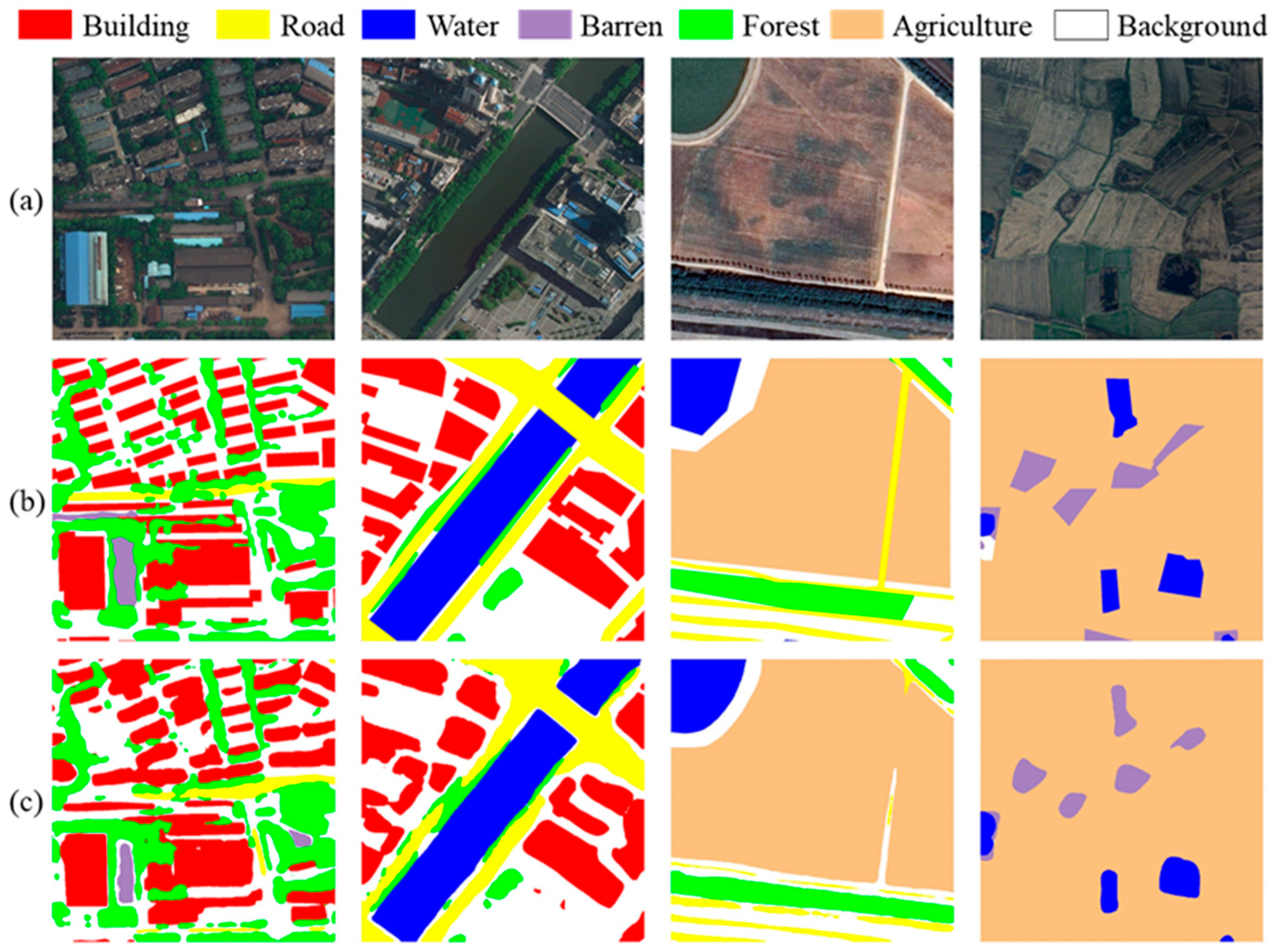
LoveDA (Wang et al. [53]): The LoveDA dataset comprises 5987 remote sensing images with a very high spatial resolution of 0.3 m, obtained from the Google Earth platform. Each 1024 × 1024 image is annotated with eight categories. The dataset is partitioned by the publisher into training (2522), validation (1669), and test sets (1796). Both the training and validation sets include images and corresponding pixel-level annotations, while the test set only provides images for prediction. Participants can upload the prediction results of the test set for online accuracy evaluation. The images in the dataset are sampled from urban and rural areas in three cities in China. Given the existence of multi-scale objects, intricate backgrounds, and regional disparities, this dataset poses substantial challenges for the models.
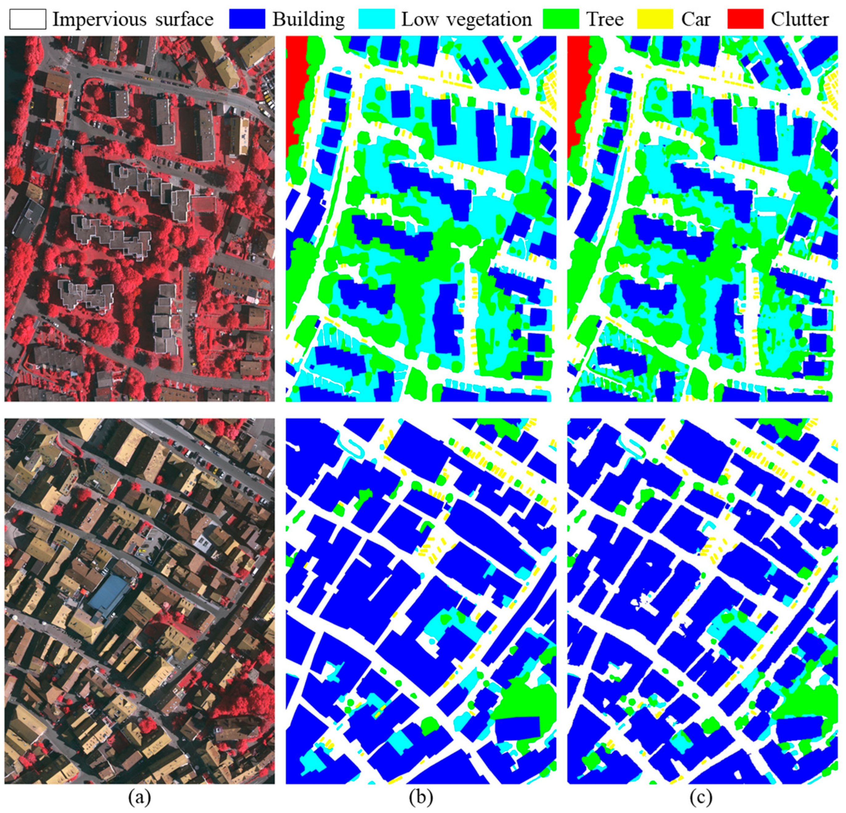
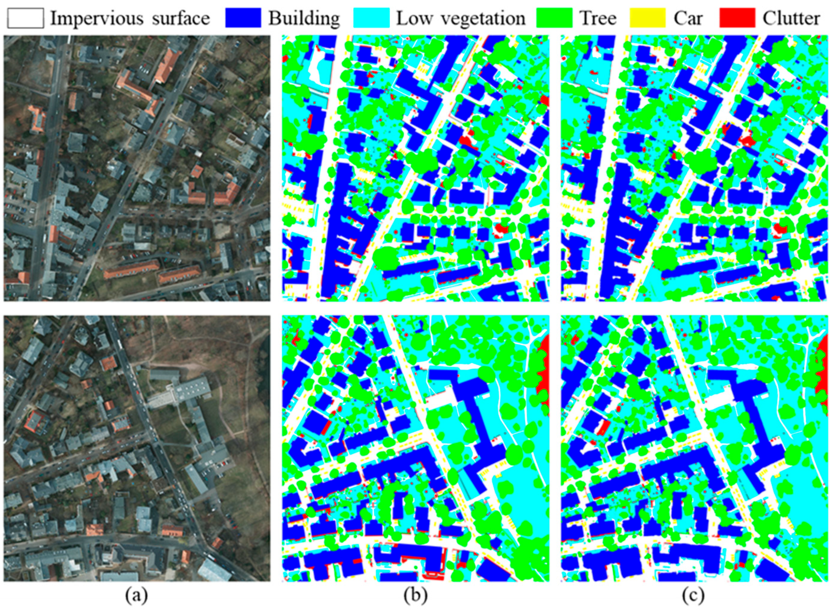
Figure 3 and Figure 4 show example images and labels of the above three datasets. These datasets, with their varying coverage, spatial resolutions, and complex objects, provide a comprehensive basis for evaluating the robustness and generalization of the developed model.

4.2. Implementation Details

Implemented using the PyTorch 1.13.1 package, the models in the experiments ran on an NVIDIA RTX 3090 GPU (24 GB). The Adma optimizer was employed, initialized with a learning rate of 1 × 10⁻⁴, using the cosine annealing strategy for fine-tuning. The grids with cell size 8 × 8 were used as the initial superpixels.
For the Vaihingen and Potsdam datasets, the original images were initially cropped into 1024 × 1024-pixel tiles using a sliding window approach with an overlap of 512 pixels. This was performed to ensure consistency with the tile size provided in the LoveDA dataset (i.e., 1024 × 1024 pixels). When training the model on each dataset, 512 × 512-pixel regions were randomly extracted from the 1024 × 1024-pixel tiles to be fed into the network, followed by data augmentation, including random rotations of 90 degrees, random vertical flips, and random horizontal flips; a batch size of four was used. The training epoch was set to 20 for the Potsdam and LoveDA datasets, while the number of training epochs for the Vaihingen dataset is 100 since the volume of the Vaihingen dataset is much smaller than the other two datasets. Additionally, an early stopping strategy on the validation set was applied to prevent overfitting. In the test phase, no test augmentation techniques were applied to the two ISPRS datasets, and only the multi-scale augmentation strategy ([0.5, 0.75, 1.0, 1.25, 1.5]) was applied to the LoveDA dataset.

4.3. Evaluation Metrics

The model performance was assessed using both the F1-score and the intersection over union (IoU). These two metrics of each category are calculated by:
F 1 = 2 × P r e c i s i o n × R e c a l l P r e c i s i o n + R e c a l l ,     P r e c i s i o n = T P T P + F P ,     R e c a l l = T P T P + F N ,
IoU = T P T P + F P + F N ,
where FP refers to false positive, FN to false negative, and TP to true positive. Furthermore, from all categories, the average of F1 (Avg. F1) and the average of IoU were also calculated.

4.4. Comparison Methods

We compared the proposed model with a series of advanced remote sensing semantic segmentation algorithms, including CNN-based methods, Transformer-based methods, and hybrids of transformer and CNN.
  • CNN-based networks: Deeplab v3plus [8], FuseNet [54].
  • Transformer-based networks: SwinUperNet [18], CG-Swin [19], STDSNet [55].
  • Hybrids of transformer and CNN: TransUNet [9], DC-Swin [56], UNetFormer [20].

5. Results and Analysis

5.1. Results Obtained from the ISPRS Datasets

Table 1 presents the numerical results acquired from the Vaihingen dataset. The proposed ESPNet demonstrated superior performance compared to other methods, achieving the highest mean F1 and mIoU scores across the test set. Notably, our method attained an impressive F1-score of 90.11% for the “Car” class, surpassing competing methods by at least 1.6%. Additionally, while the pure transformer method CG-Swin and the hybrid method TransUNet achieved leading F1-scores on the remaining classes, our method closely followed with a slight margin in F1-scores for these classes. Visualization of the predictions for IDs 2 and 4 can be observed in Figure 5.
Experiments were additionally conducted on the Potsdam dataset, which offers high spatial resolution and extensive coverage. Our proposed ESPNet achieved a mean F1-score of 93.54% and mIoU of 90.13% on the test set (Table 2). Notably, our ESPNet yielded outstanding performance across both overall accuracy measures, surpassing existing methods in four out of the five categories on the Potsdam.
The Vaihingen and Potsdam datasets are extensively employed for high-resolution image segmentation tasks. To date, a number of specially designed deep models have attained remarkable numerical accuracies on these two datasets. We showcase that our developed ESPNet achieves competitive scores compared with existing advanced networks. The visualization of results for ID 3_13 and 3_14 is presented in Figure 6.

5.2. Results Obtained from the LoveDA Dataset

To assess the performance of the proposed model, further experiments were carried out using the LoveDA dataset. It is noteworthy that the competition to provide this dataset is still open, and the results of the performance evaluation (only the IoU metric) are assessed and published by the organizer. Table 3 demonstrates the results of the LoveDA online test set. Our method achieved 55.73% of mIoU. The proposed method’s superiority is clear, as it surpasses other evaluated methods in both the IoU for individual categories and the overall mIoU. Examples of predictions are provided in Figure 7.

5.3. Ablation Experimental Results of Spixel Module

To explore the contribution of the introduced superpixel module, it is necessary to conduct the ablation experiment. For the ablation study, UperNet with ConvNeXt-T backbone was regarded as the baseline. As shown in Table 4, on different datasets, the employment of the superpixel generation module significantly enhanced the performance of the baseline model.
To further evaluate the flexibility of the spixel module, we further applied it to the existing CNN-based network and transformer-based network to conduct experiments. Specifically, Deeplab-v3plus and UperNet-Swin were chosen as benchmarks for the two types of networks mentioned above. According to the experimental findings presented in Table 5, the proposed superpixel module shows stable performance improvement when applied to networks with different architectures. For example, incorporating the superpixel module into Deeplab v3plus results in a 4.03% and 2.05% increase in mIoU on the ISPRS datasets, respectively. Due to the refining effect of learnable superpixels on object boundaries, the proposed superpixel generation module can effectively enhance the performance of existing segmentation networks.

5.4. Visualization Analysis

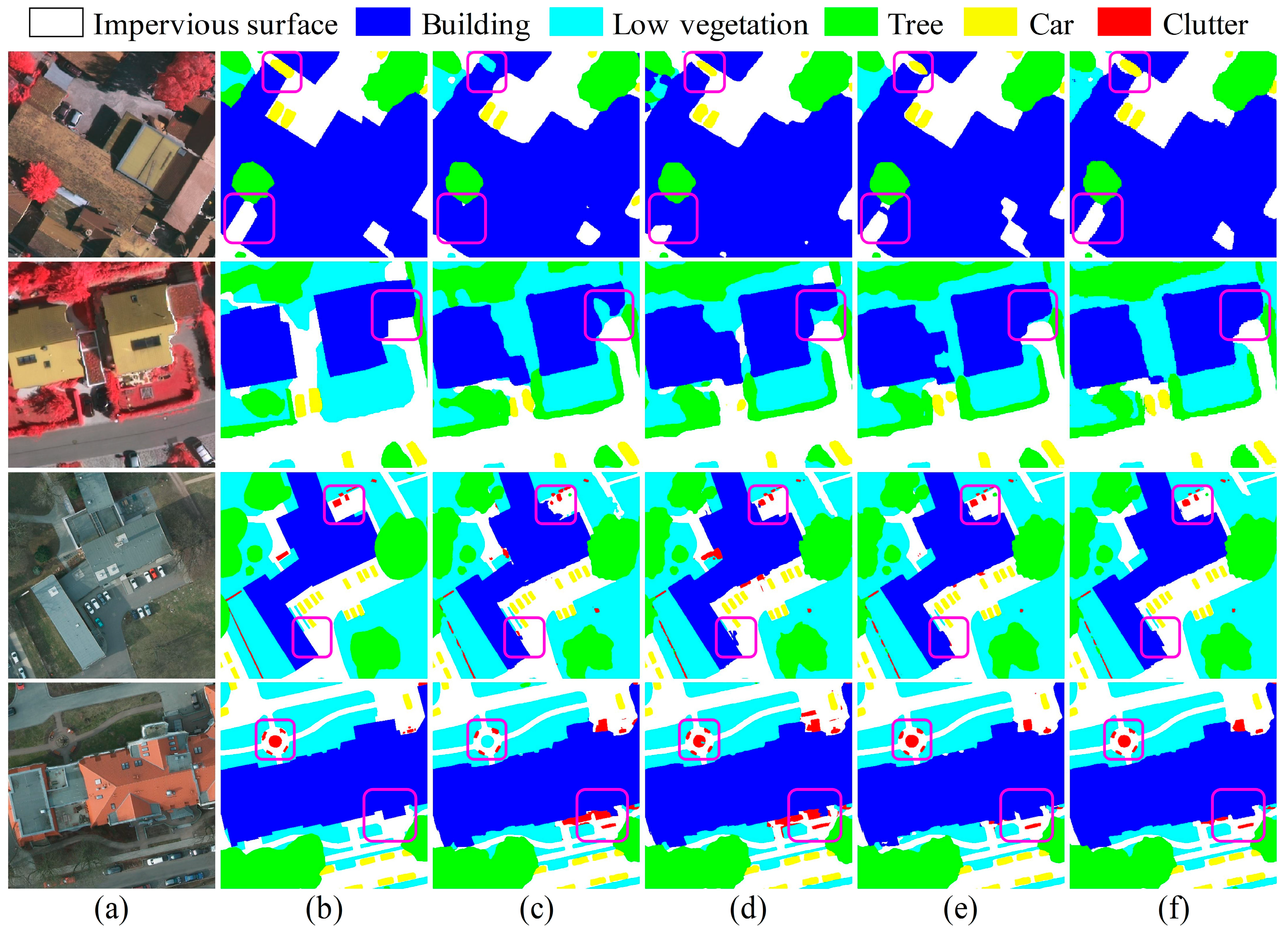
For a more thorough evaluation of the performance of the developed method in comparison to existing methods, Figure 8 presents enlarged visualizations for each method. The examples in the first and third rows illustrate the capability of our method in effectively identifying smaller target and object contours, whether it is the “Car” category, or shadows between buildings. The above observations are consistent with our expectations and show that the superpixel module can capture more precise edges, which is beneficial for preserving small-size objects. Further, the second row clearly demonstrates that some methods encounter difficulties in identifying the portion of the building obscured by vegetation due to the issue of semantic confusion. In comparison, ESPNet is still able to show more complete and accurate predictions. The results in the fourth row also demonstrate that the prediction generated by the developed method exhibits reduced noise and more accurate edges. Additionally, the edge visualizations show that the proposed method can capture finer edge details (Figure A1). This illustrates that the modified ConvNeXt network in this paper is adept at effectively extracting discriminative features.

5.5. Model Efficiency

The model performance is further compared on the Potsdam dataset using parameters and complexity, where the complexity metric FLOPs is measured using 512 × 512 × 3 inputs on a single NVIDIA RTX 3090 GPU. It is worth noting that the statistics for Deeplab v3plus, TransUNet, and SwinUPerNet were acquired through model reproduction, whereas data for the other comparison methods were extracted from their original reports. As shown in Table 6, the CNN-based method generally exhibits fewer parameters. However, when comparing model complexity to the Transformer-based model, there is no significant difference observed. Our ESPNet demonstrates comparable computational efficiency to Deeplab v3plus and SwinUperNet in terms of FLOPS and achieves superior accuracy. This outcome is attributed to the prioritization of accuracy over computational efficiency within our proposed method, emphasizing a balanced trade-off between the two. Therefore, we believe that the ESPNet model holds promising prospects in VHR remote sensing semantic segmentation.

5.6. Advantages of the Methodology

The proposed ESPNet, along with its constituent modules, underwent comprehensive evaluation across three VHR datasets. Evaluation results revealed that ESPNet achieves performance on par with state-of-the-art methods, owing to the combined strengths of its backbone network, the adaptable superpixel module, and the superpixel-enhanced upsampling strategy.
  • The convnext backbone network. ConvNext draws inspiration from the hierarchical design of vision transformers but is entirely constructed from standard convnet modules. The “sliding window” strategy of convnets is an intrinsic feature of visual processing. The basic blocks of ConvNext utilize large 7 × 7 convolutional kernels, enabling it to excel in handling high-resolution images. Leveraging ConvNext’s strong capability in extracting discriminative features, we propose the use of multi-scale fused FPN features for the mainline semantic segmentation. Additionally, we employ high-resolution feature maps from the final FPN layer for the superpixel generation branch. Experimental results confirm the effectiveness of the improved network proposed in this study.
  • The learnable superpixel module and the superpixel-enhanced upsampling strategy. As a re-representation of images, superpixels can complement object-level or sub-object-level shape prior information for pixel-wise segmentation. This is advantageous for improving object edge delineation in remote sensing semantic segmentation, although its effectiveness relies on the quality of superpixel generation. Similar to existing object-based CNN methods [26,37,38], the proposed method aims to exploit the object-level details. However, most methods are constrained by the non-differentiable algorithm of OBIA, separating deep segmentation from OBIA-based post-processing. In contrast, the learnable superpixel module introduced in this work can be embedded into the deep segmentation network, significantly accelerating the overall inference speed (Table A2). Furthermore, unlike the two-stage methods that extract features using CNNs for subsequent iterative superpixel generation [45], we explored directly generating learnable superpixels using a branch network to assist the main semantic segmentation task. As the parameters of the segmentation network are updated, the shape of the superpixels generated by the proposed module is iteratively optimized (Figure 9). By combining the two pathways through the superpixel-enhanced upsampling, the semantic segmentation and superpixel generation processes are incorporated into a complete one-stage FCN architecture. Additionally, the parameter size of the Spixel module is approximately 0.63 MB, and its computational complexity FLOPs is 10.28 G. This indicates that the module constitutes only a small fraction of the overall model’s size (as shown in Table 6), further underscoring its convenience. In this study, the introduction of the superpixel module enables the segmentation network to focus more on small objects during training. This leads to a significant improvement in accuracy for smaller objects, such as the “Car” category. Moreover, feature extraction, task-specific superpixel generation, and semantic segmentation stages are trained simultaneously under a unified end-to-end framework according to the task-specific loss functions. Thus, the output of semantic segmentation can be further refined.

5.7. Limitations and Future Work

In this study, the modified ConvNeXt backbone network not only enhances model accuracy but also leads to an increase in model complexity. Therefore, it is possible to further streamline the model architecture to better adapt to different types of remote sensing tasks. This study explored the use of the pixel–superpixel correlation matrix generated by the end-to-end superpixel branch as prior knowledge to help semantic segmentation, which inspired our subsequent work to integrate other prior knowledge of the remote sensing community into the deep network framework for further improvement. On the other hand, future experiments on a wider geographical area, more diverse land cover types, and across datasets can further verify the performance of the developed model in practical applications. Finally, it would be interesting to investigate the application of learnable superpixel modules to semi-supervised or unsupervised remote sensing classification.

6. Conclusions

This study presents ESPNet, an innovative CNN-based approach tailored for VHR image semantic segmentation. ESPNet leverages a differentiable superpixel generation method to assist in learning priors on object edges. Then, a superpixel-driven upsampling strategy is applied to retrieve edge information. The integration of the differentiable superpixel module and semantic segmentation within a cohesive framework facilitates training for optimal parameter acquisition. The proposed method achieved mIoU scores of 84.32, 90.13, and 55.73 on the Vaihingen, Pots-dam, and LoveDA datasets, respectively, demonstrating performance on par with state-of-the-art methods. Moreover, the developed superpixel module exhibits robustness and flexibility when applied across various deep network architectures.

Author Contributions

Conceptualization, Z.Y. and D.K.; methodology, Z.Y.; software, Z.Y. and B.D.; validation, B.D. and Y.L.; formal analysis, B.D.; investigation, Y.L.; resources, D.K.; data curation, M.D.; writing—original draft preparation, Z.Y.; writing—review and editing, Y.L. and X.T.; visualization, X.T.; supervision, D.K.; project administration, Y.L. and M.D.; funding acquisition, Z.Y. All authors have read and agreed to the published version of the manuscript.

Funding

This research was funded by the National Natural Science Foundation of China, grant number 42201300, and the Zhejiang Provincial Basic Public Welfare Research Project of China under grant number LGN22C130016.

Data Availability Statement

The datasets presented in this article are openly available in ISPRS at https://www.isprs.org/education/benchmarks/UrbanSemLab/Default.aspx (accessed on 2 July 2024) and LoveDA Semantic Segmentation Challenge at https://github.com/Junjue-Wang/LoveDA (accessed on 2 July 2024). The remaining data that support the findings in this study are available on request from the corresponding author.

Conflicts of Interest

The authors declare no conflicts of interest.

Appendix A

Our segmentation framework is adapted from UperNet, utilizing ConvNeXt-T as the backbone. As indicated in Table A1, the convnext-t-based FPN is competitive, and the additional accuracy gains brought by PPM illustrate its compatibility with FPN. Furthermore, empirically fusing the feature maps from the four stages in FPN is found to yield better performance. Lastly, the introduction of the superpixel module substantially improves the segmentation performance of the network.
Table A1. Ablation experiment of the proposed ESPNet on the Vaihingen dataset. The best value in each column is shown in bold.
MethodBackboneMean F1mIoU
FPNConvNeXt-T89.2482.18
FPN + PPMConvNeXt-T89.6182.27
UperNet (FPN + PPM + Fusion)ConvNeXt-T90.4583.55
ESPNet (FPN + PPM + Fusion + Spixel)ConvNeXt-T91.0684.32
Both our method and the object-based CNN method introduce information about the object to strengthen the edge information of the object. Under the premise of using the same segmentation network, the difference is that the object-based CNN method introduces the graph-based object segmentation (Graph-Seg) in the post-processing stage, which is separate from the CNN network. The proposed method integrates the superpixel generation module into the deep segmentation network to become an end-to-end deep framework. As shown in Table A2, compared with the previous object-CNN method, the proposed method has improved the accuracy and made a substantial breakthrough in inference speed. This is mainly because processes such as differentiable superpixel generation and superpixel-enhanced upsampling can take advantage of the GPU’s high-speed computing power.
Table A2. Comparison with OBIA-driven CNNs on the Vaihingen test set.
MethodBackboneMean F1mIoUPrediction Time on Test Set
Object-based CNN [8]
(FPN + PPM + Fusion + Graph-Seg)
ConvNeXt-T90.7683.794099 min 30 s
ESPNet (FPN + PPM + Fusion + Spixel)ConvNeXt-T91.06 84.321 min 35 s
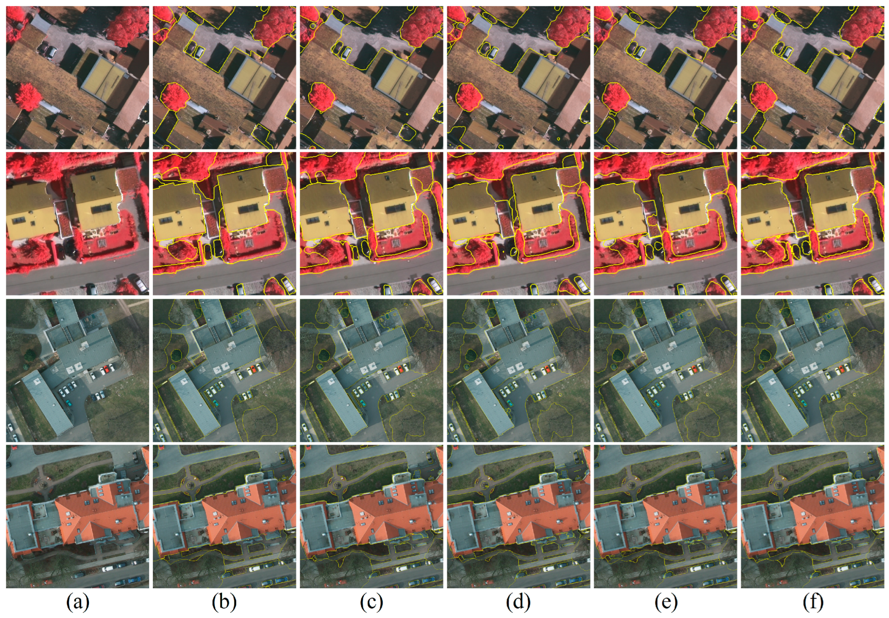
Figure A1. Visualization of edges on the ISPRS test sets. (a) Images, (b) Ground Truth, (c) Deeplab v3plus, (d) SwinUperNet, (e) Upernet-ConvNeXt, (f) the proposed ESPNet. The yellow lines indicate the boundaries of the segmented objects.
Remotesensing 16 03805 g0a1

References

  1. Long, J.; Shelhamer, E.; Darrell, T. Fully Convolutional Networks for Semantic Segmentation. In Proceedings of the CVPR, Boston, MA, USA, 7–12 June 2015; pp. 3431–3440. [Google Scholar]
  2. Ma, L.; Liu, Y.; Zhang, X.; Ye, Y.; Yin, G.; Johnson, B.A. Deep Learning in Remote Sensing Applications: A Meta-Analysis and Review. ISPRS J. Photogramm. Remote Sens. 2019, 152, 166–177. [Google Scholar] [CrossRef]
  3. Reichstein, M.; Camps-Valls, G.; Stevens, B.; Jung, M.; Denzler, J.; Carvalhais, N. Prabhat Deep Learning and Process Understanding for Data-Driven Earth System Science. Nature 2019, 566, 195–204. [Google Scholar] [CrossRef] [PubMed]
  4. Zhang, B.; Wu, Y.; Zhao, B.; Chanussot, J.; Hong, D.; Yao, J.; Gao, L. Progress and Challenges in Intelligent Remote Sensing Satellite Systems. IEEE J. Sel. Top. Appl. Earth Obs. Remote Sens. 2022, 15, 1814–1822. [Google Scholar] [CrossRef]
  5. Zhu, Q.; Zhang, Y.; Li, Z.; Yan, X.; Guan, Q.; Zhong, Y.; Zhang, L.; Li, D. Oil Spill Contextual and Boundary-Supervised Detection Network Based on Marine SAR Images. IEEE Trans. Geosci. Remote Sens. 2022, 60, 5213910. [Google Scholar] [CrossRef]
  6. Persello, C.; Grift, J.; Fan, X.; Paris, C.; Hänsch, R.; Koeva, M.; Nelson, A. AI4SmallFarms: A Dataset for Crop Field Delineation in Southeast Asian Smallholder Farms. IEEE Geosci. Remote Sens. Lett. 2023, 20, 2505705. [Google Scholar] [CrossRef]
  7. Ronneberger, O.; Fischer, P.; Brox, T. U-Net: Convolutional Networks for Biomedical Image Segmentation. In Proceedings of the MICCAI; Navab, N., Hornegger, J., Wells, W.M., Frangi, A.F., Eds.; Springer International Publishing: Berlin/Heidelberg, Germany, 2015; pp. 234–241. [Google Scholar]
  8. Chen, L.-C.; Zhu, Y.; Papandreou, G.; Schroff, F.; Adam, H. Encoder-Decoder with Atrous Separable Convolution for Semantic Image Segmentation. In Proceedings of the European Conference on Computer Vision (ECCV), Munich, Germany, 8–14 September 2018; pp. 801–818. [Google Scholar]
  9. Chen, J.; Lu, Y.; Yu, Q.; Luo, X.; Adeli, E.; Wang, Y.; Lu, L.; Yuille, A.L.; Zhou, Y. TransUNet: Transformers Make Strong Encoders for Medical Image Segmentation. arXiv 2021, arXiv:2102.04306. [Google Scholar]
  10. Li, R.; Zheng, S.; Zhang, C.; Duan, C.; Wang, L.; Atkinson, P.M. ABCNet: Attentive Bilateral Contextual Network for Efficient Semantic Segmentation of Fine-Resolution Remotely Sensed Imagery. ISPRS J. Photogramm. Remote Sens. 2021, 181, 84–98. [Google Scholar] [CrossRef]
  11. Yang, M.Y.; Kumaar, S.; Lyu, Y.; Nex, F. Real-Time Semantic Segmentation with Context Aggregation Network. ISPRS J. Photogramm. Remote Sens. 2021, 178, 124–134. [Google Scholar] [CrossRef]
  12. Mou, L.; Zhu, X.X. Learning to Pay Attention on Spectral Domain: A Spectral Attention Module-Based Convolutional Network for Hyperspectral Image Classification. IEEE Trans. Geosci. Remote Sens. 2019, 58, 110–122. [Google Scholar] [CrossRef]
  13. Shakeel, A.; Sultani, W.; Ali, M. Deep Built-Structure Counting in Satellite Imagery Using Attention Based Re-Weighting. ISPRS J. Photogramm. Remote Sens. 2019, 151, 313–321. [Google Scholar] [CrossRef]
  14. Zhao, W.; Du, S. Learning Multiscale and Deep Representations for Classifying Remotely Sensed Imagery. ISPRS J. Photogramm. Remote Sens. 2016, 113, 155–165. [Google Scholar] [CrossRef]
  15. Li, L. Deep Residual Autoencoder with Multiscaling for Semantic Segmentation of Land-Use Images. Remote Sens. 2019, 11, 2142. [Google Scholar] [CrossRef]
  16. Wang, J.; Zheng, Y.; Wang, M.; Shen, Q.; Huang, J. Object-Scale Adaptive Convolutional Neural Networks for High-Spatial Resolution Remote Sensing Image Classification. IEEE J. Sel. Top. Appl. Earth Obs. Remote Sens. 2021, 14, 283–299. [Google Scholar] [CrossRef]
  17. He, X.; Zhou, Y.; Zhao, J.; Zhang, D.; Yao, R.; Xue, Y. Swin Transformer Embedding UNet for Remote Sensing Image Semantic Segmentation. IEEE Trans. Geosci. Remote Sens. 2022, 60, 4408715. [Google Scholar] [CrossRef]
  18. Liu, Z.; Lin, Y.; Cao, Y.; Hu, H.; Wei, Y.; Zhang, Z.; Lin, S.; Guo, B. Swin Transformer: Hierarchical Vision Transformer Using Shifted Windows. In Proceedings of the ICCV, Montreal, QC, Canada, 11–17 October 2021; pp. 9992–10002. [Google Scholar]
  19. Meng, X.; Yang, Y.; Wang, L.; Wang, T.; Li, R.; Zhang, C. Class-Guided Swin Transformer for Semantic Segmentation of Remote Sensing Imagery. IEEE Geosci. Remote Sens. Lett. 2022, 19, 6517505. [Google Scholar] [CrossRef]
  20. Wang, L.; Li, R.; Zhang, C.; Fang, S.; Duan, C.; Meng, X.; Atkinson, P.M. UNetFormer: A UNet-like Transformer for Efficient Semantic Segmentation of Remote Sensing Urban Scene Imagery. ISPRS J. Photogramm. Remote Sens. 2022, 190, 196–214. [Google Scholar] [CrossRef]
  21. Blaschke, T.; Lang, S.; Hay, G.J. (Eds.) Object-Based Image Analysis: Spatial Concepts for Knowledge-Driven Remote Sensing Applications; Lecture Notes in Geoinformation and Cartography; Springer: Berlin/Heidelberg, Germany, 2008; ISBN 978-3-540-77057-2. [Google Scholar]
  22. Blaschke, T. Object Based Image Analysis for Remote Sensing. ISPRS J. Photogramm. Remote Sens. 2010, 65, 2–16. [Google Scholar] [CrossRef]
  23. Huang, X.; Lu, Q.; Zhang, L. A Multi-Index Learning Approach for Classification of High-Resolution Remotely Sensed Images over Urban Areas. ISPRS J. Photogramm. Remote Sens. 2014, 90, 36–48. [Google Scholar] [CrossRef]
  24. Geiss, C.; Klotz, M.; Schmitt, A.; Taubenbock, H. Object-Based Morphological Profiles for Classification of Remote Sensing Imagery. IEEE Trans. Geosci. Remote Sens. 2016, 54, 5952–5963. [Google Scholar] [CrossRef]
  25. Liu, T.; Gu, Y.; Chanussot, J.; Dalla Mura, M. Multimorphological Superpixel Model for Hyperspectral Image Classification. IEEE Trans. Geosci. Remote Sens. 2017, 55, 6950–6963. [Google Scholar] [CrossRef]
  26. Zhao, W.; Du, S.; Emery, W.J. Object-Based Convolutional Neural Network for High-Resolution Imagery Classification. IEEE J. Sel. Top. Appl. Earth Obs. Remote Sens. 2017, 10, 3386–3396. [Google Scholar] [CrossRef]
  27. Liang, L.; Meyarian, A.; Yuan, X.; Runkle, B.R.K.; Mihaila, G.; Qin, Y.; Daniels, J.; Reba, M.L.; Rigby, J.R. The First Fine-Resolution Mapping of Contour-Levee Irrigation Using Deep Bi-Stream Convolutional Neural Networks. Int. J. Appl. Earth Obs. Geoinf. 2021, 105, 102631. [Google Scholar] [CrossRef]
  28. Liu, Z.; Mao, H.; Wu, C.-Y.; Feichtenhofer, C.; Darrell, T.; Xie, S. A ConvNet for the 2020s. In Proceedings of the CVPR, New Orleans, LA, USA, 18–24 June 2022; pp. 11966–11976. [Google Scholar]
  29. Maggiori, E.; Tarabalka, Y.; Charpiat, G.; Alliez, P. High-Resolution Aerial Image Labeling With Convolutional Neural Networks. IEEE Trans. Geosci. Remote Sens. 2017, 55, 7092–7103. [Google Scholar] [CrossRef]
  30. Ye, Z.; Fu, Y.; Gan, M.; Deng, J.; Comber, A.; Wang, K. Building Extraction from Very High Resolution Aerial Imagery Using Joint Attention Deep Neural Network. Remote Sens. 2019, 11, 2970. [Google Scholar] [CrossRef]
  31. Ding, L.; Tang, H.; Bruzzone, L. LANet: Local Attention Embedding to Improve the Semantic Segmentation of Remote Sensing Images. IEEE Trans. Geosci. Remote Sens. 2021, 59, 426–435. [Google Scholar] [CrossRef]
  32. Zhang, Y.; Liu, H.; Hu, Q. Transfuse: Fusing Transformers and Cnns for Medical Image Segmentation. In Proceedings of the Medical Image Computing and Computer Assisted Intervention–MICCAI 2021: 24th International Conference, Proceedings, Part I 24. Strasbourg, France, 27 September–1 October 2021; Springer: Berlin/Heidelberg, Germany, 2021; pp. 14–24. [Google Scholar]
  33. Vaswani, A.; Shazeer, N.; Parmar, N.; Uszkoreit, J.; Jones, L.; Gomez, A.N.; Kaiser, Ł.; Polosukhin, I. Attention Is All You Need. Adv. Neural Inf. Process. Syst. 2017, 30, 6000–6010. [Google Scholar]
  34. Fu, Y.; Liu, K.; Shen, Z.; Deng, J.; Gan, M.; Liu, X.; Lu, D.; Wang, K. Mapping Impervious Surfaces in Town–Rural Transition Belts Using China’s GF-2 Imagery and Object-Based Deep CNNs. Remote Sens. 2019, 11, 280. [Google Scholar] [CrossRef]
  35. Zhang, C.; Yue, P.; Tapete, D.; Shangguan, B.; Wang, M.; Wu, Z. A Multi-Level Context-Guided Classification Method with Object-Based Convolutional Neural Network for Land Cover Classification Using Very High Resolution Remote Sensing Images. Int. J. Appl. Earth Obs. Geoinf. 2020, 88, 102086. [Google Scholar] [CrossRef]
  36. Huang, B.; Zhao, B.; Song, Y. Urban Land-Use Mapping Using a Deep Convolutional Neural Network with High Spatial Resolution Multispectral Remote Sensing Imagery. Remote Sens. Environ. 2018, 214, 73–86. [Google Scholar] [CrossRef]
  37. Zhang, C.; Sargent, I.; Pan, X.; Li, H.; Gardiner, A.; Hare, J.; Atkinson, P.M. An Object-Based Convolutional Neural Network (OCNN) for Urban Land Use Classification. Remote Sens. Environ. 2018, 216, 57–70. [Google Scholar] [CrossRef]
  38. Ma, Y.; Deng, X.; Wei, J. Land Use Classification of High-Resolution Multispectral Satellite Images with Fine-Grained Multiscale Networks and Superpixel Post Processing. IEEE J. Sel. Top. Appl. Earth Obs. Remote Sens. 2023, 16, 3264–3278. [Google Scholar] [CrossRef]
  39. Dong, D.; Ming, D.; Weng, Q.; Yang, Y.; Fang, K.; Xu, L.; Du, T.; Zhang, Y.; Liu, R. Building Extraction from High Spatial Resolution Remote Sensing Images of Complex Scenes by Combining Region-Line Feature Fusion and OCNN. IEEE J. Sel. Top. Appl. Earth Obs. Remote Sens. 2023, 16, 4423–4438. [Google Scholar] [CrossRef]
  40. Nixon, M.S.; Aguado, A.S. 8—Region-Based Analysis. In Feature Extraction and Image Processing for Computer Vision, 4th ed.; Nixon, M.S., Aguado, A.S., Eds.; Academic Press: Cambridge, MA, USA, 2020; pp. 399–432. ISBN 978-0-12-814976-8. [Google Scholar]
  41. Blaschke, T.; Hay, G.J.; Kelly, M.; Lang, S.; Hofmann, P.; Addink, E.; Queiroz Feitosa, R.; van der Meer, F.; van der Werff, H.; van Coillie, F.; et al. Geographic Object-Based Image Analysis—Towards a New Paradigm. ISPRS J. Photogramm. Remote Sens. 2014, 87, 180–191. [Google Scholar] [CrossRef] [PubMed]
  42. Zanotta, D.C.; Zortea, M.; Ferreira, M.P. A Supervised Approach for Simultaneous Segmentation and Classification of Remote Sensing Images. ISPRS J. Photogramm. Remote Sens. 2018, 142, 162–173. [Google Scholar] [CrossRef]
  43. Jampani, V.; Sun, D.; Liu, M.-Y.; Yang, M.-H.; Kautz, J. Superpixel Sampling Networks. arXiv 2018, arXiv:1807.10174. [Google Scholar]
  44. Yang, F.; Sun, Q.; Jin, H.; Zhou, Z. Superpixel Segmentation with Fully Convolutional Networks. In Proceedings of the CVPR, Seattle, WA, USA, 16–18 June 2020; pp. 13961–13970. [Google Scholar]
  45. Mi, L.; Chen, Z. Superpixel-Enhanced Deep Neural Forest for Remote Sensing Image Semantic Segmentation. ISPRS J. Photogramm. Remote Sens. 2020, 159, 140–152. [Google Scholar] [CrossRef]
  46. Zhang, H.; Zou, J.; Zhang, L. EMS-GCN: An End-to-End Mixhop Superpixel-Based Graph Convolutional Network for Hyperspectral Image Classification. IEEE Trans. Geosci. Remote Sens. 2022, 60, 5526116. [Google Scholar] [CrossRef]
  47. Ma, F.; Zhang, F.; Xiang, D.; Yin, Q.; Zhou, Y. Fast Task-Specific Region Merging for SAR Image Segmentation. IEEE Trans. Geosci. Remote Sens. 2022, 60, 5222316. [Google Scholar] [CrossRef]
  48. Yu, H.; Hu, H.; Xu, B.; Shang, Q.; Wang, Z.; Zhu, Q. SuperpixelGraph: Semi-Automatic Generation of Building Footprint through Semantic-Sensitive Superpixel and Neural Graph Networks. Int. J. Appl. Earth Obs. Geoinf. 2023, 125, 103556. [Google Scholar] [CrossRef]
  49. Xiao, T.; Liu, Y.; Zhou, B.; Jiang, Y.; Sun, J. Unified Perceptual Parsing for Scene Understanding. In Proceedings of the ECCV, Computer Vision, Munich, Germany, 8–14 September 2018; Ferrari, V., Hebert, M., Sminchisescu, C., Weiss, Y., Eds.; Volume 11209, pp. 432–448. [Google Scholar]
  50. Zhao, H.; Shi, J.; Qi, X.; Wang, X.; Jia, J. Pyramid Scene Parsing Network. In Proceedings of the CVPR, Honolulu, HI, USA, 21–26 July 2017; pp. 6230–6239. [Google Scholar]
  51. Lin, T.-Y.; Dollár, P.; Girshick, R.; He, K.; Hariharan, B.; Belongie, S. Feature Pyramid Networks for Object Detection. In Proceedings of the CVPR, Honolulu, HI, USA, 21–26 July 2017; pp. 936–944. [Google Scholar]
  52. Liu, W.; Liu, J.; Luo, Z.; Zhang, H.; Gao, K.; Li, J. Weakly Supervised High Spatial Resolution Land Cover Mapping Based on Self-Training with Weighted Pseudo-Labels. Int. J. Appl. Earth Obs. Geoinf. 2022, 112, 102931. [Google Scholar] [CrossRef]
  53. Wang, J.; Zheng, Z.; Ma, A.; Lu, X.; Zhong, Y. LoveDA: A Remote Sensing Land-Cover Dataset for Domain Adaptive Semantic Segmentation. In Proceedings of the Neural Information Processing Systems Track on Datasets and Benchmarks; Vanschoren, J., Yeung, S., Eds.; Curran Associates, Inc.: Red Hook, NY, USA, 2021; Volume 1. [Google Scholar]
  54. Audebert, N.; Le Saux, B.; Lefèvre, S. Beyond RGB: Very High Resolution Urban Remote Sensing with Multimodal Deep Networks. ISPRS J. Photogramm. Remote Sens. 2018, 140, 20–32. [Google Scholar] [CrossRef]
  55. Zhou, X.; Zhou, L.; Gong, S.; Zhong, S.; Yan, W.; Huang, Y. Swin Transformer Embedding Dual-Stream for Semantic Segmentation of Remote Sensing Imagery. IEEE J. Sel. Top. Appl. Earth Obs. Remote Sens. 2024, 17, 175–189. [Google Scholar] [CrossRef]
  56. Wang, L.; Li, R.; Duan, C.; Zhang, C.; Meng, X.; Fang, S. A Novel Transformer Based Semantic Segmentation Scheme for Fine-Resolution Remote Sensing Images. IEEE Geosci. Remote Sens. Lett. 2022, 19, 6506105. [Google Scholar] [CrossRef]
Figure 1. The framework of ESPNet.
Remotesensing 16 03805 g001
Figure 2. Diagram of Np. Within the green box, solely the adjacent nine grids within the red box are selected for allocation to each pixel.
Remotesensing 16 03805 g002
Figure 3. Examples from Vaihingen and Potsdam datasets. (a) An example image of Vaihingen, (b) Ground Truth, (c) an example image of Potsdam, (d) Ground Truth.
Remotesensing 16 03805 g003
Figure 4. Examples from LoveDA dataset. (a) An example image of an urban area, (b) Ground Truth, (c) an example image of a rural area, (d) Ground Truth.
Remotesensing 16 03805 g004
Figure 5. Predicted results of ID 2 (top) and 4 (bottom) on the Vaihingen. (a) Images, (b) Ground Truth, (c) the proposed ESPNet.
Remotesensing 16 03805 g005
Figure 6. Predicted results of ID 3_13 (top) and 3_14 (bottom) on the Potsdam. (a) Images, (b) Ground Truth, (c) the proposed ESPNet.
Remotesensing 16 03805 g006
Figure 7. Examples of predicted results on the LoveDA validation set. (a) Images, (b) Ground Truth, (c) the proposed ESPNet.
Remotesensing 16 03805 g007
Figure 8. Visualization comparisons on the ISPRS test sets. (a) Images, (b) Ground Truth, (c) Deeplab v3plus, (d) SwinUperNet, (e) Upernet-ConvNeXt, (f) the proposed ESPNet. The purple boxes are added to highlight the differences.
Remotesensing 16 03805 g008
Figure 9. The example of superpixel generation. (a) Images, (b) Superpixel grids at the beginning of training, (c) Superpixels generated near the end of training, (d) Semantic Segmentation after superpixel-enhanced upsampling.
Remotesensing 16 03805 g009
Table 1. Quantitative evaluation on the test set of Vaihingen. The best value in each column is shown in bold.
MethodBackboneF1-ScoreMean F1mIoU
Imp. Surf.BuildingLow Veg.TreeCar
Deeplab v3plus [8]ResNet10190.8993.2582.1288.6780.6387.1178.73
V-FuseNet [54]VGG-1691.0094.4084.5089.9086.3089.20
TransUNet [9]VIT-Res5091.6696.4876.1492.7769.5687.3478.26
CG-Swin [19]Swin-S93.5596.2485.7090.5987.9890.8183.39
UNetFormer [20]ResNet1892.7095.3084.9090.6088.5090.4082.70
STDSNet [55]Swin-B86.0992.1872.8281.1776.5789.8181.77
ESPNet (Ours)ConvNeXt-T93.4396.2385.3690.1790.1191.0684.32
Table 2. Quantitative evaluation on the test set of Potsdam. The best value in each column is shown in bold.
MethodBackboneF1-ScoreMean F1mIoU
Imp. Surf.BuildingLow Veg.TreeCar
Deeplab v3plus [8]ResNet10192.0796.1986.3987.9494.6691.4587.22
V-FuseNet [54]VGG-1692.7096.3087.3088.5095.4092.04
TransUNet [9]VIT-Res5091.9396.6389.9882.6593.1790.9783.74
CG-Swin [19]Swin-S94.0797.4288.5389.7496.6193.2887.61
UNetFormer [20]ResNet1893.6097.2087.7088.9096.5092.8086.80
STDSNet [55]Swin-B84.9092.2374.0976.2284.2190.1782.33
ESPNet (Ours)ConvNeXt-T94.3897.6388.7790.1196.8093.5490.13
Table 3. Quantitative evaluation on the test set of LoveDA. The best value in each column is shown in bold.
MethodBackboneIoUmIoU
BackgroundBuildingRoadWaterBarrenForestAgriculture
Deeplab v3plus [8]ResNet10143.7554.6151.6078.7520.8242.6265.7851.13
TransUNet [9]VIT-Res5043.0056.1053.7078.09.3044.9056.9048.90
SwinUperNet [18]Swin-T43.3054.3054.3078.7014.9045.3059.6050.00
DC-Swin [56]Swin-T41.3054.5056.2078.1014.5047.2062.4050.60
UNetFormer [20]ResNet1844.7058.8054.9079.6020.1046.0062.5052.40
ESPNet (Ours)ConvNeXt-T49.4362.0259.1182.3617.9350.0269.2755.73
Table 4. Ablation experiment of spixel module on the three datasets. The best value in each column is shown in bold.
DatasetMethodBackboneMean F1mIoU
VaihingenUperNetConvNeXt-T 90.4583.55
ESPNetConvNeXt-T91.0684.32
PotsdamUperNetConvNeXt-T 93.0689.59
ESPNetConvNeXt-T93.5490.13
LoveDAUperNetConvNeXt-T 54.75
ESPNetConvNeXt-T55.73
Table 5. Ablation experiment of spixel module on the deep networks.
DatasetMethodBackboneMean F1mIoU
VaihingenDeeplab v3plusResNet10187.1178.73
Deeplab v3plus + spixelResNet10189.6982.76
UperNetSwin-B89.6182.27
UperNet + spixelSwin-B90.1082.98
PotsdamDeeplab v3plusResNet10191.4587.22
Deeplab v3plus + spixelResNet10192.9689.27
UperNetSwin-B92.6488.92
UperNet + spixelSwin-B93.3290.05
LoveDADeeplab v3plusResNet10151.13
Deeplab v3plus + spixelResNet10152.23
UperNetSwin-B52.84
UperNet + spixelSwin-B53.64
Table 6. Comparison of model parameters and complexity.
MethodBackboneParameters/MBFLOPs/GmIoU
Deeplab v3plus [8]ResNet10160.21254.8987.22
TransUNet [9]VIT-Res50100.44129.4483.74
SwinUperNet [18]Swin-B64.01247.3888.92
UNetFormer [20]ResNet1811.6811.7486.80
CG-Swin [19]Swin-S50.35/87.61
STDSNet [55]Swin-B130.13327.6682.33
ESPNet (Ours)ConvNeXt-T82.50253.4590.13
Disclaimer/Publisher’s Note: The statements, opinions and data contained in all publications are solely those of the individual author(s) and contributor(s) and not of MDPI and/or the editor(s). MDPI and/or the editor(s) disclaim responsibility for any injury to people or property resulting from any ideas, methods, instructions or products referred to in the content.