Article

Simulating High-Resolution Sun-Induced Chlorophyll Fluorescence Image of Three-Dimensional Canopy Based on Photon Mapping

State Key Laboratory of Remote Sensing Science, Faculty of Geographical Science, Beijing Normal University, Beijing 100875, China
*
Author to whom correspondence should be addressed.
Remote Sens. 2024, 16(20), 3783; https://doi.org/10.3390/rs16203783
Submission received: 23 September 2024 / Accepted: 8 October 2024 / Published: 11 October 2024

Abstract

:
The remote sensing of sun-induced chlorophyll fluorescence (SIF) is an emerging technique with immense potential for terrestrial vegetation sciences. However, the interpretation of fluorescence data is often hindered by the complexity of observed land surfaces. Therefore, advanced remote sensing models, particularly physically based simulations, are critical to accurately interpret SIF data. In this work, we propose a three-dimensional (3D) radiative transfer model that employs the Monte Carlo ray-tracing technique to simulate the excitation and transport of SIF within plant canopies. This physically based approach can quantify the various radiative processes contributing to the observed SIF signal with high fidelity. The model’s performance is rigorously evaluated by comparing the simulated SIF spectra and angular distributions to field measurements, as well as conducting systematic comparisons with an established radiative transfer model. The results demonstrate the proposed model’s ability to reliably reproduce the key spectral and angular characteristics of SIF, with the coefficient of determination ( R 2 ) exceeding 0.98 and root mean square error (RMSE) being less than 0.08 mW m−2 sr−1 nm−1 for both the red and far-red fluorescence peaks. Furthermore, the model’s versatile representation of canopy structures, enabled by the decoupling of radiation and geometry, is applied to study the impact of 3D structure on SIF patterns. This capability makes the proposed model a highly attractive tool for investigating SIF distributions in realistic, heterogeneous canopy environments.

1. Introduction

Fluorescence refers to the process where an object absorbs light of a short wavelength and emits light of a longer wavelength, typically within approximately 10 8 seconds [1]. Chlorophyll fluorescence is an inherent signal given off by plants, which can be utilized to assess their physiological condition [2]. Fluorescence imaging is thus becoming one of the non-invasive and non-destructive methods with great potential that allow the long-term monitoring of plant activities [3]. Spectroscopy, particularly imaging spectroscopy, is commonly utilized to evaluate plant traits related to biochemistry, structure, and function, along with their dynamics [4,5]. The growing accessibility of high-resolution spectroradiometers now makes it feasible to measure SIF [6].
In remote sensing, passive measurements of sun-induced chlorophyll fluorescence (SIF) open up new opportunities for global vegetation monitoring such as improving the estimation of vegetation photosynthetic capacity and inferring the surface carbon fluxes [7,8,9].
The reported measurements from spaceborne sensors, such as GOME-2 [10], GOSAT [11], OCO-2 [12], TROPOMI [13], and TanSat [14], provide quantitative mapping of SIF satellite data, revealing the potential to enhance the understanding of terrestrial vegetation gross primary production and further the global carbon cycle [15]. And the FLEX mission by the European Space Agency (ESA) has been specifically designed and optimized to map SIF [16]. Moreover, SIF measurements from airborne [17], and ground [18,19,20] sensors have demonstrated the capability to successfully retrieve this signal at the top of the canopy. The combination of spaceborne, airborne, and ground measurements reveals novel understandings of the spatial distribution of vegetation fluorescence, ranging from individual leaves to the ecosystem scale.
SIF is also viewed as a new technique in the field of phenotyping. Recent advancements in SIF retrieval enable sophisticated high-throughput phenotyping systems to efficiently detect subtle early stress at the canopy level [21]. It has the advantage of being applied to large fields, aircraft surveys, and satellites [22].
However, scaling fluorescence from leaf to canopy remains a great challenge [23]. The heterogeneity of the vegetation canopy usually complicates the interpretation of canopy SIF observations. Multiple scattering of SIF in the canopy by leaves and stems causes the reabsorption of the red SIF [15]. Furthermore, sunlit leaves generally generate higher SIF because they receive more intense light compared to shaded leaves that are illuminated by weaker, diffuse light [18]. Additionally, it is important to consider that photosynthetic active radiation (PAR) levels influence fluorescence correction factors. This dependency contributes to the spatial heterogeneity of SIF emittance across different parts of the canopy (Appendix A). Therefore, remote sensing models, particularly physically based models, that simulate the observations are critical to correctly interpret the fluorescence data.
While direct field measurements are expensive and challenging, model simulation can help quantify the effects of methodological uncertainties (e.g., different viewing directions) on SIF retrieval by generating simulated remote sensing data and images. Simulation can control the noises and uncertain factors; in contrast, even slight measurement errors may cause significant biases in the retrieved SIF due to the weak signals. Modeling tests are also necessary prior to field campaigns to assess the potential of retrieval algorithms. More importantly and with great potential, models can form the foundation for additional research to evaluate the distribution of photosynthetic activity within plant canopies and help create methods to enhance crop photosynthesis.
Over the past years, various radiative transfer (RT) models, either the simple turbid medium approaches (one-dimensional (1D) models) or realistic vegetation models (three-dimensional (3D) models), have been developed to assess how leaf and canopy structures and geometries influence radiative fluxes across different wavelengths [24,25,26,27]. One-dimensional models are usually efficient due to their simplicity. The 1D model simulation could be accurate for the horizontally homogeneous scenarios as well, whereas the more complex 3D models are needed to simulate SIF over a heterogeneous canopy. Some vegetation RT models are developed particularly to characterize the passive optical signals like SIF and the interaction between light and vegetation, for example, SCOPE [24], FluorWPS [25], DART [26], FluorFLIGHT [27], and FLiES-SIF [28].
SCOPE (Soil Canopy Observation, Photochemistry and Energy fluxes) is a 1D RT model that integrates calculations for photosynthesis, energy balance, and chlorophyll fluorescence, with its simulations validated through on-site data from agricultural fields [24]. It now serves as a virtual laboratory for numerous research endeavors [29]. SCOPE assumes homogeneity in the horizontal direction [24]. Different from SCOPE, the other models mentioned above are 3D RT models with the advantage of having fewer assumptions and simplifications.
Most of the 3D models use the ray tracing algorithm to simulate canopy SIF but differ in the choices of ray tracing models and the representations of 3D canopy scenes.
Ray tracing is a graphics rendering technique that simulates the natural behavior of light, and it can be implemented in either the forward or backward mode. Forward ray tracing follows photons from the source to the object and then to sensors, which is beneficial for calculating multi-angle signals and solving energy-balance problems. Backward ray tracing, on the other hand, traces only the rays that enter the sensor, making it more efficient for rendering images. Some models, like the large-scale remote sensing data and image simulation framework (LESS) [30] and DART-Lux [31], combine the advantages of both forward and backward ray tracing to improve the calculation efficiency and performance.
Furthermore, the representations of 3D scenes, specifically the foliage, differ among those 3D RT models. Some use the explicit structural scenes, while some use the turbid medium, and some can support both. It should be noted that the model applicability depends on the target (forest/cropland).
For example, FLiES-SIF version 1.0 [28] employs explicit tree crown landscapes. However, the crown volumes are expressed as turbid media. FLiES-SIF makes several simplifications and approximations about algorithms and vegetation structures in order to improve the calculating efficiency. It is argued that the simplifications and approximations within the model limit its ability to generate highly detailed images in close-range observations. By contrast, DART [26] can simulate fluorescence images using triangular facets. This approach is more computationally intensive compared to utilizing turbid voxels that represent a substantial collection of foliar elements [9]. Some other models such as FluorWPS use explicit 3D scenes and calculate incident radiation for each leaf polygon to simulate fluorescence. In this case, the radiation distribution has to be assumed to be uniform over one leaf polygon. However, the uniform-radiation assumption cannot hold for those polygons that contain both sunlit and shaded parts. Therefore, it may require tessellating the geometry model, which can cause a larger amount of 3D structural data and calculating difficulty. In fact, the amount of 3D structural data is a significant limitation for most 3D RT models, which is often related to the scale of the 3D scene. LESS can simulate the radiative transfer procedure within a large scene, accurately involving realistic 3D scenes with structural details by using the “instance” technique, which significantly reduces the demands on storage and computational resources [30]. The instance technique maintains a single copy of each object while storing the geometric transformations for all individual objects, rather than replicating each object at every position.
Overall, simulating fluorescence has to balance accuracy and efficiency. We can run the photon tracing algorithm to create the point representation of radiation. This data structure thus stores sufficient radiation information for computing fluorescence efficiently. In the meantime, we use scene objects with less simplification, and illumination-computing approaches with less approximation to maintain accuracy.
The point radiation information in the scene is independent of polygons. This method makes it possible to simulate SIF with the point representation of the radiation information regardless of the scenes. This can be viewed as decoupling from the geometry [32]. This becomes an advantage as well since it allows us to handle varying illumination and arbitrary geometry without tessellating the geometry model to reduce the demand for computational resources. Moreover, if the radiation representation were tightly coupled to the polygonal structure, the SIF values within a single polygon would be identical, and the fine-scale variation caused by shadows might not be pronounced in the simulated high-resolution SIF images.
In this study, we propose a model that (1) integrates both forward and backward ray tracing to simulate SIF signals, including directional SIF and SIF images, and (2) inherits the advantage of LESS that elaborates the structural characteristics of vegetation to finely calculate the impact of illumination on each leaf. The forward ray tracing mode computes a representation of the radiation at nearly arbitrary points and then computes the excitation for the fluorescence. The backward mode makes ray tracing more efficient for rendering images, especially high-resolution images. The point representation of the radiation in the proposed model is also flexible for the simulation of high-resolution fluorescence images under the scenes with less structural simplification. We demonstrate simulated high-resolution SIF images, in which the subtle variation of SIF on the leaves can be detected as well. In other words, if we would like to identify leaves clearly in the output high-resolution images, it is a prerequisite to input canopy scenes with explicit leaf structures. The proposed fluorescence model provides an alternative method for modeling canopy SIF.

2. Method

Light energy entering vegetation drives photochemical processes. Alternatively, the light energy can be dissipated as fluorescence or heat. The processes of photochemistry, fluorescence, and heat dissipation compete for excitation energy [33]. The proposed model aims to simulate the radiative transfer of SIF in 3D canopies. We first briefly summarize the theory and the light transport equations used by most remote sensing radiative transfer models (e.g., DART-Lux [31], and LESS [30]), and then show how it can be extended to include SIF, and take the dependence of SIF on the light level into account. Next, we describe the implementation of the SIF simulator (Section 2.2).
In Section 2.1, we demonstrate that several changes have to be made in the traditional light transport equations for modeling fluorescence. First, it is necessary to extend the common light transport equation and the common bidirectional scattering distribution function (BSDF) by spectral dimension and to change the assumption made by most rendering systems that simulations across different wavelengths operate independently. Second, the radiation used to compute the excitation for the fluorescence at arbitrary points in the scene is required, where the fluorescence radiative transfer equation is expressed in a formulaic manner. In Section 2.2, we show that the proposed model balances the efficiency and the accuracy in a practical way by combining backward and forward tracing, and decoupling the radiation representation from the geometry. The implementation includes forward photon tracing (Section 2.2.2), and backward tracing using the stored information of the incident radiation decoupled from the geometry (Section 2.2.3). The forward photon tracing and the collection of energy are expressed in a formulaic manner.

2.1. Formulation of the Light Transport for Fluorescence

2.1.1. A General Formulation of the Light Transport for Fluorescence

Radiance along the direction ω o can be calculated from a classical light transport equation as shown in Equation (1) [34]:
L ( q , ω o , λ o ) = L e ( q , ω o , λ o ) + Ω f ( q , ω i ω o ) L ( q , ω i , λ o ) | cos θ i | d ω i ,
where L ( q , ω , λ ) [ W m 2 sr 1 nm 1 ] is the radiance at point q in the direction ω at wavelength λ ; f ( q , ω i ω o ) is the bidirectional scattering distribution function (BSDF) of the surface at point q, which specifies the outgoing radiance in the direction ω o resulting from the incoming radiance in the direction ω i ; θ i is the angle between ω i and the surface normal; and L e ( q , ω o , λ o ) is an emission term, which represents all the light sources in the scene and is provided as part of the scene description. The light sources can be the sun, laser beams, or emitted energy, such as thermal radiation or fluorescence emitted from objects.
To model fluorescence, we change the BSDF to account for the energy transfer from one wavelength λ i to another λ o and also integrate over all wavelengths within the spectral domain Λ [35]. Symbolically, the equation [36] becomes
L ( q , ω o , λ o ) = L e ( q , ω o , λ o ) + Λ Ω f λ ( q , ω i ω o , λ i , λ o ) L ( q , ω i , λ i ) | cos θ i | d ω i d λ i ,
where
f λ ( q , ω i ω o , λ i , λ o ) = f ( q , ω i ω o ) δ ( λ i λ o ) + f F ( q , λ i , λ o ) / π
means the BSDF f is extended by spectrum dimension, where δ is the Dirac delta function, and f F ( q , λ i , λ o ) models the transfer of the excitation at λ i to the fluorescence at λ o [35], which will be shown in much greater detail in the next section. If a substance does not exhibit fluorescence, then f F is represented by a constant zero, and Equation (3) plays the role of f in Equation (1).
Plugging Equation (3) into Equation (2), we have
L ( q , ω o , λ o ) = L e ( q , ω o , λ o ) + 1 π Λ f F ( q , λ i , λ o ) Ω L ( q , ω i , λ i ) | cos θ i | d ω i d λ i + Ω f ( q , ω i ω o ) L ( q , ω i , λ o ) | cos θ i | d ω i .
Then, two kinds of energy are separated: fluorescence (F) and non-fluorescence (J), that is, L = J + F . This yields
J ( q , ω o , λ o ) + F ( q , ω o , λ o ) = L e ( q , ω o , λ o ) + 1 π Λ f F ( q , λ i , λ o ) Ω ( J ( q , ω i , λ i ) + F ( q , ω i , λ i ) ) | cos θ i | d ω i d λ i + Ω f ( q , ω i ω o ) ( J ( q , ω i , λ o ) + F ( q , ω i , λ o ) ) | cos θ i | d ω i .
Define the symbols J e : = L e , and
F e ( q , ω o , λ o ) : = 1 π Λ f F ( q , λ i , λ o ) Ω ( J ( q , ω i , λ i ) + F ( q , ω i , λ i ) ) | cos θ i | d ω i d λ i ,
yielding
J ( q , ω o , λ o ) + F ( q , ω o , λ o ) = J e ( q , ω o , λ o ) + F e ( q , ω o , λ o ) + Ω f ( q , ω i ω o ) ( J ( q , ω i , λ o ) + F ( q , ω i , λ o ) ) | cos θ i | d ω i .
Recall that L e is an emission term mentioned in Equation (1), and that f F is the extended term of BSDF accounting for the fluorescence effect mentioned in Equation (3).
For numerical purposes and for a better understanding of transport physics, it is useful to distinguish between the fluorescence (F) and non-fluorescence (J) fields. Accordingly, the transport equation (Equation (7)) is split into equations for the non-fluorescence (J) field,
J ( q , ω o , λ o ) = J e ( q , ω o , λ o ) + Ω f ( q , ω i ω o ) J ( q , ω i , λ o ) | cos θ i | d ω i ,
and the fluorescence (F) field,
F ( q , ω o , λ o ) = F e ( q , ω o , λ o ) + Ω f ( q , ω i ω o ) F ( q , ω i , λ o ) | cos θ i | d ω i .
According to Equations (8) and (9), the canopy SIF can be calculated in two steps. First, if sources are given, J can be obtained by solving Equation (8), which is identical to the light transport equation (Equation (1)). Second, substituting J into Equation (9) (through Equation (6)), F can be derived by solving Equation (9). We then apply this general formulation of the light transport for fluorescence to the canopy SIF as follows.

2.1.2. Formulation of the Light Transport for the Canopy SIF

Notice that Equation (8) exhibits an identical form to the light transport equation shown as Equation (1). However, Equation (9) presents an unconventional light source term F e , which incorporates f F (refer to Equation (6)). This particular inclusion challenges the common assumption that simulations are independent at different wavelengths. Consequently, additional computational efforts become necessary to simulate F e .
To evaluate the integration that represents the fluorescence effect in Equation (6), a summation is performed. This involves considering each leaf’s excitation fluorescence matrices (EF-matrices) [35]. These matrices consist of both backward ( M b ) and forward ( M f ) matrices. Fluorescence is excited on both the backward (subscript b) and forward (subscript f) sides of the leaf relative to the direction of the incident light. These EF-matrices are used to transform the excitation spectrum (spanning from 400 to 750 nm) into a fluorescence spectrum (spanning from 640 to 850 nm) [2]. EF-matrices are derived from the leaf-level fluorescence model Fluspect [37]. Moreover, given that the leaf fluorescence varies with the light level [38], a correction factor φ is added into the equation to account for the covariation. Hence, we convert Equation (6) to
F e ( q , ω o , λ o ) = φ ( q ) π λ i M b ( q , λ i , λ o ) Ω b ( J ( q , ω i , λ i ) + F ( q , ω i , λ i ) ) | cos θ i | d ω i + φ ( q ) π λ i M f ( q , λ i , λ o ) Ω f ( J ( q , ω i , λ i ) + F ( q , ω i , λ i ) ) | cos θ i | d ω i ,
where the correction factor φ ( q ) is multiplied to the element of the EF-matrices M b / f ( q , λ i , λ o ) . In addition, M b / f ( q , λ i , λ o ) combined with φ ( q ) plays the role of f F in Equation (6).
Among the total fluorescence, the total re-excited contribution (i.e., fluorescence that is excited from already excited fluorescence) is very small, <0.1%, of the total fluorescence in most cases. It is thus acceptable to omit the re-excited contribution in all spectral bands [25]. Therefore, the F term in Equation (10) is removed, yielding
F e ( q , ω o , λ o ) = φ ( q ) π λ i M b ( q , λ i , λ o ) Ω b J ( q , ω i , λ i ) | cos θ i | d ω i + φ ( q ) π λ i M f ( q , λ i , λ o ) Ω f J ( q , ω i , λ i ) | cos θ i | d ω i .
According to the relationship between radiance and irradiance [39,40], we have the backward and forward irradiance:
E b / f ( q , λ i ) = Ω b / f J ( q , ω i , λ i ) | cos θ i | d ω i ,
yielding
F e ( q , ω o , λ o ) = φ ( q ) π λ i M b ( q , λ i , λ o ) E b ( q , λ i ) + λ i M f ( q , λ i , λ o ) E f ( q , λ i ) .
Recall that the correction factor φ ( q ) is dependent on the incident light level [38], which is exactly accounted for by the irradiance E = E b + E f , about which detailed formulas can be found in Appendix A.
By combining Equations (8), (9) and (13), we are able to simulate the SIF over the 3D canopy.

2.2. Implementation of the SIF Simulator

In this section, we start with a high-level overview of the algorithm based on Monte Carlo ray-tracing of the proposed simulator for solving Equations (8) and (9) in (Section 2.2.1), and then we describe its two components in detail: photon tracing (Section 2.2.2), and collection of energy (Section 2.2.3).

2.2.1. Overview of the SIF Simulation Algorithm

Notice that nearly arbitrary points q in the scene are queried for calculating E b / f . The light transport algorithms that aim to compute the portion of interest may not be suitable for calculating E b / f , which is the spatial integral of scattered radiance J (Equation (13)). If only one view at a time can be obtained based on the commonly used backward tracing algorithm, it can be time-consuming to retrieve sufficient information about the spatial radiation field.
Considering the characteristics of backward and forward tracing algorithms, the forward photon tracing algorithm is used to solve Equation (8) to retrieve E b / f , and then backward tracing is used to solve Equation (9) to calculate F.
Combining backward and forward tracing algorithms would be feasible to simulate SIF. Therefore, taking advantage of the computing measurement at nearly arbitrary points in the scene, we use the photon tracing algorithm proposed by Jensen [32] to generate the point representation of the radiation. This algorithm is suitable for computing a representation of the solution of Equation (9), and enabling a method for collecting radiation as the excitation of the fluorescence emission for the next step to solve Equation (9).
In other words, the formulation of the light transport for the canopy SIF in this paper leads us to the choice of the photon tracing method against many other ray-tracing algorithms.
Hence, the following sections start by describing photon tracing as the first step of the proposed method (Section 2.2.2), and then show how to collect radiation as the excitation of the fluorescence emission as the second step of the proposed method (Section 2.2.3). Figure 1 shows the schematic diagrams of the two steps of the proposed model.

2.2.2. Photon Tracing

Photon tracing algorithms are frequently described as involving energy packets, known as photons in computer graphics. These photons are emitted from light sources within the scene, depositing energy upon intersecting surfaces and then scattering in new directions [41]. Developed with the framework introduced by Veach [40], and implemented in renderers such as Mitsuba [42], a photon tracing algorithm is a method that generates a set of weighted sample rays
( ( x j , ω j ) , α j ) ,
where ( x j , ω j ) represents a ray starting from x j and transferring toward the direction ω j , and α j is the weight that counts the energy carried by the photon. The set of x, together with α , makes up the point representation of the radiation, which can be used to compute nearly any measurement based on the light distribution in the scene.
The simplest way to generate a set of weighted ray samples and the points with weights stored is to follow a random walk algorithm, which includes three steps as follows:
1. To determine the initial photon state
Choose a light source L e , k (the sunlight or the skylight here, defined by the input solar radiation) with probability p k ( k = 1 , , n l ) . There are n l light sources in total. The sum of p k is one ( k = 1 n l p k = 1 ), and none of the components are zero. In this study, we assume p k = 1 / n l , so the values for p k are easily set [43]. This method is also used in the DART-Lux model [44]. Then, start a random ray ( x 0 , ω 0 ) from the light source, and define its weight [ W   nm 1 ] to be
α 0 = 1 p k L e , k ( x 0 , ω 0 , λ ) p 0 ( x 0 , ω 0 )
where p 0 ( x 0 , ω 0 ) is the probability density function (PDF) by which ( x 0 , ω 0 ) is sampled. The PDF p 0 ( x 0 , ω 0 ) for this particular ray emitted from the light is derived by multiplying the area density with the directional probability density. The initial state of the photon is defined to be ( ( x 0 , ω 0 ) , α 0 ) .
For a natural light simulation, the sources are composed of directional light and isotropic skylight. To sample an outgoing ray from a directional light source, the proposed method identifies a disk with an area of A s that aligns itself with the direction of the light beam. The disk is sufficiently large, allowing rays emitted from it in the direction of the light to intersect the entire scene. The rays originate from points that are sampled evenly over the disk, meaning that the PDF is 1 / A s . The directions of the rays follow the light’s direction. The skylight is modeled with an area light [25,30]. Area lights are created by assigning an emission profile to a shape with area A d (a virtual upper hemisphere covering all the geometry objects in the scene here). Ray origins are sampled evenly over the shape area, i.e., the PDF is 1 / A d . Directions of the rays are taken based on a cosine-weighted distribution about the surface normal at the sampled point, which means the PDF returns a value of ( 1 / π ) cos θ d , where θ d is the angle between the sample direction and the local surface normal.
2. To determine the sequence of photon states
Given the current state ( ( x j , ω j ) , α j ) , the point x j + 1 is then the first intersection point of the ray ( x j , ω j ) with a surface. Choose a random scattering direction ω j + 1 according to some PDF p j + 1 that approximates the BSDF f there. According to the Lambertian assumption for leaves and soil, p j + 1 can be a cosine-weighted distribution. Since the scattering direction is chosen regardless of wavelength, this method has the advantage that one-time running can obtain data at every wavelength. It simulates SIF quickly if there are available hyperspectral data that cover the range of photosynthetic active radiation. The photon weight α j + 1 is then computed from α j using the formula [40]
α j + 1 = α j 1 p j + 1 f ( x j + 1 , ω j ω j + 1 ) | cos θ j + 1 | p j + 1 ( ω j + 1 ) = α 0 m = 0 j 1 p m + 1 f ( x m + 1 , ω m ω m + 1 ) | cos θ m + 1 | p m + 1 ( ω m + 1 ) ,
where p j + 1 is the probability with which the random walk is continued (where p j + 1 depends on the current path in some way), θ j + 1 is the angle between ω j + 1 and the normal at point x, the probability density function p j + 1 ( ω ) is measured concerning the solid angle, and f is the BSDF. The BSDF describes the appearance characteristics of the objects within the scene. It details the amount of energy that is scattered at the point x on the object surface from an incoming direction ω i n to an outgoing direction ω o u t [41]. For example, a basic example of a BSDF is the bi-Lambertian model:
f ( x , ω i n ω o u t ) = ρ / π , ( ω i n · n ) ( ω o u t · n ) > 0 , τ / π , ( ω i n · n ) ( ω o u t · n ) < 0 ,
where ρ is the reflectance, τ is the transmittance, and n is the surface normal at point x. It represents an ideal diffuse surface that scatters incoming light uniformly in every direction. For each intersection, the intersection point x and the incoming weight α are stored.
3. To stop
If the walk is terminated (which happens with probability 1 p j + 1 ), one photon tracing is completed. If the preset maximum number of the points with weights is reached, the photon tracing step is terminated. The set of x, as well as the corresponding α , is stored, which makes up the point representation of the radiation used to compute the excitation for the fluorescence at nearly arbitrary points in the scene.

2.2.3. Collection of Energy

The point representation, consisting of the weight α , as well as the intersection point x, is used to compute the irradiance E b / f based on the light distribution in the scene [45]:
E b ( q , λ ) = 1 n e π r 2 k = 1 n b α b ( x k , λ ) , E f ( q , λ ) = 1 n e π r 2 k = 1 n f α f ( x k , λ )
where n e is the number of photons emitted from the light sources. The incoming irradiance is computed using the weights by locating the n b / f weighted point stored that have the shortest distance to q. Each incident weight α b / f intersects with the surface along the ray in the scene at x k on the backward/forward side of the leaf at wavelength λ , denoted α b / f ( x k , λ ) , k = 1 , , n b / f . The point x k is within the neighborhood of q, marked by a circle centered at q with a radius of r.
Since E b / f is computed, and F e is explicitly represented by E b / f (Equation (13)), we can solve Equation (9) to compute the fluorescence (F) that we are interested in. The backward tracing method presented in Qi et al. [30] is used to simulate the tracing of rays from the view direction and assess radiation contributions from illumination sources. This method is notably efficient in simulating specific sensor images because it only traces rays that enter the sensor. The directions of these rays are dictated by the sensor’s configurations. Subsequently, radiance for each pixel in the output image is calculated using Equation (9) as mentioned by Qi et al. [30].
In the process of fluorescence energy collection, we categorize different contributions based on their generating mechanisms. The overall SIF detected by a sensor positioned at the top of the canopy can be categorized into two components: firstly, the portion emitted directly by the leaves and detected by the sensor without any obstruction (referred to as Fem), and secondly, the part of Fem that is scattered by both the leaves and soil (referred to as Fsc). Therefore, when combined, Fem and Fsc represent the total fluorescence (F) detected by the sensor.

3. Data

The two sets of the most important parameters for the SIF simulator are the 3D structural scenes and the spectra of the components in the scenes. In this study, there are two categories of canopy scenes, including abstract canopies (the homogeneous canopy and the heterogeneous canopy with a row structure), and the geometrically explicit canopy, which is constructed based on the experimental data. These data are used to validate the new model, and the simulated data are analyzed.

3.1. Abstract Scenes and Simulated Data

3.1.1. Abstract Scenes

Abstract canopy scenes are one of the most common ways to simplify canopies, which are often used in many radiative transfer models. In this study, only leaves and soil background are kept in abstract scenes, but other components (such as stems and flowers) are ignored.
Two abstract canopy scenes with leaf area index (LAI) of 0.9 (denoted by S1) and 2.1 (S2) are generated based on the hypothesis of uniformly distributed leaves, representing a slightly sparse and a denser homogeneous canopy, respectively. The average leaf angle is about 54.3 degrees, and its standard deviation is 23.0 degrees. The canopy heights are 40 cm (S1) and 140 cm (S2) (Table 1).
Agricultural crops, often arranged in rows, are significant yet intricate subjects for remote sensing studies. Experiments and simulations demonstrate that the reflectance patterns of a row canopy differed markedly from those of a uniformly distributed canopy [46]. Therefore, a row-structured canopy scene (S3) is generated, where leaves are evenly spread within virtual parallelepipeds. In this model, the distance between rows, the average width of plants within each row, and the average height of the canopy are set at 70 cm, 70 cm, and 140 cm, respectively. The Leaf Area Index (LAI), leaf orientation, leaf size, and canopy height of this row-structured scene closely match those of a homogeneous scene with an LAI of 2.1 (Table 1). The generated row scene alongside its homogeneous counterpart with an LAI of 2.1 is shown in Figure 2.

3.1.2. Spectral Data

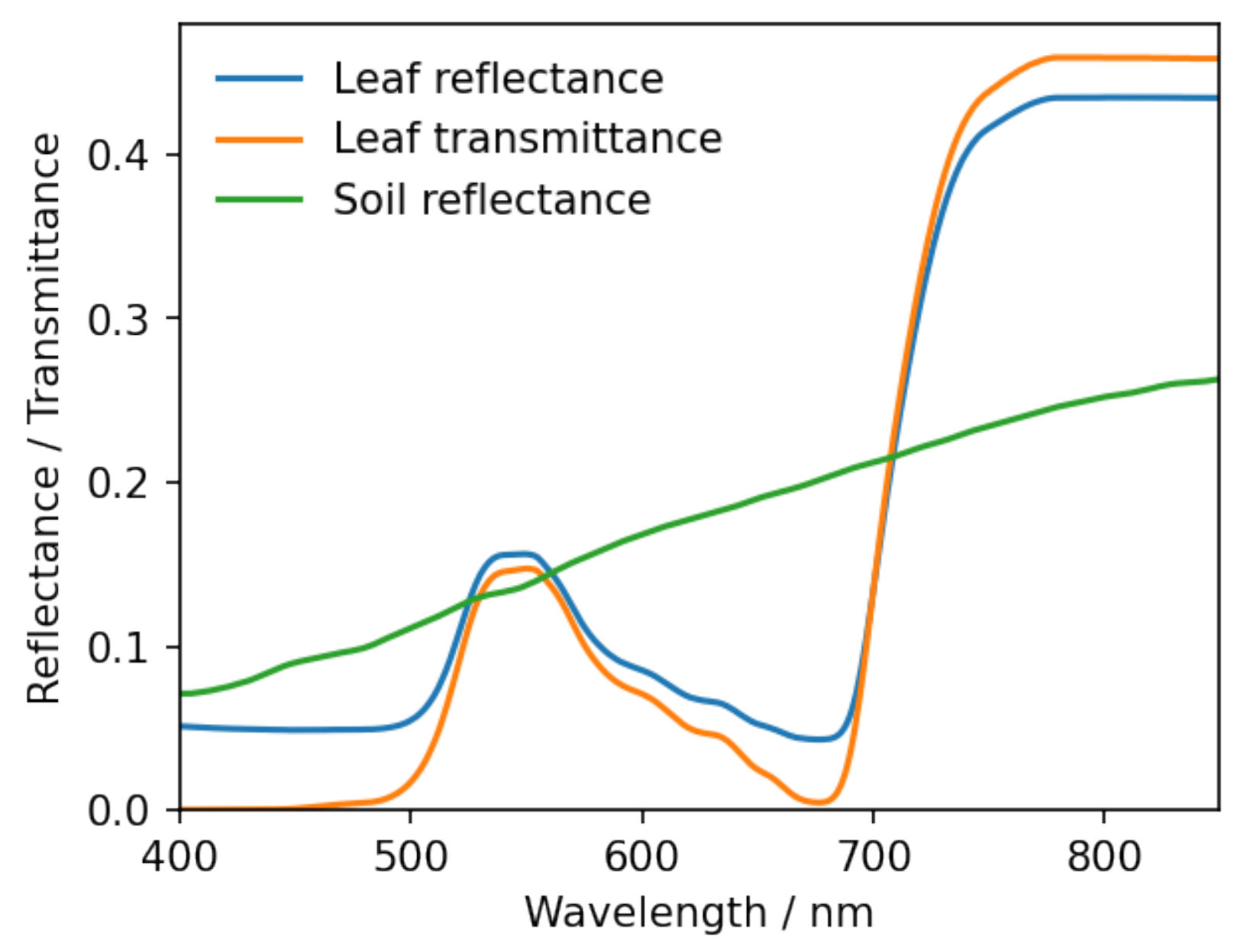
The simulation is driven by spectral and illumination conditions. These include leaf spectral properties like reflectance, transmittance, and EF-matrices simulated by Fluspect version 1.2 with the leaf parameters (Table 2), as well as the soil reflectance and solar spectral irradiance from both direct sunlight and diffused skylight. Figure 3 shows the components’ spectra of the abstract scenes, including the leaf reflectance, the leaf transmittance, and the soil reflectance.

3.2. Field Data about Soybean

The experiment took place at the Huailai Remote Sensing Test Site of the Chinese Academy of Sciences, situated in Huailai County, Hebei Province, China (40.349°N, 115.785°E). Simultaneous measurements of soybean leaves and canopy were carried out during the experiment. The data measured in the field or retrieved from the field-measured data for driving or evaluating the model include leaf spectral measurements, canopy structural measurements, and canopy spectral measurements. This experimental dataset was employed by [25] to test the effectiveness of the FluorWPS model, and we also use it to validate our model here.

3.2.1. Leaf Spectral Measurements

Leaf spectral data were obtained using a LI-COR 1800-12 system integrating sphere apparatus (LI-COR Inc., Lincoln, NE., USA) in conjunction with an ASD FieldSpec Pro spectroradiometer (by ASD Inc., Boulder, CO, USA) as depicted in Figure 4.
Then, the leaf biochemical parameters and EF-matrices were derived through a two-stage inversion process utilizing Fluspect as demonstrated by Zhao et al. [25].

3.2.2. Canopy Structural Measurements and Abstract Scene Construction

Canopy structures were measured destructively in a 1.5 × 1.5 m 2 plot. The average canopy height is about 90 cm. The LAI is about 3.0. The average leaf angle is about 30.4 ° and its standard deviation is 20.0 °.
According to the characteristics of the soybean canopy, it is assumed that leaves are evenly spread throughout. The scene created does not include stems and flowers. Leaves are approximated as triangle patches. A homogeneous canopy scene is generated with the same structural parameters as the soybean canopy.

3.2.3. Canopy Spectral Measurements

Spectral irradiance and radiance data under clear sky conditions were collected hourly between 09:30 and 14:30 (GMT + 8) on 15 September 2014 for soybeans. These spectral measurements were conducted at a height of 1.8 m above the ground in the nadir direction with a field of view of 25° using an AvaField-3 spectrometer (Avants Inc., located in Apeldoorn, the Netherlands) [25]. Then, the SIF spectrum spanning from 640 to 850 nm was retrieved using the fluorescence spectrum reconstruction (FSR) method [47].

3.3. Field Data about Corn

The ability of the proposed model to represent a range of canopy structures makes it an attractive tool for studying SIF distributions in realistic canopy settings. In this study, a corn canopy, including the structural models and their spectral characteristics, are used to construct an example scene. As a proof of concept, the application of fluorescence imaging and the diurnal variation of the SIF are considered.
Summer maize serves as a primary food crop and a major vegetation type in summer in Northern China. Modeling studies assist in uncovering the mechanisms that drive the distributions of SIF. The SIF simulations of the corn canopy lay a foundation for research on other crops.
The experiment was conducted at Luancheng Ecologic Experiment Station (37°53′ N, 114°41′ E, altitude 50.1 m), which is located in Hebei Province, China. Concurrent leaf and canopy measurements for corn were performed in July 2000.

3.3.1. Leaf and Stem Spectral Measurements

The components’ spectral data were measured using SE590 (Spectron Engineering Inc., Denver, CO, USA) equipped with an integrating sphere, including leaves and stems. The reflectance values of leaves on both sides and the transmittance were measured. It was found that the reflectance spectra from both sides are very close. Therefore, in the simulation, the reflectance values on both sides of each leaf were set to be the same. On the whole, due to the changes in the leaf structure and chemical composition between young leaves (the tender leaf and the first green leaf (from the top)) and other mature leaves, their transmittance and reflectance spectra are quite different, while the differences among other mature leaves are relatively small. Therefore, the measured reflectance and transmittance of young leaves, as well as the average reflectance and transmittance of other leaves, were chosen as the optical properties of corn leaves in the simulation (Figure 5). The reflectance of the soil is also presented in Figure 5 such that the optical properties of the corn scene are kept as much as possible, and the complexity of the input parameters is reduced.

3.3.2. Structural Measurements and Geometrically Explicit Canopy Generation

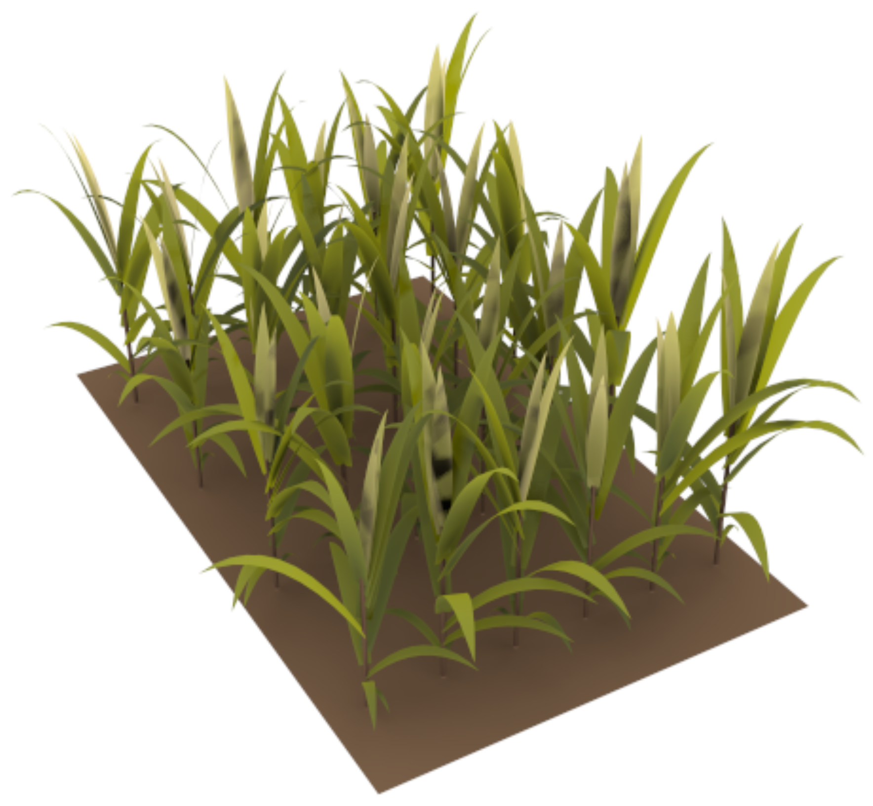
While conducting the measurements for spectral data, the structural data were measured, such as plant height, leaf width, leaf length, and leaf angle distribution. An efficient method with a digital imaging approach was developed by Wu et al. [48] to construct a geometrically explicit structure of the corn canopy. The true–virtual distance ratio is defined as the ratio between the true distance and the pixel distance on the image. This facilitates the conversion of image information into actual data. Using the data, the geometrically explicit structure of the corn canopy was constructed. The generated corn scene is shown in Figure 6. The corn is planted in rows with a distance between the rows of 60 cm, a mean width of the plants within the row of 25 cm, a mean plant height of 109.0 cm, and an LAI of 2.24, close to the measurements in the field.

4. Results

4.1. Comparison with the SCOPE Model

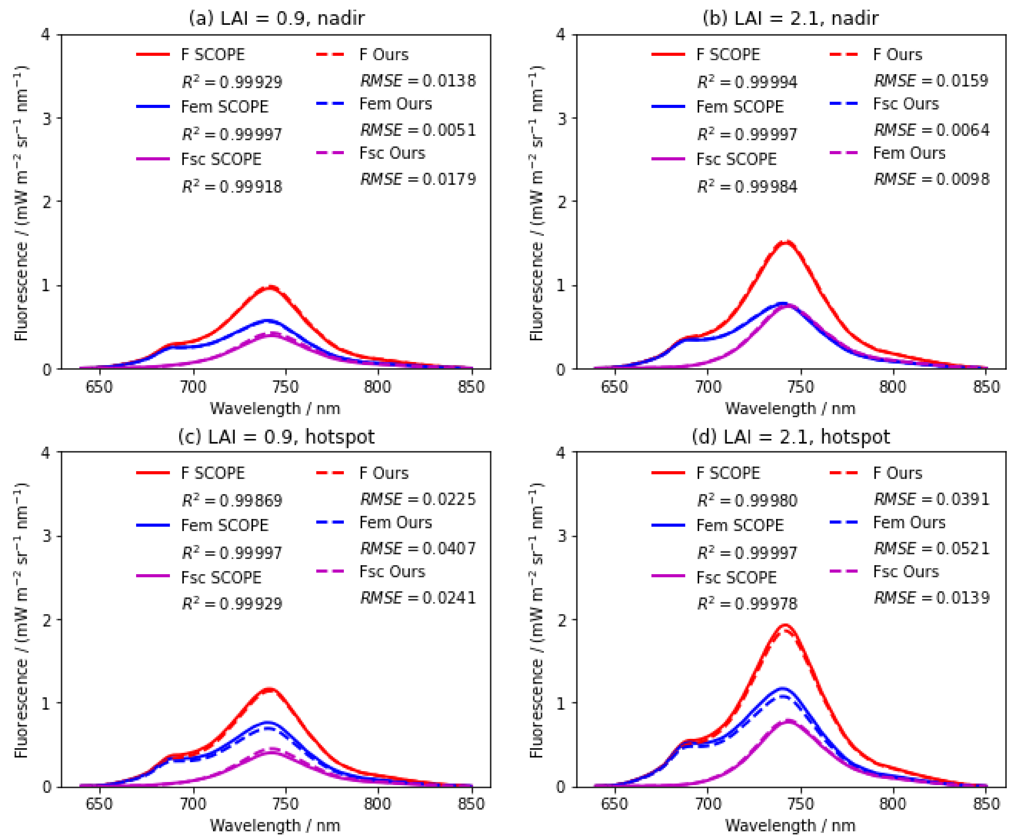
The proposed model is compared with the SCOPE (version 1.73) model based on the data in Section 3.1. For model comparisons, the structural and spectral input conditions for both models are kept as identical as possible. Homogeneous canopy scenes, as assumed in SCOPE, are generated using multiple polygons for the proposed model. The statistical parameters of the canopy scene are calculated for SCOPE. The spectral data are extracted from the SCOPE simulations. To evaluate the fluorescence distributions systematically, comparisons of both spectral and multi-angular SIF distributions are carried out. The spectral range spans from 640 nm to 850 nm in increments of 1 nm. The viewing zenith angle (VZA) ranges from 0° to 70° in steps of 10°, and the viewing azimuthal angle (VAA) varies from 0° to 350° in steps of 10°. The sun zenith angle (SZA) is set at 30° and the sun azimuth angle (SAA) at 140°.
The overall SIF detected by a sensor positioned at the top of the canopy can be categorized into two components: firstly, the portion emitted directly by the leaves and detected by the sensor without any obstruction (referred to as Fem), and secondly, the part of Fem that is scattered by both leaves and soil (referred to as Fsc). When combined, Fem and Fsc represent the total fluorescence (F) detected by the sensor. These three parts simulated by SCOPE and the proposed model are compared, respectively.

4.1.1. SIF Spectrum

Figure 7 displays the spectra of the total SIF and its components—emission part (Fem) and scattering part (Fsc)—in the nadir direction or hotspot, simulated by both the proposed model and the SCOPE model for two homogeneous canopies. The F spectra from both models exhibit the typical red and far-red peaks, approximately at 685 nm and 740 nm, respectively. As LAI increases, there is a general rise in F, particularly noticeable in the Near-Infrared (NIR) regions. Overall, the SIF predictions from the proposed model closely align with those from the SCOPE model across both canopies.

4.1.2. Angular SIF Distributions

Figure 8 displays the polar plots of F at wavelengths 685 nm and 740 nm, as well as Fsc at 740 nm for a simulated canopy LAI of 2.1, using both the proposed model and the SCOPE model.
In these plots, the central point represents a VZA of 0° (the nadir direction), with VZA values increasing radially outward. The VAA begins at the top and progresses clockwise, reaching 90° at the right. Due to the symmetric distribution with respect to the solar principal plane (PP), the values with VAA greater than SAA are copied from the corresponding value with VAA lower than SAA in the plots.
The SIFs at 685 nm and 740 nm, as simulated by both models, exhibit a bowl shape with a local maximum in the hotspot direction (Figure 8a,b,d,e). Bowl-shaped patterns, almost symmetric around the nadir, are observed in polar plots for Fsc (Figure 8g,h), indicating relatively weak anisotropy. The general forms of fluorescence distributions from both models are essentially identical. Moreover, all of the absolute differences are below 0.12 mW m−2 sr−1 nm−1 (Figure 8c,f,i), demonstrating good agreement between the fluorescence distributions of the two models.
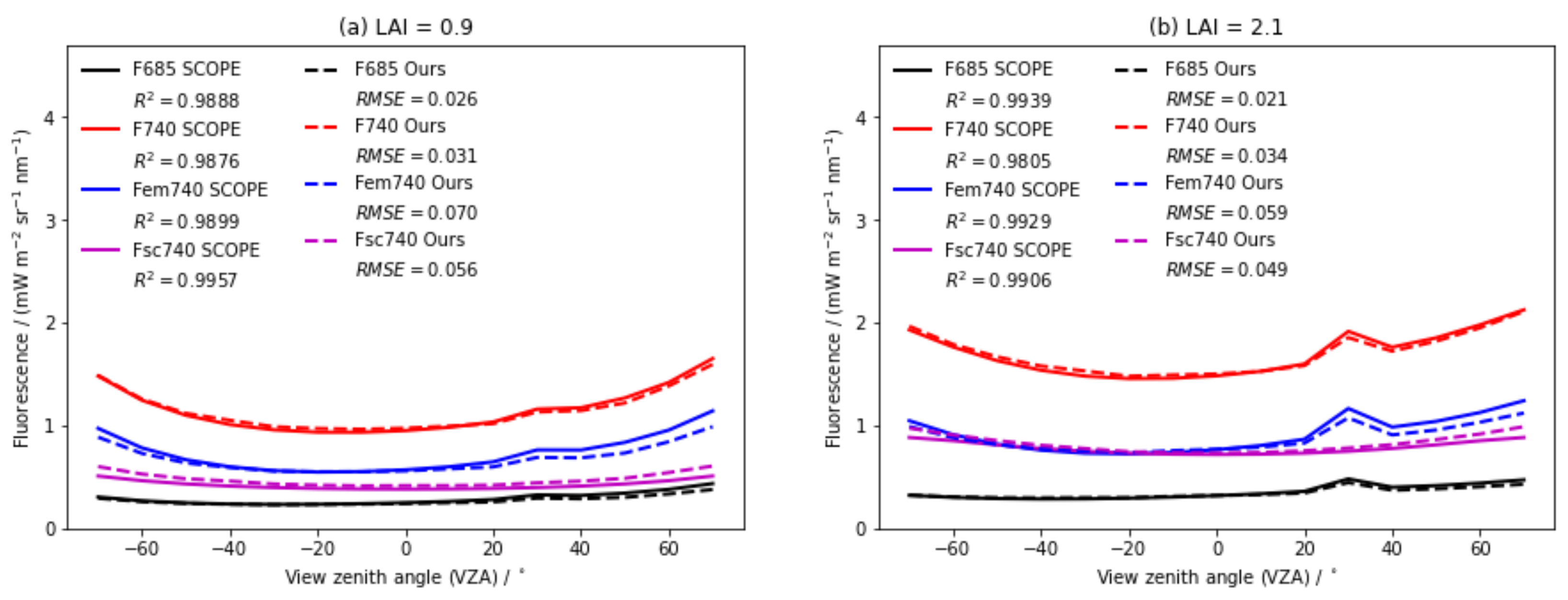
In Figure 9, a comparison is illustrated along the PP between the proposed model and the SCOPE model at 685 nm and 740 nm. Here, negative VZAs denote the forward direction, while positive VZAs represent the backward direction. A peak in the hotspot direction is observed for both models’ simulations in the fluorescence, excluding the scattering component. The results show good agreement between the two models.
Generally, the total fluorescence F at 685 and 740 nm simulated by the proposed model closely matches the results from the SCOPE model for low VZAs less than 20 degrees and high VZAs in the forward direction. And Fem and Fsc at 740 nm between the two models show good agreement for low VZAs across all canopy scenes, although there is a slight deviation observed for high VZAs. Fem simulated by the proposed model is a little lower than that by SCOPE for high VZAs, while Fsc is higher, enabling F(=Fem + Fsc) to agree with that by SCOPE. The slight deviation at high VZAs compared with SCOPE is also reported in Zhao et al. [25].
Correlation statistics for PP viewing angles (Table 3) demonstrate that the determination coefficients ( R 2 ) and root mean square errors (RMSEs) are higher than 0.98 and lower than 0.08 mW m−2 sr−1 nm−1, respectively, for both the red peak and far-red peak.

4.2. Comparison with Field Measurements

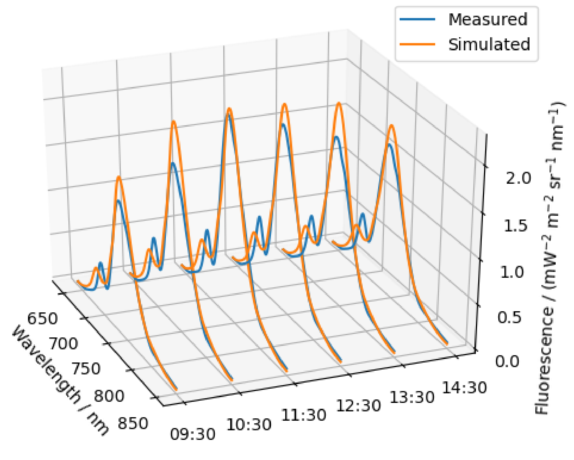
Six sets of paired datasets, involving both leaf and canopy measurements of soybean, were collected (Section 3.2). Figure 10 presents a comparison between the simulated SIF spectra generated by the proposed model and those reconstructed using the FSR method. Both the values and general shapes of the simulated SIF spectra match those of the reconstructed spectra over time, albeit with some noticeable differences. For the spectral range of 670–800 nm at 1 nm intervals, the coefficient of determination is 0.95, and the RMSE is 0.14 mW m−2 sr−1 nm−1 for the soybean canopy. Typical diurnal variations in SIF spectra, influenced by changes in incident irradiance, are also evident; they increase until mid-morning before declining.

5. Discussion

5.1. Model Application on the Impact of Row Structure on SIF Distributions

As illustrated in Figure 11, the spectral and angular SIF distributions for the row canopy are lower compared to those in the homogeneous scene. This finding is consistent with that of Zhao et al. [25]. This is due to the fact that a significant part of the row canopy in the nadir direction consists of soil between the rows, which does not emit fluorescence.
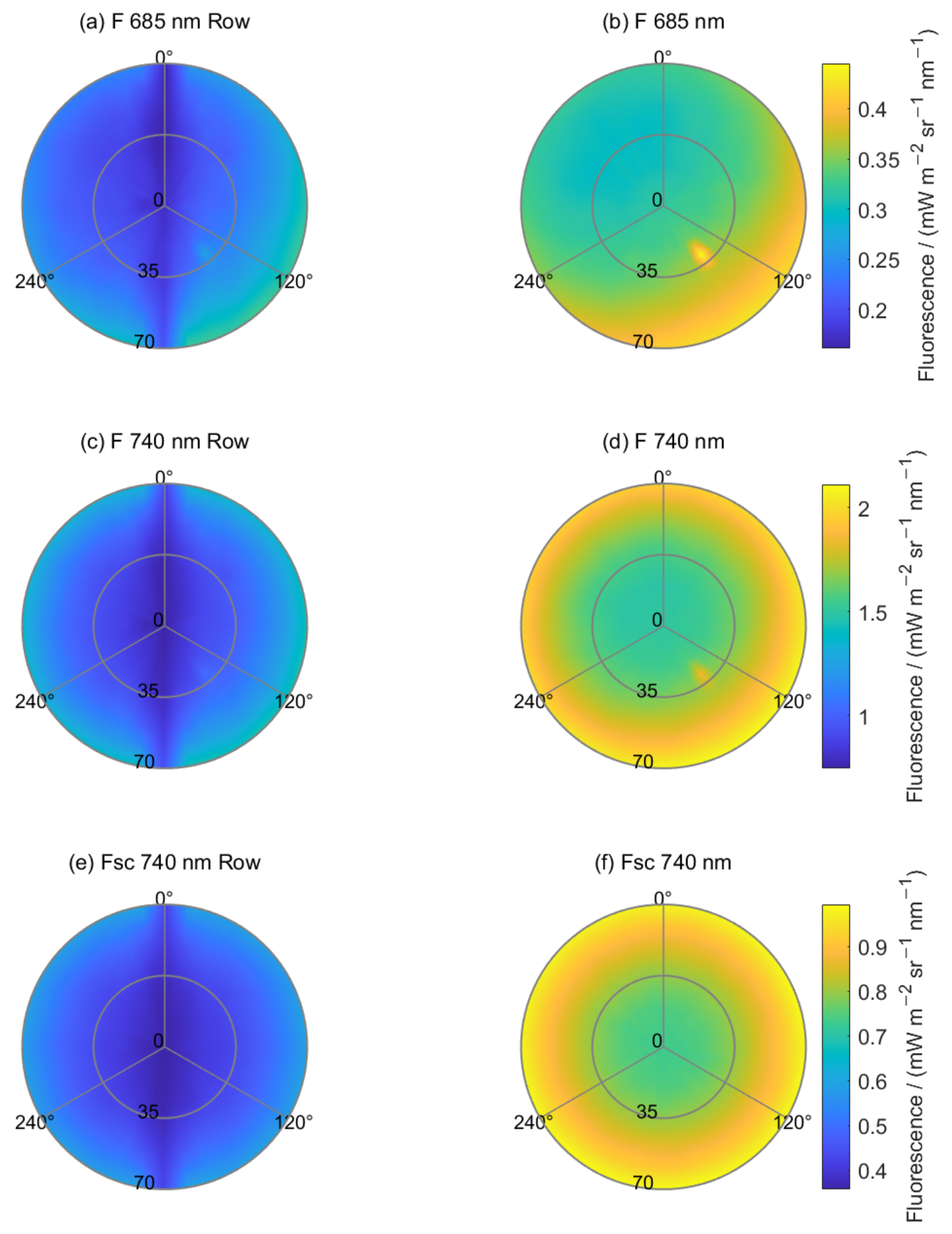
The influence of row structure is depicted in Figure 12. In the polar plots of fluorescence for the row scene (Figure 12a,c,e), a low-value stripe can be observed running roughly parallel to the row direction. This pattern is in line with those of previous studies [25,49]. This pattern is evident in both the emission and scattering components, resulting in an overall SIF that also displays a low-value stripe parallel to the row orientation. Conversely, the homogeneous scene demonstrates a bowl-shaped symmetric distribution relative to the PP. In this case, the emission component forms a bowl shape with a local maximum towards the hotspot direction within the PP, while the scattering component shows a nearly symmetric bowl-shaped distribution around the nadir. Consequently, this results in a bowl-shaped symmetric distribution with respect to the PP for homogeneous scenes (Figure 12b,d,f).
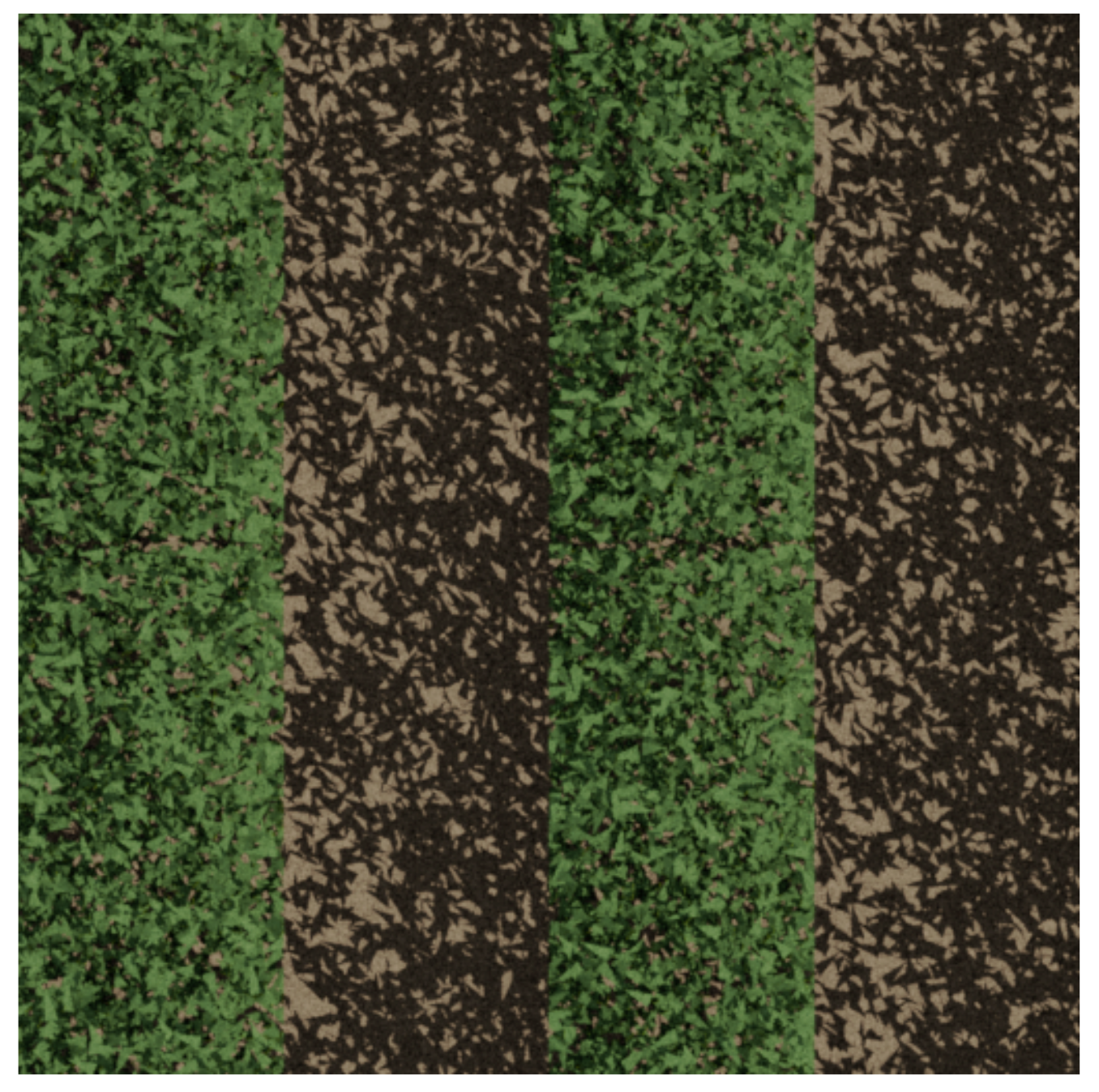
Variations in SIF appear across various aggregation levels in a simulated image of the row scene. Figure 13 illustrates how SIF extracted from the original high-resolution image changes with increasing pixel-aggregation levels. In Figure 13a, which shows the original SIF image, the canopy has high fluorescence values, and the ground has low values. In the canopy, the texture can be seen clearly due to the scattered leaves. There are low values on the left side, corresponding to the shaded leaves that can be seen in the natural color image (Figure 14) (recall that the SAA is 140°). From Figure 13b to Figure 13d, the resolution varies from high to low, and the texture becomes smooth. The resolutions are high enough to distinguish the vegetation from the ground. Figure 13e shows constant values because the pixel-aggregation level is high enough to aggregate the fluorescence from the canopy and the ground, and only average values are obtained, which are lower than the pure canopy pixel value, and higher than the pure ground pixel value.

5.2. Model Application on the Realistic Corn Scene

The ability of the proposed model to represent a range of canopy structures makes it attractive for studying SIF distributions in realistic canopy settings. As a proof of concept, the application of fluorescence imaging and the diurnal variation of the SIF is considered.

5.2.1. Fluorescence Imaging

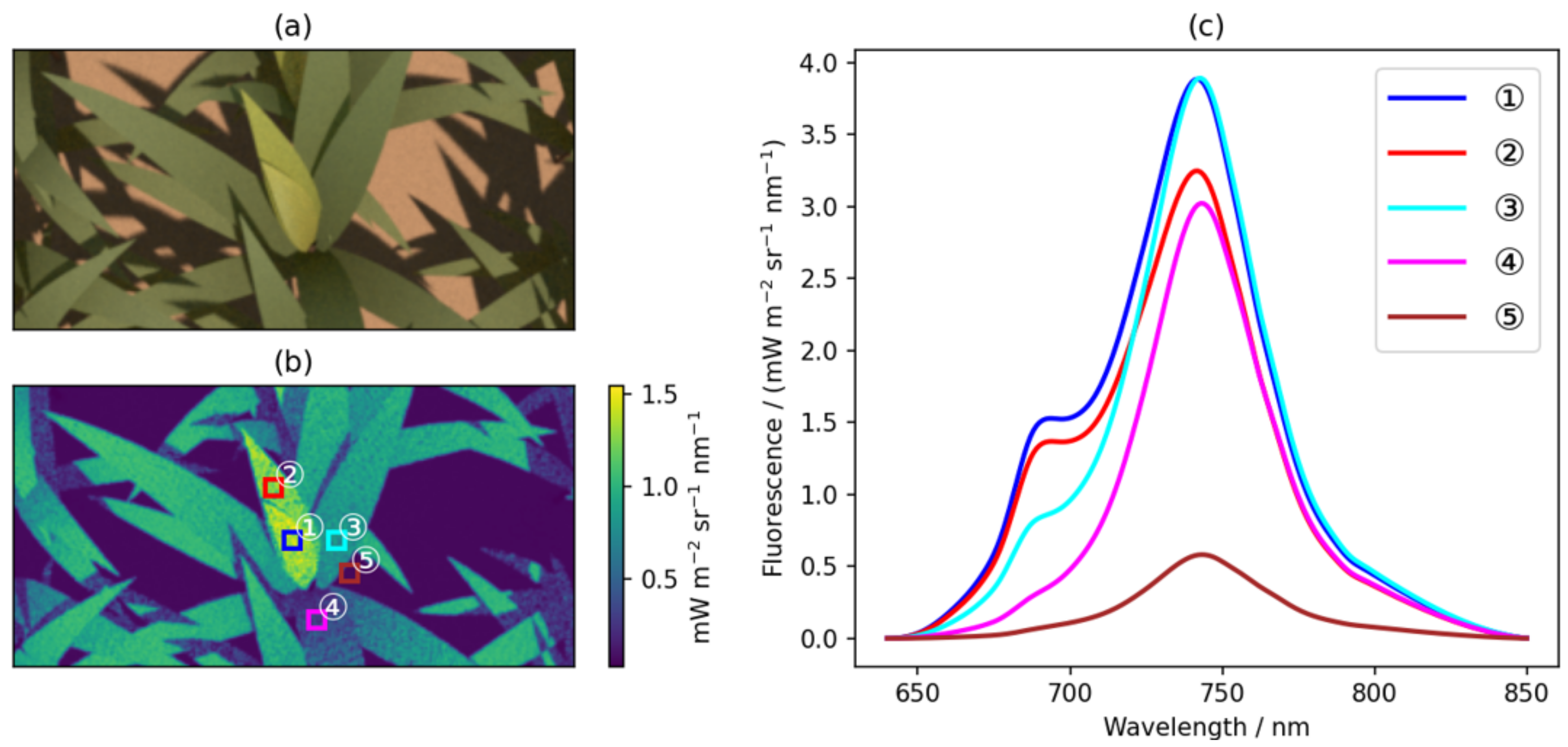
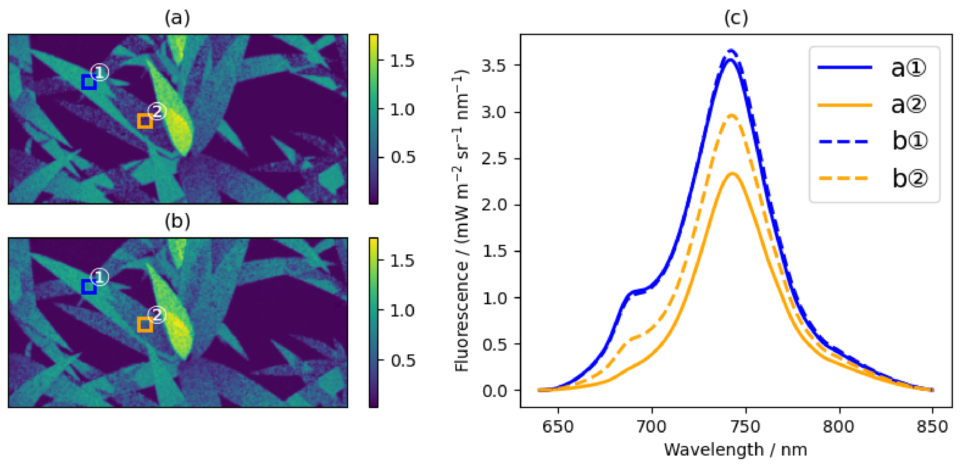
A fluorescence image of the realistic corn scene (Section 3.3) at noon (12:00 GMT + 8) is shown in Figure 15. The sun zenith angle is 18°, and the sun azimuth angle is 156°. Figure 15b highlights five samples taken from different leaves and positions within the canopy. The five samples demonstrate the variability in fluorescence across the canopy. Sample (1) is from a tender leaf, sample (2) is from the first green leaf from the top, sample (3) is from a sunlit green leaf, sample (4) is from a shaded green leaf, and sample (5) is from the ground. Figure 15c shows the simulated SIF spectra for these five samples. The spectra for samples (1)–(4), which are from leaves, exhibit the typical red and far-red peaks around 685 nm and 740 nm, respectively. Comparing the sunlit leaf samples, the tender leaf (sample (1)) has the highest SIF at 685 nm, followed by the first green leaf (sample (2)) and then the sunlit green leaf (sample (3)). This matches the retrieved chlorophyll AB contents of 7, 12, and 40 μg cm−2 or these three leaves, respectively. However, at 740 nm, the order is different, with the first green leaf (sample 2) having the lowest SIF value among the three sunlit leaf samples. This highlights that the relationship between SIF and chlorophyll content is not always straightforward as discussed further in the literature [50]. Since the focus of this article is not on the detailed relationship between SIF and leaf biochemistry, we will not delve deeply into that topic here. The SIF values of sample (4) taken from the shaded green leaf are lower than those of the sunlit green leaf (sample 3). These differences are primarily caused by the illumination conditions (Figure 15a). To make the description sophisticated, an evaluation of leaf-level illumination is conducted. For measurement purposes, an ideal diffuse reflectance target is attached to the sample as shown in Figure 16 [39]. Then, the retrieved PAR values for samples (3) and (4) are about 1066 and 241 μmol m−2s−1, respectively. The leaf position that receives more incident energy, like the sunlit leaves, will emit higher fluorescence. The SIF values for the sample (5) taken from the ground are the lowest among all the samples. This is because the ground itself does not emit SIF. The values measured for the ground sample (5) represent the scattered fluorescence from the surrounding vegetation and soil. Compared to the leaf samples, the red peak around 685 nm is less pronounced in the ground sample (5) spectrum. This can be explained by the relatively low SIF values and the higher absorption of red wavelengths by the plant elements within the scene.
Moreover, the variation of the SIF on leaves caused by shadows can be clearly seen in Figure 15b, which includes the difference between samples (3) and (4). This demonstrates that the radiation information in the scene is stored independently of the underlying geometry or polygons. If the radiation representation were tightly coupled to the polygonal structure, the SIF values within a single polygon would be identical, and the fine-scale variation caused by shadows may not be as pronounced as that shown in the figure. The versatile nature of the model’s decoupled representation of radiation and geometry is a key strength. It allows the model to better capture the complex and heterogeneous structure of real-world canopy systems.
By resolving these subtle differences in fluorescence emission, even within the same leaf or canopy element, the model provides a more realistic and detailed representation of the radiative transfer processes. This enables more accurate quantification and analysis of the underlying photosynthetic activity, which has important implications for remote sensing, precision agriculture, and other applications that rely on understanding the canopy’s functional dynamics.

5.2.2. SIF Images under Different Natural Light Conditions

Examples of simulated SIF images at 685 nm at 10:30 under different light conditions of the realistic corn scene are shown in Figure 17. Figure 17a,b depict the SIF under a clear sky and a slightly hazy day with more isotropic scattering [51], respectively. Samples from the SIF images are used to illustrate the fluorescence differences between the two light conditions.
Samples (a1) and (b1) are from the same sunlit leaf position, while (a2) and (b2) are from the same shaded leaf position but under different light conditions. Figure 17c shows the SIF spectra of these samples. As expected, the SIF values of sunlit samples (a1) and (b1) are higher than those of shaded samples (a2) and (b2), consistent with the findings in Section 5.2.1. Interestingly, the SIF values of sunlit samples (a1) and (b1) are nearly identical, despite the different input light conditions. However, the SIF values of shaded sample (a2) are lower than those of shaded sample (b2). This can be attributed to the differences in the illumination conditions—the shadow appears lighter in color in Figure 17b under the slightly hazy conditions, allowing more scattered light energy to reach the shaded leaf and resulting in higher fluorescence emission.
These results demonstrate the model’s capability to simulate the subtle contrasts in fluorescence imaging caused by varying illumination conditions. This versatility is a highly attractive feature, as it enables the study of realistic SIF distributions in complex canopy structures.

5.2.3. Diurnal Variation of the SIF

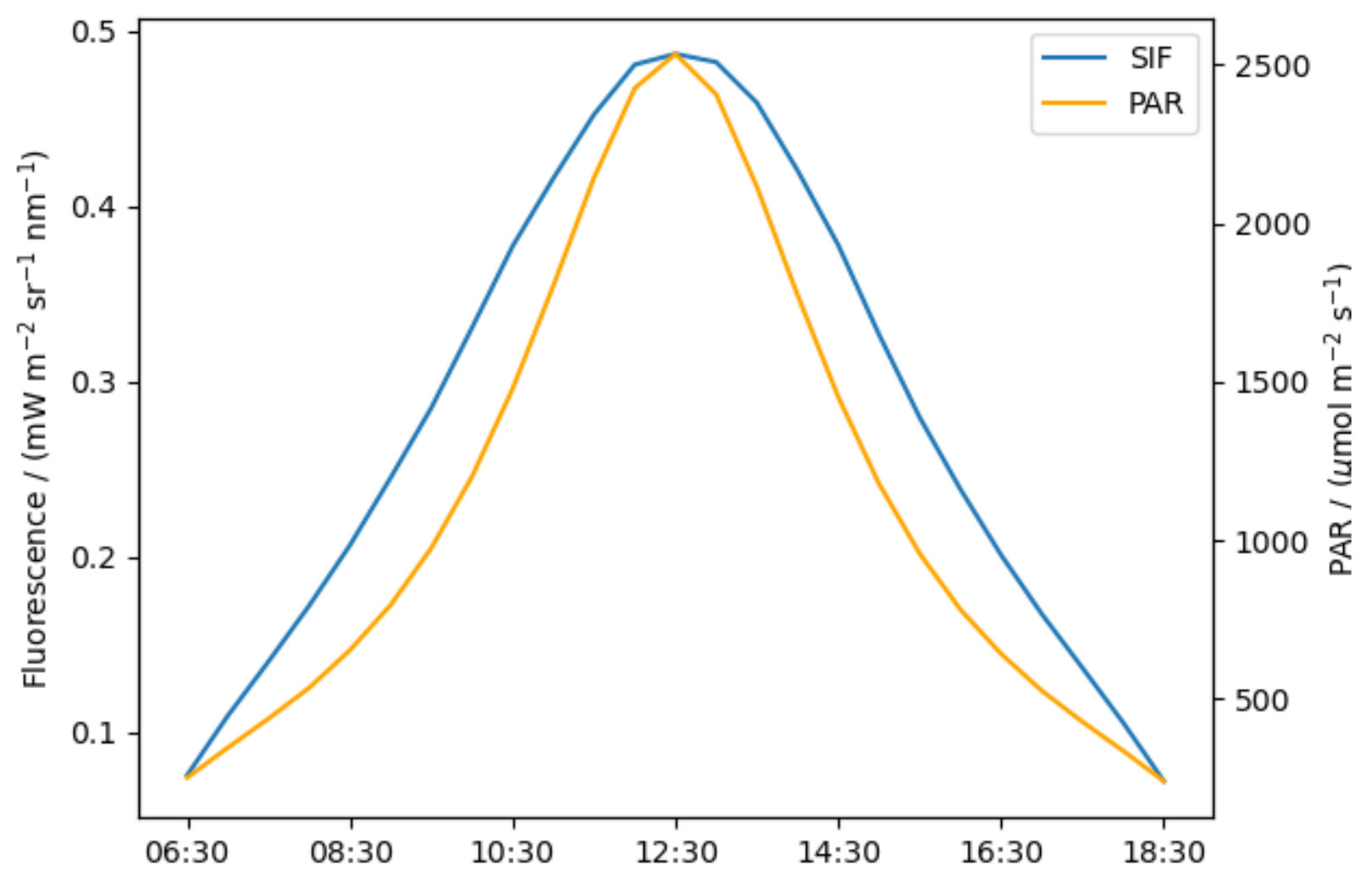
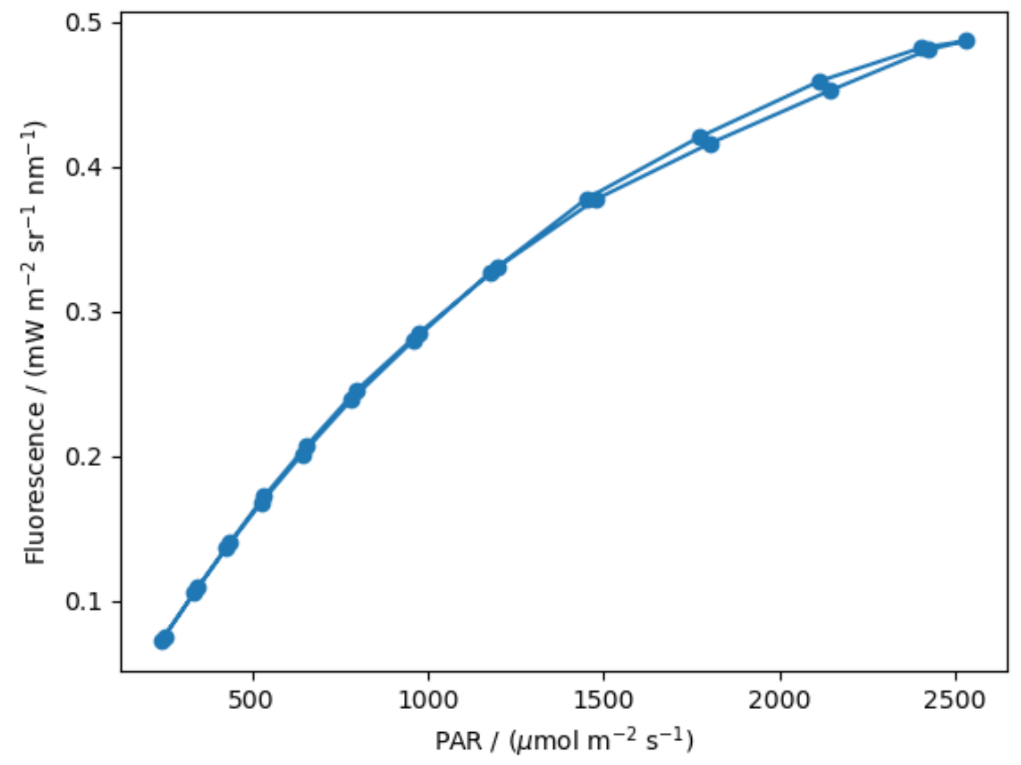
The solar spectral irradiance distributions were simulated at 30-min intervals from 06:30 to 18:30 (GMT + 8) using MODTRAN 5.2.2, representing a typical midsummer day with a visibility of 23 km. The diurnal variation of the Photosynthetically Active Radiation (PAR) retrieved from these simulated data is shown in Figure 18. These PAR data were then used to drive the simulation of the diurnal variation in Sun-Induced Fluorescence (SIF) for the realistic corn scene. The typical temporal patterns can be observed, with both the SIF at 685 nm and the PAR increasing until noon and then decreasing in a roughly symmetrical manner on a clear day. However, the slopes of the two curves are not always identical. Consequently, the graph of SIF as a function of PAR is not a straight line (Figure 19). This can be explained by the non-linear relationship between the leaf fluorescence response and light level as accounted for by the correction factor φ in the model. The φ factor is a non-linear function of PAR according to the formulas provided in Appendix A. This observed non-linearity between SIF and PAR highlights the importance of the model’s ability to capture the complex, dynamic interplay between the illumination conditions and leaf-level fluorescence response. Such nuanced relationships are crucial for accurately simulating and interpreting the spatiotemporal patterns of SIF in realistic canopy scenarios.
The high-resolution fluorescence imaging capabilities of the model can be leveraged to examine the diurnal variation of SIF at different positions and horizontal levels within the canopy scene. Figure 20 shows the diurnal variations of SIF at 685 nm for five samples within the realistic corn scene. In contrast to the smooth, symmetric diurnal patterns observed for the overall canopy SIF in Figure 18, most of the individual sample curves exhibit more irregular, asymmetric behavior. This can be explained by the fact that the canopy-level SIF is an aggregation of signals from across the scene, where local variations in illumination conditions tend to average out. The diurnal trends in canopy SIF are predominantly driven by the diurnal PAR variation, resulting in the symmetry observed in Figure 18.
However, the individual sample SIF diurnal patterns are more heavily influenced by the heterogeneous local illumination conditions within the canopy. Consistent with the fluorescence imaging analysis in Section 5.2.1, the tender leaf sample (1) displays the highest SIF, while the ground sample (5) having the lowest. The timing of the SIF peaks also varies, with samples (1) and (2) peaking around 10:30, while samples (3) and (4) peak around 13:30. This phase delay can be attributed to differences in leaf angle distributions, as the leaves face the sun at different times of the day.
Additionally, the sample SIF values can decrease steeply and exhibit non-smooth behavior, particularly for lower-level samples affected by shadows cast by upper leaves as seen for sample (3) around 14:30 and in Figure 21e,f. This highlights how leaves at lower horizontal positions within the canopy tend to be impacted by shading from above. Finally, the ground sample (5) shows a relatively smooth, symmetric diurnal SIF pattern, as the ground itself does not emit fluorescence, and the observed signal is primarily due to scattered fluorescence.
Overall, this analysis demonstrates the importance of accounting for the heterogeneous illumination conditions and their impact on the spatiotemporal variations of SIF within a realistic canopy scene.
The examples of SIF images from the simulation of the realistic corn scene, shown in Figure 21, capture the typical temporal variations in the output SIF at 685 nm over the course of the day. These images clearly demonstrate the changes in the shadows cast within the canopy, driven by the evolving sun direction. Additionally, there are gradual changes in SIF across the bowed leaves. The key point is that the model’s use of a decoupled representation, rather than the radiation representation tightly coupled to the polygonal structure, allows it to capture the subtle variations in SIF caused by complex illumination patterns within the canopy as illustrated in Figure 21. The results presented here show that the model has the capability to simulate the nuanced contrasts in fluorescence imaging driven by evolving illumination conditions, highlighting the attractiveness of this tool for studying SIF distributions in realistic canopy environments.

5.3. Perspectives

The proposed model takes into account the spectral range, structural effects, and temporal patterns, which are key aspects of fluorescence research and applications [19,52].
The findings of the impact of row structure on SIF distributions are consistent with those of Zhao et al. [25], who demonstrated that the canopy structure significantly influences the spectral and directional distributions of SIF, resulting in greater SIF anisotropy compared to a homogeneous canopy with a similar leaf area index and leaf angle distribution. The row effect of SIF at varying view directions identified a low-value stripe that runs approximately parallel to the row orientation in the polar plot of SIF. This pattern is consistent with the findings from other models, including FluorWPS [25] and FLiES-SIF [28,49]. Ref. Morozumi et al. [49], using FLiES-SIF, investigated the effect of row orientation on diurnal simulated SIF variations. The proposed model also showed the ability to simulate diurnal SIF; however, a more sophisticated investigation on this comprehensive topic, the row effect on diurnal SIF, has not been conducted in this study.
The independent representation of radiation information in the model allows for the capture of subtle variations in SIF due to complex illumination patterns within the canopy, which is a key advantage over approaches relying on how the polygons are tessellated. This capability makes the model a valuable tool for investigating the spatial and temporal patterns of photosynthesis in realistic crop canopy scenarios.
Fluorescence imaging provides a non-destructive method for vegetation monitoring. Investigations that assess vegetation monitoring techniques using three-dimensional radiative transfer modeling are particularly insightful [53]. Simulations of fluorescence images with the proposed model revealed that the fluorescence heterogeneity can be generated by the leaf scene modeling with different light illumination and leaf chlorophyll content. Additionally, pulse amplitude modulated (PAM) fluorescence is a viable technique for imaging fluorescence [54]. However, it is important to note that PAM fluorescence requires the active regulation of light conditions [55]. Furthermore, PAM images illustrate the heterogeneity of chloroplasts within leaves [33]. Therefore, when collaborating between the PAM fluorescence technique and the three-dimensional fluorescence radiative transfer modeling, these factors should be taken into account.
The proposed model integrates input from Fluspect and incorporates the dependence of the fluorescence correction factor on the incident photosynthetic active radiation levels. However, the proposed model does not currently include calculations for photosynthesis and energy balance, unlike the SCOPE model [24]. Future considerations should include incorporating other light sources and environmental factors, as well as coupling physiological processes in the three-dimensional fluorescence model. These considerations draw inspiration from studies such as Linn et al. [54] and Van Wittenberghe et al. [52], along with advancements in other 3D models, including DART [26,56], FLiES-SIF [28,49], and FluorWPS [25,57].

6. Conclusions

In this work, we have proposed a radiative transfer simulation model that uses the Monte Carlo ray-tracing method to quantitatively compute canopy sun-induced fluorescence (SIF). A key innovation of the model is the decoupling of the radiation representation from the geometric representation of the scene. By using a point-based approach for the radiation, the proposed model eliminates the need for tessellating the geometry, enabling a more flexible and versatile representation of the canopy structure. Through systematic evaluations, the proposed model was shown to closely reproduce the temporal SIF spectra, which were comparable to field-measured data. Comparisons with the established SCOPE model further enhanced the confidence in the accuracy and reliability of both modeling approaches.
Furthermore, we demonstrated the versatile nature of the proposed model’s canopy representation by applying it to study the impact of row structure on SIF and fluorescence imaging. This capability makes the proposed model a highly attractive tool for investigating SIF distributions in realistic, heterogeneous canopy environments. The flexibility and realism afforded by the proposed model offer promising opportunities for advancing our understanding of various plant and ecosystem processes, such as crop yield estimation, vegetation stress monitoring, and quantification of photosynthetic capabilities. As such, this model presents an important step forward in the field of SIF modeling and its applications in remote sensing and precision agriculture.

Author Contributions

Funding acquisition, D.X.; investigation: Y.L.; writing—original draft, Y.L.; writing—review and editing, D.X. and J.Q.; supervision, G.Y. and X.M. All authors have read and agreed to the published version of the manuscript.

Funding

The work is funded by the National Natural Science Foundation of China (Grant No. 42071304 and 42471376) and the National Key Research and Development Program of China (Grant No. 2022YFB3903304).

Data Availability Statement

The data presented in this study are available on request from the corresponding author due to privacy.

Acknowledgments

The authors thank Feng Zhao for providing the field experiment data; Xiaohan Dong for processing the measured data of the corn scene; Bin Sun for generating and processing the radiation data used in the simulations of the corn scene; and Guofang Miao for giving useful suggestions.

Conflicts of Interest

The authors declare no conflicts of interest.

Appendix A. Dependence of the Fluorescence Correction Factor on Incident Photosynthetic Active Radiation Level

The photosynthetic active radiation (PAR) light level dependence model of leaf fluorescence by Rosema et al. [38] is applied to calculate the fluorescence correction factor φ . This section starts by showing how to calculate the fluorescence correction factor φ , and then summarizes the PAR.
To calculate the fluorescence correction factor φ , three equations are used as summarized in Miller et al. [7] and Zhao et al. [25], given by
φ P 0 = φ P 0 1 + b P P A R ( 1 φ P 0 φ F 0 ) ,
where φ P 0 is the proportion of energy dedicated to photosynthesis in the open photosystems equal to 0.82 . b P is called the heat dissipation constant, which is recommended at a value of 0.0035 , and φ F 0 is the corresponding fluorescence fraction equal to 0.01 [38].
The photosynthetic quantum yield φ P is given by
φ P = φ P 0 1 + r e φ P 0 P A R ,
where r e is the electron transport resistance, which is recommended at a value of 0.005 [38].
The fluorescence correction factor φ is calculated as
φ = φ P 0 φ P 0 1 φ P 1 φ P 0 .
In order to apply this model, the flux needs to be transformed into photon flux densities in μmol m−2s−1 and then integrated across the PAR wavelength range of 400–700 nm. The following equation is used for this conversion:
P A R = 10 3 h c N A Λ E λ d λ ,
where E is a radiant flux density (irradiance) in mW   m 2   nm 1 , and the wavelength λ is also expressed in nm . The product hc = 6.626 070 × 10−34 J s × 299 792 458 ms−1 = 1.986 44 × 10−16 Jnm, which is Planck’s constant times the speed of light. The constant NA = 6.022 × 10²³ mol−1 is Avogadro’s number. And Λ means that the range is from 400 nm to 700 nm.

References

  1. Glassner, A. Principles of Digital Image Synthesis; Elsevier: Amsterdam, The Netherlands, 1995. [Google Scholar] [CrossRef]
  2. Louis, J.; Cerovic, Z.G.; Moya, I. Quantitative Study of Fluorescence Excitation and Emission Spectra of Bean Leaves. J. Photochem. Photobiol. B Biol. 2006, 85, 65–71. [Google Scholar] [CrossRef] [PubMed]
  3. Oerke, E.C. Remote Sensing of Diseases. Annu. Rev. Phytopathol. 2020, 58, 225–252. [Google Scholar] [CrossRef] [PubMed]
  4. Goetz, A.F.H.; Vane, G.; Solomon, J.E.; Rock, B.N. Imaging Spectrometry for Earth Remote Sensing. Science 1985, 228, 1147–1153. [Google Scholar] [CrossRef] [PubMed]
  5. Milton, E.J. Review Article Principles of Field Spectroscopy. Int. J. Remote Sens. 1987, 8, 1807–1827. [Google Scholar] [CrossRef]
  6. Aasen, H.; Van Wittenberghe, S.; Sabater Medina, N.; Damm, A.; Goulas, Y.; Wieneke, S.; Hueni, A.; Malenovský, Z.; Alonso, L.; Pacheco-Labrador, J.; et al. Sun-Induced Chlorophyll Fluorescence II: Review of Passive Measurement Setups, Protocols, and Their Application at the Leaf to Canopy Level. Remote Sens. 2019, 11, 927. [Google Scholar] [CrossRef]
  7. Miller, J.; Berger, M.; Goulas, Y.; Jacquemoud, S.; Louis, J.; Mohammed, G.; Moise, N.; Moreno, J.; Moya, I.; Pedros, R.; et al. Development of a Vegetation Fluorescence Canopy Model; Technical Report; ESTEC: Noordwijk, The Netherlands, 2005. [Google Scholar]
  8. Zhang, Y.; Xiao, X.; Jin, C.; Dong, J.; Zhou, S.; Wagle, P.; Joiner, J.; Guanter, L.; Zhang, Y.; Zhang, G.; et al. Consistency between Sun-Induced Chlorophyll Fluorescence and Gross Primary Production of Vegetation in North America. Remote Sens. Environ. 2016, 183, 154–169. [Google Scholar] [CrossRef]
  9. Mohammed, G.H.; Colombo, R.; Middleton, E.M.; Rascher, U.; van der Tol, C.; Nedbal, L.; Goulas, Y.; Pérez-Priego, O.; Damm, A.; Meroni, M.; et al. Remote Sensing of Solar-Induced Chlorophyll Fluorescence (SIF) in Vegetation: 50 Years of Progress. Remote Sens. Environ. 2019, 231, 111177. [Google Scholar] [CrossRef] [PubMed]
  10. Joiner, J.; Yoshida, Y.; Vasilkov, A.P.; Yoshida, Y.; Corp, L.A.; Middleton, E.M. First Observations of Global and Seasonal Terrestrial Chlorophyll Fluorescence from Space. Biogeosciences 2011, 8, 637–651. [Google Scholar] [CrossRef]
  11. Frankenberg, C.; Fisher, J.B.; Worden, J.; Badgley, G.; Saatchi, S.S.; Lee, J.E.; Toon, G.C.; Butz, A.; Jung, M.; Kuze, A.; et al. New Global Observations of the Terrestrial Carbon Cycle from GOSAT: Patterns of Plant Fluorescence with Gross Primary Productivity: Chlorophyll Fluorescence from Space. Geophys. Res. Lett. 2011, 38, L17706. [Google Scholar] [CrossRef]
  12. Frankenberg, C.; O’Dell, C.; Berry, J.; Guanter, L.; Joiner, J.; Köhler, P.; Pollock, R.; Taylor, T.E. Prospects for Chlorophyll Fluorescence Remote Sensing from the Orbiting Carbon Observatory-2. Remote Sens. Environ. 2014, 147, 1–12. [Google Scholar] [CrossRef]
  13. Köhler, P.; Frankenberg, C.; Magney, T.S.; Guanter, L.; Joiner, J.; Landgraf, J. Global Retrievals of Solar-Induced Chlorophyll Fluorescence with TROPOMI: First Results and Intersensor Comparison to OCO-2. Geophys. Res. Lett. 2018, 45, 10,456–10,463. [Google Scholar] [CrossRef] [PubMed]
  14. Du, S.; Liu, L.; Liu, X.; Zhang, X.; Zhang, X.; Bi, Y.; Zhang, L. Retrieval of Global Terrestrial Solar-Induced Chlorophyll Fluorescence from TanSat Satellite. Sci. Bull. 2018, 63, 1502–1512. [Google Scholar] [CrossRef] [PubMed]
  15. Porcar-Castell, A.; Tyystjärvi, E.; Atherton, J.; van der Tol, C.; Flexas, J.; Pfündel, E.E.; Moreno, J.; Frankenberg, C.; Berry, J.A. Linking Chlorophyll a Fluorescence to Photosynthesis for Remote Sensing Applications: Mechanisms and Challenges. J. Exp. Bot. 2014, 65, 4065–4095. [Google Scholar] [CrossRef] [PubMed]
  16. Moreno, J.F.; Asner, G.P.; Bach, H.; Belenguer, T.; Bell, A.; Buschmann, C.; Calera, A.; Calpe, J.; Campbell, P.; Cecchi, G.; et al. FLuorescence EXplorer (FLEX): An Optimised Payload to Map Vegetation Photosynthesis from Space. In Proceedings of the 57th International Astronautical Congress, Valencia, Spain, 2–6 October 2006. [Google Scholar] [CrossRef]
  17. Rascher, U.; Alonso, L.; Burkart, A.; Cilia, C.; Cogliati, S.; Colombo, R.; Damm, A.; Drusch, M.; Guanter, L.; Hanus, J.; et al. Sun-Induced Fluorescence—A New Probe of Photosynthesis: First Maps from the Imaging Spectrometer HyPlant. Glob. Change Biol. 2015, 21, 4673–4684. [Google Scholar] [CrossRef]
  18. Pinto, F.; Damm, A.; Schickling, A.; Panigada, C.; Cogliati, S.; Müller-Linow, M.; Ballvora, A.; Rascher, U. Sun-Induced Chlorophyll Fluorescence from High-Resolution Imaging Spectroscopy Data to Quantify Spatio-Temporal Patterns of Photosynthetic Function in Crop Canopies. Plant Cell Environ. 2016, 39, 1500–1512. [Google Scholar] [CrossRef]
  19. Pinto, F.; Müller-Linow, M.; Schickling, A.; Cendrero-Mateo, M.; Ballvora, A.; Rascher, U. Multiangular Observation of Canopy Sun-Induced Chlorophyll Fluorescence by Combining Imaging Spectroscopy and Stereoscopy. Remote Sens. 2017, 9, 415. [Google Scholar] [CrossRef]
  20. Jiang, Y.; Snider, J.L.; Li, C.; Rains, G.C.; Paterson, A.H. Ground Based Hyperspectral Imaging to Characterize Canopy-Level Photosynthetic Activities. Remote Sens. 2020, 12, 315. [Google Scholar] [CrossRef]
  21. Araus, J.L.; Kefauver, S.C.; Zaman-Allah, M.; Olsen, M.S.; Cairns, J.E. Translating High-Throughput Phenotyping into Genetic Gain. Trends Plant Sci. 2018, 23, 451–466. [Google Scholar] [CrossRef]
  22. Watt, M.; Fiorani, F.; Usadel, B.; Rascher, U.; Muller, O.; Schurr, U. Phenotyping: New Windows into the Plant for Breeders. Annu. Rev. Plant Biol. 2020, 71, 689–712. [Google Scholar] [CrossRef]
  23. Bendig, J.; Malenovsky, Z.; Gautam, D.; Lucieer, A. Solar-Induced Chlorophyll Fluorescence Measured from an Unmanned Aircraft System: Sensor Etaloning and Platform Motion Correction. IEEE Trans. Geosci. Remote Sens. 2020, 58, 3437–3444. [Google Scholar] [CrossRef]
  24. van der Tol, C.; Verhoef, W.; Timmermans, J.; Verhoef, A.; Su, Z. An Integrated Model of Soil-Canopy Spectral Radiances, Photosynthesis, Fluorescence, Temperature and Energy Balance. Biogeosciences 2009, 6, 3109–3129. [Google Scholar] [CrossRef]
  25. Zhao, F.; Dai, X.; Verhoef, W.; Guo, Y.; van der Tol, C.; Li, Y.; Huang, Y. FluorWPS: A Monte Carlo Ray-Tracing Model to Compute Sun-Induced Chlorophyll Fluorescence of Three-Dimensional Canopy. Remote Sens. Environ. 2016, 187, 385–399. [Google Scholar] [CrossRef]
  26. Gastellu-Etchegorry, J.P.; Lauret, N.; Yin, T.; Landier, L.; Kallel, A.; Malenovsky, Z.; Bitar, A.A.; Aval, J.; Benhmida, S.; Qi, J.; et al. DART: Recent Advances in Remote Sensing Data Modeling with Atmosphere, Polarization, and Chlorophyll Fluorescence. IEEE J. Sel. Top. Appl. Earth Obs. Remote Sens. 2017, 10, 2640–2649. [Google Scholar] [CrossRef]
  27. Hernández-Clemente, R.; North, P.R.J.; Hornero, A.; Zarco-Tejada, P.J. Assessing the Effects of Forest Health on Sun-Induced Chlorophyll Fluorescence Using the FluorFLIGHT 3-D Radiative Transfer Model to Account for Forest Structure. Remote Sens. Environ. 2017, 193, 165–179. [Google Scholar] [CrossRef]
  28. Sakai, Y.; Kobayashi, H.; Kato, T. FLiES-SIF Ver. 1.0: Three-dimensional Radiative Transfer Model for Estimating Solar Induced Fluorescence. Geosci. Model Dev. 2020. preprint. [Google Scholar] [CrossRef]
  29. Verrelst, J.; van der Tol, C.; Magnani, F.; Sabater, N.; Rivera, J.P.; Mohammed, G.; Moreno, J. Evaluating the Predictive Power of Sun-Induced Chlorophyll Fluorescence to Estimate Net Photosynthesis of Vegetation Canopies: A SCOPE Modeling Study. Remote Sens. Environ. 2016, 176, 139–151. [Google Scholar] [CrossRef]
  30. Qi, J.; Xie, D.; Yin, T.; Yan, G.; Gastellu-Etchegorry, J.P.; Li, L.; Zhang, W.; Mu, X.; Norford, L.K. LESS: LargE-Scale Remote Sensing Data and Image Simulation Framework over Heterogeneous 3D Scenes. Remote Sens. Environ. 2019, 221, 695–706. [Google Scholar] [CrossRef]
  31. Wang, Y.; Kallel, A.; Yang, X.; Regaieg, O.; Lauret, N.; Guilleux, J.; Chavanon, E.; Gastellu-Etchegorry, J.P. DART-Lux: An Unbiased and Rapid Monte Carlo Radiative Transfer Method for Simulating Remote Sensing Images. Remote Sens. Environ. 2022, 274, 112973. [Google Scholar] [CrossRef]
  32. Jensen, H.W. Realistic Image Synthesis Using Photon Mapping; A K Peters: Natick, MA, USA, 2001. [Google Scholar]
  33. Baker, N.R. Chlorophyll Fluorescence: A Probe of Photosynthesis In Vivo. Annu. Rev. Plant Biol. 2008, 59, 89–113. [Google Scholar] [CrossRef]
  34. Kajiya, J.T. The Rendering Equation. ACM SIGGRAPH Comput. Graph. 1986, 20, 143–150. [Google Scholar] [CrossRef]
  35. Sakas, G.; Müller, S.; Shirley, P. (Eds.) Photorealistic Rendering Techniques; Springer: Berlin/Heidelberg, Germany, 1995. [Google Scholar] [CrossRef]
  36. Yazici, Ö. Spectral Raytracing. Available online: https://graphics.cg.uni-saarland.de/courses/ris-2021/slides/Spectral%20Raytracing.pdf (accessed on 8 March 2022).
  37. Vilfan, N.; van der Tol, C.; Muller, O.; Rascher, U.; Verhoef, W. Fluspect-B: A Model for Leaf Fluorescence, Reflectance and Transmittance Spectra. Remote Sens. Environ. 2016, 186, 596–615. [Google Scholar] [CrossRef]
  38. Rosema, A.; Snel, J.F.H.; Zahn, H.; Buurmeijer, W.F.; Van Hove, L.W.A. The Relation between Laser-Induced Chlorophyll Fluorescence and Photosynthesis. Remote Sens. Environ. 1998, 65, 143–154. [Google Scholar] [CrossRef]
  39. Schaepman-Strub, G.; Schaepman, M.; Painter, T.; Dangel, S.; Martonchik, J. Reflectance Quantities in Optical Remote Sensing—Definitions and Case Studies. Remote Sens. Environ. 2006, 103, 27–42. [Google Scholar] [CrossRef]
  40. Veach, E. Robust Monte Carlo Methods for Light Transport Simulation. Ph.D. Thesis, Stanford University, Stanford, CA, USA, 1998. [Google Scholar]
  41. Pharr, M.; Jakob, W.; Humphreys, G. Physically Based Rendering: From Theory to Implementation, 3rd ed.; Morgan Kaufmann Publishers: Burlington, MA, USA; Elsevier: Cambridge, MA, USA, 2017. [Google Scholar]
  42. Jakob, W. Mitsuba Renderer. Available online: www.mitsuba-renderer.org (accessed on 10 September 2023).
  43. Shirley, P.; Wang, C.; Zimmerman, K. Monte Carlo Techniques for Direct Lighting Calculations. ACM Trans. Graph. 1996, 15, 1–36. [Google Scholar] [CrossRef]
  44. Yang, X.; Wang, Y.; Yin, T.; Wang, C.; Lauret, N.; Regaieg, O.; Xi, X.; Gastellu-Etchegorry, J.P. Comprehensive LiDAR Simulation with Efficient Physically-Based DART-Lux Model (I): Theory, Novelty, and Consistency Validation. Remote Sens. Environ. 2022, 272, 112952. [Google Scholar] [CrossRef]
  45. Jarosz, W. Efficient Monte Carlo Methods for Light Transport in Scattering Media. Ph.D. Thesis, UC San Diego, San Diego, CA, USA, 2008. [Google Scholar]
  46. Zhao, F.; Gu, X.; Verhoef, W.; Wang, Q.; Yu, T.; Liu, Q.; Huang, H.; Qin, W.; Chen, L.; Zhao, H. A Spectral Directional Reflectance Model of Row Crops. Remote Sens. Environ. 2010, 114, 265–285. [Google Scholar] [CrossRef]
  47. Zhao, F.; Guo, Y.; Verhoef, W.; Gu, X.; Liu, L.; Yang, G. A Method to Reconstruct the Solar-Induced Canopy Fluorescence Spectrum from Hyperspectral Measurements. Remote Sens. 2014, 6, 10171–10192. [Google Scholar] [CrossRef]
  48. Wu, M.X.; Zhu, Q.J.; Wang, J.D.; Xiang, Y.Q.; Su, L.H.; Zhou, X.D.; Tang, S.H. Approach for Computation of Structural Parameters and Visual Research of Canopy in Summer Corn. Acta Agron. Sin. 2002, 28, 721–726. [Google Scholar]
  49. Morozumi, T.; Kato, T.; Kobayashi, H.; Sakai, Y.; Tsujimoto, K.; Nakashima, N.; Buareal, K.; Lan, W.; Ninomiya, H. Row Orientation Influences the Diurnal Cycle of Solar-Induced Chlorophyll Fluorescence Emission from Wheat Canopy, as Demonstrated by Radiative Transfer Modeling. Agric. For. Meteorol. 2023, 339, 109576. [Google Scholar] [CrossRef]
  50. Magney, T.S.; Bowling, D.R.; Logan, B.A.; Grossmann, K.; Stutz, J.; Blanken, P.D.; Burns, S.P.; Cheng, R.; Garcia, M.A.; Köhler, P.; et al. Mechanistic Evidence for Tracking the Seasonality of Photosynthesis with Solar-Induced Fluorescence. Proc. Natl. Acad. Sci. USA 2019, 116, 11640–11645. [Google Scholar] [CrossRef]
  51. McCartney, E. Optics of the Atmosphere; Wiley: New York, NY, USA, 1976. [Google Scholar]
  52. Van Wittenberghe, S.; Amin, E.; Pascual-Venteo, A.B.; Pérez-Suay, A.; Tenjo, C.; Sabater, N.; Van Der Tol, C.; Drusch, M.; Moreno, J. Retrieval of Leaf-Level Fluorescence Quantum Efficiency and NPQ-related Xanthophyll Absorption through Spectral Unmixing Strategies for Future VIS-NIR Imaging Spectroscopy. Remote Sens. Environ. 2024, 300, 113879. [Google Scholar] [CrossRef]
  53. Zhao, X.; Qi, J.; Xu, H.; Yu, Z.; Yuan, L.; Chen, Y.; Huang, H. Evaluating the Potential of Airborne Hyperspectral LiDAR for Assessing Forest Insects and Diseases with 3D Radiative Transfer Modeling. Remote Sens. Environ. 2023, 297, 113759. [Google Scholar] [CrossRef]
  54. Linn, A.I.; Zeller, A.K.; Pfündel, E.E.; Gerhards, R. Features and Applications of a Field Imaging Chlorophyll Fluorometer to Measure Stress in Agricultural Plants. Precis. Agric. 2021, 22, 947–963. [Google Scholar] [CrossRef]
  55. Schreiber, U.; Schliwa, U.; Bilger, W. Continuous Recording of Photochemical and Non-Photochemical Chlorophyll Fluorescence Quenching with a New Type of Modulation Fluorometer. Photosynth. Res. 1986, 10, 51–62. [Google Scholar] [CrossRef]
  56. Gastellu-Etchegorry, J.; Wang, Y.; Regaieg, O.; Yin, T.; Malenovsky, Z.; Zhen, Z.; Yang, X.; Tao, Z.; Landier, L.; Bitar, A.A.; et al. Recent Improvements in the Dart Model for Atmosphere, Topography, Large Landscape, Chlorophyll Fluorescence, Satellite Image Inversion. In Proceedings of the IGARSS 2020–2020 IEEE International Geoscience and Remote Sensing Symposium, Waikoloa, HI, USA, 26 September–2 October 2020; pp. 3455–3458. [Google Scholar] [CrossRef]
  57. Zhao, F.; Li, Z.; Verhoef, W.; Fan, C.; Luan, H.; Yin, T.; Zhang, J.; Liu, Z.; Tong, C.; Bao, Y. Simulation of Solar-Induced Chlorophyll Fluorescence by Modeling Radiative Coupling between Vegetation and Atmosphere with WPS. Remote Sens. Environ. 2022, 277, 113075. [Google Scholar] [CrossRef]
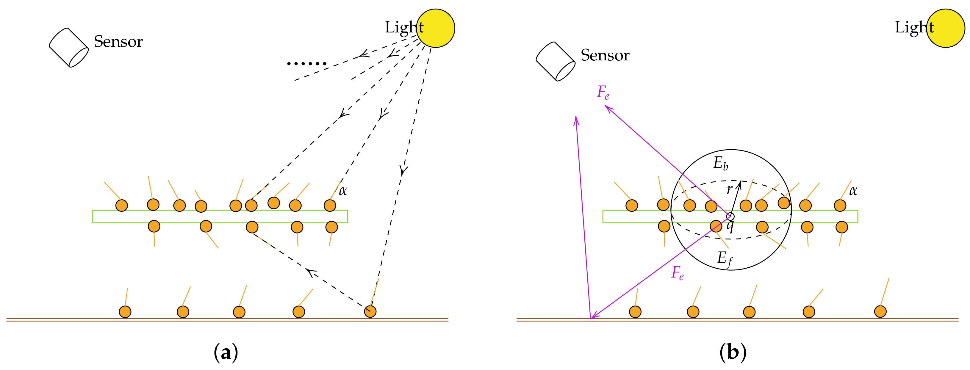
Figure 1. Schematic diagrams of the two steps of the proposed model. (a) In the first step, the point representation of the radiation is built through photon tracing, where photons with weight α are emitted from light sources and recorded upon interacting with surfaces within the scene. (b) In the second step, the routine solutions for the radiation transfer problem are adopted to solve the light transport equation, given the emitted fluorescence F e . The total SIF detected by a sensor can be divided into the direct emission from leaves and the portion that is scattered. The flux contributed by α measures the amount of light that hits a surface over a finite area (represented by the area of a circle at q with radius r here) from all directions. The irradiance E b / f integrates the light arriving at a single point q over the whole hemisphere on the backward or the forward side.
Remotesensing 16 03783 g001
Figure 2. Generated abstract scenes representing (a) homogeneous canopy (S2) and (b) row canopy (S3), respectively.
Remotesensing 16 03783 g002
Figure 3. The components’ spectra of the abstract scenes.
Remotesensing 16 03783 g003
Figure 4. Soybean leaf reflectance and transmittance spectra measured in the field.
Remotesensing 16 03783 g004
Figure 5. The components’ measured spectra of the corn scene.
Remotesensing 16 03783 g005
Figure 6. The simulated corn canopy based on the in situ measured data.
Remotesensing 16 03783 g006
Figure 7. The spectra comparisons of the total SIF (F), the emission part (Fem), and the scattering part (Fsc) in the nadir or hotspot direction for two homogeneous canopies simulated by the proposed model (dashed line) and the SCOPE model (solid line). (a) LAI = 0.9, nadir; (b) LAI = 2.1, nadir; (c) LAI = 0.9, hotspot; and (d) LAI = 2.1, hotspot.
Remotesensing 16 03783 g007
Figure 8. Polar plots of fluorescence generated by the proposed model (left panels: a,d,g) and the SCOPE model (middle panels: b,e,h), as well as their differences (right panels: c,f,i), including the total SIF at 685 nm (a,b), the total SIF at 740 nm (d,e), and the scattering part at 740 nm (g,h) for the homogeneous LAI = 2.1 scene. The sun zenith angle is at 30°, and the sun azimuth angle is at 140°.
Remotesensing 16 03783 g008
Figure 9. The angular distributions of the total SIF at 685 nm (F685) and 740 nm (F740), along with its emission part at 740 nm (Fem740) and scattering part (Fsc740) along the solar principal plane are simulated for two homogeneous canopies. These distributions are represented by a dashed line for the proposed model and a solid line for the SCOPE model. Negative-view zenith angles denote the forward direction, while positive-view zenith angles represent the backward direction. (a) LAI = 0.9; (b) LAI = 2.1.
Remotesensing 16 03783 g009
Figure 10. The SIF spectra for the soybean, reconstructed from measured data, along with simulation by the proposed model.
Remotesensing 16 03783 g010
Figure 11. The SIF distributions of the row scene (solid line) and the homogeneous scene (dashed line) simulated using the proposed model. The total SIF, the emission part, and the scattering part are denoted by F, Fem, and Fsc, respectively. (a) The spectra in the nadir direction. (b) The angular distributions along the PP at 685 nm and 740 nm. Negative-view zenith angles denote the forward direction, while positive-view zenith angles represent the backward direction.
Remotesensing 16 03783 g011
Figure 12. Polar plots of fluorescence simulated by the the proposed model model for the row scene (left panels) and the homogeneous LAI = 2.1 scene (right panels): the total SIF at 685 nm (a,b) and 740 nm (c,d), and the scattering part at 740 nm (e,f).
Remotesensing 16 03783 g012
Figure 13. Subplots illustrating the effects of spatial resolution aggregation (shown in the captions of the subplots) overlaid onto the simulated image of the row scene at 740 nm. (a) The original SIF image. (be) Different levels of aggregation in simulated images.
Remotesensing 16 03783 g013
Figure 14. Close-up of the natural color image of the row scene in the nadir view.
Remotesensing 16 03783 g014
Figure 15. Examples of SIF imaging. (a) A natural color image of the realistic corn scene. (b) The SIF image of the realistic corn scene at 685 nm with the layout of the samples (markers). Several samples are taken as examples to show the SIF imaging data. (c) The SIF spectra of the samples.
Remotesensing 16 03783 g015
Figure 16. An ideal diffuse reflectance target is attached to the sample. (a) Sample (3). (b) Sample (4).
Remotesensing 16 03783 g016
Figure 17. Examples of simulated SIF images at 685 nm at 10:30 under different light conditions of the realistic corn scene. (a) SIF image under a clear sky. (b) SIF image on a slightly hazy day. (c) The SIF spectra of the samples.
Remotesensing 16 03783 g017
Figure 18. The diurnal variations of the PAR and the SIF at 685 nm.
Remotesensing 16 03783 g018
Figure 19. The SIF versus the PAR in a day.
Remotesensing 16 03783 g019
Figure 20. Examples of the diurnal variations of the SIF at 685 nm. (a) The layout of the samples (markers) in the realistic corn scene. The samples are taken as examples to show the diurnal variations of the SIF. (b) The diurnal variations of the SIF at 685 nm.
Remotesensing 16 03783 g020
Figure 21. Examples of SIF images at 685 nm (every 1 h from 10:00 to 15:00) from the simulation of the diurnal variation of the SIF of the realistic corn scene.
Remotesensing 16 03783 g021
Table 1. Structural statistical parameters of the generated abstract scenes.
Scene IndexLeaf Area IndexAverage Leaf Angle/Standard Deviation/DegreesCanopy Height/cm
S10.954/2340
S22.154/23140
S32.154/23140
Table 2. The leaf parameters for Fluspect.
ParameterUnitDescriptionValue
N-Leaf thickness parameter1.5
Cabμg cm−2Chlorophyll AB content40
Ccaμg cm−2Carotenoid content10
CwcmLeaf water equivalent layer0.009
Cdmμg cm−2Dry matter content0.012
fqe-Fluorescence quantum yield efficiency at photosystem level0.01
Table 3. Correlation statistics between the proposed model and the SCOPE model for two scenes.
F 685 nm F 740 nm Fem 740 nm Fsc 740 nm
Scene R 2 RMSE R 2 RMSE R 2 RMSE R 2 RMSE
LAI = 0.90.98880.026 0.98760.031 0.98990.070 0.99570.056
LAI = 2.10.99390.021 0.98050.034 0.99290.059 0.99060.049
Disclaimer/Publisher’s Note: The statements, opinions and data contained in all publications are solely those of the individual author(s) and contributor(s) and not of MDPI and/or the editor(s). MDPI and/or the editor(s) disclaim responsibility for any injury to people or property resulting from any ideas, methods, instructions or products referred to in the content.