Article

Fast Hyperspectral Image Classification with Strong Noise Robustness Based on Minimum Noise Fraction

1
Unmanned System Research Institute, National Key Laboratory of Unmanned Aerial Vehicle Technology, Integrated Research and Development Platform of Unmanned Aerial Vehicle Technology, Northwestern Polytechnical University, Xi’an 710072, China
2
School of Civil Aviation, Northwestern Polytechnical University, Xi’an 710072, China
3
School of Computer Science, Northwestern Polytechnical University, Xi’an 710072, China
*
Author to whom correspondence should be addressed.
Remote Sens. 2024, 16(20), 3782; https://doi.org/10.3390/rs16203782
Submission received: 18 August 2024 / Revised: 2 October 2024 / Accepted: 9 October 2024 / Published: 11 October 2024

Abstract

:
A fast hyperspectral image classification algorithm with strong noise robustness is proposed in this paper, aiming at the hyperspectral image classification problems under noise interference. Based on the Fast 3D Convolutional Neural Network (Fast-3DCNN), this algorithm enables the classification model to have good tolerance for various types of noise by using a Minimum Noise Fraction (MNF) as dimensionality reduction module for hyperspectral image input data. In addition, by introducing lightweight hybrid attention modules with the spatial and the channel information, the deep features extracted by the Convolutional Neural Network are further refined, ensuring that the model has high classification accuracy. Public dataset experiments have shown that compared to traditional methods, the MNF in this algorithm reduces the dimensionality of input spectral data, preserves information with higher signal-to-noise ratio(SNR) in the spectral bands, and aggregates spectral features into class feature vectors, greatly improving the noise robustness of the model. At the same time, based on a lightweight spectral–spatial hybrid attention mechanism, combined with fewer spectral dimensions, the model effectively avoids overfitting. With less loss in model training speed, it achieved better classification accuracy in small-scale training sample experiments, fully demonstrating the good generalization ability of this algorithm.

Graphical Abstract

1. Introduction

In the 1980s, the emergence of hyperspectral imaging technology further expanded humanity’s ability to understand the world and explore the Earth. Compared to the technique of conventional remote sensing, hyperspectral imaging has a wider spectral range and higher spectral resolution, reaching 10 2  μm or even the nanometer level. The improvement of spectral resolution enables land features that were previously difficult to detect in traditional remote sensing technology to be included in the research scope. Due to the high spectral resolution and narrow spacing between bands, there are overlapping parts between adjacent bands of hyperspectral images, making every single pixel on the image be regarded as one concrete expression of a continuous spectral curve. This enables hyperspectral images to not only have the observed area’s spatial information but also have the corresponding land features’ spectral information, known as the “union of imagery and spectrum”, forming a hyperspectral rectangular data structure as shown in Figure 1. The commonly used Indian Pines and Salinas Scene hyperspectral datasets are both from the Airborne Visible/Infrared Imaging Spectrometer (AVIRIS) project of the USA [1], respectively, captured in 1992 and 2001. Based on the datasets, we visualized them in 3D cubes, as shown in the figure.
Hyperspectral remote sensing has rich spatial and spectral region information. Based on the differences in spectral curves, the corresponding features of each pixel in the image can be determined, providing convenient conditions for feature classification, discrimination, and analysis. Feature classification is a research hotspot in hyperspectral image analysis. Ground-truth classification is based on hard classification technology at the pixel level, which classifies and labels the pixels in an image according to the sample features and realizes the discriminant analysis of the ground truth. It has been widely used in energy and mineral exploration [2], environmental pollution monitoring [3], precision agriculture support [4], geological hazard assessment [5], perception of Battlefield Environment, assessment of Damage Effects [6], and other fields.
The general process of hyperspectral image classification mainly includes four steps: image preprocessing, training sample selection, feature extraction, and classification discrimination. According to the different types of features involved in classification, hyperspectral image classification can be divided into spectral-feature-based classification, spatial-feature-based classification, and spectral–spatial hybrid feature-based classification. Due to the “union of imagery and spectrum” and high spectral resolution, hyperspectral images contain more ground spectral–spatial features. As deep learning and intelligent information processing technologies are developing rapidly, the classification method of spectral–spatial feature fusion has gradually become mainstream, and the classification accuracy continues to improve. However, in practical applications, it is likely that hyperspectral images can be susceptible to a variety types of noise interference [7], reducing imaging quality and posing a significant challenge to classification tasks. The noise types in hyperspectral images commonly include the following: (1) Gaussian white noise: A type of noise generated by factors such as thermal noise from electronic devices and random interference during signal transmission, whose amplitude distribution follows a Gaussian (normal) distribution. Due to its additive properties and Gaussian distribution, linear filtering methods such as Gaussian filtering, median filtering, etc., can be used for effective processing. (2) Shot noise: A special type of noise generated by the interference of light waves in a medium, mainly characterized by random fluctuations in the intensity of light at different positions in an image, making the image appear to be covered by randomly distributed small papers, hence the name shot noise. In digital image processing, the presence of shot noise can have a negative impact on the quality of the image, reducing its visibility and measurement accuracy. Shot noise usually has multiplicative characteristics, and its intensity is proportional to the signal strength. Statistically, the amplitude distribution of shot noise may be Rayleigh distribution, Gaussian distribution, or other distributions, depending on the characteristics of the imaging system. Because of its multiplicative nature, traditional linear filtering methods such as Gaussian filtering often have poor performance. In image processing, nonlinear filtering methods such as adaptive filtering, model-based denoising, wavelet transform-based denoising techniques, median filtering, mathematical morphology, wavelet transform, total variation denoising, nonlocal means filtering, etc., are usually required. (3) Salt-and-pepper noise: Mainly introduced by hardware failures, distortions, or errors during image acquisition, storage, or transmission. The main characteristic of salt-and-pepper noise is the randomized distribution of the black or the white dots in images, making the image appear to be sprinkled with pepper grains (black dots) and salt grains (white dots). The intensity of these black and white dots is usually the maximum or minimum value among all pixel data, which can seriously affect the quality and usability of the image. Common denoising techniques include median filtering, average filtering, edge preserving filtering, etc., which mainly use neighborhood information to estimate the true value of pixels contaminated by salt-and-pepper noise, thereby achieving denoising [7].
In recent years, many scholars have conducted in-depth research on hyperspectral image classification under complex noise interference backgrounds and proposed a series of effective classification methods. All the methods can be mainly categorized into the following types: (1) Classification methods based on dimension reduction. This type of method maps hyperspectral images from a high-dimensional space to a low-dimensional space through dimension reduction techniques, thereby reducing the influence of noise. The commonly used dimension reduction techniques are the Principal Component Analysis (PCA) and the Kernel Principal Component Analysis (KPCA), etc. [8]. This type of method does not directly suppress noise in the image, but instead, through PCA or KPCA transformation, the important information between the multiband images is concentrated into a number of new images named the principal component, using as few as possible, and meanwhile making these principal component images not correlated with each other, thereby reducing the total data volume (equivalent to discarding some noisy band images). However, for the informative principal component, the signal-to-noise ratio is not necessarily high. If the principal component contains a large amount of information and noise, the trained model is more likely to learn the noise rather than the information we expect it to learn, and the training effect may not be very good, so the image quality may be poor. The specific measurement method is whether the noise variance is greater than the signal variance. If it is greater than, it indicates that noise dominates and the image quality may be poor; if it is less than, it indicates that the signal dominates and the image quality may not be poor. (2) Classification methods based on mixed-pixel decomposition [9,10]. This type of method decomposes mixed pixels in hyperspectral images into multiple pure pixels through mixed-pixel decomposition techniques, thereby improving classification accuracy. Common mixed-pixel decomposition techniques include Linear Spectral Mixture Model (LSMM) [11,12] and Minimum Noise Fraction (MNF), etc. This type of method separates useful pixels and noisy pixels from a sub-pixel perspective, but it can only be used as an image preprocessing operation. To achieve high classification accuracy, it must also be combined with high-performance classifiers. (3) Classification method based on deep learning [13]. This type of method utilizes deep learning techniques to extract and classify hyperspectral images. The Convolutional Neural Networks (CNNs) [14,15,16], the Recurrent Neural Network (RNN) [17], the residual network [18], etc., are the representative deep learning models. This type of method has become the mainstream method for hyperspectral image classification, but these methods all learn and classify through data-driven high-performance models and do not specifically deal with noise. Most algorithms only focus on classification accuracy and pay less attention to algorithm speed and the proportion of training samples. (4)Noise estimation and denoising-based classification methods first estimate and denoise hyperspectral images and then classify them, effectively improving classification accuracy. Common noise estimation and denoising methods include spectral decorrelation based on superpixel segmentation, frequency domain deep denoising network (D2Net), etc. [19]. However, the noise estimation of these methods only supports single-type noise, and their robustness to different noise intensities is rarely considered. On this basis, this paper proposes a fast hyperspectral image classification method with strong noise robustness. The method is based on the Fast 3D Convolutional Neural Network algorithm (Fast-3DCNN) and achieves good tolerance for all three types of noise by using an input data dimensionality reduction module based on the MNF algorithm, which is named the Minimum Noise Fraction-based Fast 3D Convolutional Neural Network (MNF-Fast-3DCNN). Meanwhile, by introducing a lightweight convolutional attention module with hybrid channel-attention and spatial-attention modules, the extracted deep features are further refined. Compared with traditional methods, the model training speed is faster, and better classification accuracy is achieved in the case of a lower training sample ratio.
This paper’s sections are sequentially organized as follows: the principle of the Fast-3DCNN algorithm is briefly summarized in Section 2. The proposed method of the MNF-Fast-3DCNN algorithm framework, including the design of the MNF module and the mixed convolutional attention module, are detailed introduced in Section 3. In Section 4, two open datasets are applied to experimentally test and analyze the algorithm’s effectiveness from the following aspects in detail: classification accuracy, noise robustness and speed. Ultimately, a conclusion will be drawn in Section 5 with future work arrangements.

2. Principle of Fast-3DCNN Algorithm

2.1. Basic Principles of Three-Dimensional Convolutional Neural Network (3DCNN)

The common Convolutional Neural Networks are usually two-dimensional Convolutional Neural Networks. Compared with them, the difference of three-dimensional Convolutional Neural Networks is that their input data, convolution kernels, and downsampling operations are all three-dimensional.
(1)
The input data for a 3D Convolutional Neural Network is three-dimensional and suitable for the rectangular data mode of hyperspectral images.
(2)
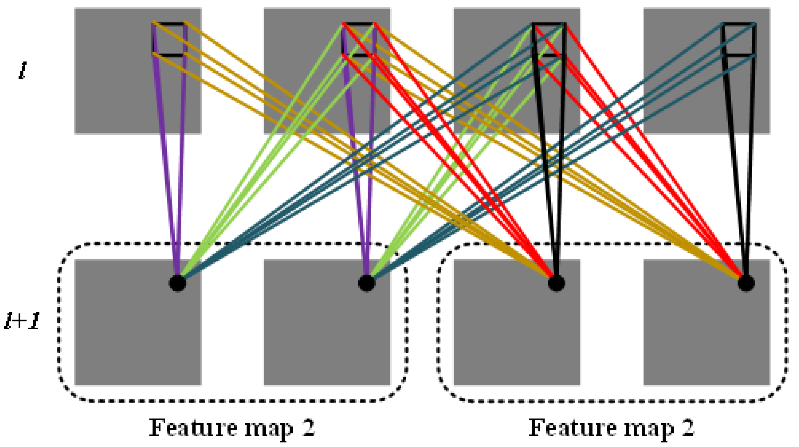
In 3DCNN, the convolutional kernels are three-dimensional, so the convolution operations are also three-dimensional. As shown in Figure 2, the third dimension of the data in the layer l is four, and there are in total two convolutional kernels, and the third dimension of each convolutional kernel is three. Furthermore, the layer l + 1 obtains two feature maps with a third dimension of two, and the lines of different colors in the diagram represent different values.
(3)
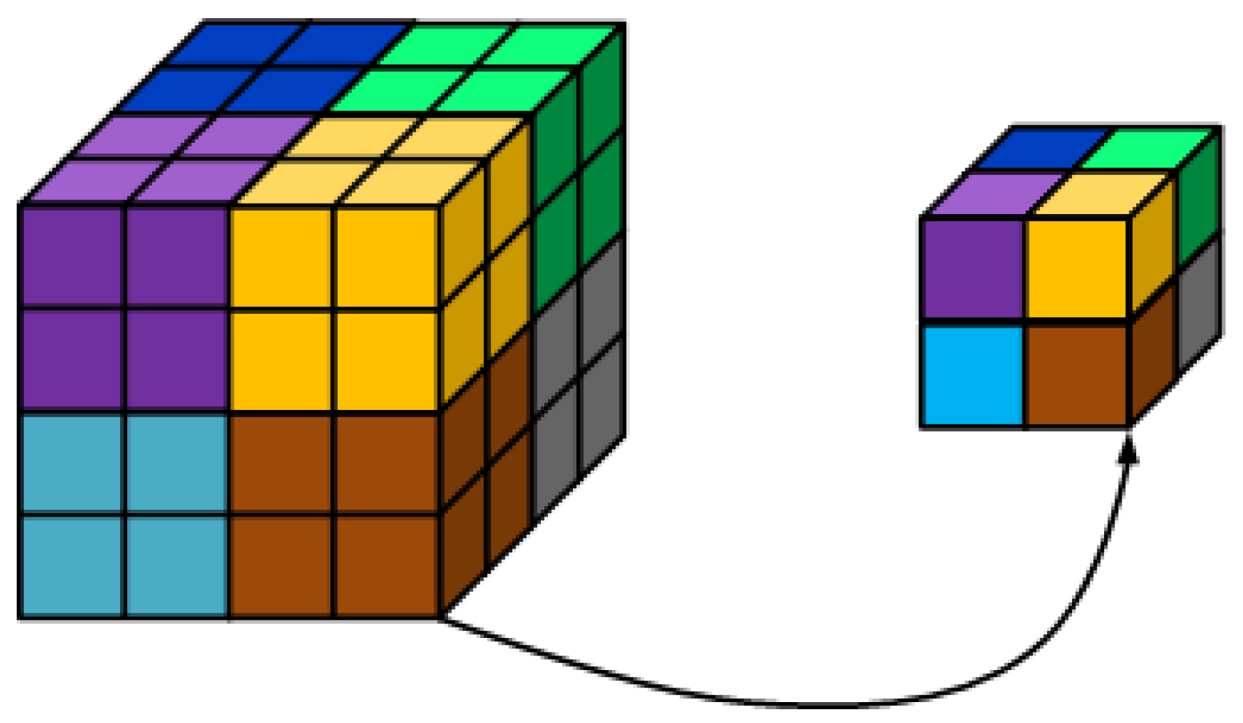
As shown in Figure 3, the 3D downsampling operation downsamples a 4 × 4 × 4 cube into a 2 × 2 × 2 cube, with a sampling interval of 2 × 2 × 2 .

2.2. Spectral–Space Joint Classification Algorithm Based on 3DCNN

The spectral–spatial hybrid classification of HSI that uses a 3DCNN will directly select a square space in the neighborhood around the target pixel in the HSI, and these cubic data are used as input for training the three-dimensional Convolutional Neural Network to obtain classification results. Figure 4 shows the schematic diagram of the classification algorithm. The number of convolutional and downsampling layers has a significant impact on the training time and overall performance of the model. Usually, increasing the number of convolutional layers improves the model’s performance, but it also increases training time and complexity. The downsampling layers can help control computational load and training time, but too many downsampling layers may lead to the loss of important information. So, finding the appropriate combination of layer numbers and network architecture usually requires experimentation to determine the best configuration. By borrowing from the algorithm in reference [20] and extensive experiments, we determined the number of convolutional and downsampling layers and the network structure in Figure 4.
There are three shortcomings in directly using 3DCNN to extract features and classify hyperspectral image data:
(1)
The network structure is too complex and requires too many training parameters. For the Indian Pines dataset, a total of three convolutional layers and three downsampling layers were used in reference [15], and the feature maps of each layer were 128, 192, and 256, respectively. It can be seen that the network is too complex and requires too many training parameters.
(2)
Often, too many iterations are required during training, resulting in slow convergence speed of the network. The required iteration number in the network in reference [15] is 400, and the training phase takes approximately 30 min.
(3)
Some methods do not take the characteristics of each band in hyperspectral images into account and only use the raw data of hyperspectral images as input to train the network. In reference [15], the 3DCNN is trained using only the raw data directly as the input. However, in hyperspectral data, the similarity between different bands is relatively high, which is often the main reason for the low classification accuracy.

2.3. Principle of Fast-3DCNN

A new fast 3D Convolutional Neural Network method was proposed in reference [17] for hyperspectral ground-truth classification problems. In this method, these HSI data cubes will be firstly separated into many mini overlapped 3D patches through domain extraction. Then, these patches are processed using 3D kernel functions to generate 3D feature maps, which preserve the union of spatial and spectral information during the process of feature learning. This process focuses on preserving the bands that have important discriminative information for HSI classification. As a preprocessing method, several methods can be used to reduce the number of bands in HSI data, such as the standard Principal Component Analysis (PCA), the incremental PCA (iPCA), the Independent Component Analysis (ICA), the Linear Discriminant Analysis (LDA), and the Non-negative Matrix Factorization (NMF), etc. As a result, the model only needs to learn the important wavelengths in the HSI cube. Then, we can train a lightweight 3DCNN with fewer parameters.
Compared with other HSI classification methods based on 2D/3D CNN, the Fast-3DCNN model proposed in reference [21] has fewer parameters and faster training speed than other neural network algorithms. This article is based on Fast-3DCNN and uses an input data dimensionality reduction module based on the MNF algorithm to achieve robustness against noise; furthermore, it is planned to add a lightweight channel–spatial attention hybrid attention module for the model to boost classification accuracy.

3. MNF-Fast-3DCNN

3.1. MNF Transform Processing of Hyperspectral Images with Noise

The PCA algorithm is extensively applied for remote sensing digital image processing, which is a multidimensional (multiband) orthogonal linear operation based on statistical characteristics. By means of PCA transformation, the important information from multiband images can be concentrated into the least amount of new principal component images necessary, and these principal component images can be made uncorrelated with each other, thereby greatly reducing the total amount of data. PCA transform is impressionable to noise, that is, for the informative principal component, the SNR is not necessarily high. The image quality can be poor when the noise variance contained in a certain informative principal component is larger than the signal variance [22]. After PCA transformation, if the variance of the noise contained in a principal component with a large amount of information is greater than the variance of the signal, the model is more likely to learn the noise rather than the information, so the image quality formed by the principal component is poor. In response to the shortcomings of PCA transformation, Green et al. proposed the Minimum Noise Fraction Rotation (MNF Rotation) [23].
The MNF tool can be used to determine the intrinsic dimensionality (i.e., number of bands) of image data, thereby separating noise from data as well as reducing computational requirements in the training processing. MNF is essentially two overlapping transformations of PCA. The first PCA transform utilizes techniques for noise isolation and realignment in data based on the estimation of noise covariance matrix, so that in the processed noise data have the minimal variance with no inter-band correlations. The second PCA transform is a common transformation applied to the noise-whitened data. The MNF transform is an orthogonal transform where the transformed components are uncorrelated and arranged in descending order of signal-to-noise ratios. After MNF transformation, the noise is separated and there is no correlation between bands, so MNF is superior to PCA transformation in high noise background data [18].
Assume that each observation signal x in the hyperspectral image we obtain is represented as
x = s + n
where s is the ideal noiseless signal and n is noise, assuming that n is uncorrelated with s. Let x be the covariance matrix of the observed signal x and n be the covariance matrix of the noise n. Suppose the matrix F is the albino matrix of n , then there is
F T n F = I , F T F = Δ n 1
where Δ n is the diagonal matrix composed of eigenvalues of Σ n . In fact, F = E Δ n 1 / 2 , where the matrix E is composed of the eigenvectors of n , satisfying E T Σ n E = Δ x .
Let Σ w = F T Σ x F be the covariance matrix of the observed data after adjusting for noise (albino), and perform principal component transformation on this matrix to obtain matrix G, such that
G T Σ w G = Λ w , G T G = I
where Λ w is another diagonal matrix composed of eigenvalues of Σ w and G is composed of the corresponding eigenvectors. The total transformation matrix of MNF can be obtained as
H = F G
MNF, also known as Noise-Adjusted Principal Components (NAPC), has two important properties: firstly, it proportionally expands any band of the image without changing the transformation result; the second is to transform the image vector, information separation, and additive noise components to be perpendicular to each other. Multiplicative noise can be transformed into additive noise through logarithmic transformation. After transformation, denoising can be applied to each component image or the components dominated by noise can be discarded. In MNF transformation, by separating the signal from the noise, information is more concentrated in a limited feature set, and some weak information is enhanced in denoising conversion. At the same time, in the MNF conversion process, the spectral features are aggregated into class feature vectors, and fewer spectral dimensions can effectively avoid overfitting of the neural network, which is beneficial for improving the model’s generalization ability and robustness.
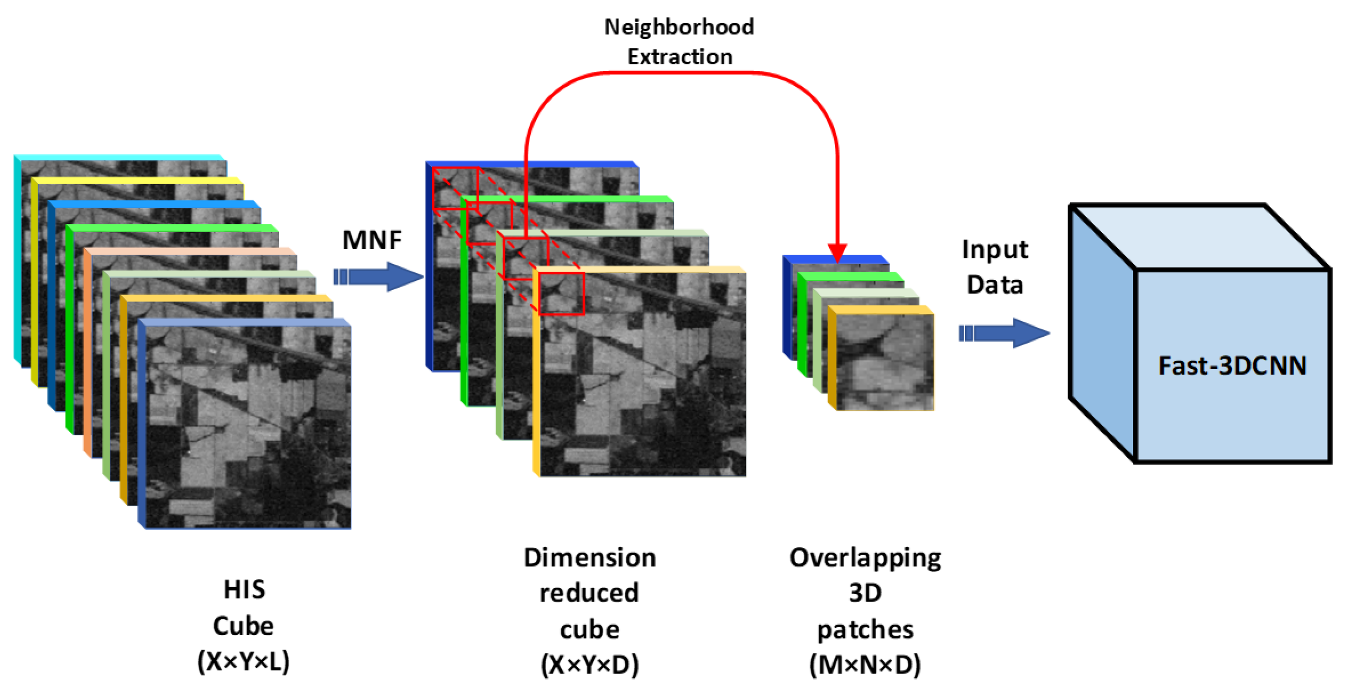
As shown in Figure 5, a series of data preprocessing steps is required before inputting hyperspectral data (with size X × Y × L, where X, Y, L, respectively, are the width, the height, and the spectral band of HSI) into the convolutional layer. Firstly, the MNF method will be used to decrease the amount of spectral bands and separate the signal from noise to make the features more concentrated; as a result, the dimension-reduced cube (with size X × Y × D, where D is the reduced dimension smaller than the original spectral band L) is obtained. Then, the HSI data with reduced spectral bands are subjected to domain extraction to obtain overlapping 3D patches (with size M*N*D, where M and N are the width and height of patches), which are then input into the Fast-3DCNN model.

3.2. Fast-3DCNN with Channel–Space Hybrid Attention Module Introduced

In this paper, the proposed Channel- and Spatial-based Convolutional Block Attention Module (CS-CBAM) is a lightweight CNN attention module that sequentially updates attention maps along the channel and the space dimensions, multiplies attention maps with input feature maps for the refinement of adaptive features, and achieves performance improvement of CNNs while maintaining low overhead [19]. The hybrid attention module consists of two parts: the channel attention module (CAM) and the spatial attention module (SAM).
The CAM: As shown in Figure 6, this module first passes the input feature through the maximum pooling and the average pooling, and it inputs the two sets of pooled data into a shared multilayer perception. After adding the two sets of data output by multiple perceptions, the final output feature of the module is obtained through an activation function. Channel attention aims to refine the channel output features of CNNs and highlight the importance of different channels in the output features.
The SAM: As described in Figure 7, the module first performs the max pooling and the average pooling on the input features along the channel axis to obtain two sets of pooled data. The two sets are then connected to form a new feature space, and a small-sized CNN is applied to the new feature space to obtain the final output features through an activation function. The spatial attention module aims to refine the spatial output features of CNNs, focusing on features at different positions in the feature space and highlighting important spatial regions.
At the same time, this paper provides answers to the question of how to arrange both the spatial and the channel attention modules. The two modules focus on important feature channels and important feature spaces in the input features, respectively. Theoretically, both parallel and serial sorting are feasible. However, the experimental results in this paper show that serial sorting is more effective than parallel sorting, and the channel-first order performs better than the spatial-first order [19].

3.3. MNF-Fast-3DCNN Network Structure

The MNF-Fast-3DCNN model’s main structure is described in Figure 8. After the input data of the model are extracted by multiple lightweight convolutional layers, the refinement of the channel output features is firstly executed with the channel attention module. Then, the same operation is executed for the spatial output features with the spatial attention module. The final output features are unfolded by the flatten function in PyTorch and put into the fully connected layer for classification, outputting the ultimate ground truth classification result.
The MNF-Fast-3DCNN model’s structure and parameters are detailed in Table 1. The first column of Table 1 shows the module types of each layer in the model. The first four layers are 3D convolutional layers, the fifth layer is a channel attention module, the sixth layer is a spatial attention module, and the seventh layer is a Flatten layer, which can receive multidimensional input data (such as two-dimensional or three-dimensional tensors) and convert them into one-dimensional tensors. The eighth to twelfth layers are alternating Linear and Dropout layers, respectively. The Linear layer is usually referred to as a fully connected layer, and its main function is to perform linear transformation on input data, that is, to perform matrix multiplication and bias operations. The Dropout layer randomly discards a portion of the activation values of neurons, mainly to prevent overfitting and improve the generalization ability of neural network models. The second column of Table 1 shows the shape of the output tensor for each layer module. The first six rows are all four-dimensional tensors, with the first dimension representing the number of channels. The second dimension represents the tensor height, which in this article’s hyperspectral image classification application represents the height of the feature map generated after the convolution operation. The third dimension represents the tensor width, which is the width of the feature map. The fourth dimension represents the tensor depth, which in this article’s hyperspectral image classification application represents the depth of feature maps generated after convolution operations. Lines 7 to 12 are one-dimensional tensors, representing the length of the tensor, where the tensor length no. of the last Linear layer is the number of categories for the classification task. The third column of Table 1 shows the result of parameter calculation, which is obtained by the following calculation method: assume the size of the convolution kernel is K × K × C i n , where K is the size in the spatial dimension (assuming the size is the same in both spatial dimensions) and C i n is the number of input feature maps. Each convolution kernel contains K × K × C i n weights plus a bias term, so the number of parameters for each convolution kernel is K × K × C i n + 1 . However, in practical calculations, the bias term is usually not considered as a parameter for each convolution kernel but rather shared by each output feature map. Therefore, the total number of parameters should be K × K × C i n × C o u t + C o u t , where C o u t is the number of output feature maps.
The setting of parameters in our model first continues using the parameter settings of Fast-3DCNN. From the table, it can be seen that the convolution kernel size used in the MNF-Fast-3DCNN model is smaller than the sizes in the 3DCNN and MS3D-CNN models. Smaller convolution kernels have the benefits of reducing the number of parameters and computational complexity, enhancing nonlinearity, and improving model flexibility and generalization ability, and they are more suitable for 3D hyperspectral image data cubes. It also can be seen that this model has 997,166 training parameters, which is 280, or slightly higher, than the 994,166 parameters of the Fast-3DCNN algorithm. That’s because we introduce the CBAM module after the convolution kernel, which only slightly increases the number of parameters in our model compared to Fast-3DCNN but can achieve significant accuracy improvement.

4. Experimental Verification and Results Analysis

In this section, two public datasets of HSI are used to compare different algorithms’ performance, namely, the Indian Pines (IP) and Salinas Scene (SA) datasets, and three typical indicators, including the Average Accuracy (AA), the Overall Accuracy (OA), and the Kappa coefficient, are introduced to evaluate the different algorithms’ classification accuracy and robustness with different hyperspectral datasets.
The IP dataset is observed by the AVIRIS sensors over the testing site of Indian Pines in northwest Indiana. The image consists of 145 × 145 pixels and 224 bands of spectral reflectance, with a 400–2500 nm wavelength range and good spatial resolution. By removing the reflection bands that cover the region of water absorption, the total number of reflection bands was reduced to 200, and the dataset consists of 16 types of land features. The SA dataset comprises imaging from the site at Salinas Valley of California, USA, with an AVIRIS and a spatial resolution of 3.7 m. The image has 512 × 217 pixels and 224 bands of spectral channels. The dataset also discards 20 regions, with 200 spectral channels available for the land cover classification. The dataset includes 16 types of land features.
In order to compare the classification accuracy of each algorithm in a noiseless environment, we conducted three sets of experiments, randomly dividing the original IP datasets with three different ratios: for the first one, 5%, 5%, and 90% were used as the training set, validation set, and test set, respectively. For the second, 10%, 10%, and 80% were the training set, validation set, and test set, respectively. For the third, 15%, 15%, and 70% were the training set, validation set, and test set, respectively. In the robustness comparison experiment of algorithms in noisy environments, we used the two publicly available hyperspectral datasets mentioned above as the original datasets and added different types of noises. The five noises added in this article are based on the three most common and typical noises found in hyperspectral images: spot noise, Gaussian white noise (GWN), and salt-and-pepper noise. These three were mixed with each other in different proportions and different intensities, and the combined noise of these five different intensities and types could better simulate the actual situation of hyperspectral remote sensing imaging, thus verifying the actual performance of our model.
We selected 5% of the IP dataset randomly as the training set, 5% as the validation set, and 90% as the testing set, and added five different intensities and types of noise to it using the above method, as follows:
(1)
GWN ( σ n = 100 ).
(2)
GWN ( σ n = 200 ).
(3)
GWN ( σ n = 300 ).
(4)
GWN ( σ n = 100 ) and shot noise.
(5)
GWN ( σ n = 100 ), shot noise and salt-and-pepper noise ( α = 0.05).
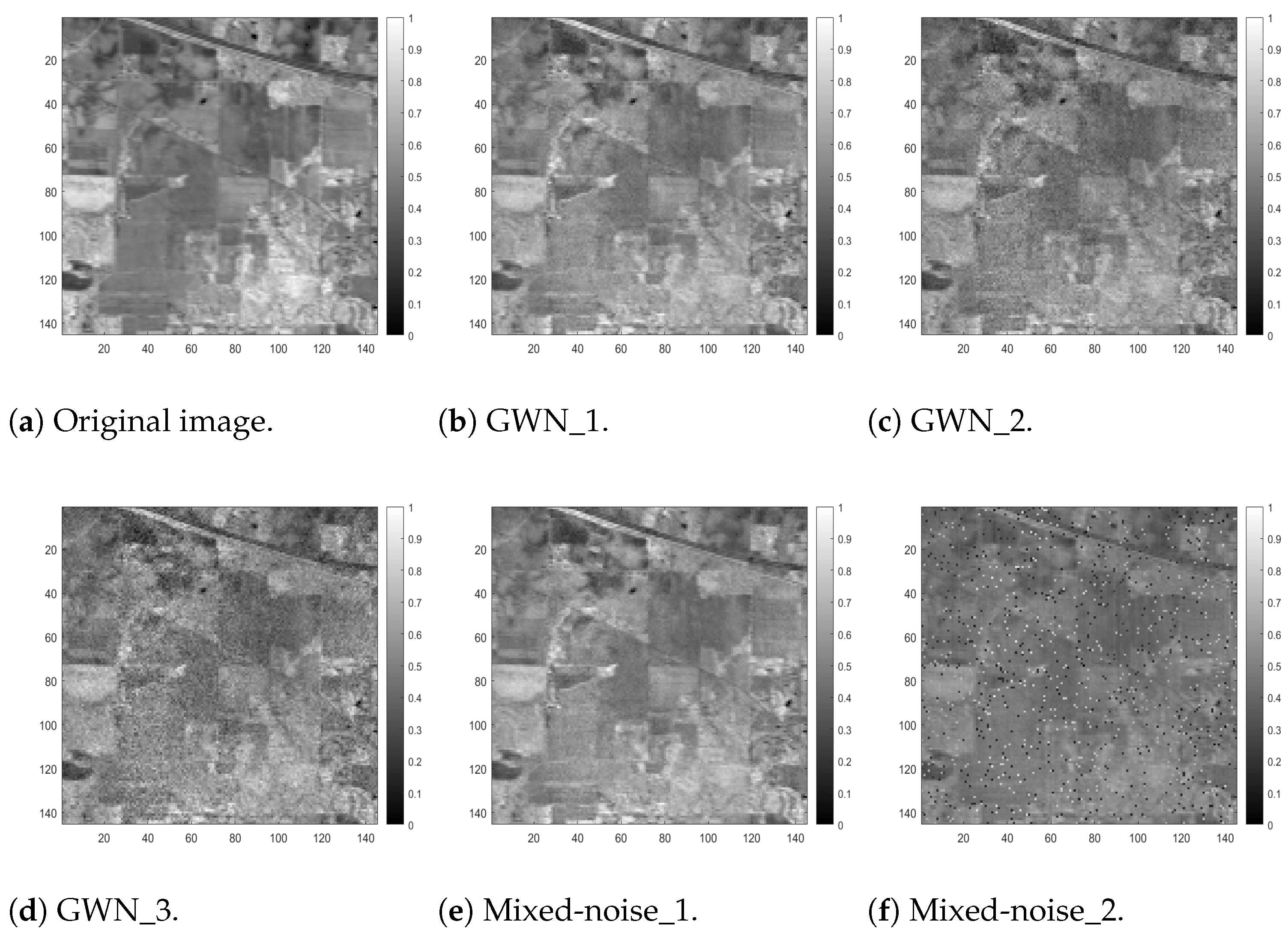
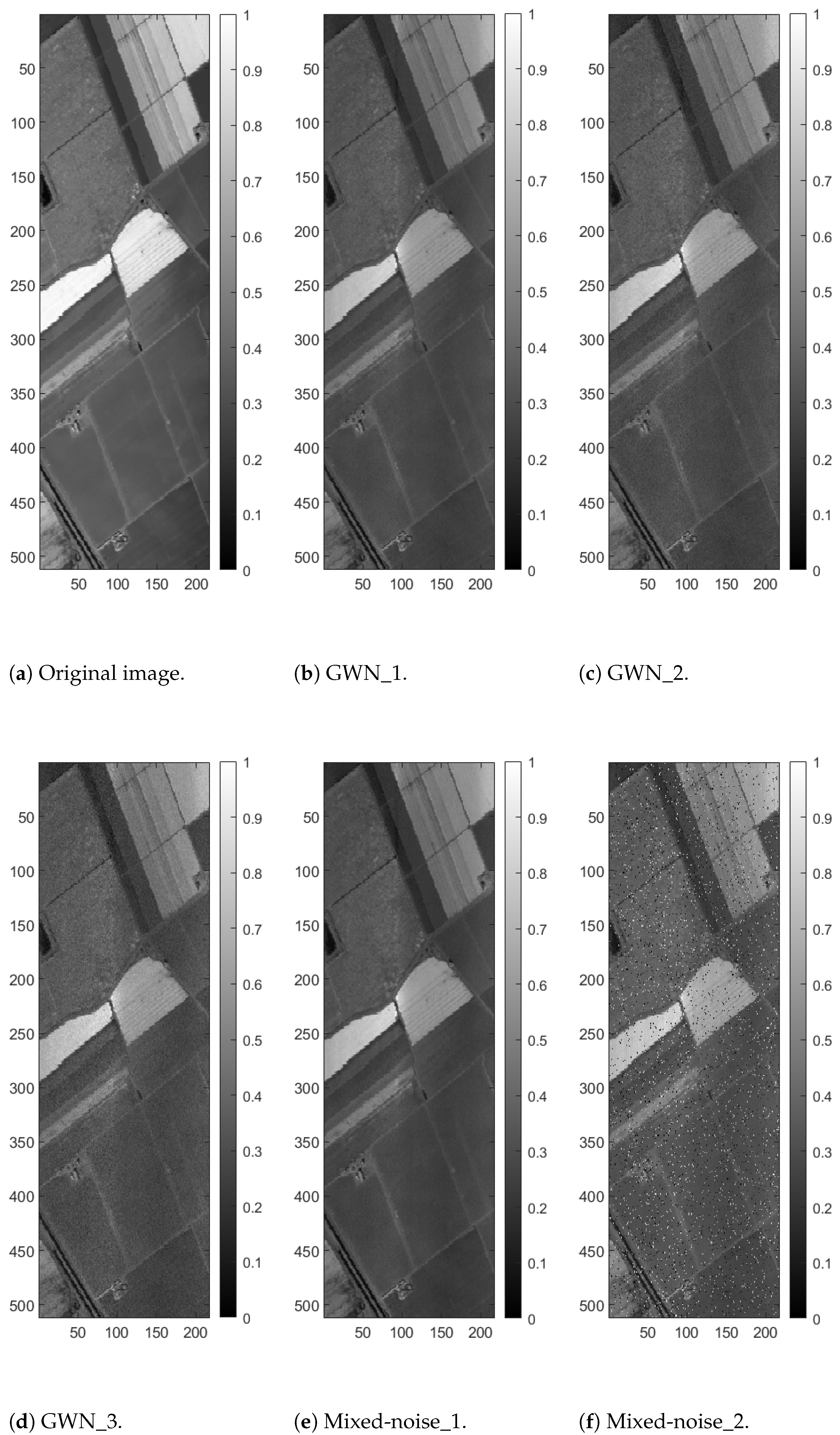
Finally, five noisy IP datasets were formed under different noise backgrounds. Figure 9 shows the noise-adding effect of the hyperspectral slice image (spectral band no. 50).
Due to the large sample size in the SA dataset and the large number of pixels in each category of land cover, in order to demonstrate the superiority of MNF-Fast-3DCNN in small-scale training sets, 1% was randomly selected as the training set, 1% as the validation set, and 98% as the testing set. The same five types of noise as the IP dataset were also added to form five SA datasets under different noise backgrounds.Finally, five noisy IP datasets were formed under different noise backgrounds. Figure 10 shows the noise-adding effect of the hyperspectral slice image (spectral band no. 50).
In order to guarantee the reliability of the comparative experiments of various algorithms during the experiment, after continuous testing and adjustment, we set each algorithm’s batch size uniformly to 64. The maximum number of epochs for the experiment was set to 200, and an early stopping strategy was set, which means that the training was stopped when the model accuracy did not improve after more than 50 epochs. All experiments were repeated 10 times.
The spectral bands’ number retained after processing the HSI cube will have a certain influence on the model classification results. In this experiment, the number of spectral bands was uniformly retained at 20 after processing, whether using PCA or MNF methods.
The Adam optimizer was introduced in the training process of the proposed network model, with an initial learning rate of 0.001 and with a learning rate decay of 1 × 10⁻⁶ in experimentation. For the Fast-3DCNN algorithm and the MNF-Fast-3DCNN proposed in this paper, the domain data extraction window size (window size) of both was uniformly set to 11 × 11 , and the rest of the algorithms were set with reference to the optimal solution given in the original paper.

4.1. Noise Robustness Experiments

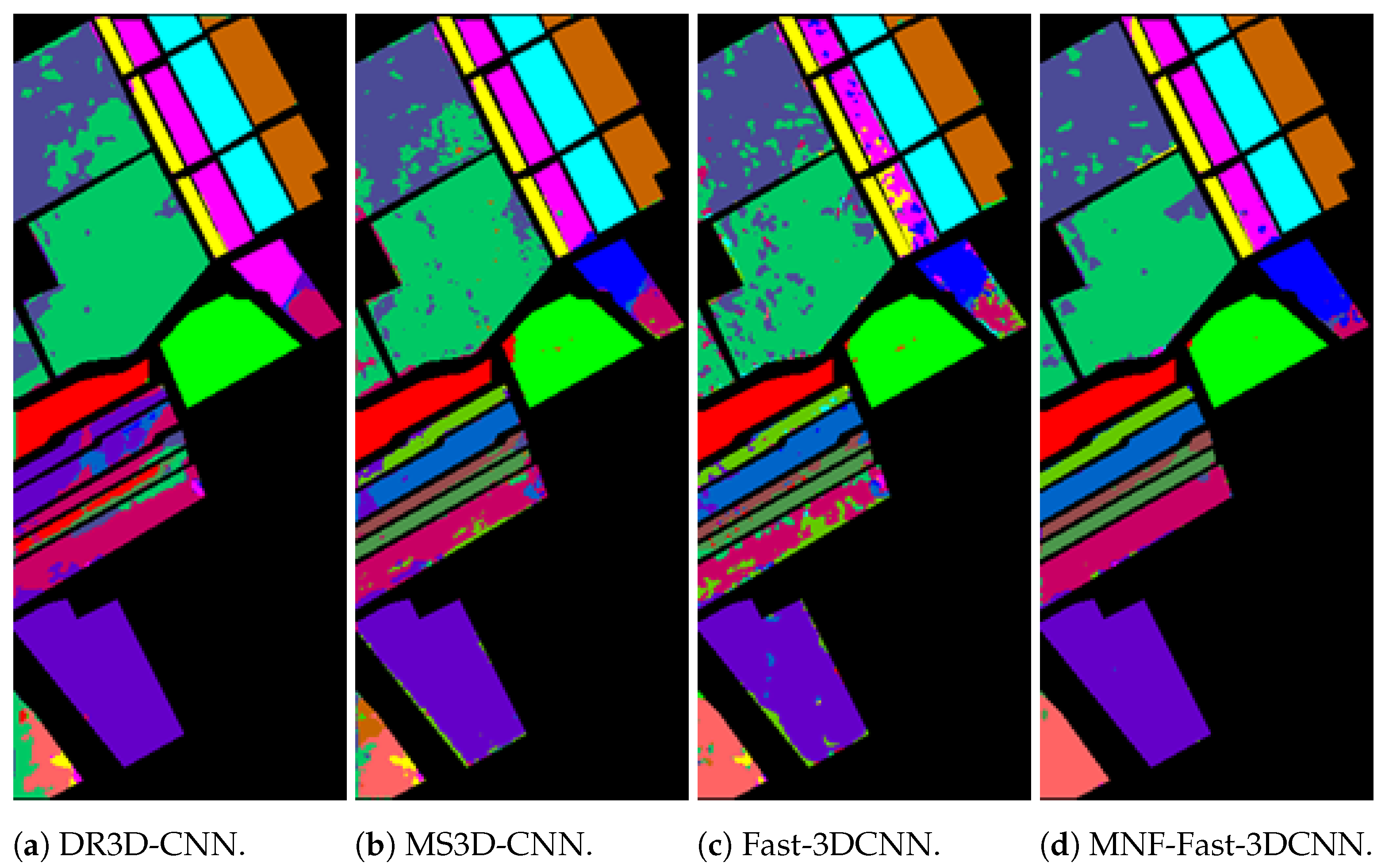
This section focuses on the key experiment of this paper, which is the robustness experiment of the algorithm under different types and intensities of noise. In this experiment, we chose DR3D-CNN [24], MS3D-CNN [25], and Fast-3DCNN [21] to be compared with the algorithm proposed in this paper. Each algorithm was tested ten times on various noisy datasets, and the results were taken as Overall Accuracy ± Standard Deviation (STD). The results on the IP dataset and the SA dataset are, respectively, shown in Table 2 and Table 3. Prediction outputs of various algorithms on IP datasets and SA datasets with GWN ( σ n = 100 ) added are, respectively, shown in Figure 11 and Figure 12.
From the table, it can be seen that our model outperforms other comparative algorithms from OA, AA, and Kappa metrics under five different noise datasets of IP and SA. Among them, the MNF-Fast-3DCNN algorithm has an average improvement of 10 percentage points in all metrics under the IP dataset and an average improvement of 7 percentage points under the SA dataset compared to Fast-3DCNN. It can be concluded that the MNF-Fast-3DCNN model proposed in this paper has strong robustness and significant advantages in various types and intensities of noise.
The experimental results show that the MNF-Fast-3DCNN algorithm has higher tolerance to various kinds of noise, due to the MNF method’s effective noise suppression performance, which can reduce the interference of noise in the model training process. The results also show that the proposed method has better classification accuracy and general applicability in the case of a small-proportion training set, as shown in Table 2 and Table 3; the method has higher classification accuracy, respectively, from the tests with 5% training samples of the IP dataset and with 1% training samples of the SA dataset.

4.2. Classification Accuracy Experiments

Then we conducted algorithm classification accuracy experiments on a small-scale training set. The algorithms are also the DR3D-CNN [24], MS3D-CNN [25], and Fast-3DCNN [21]. Table 4 shows the result of the accuracy experiments.
As can be seen from the effects, our algorithm has an improvement of over 1.5 percentage points in all indicators except for the AA coefficient, which is slightly lower than MS3D-CNN on the 5% training set. Specifically, compared to the Fast-3DCNN algorithm, the OA on the 5% training set improved by 5.7 percentage points, AA improved by 5.24 percentage points, and Kappa improved by 6.52 percentage points. Under the 10% training set, OA improved by 3.47 percentage points, AA improved by 3.82 percentage points, and Kappa improved by 3.96 percentage points. Under the 15% training set, the OA coefficient increased by 1.58 percentage points, the AA coefficient increased by 2.71 percentage points, and the Kappa increased by 1.8 percentage points. It can be concluded that the accuracy of the MNF-Fast-3DCNN method is significantly better than Fast-3DCNN and other comparative algorithms by combining with the hybrid convolutional attention module, and the improvement is particularly significant with a small-scale training set.
The MNF method preserves the information with higher SNR in the spectral bands, ensuring the “purity” of the model input data. This “purity” is more important in small-scale training sets because when the training data are insufficient, the neural network is more likely to learn the noise in the training set rather than the true intrinsic mathematical relationships of the data. Meanwhile, using a lightweight Convolutional Neural Network structure significantly reduces the number of model parameters compared to other 2D/3D CNN-based neural network models, effectively avoiding overfitting problems in small-scale training sets.

4.3. Algorithms’ Speed Experiments

Besides accuracy and robustness, it is also necessary to ensure the training speed and computational cost of the algorithm. This section conducts speed experiments on the algorithms based on this. The experiments were carried out using the IP dataset with a 5% training set ratio and the SA dataset with a 1% training set ratio, with ten experiments each. The average training time per epoch of the ten experiments was taken, in milliseconds.
To ensure fairness, all algorithms in this experiment were performed on the same server, which was configured with 128 GB of memory and an NVIDIA GeForce GTX3090 GPU. The detailed software and hardware parameter versions are shown in Table 5.
From the time per epoch metric in Table 6, it is obvious that the proposed algorithm in the paper has an essential improvement during the training procedure compared to DR3D-CNN. This is mainly because our method has a simpler network structure than DR3D-CNN, uses smaller 3D convolutions, and has fewer model parameters, which can reduce the network’s training time.
Compared to Fast-3DCNN, the algorithm proposed in this paper has a slightly longer training time, mainly due to the introduction of CBAM, which requires certain training to accurately refine the features of data in channels and space. Although our algorithm has lost some speed compared to the conventional Fast-3DCNN algorithm in the training process, it is completely acceptable because the previous experimental results have proven that our proposed algorithm has significant improvement on robustness and accuracy of classification.
In summary, the proposed MNF-Fast-3DCNN algorithm significantly improves the tolerance for various types of noise while sacrificing a small amount of running time. At the same time, it has better classification accuracy and universal applicability in small-scale training sets.

5. Conclusions

Aiming at the problems of poor noise tolerance, long training time, and low classification accuracy, an algorithm named MNF-Fast-3DCNN is proposed in this paper. The experiments base on public HSI datasets have shown that the MNF operation can greatly improving the noise robustness of the model; the algorithm also achieves better classification accuracy with small-scale training samples and generalization ability than the comparative algorithms. In the field of fast and robust hyperspectral image classification based on 3DCNN, the MNF-Fast-3DCNN method can be considered a good attempt, which can achieve good balance among the algorithm robustness, the speed, and the accuracy. In future work, the algorithm could be applied to more HSI datasets to further verify its universality. On the other hand, the limitations of the 3DCNN algorithm framework could be broken, and the transplanting feasibility of the proposed method could also be verified based on the other algorithms with high speed and accuracy.

Author Contributions

Formal analysis, G.Y.; funding acquisition, H.W.; investigation, H.W.; methodology, H.W. and G.Y.; project administration, H.W.; resources, H.W.; software, H.W. and G.Y.; supervision, H.W.; validation, H.W., G.Y., J.C. and X.W.; visualization, Z.Z.; writing—original draft, H.W.; writing—review and editing, H.W., G.Y., J.C., Z.Z., X.W. and Y.X. All authors have read and agreed to the published version of the manuscript.

Funding

This work was jointly supported by the Fundamental Research Funds for the Central Universities (Grant No. G2024KY0603) and the National Key Laboratory of Unmanned Aerial Vehicle Technology in NPU (Grant No. WR202414).

Data Availability Statement

The raw data supporting the conclusions of this article will be made available by the authors on request.

Conflicts of Interest

The authors declare no conflicts of interest.

References

  1. Available online: https://www.ehu.eus/ccwintco/index.php/Hyperspectral_Remote_Sensing_Scenes (accessed on 1 January 2024).
  2. Turner, D.J.; Rivard, B.; Groat, L.A. Visible and short-wave infrared reflectance spectroscopy of selected REE-bearing silicate minerals. Am. Mineral. 2018, 103, 927–943. [Google Scholar] [CrossRef]
  3. Lechevallier, P.; Villez, K.; Felsheim, C.; Rieckermann, J. Towards non-contact pollution monitoring in sewers with hyperspectral imaging. Environ. Sci. Water Res. Technol. 2024, 10, 1160–1170. [Google Scholar] [CrossRef]
  4. Awad, M.M. Forest mapping: A comparison between hyperspectral and multispectral images and technologies. J. For. Res. 2018, 29, 1395–1405. [Google Scholar] [CrossRef]
  5. Yamazaki, F.; Kubo, K.; Tanabe, R.; Liu, W. Damage Assessment And 3d Modeling by UAV Flights after the 2016 Kumamoto, Japan Earthquake. In Proceedings of the 2017 IEEE International Geoscience and Remote Sensing Symposium (IGARSS), Fort Worth, TX, USA, 23–28 July 2017; pp. 3182–3185. [Google Scholar]
  6. Yadav, D.; Arora, M.K.; Tiwari, K.C.; Ghosh, J.K. Detection and Identification of Camouflaged Targets using Hyperspectral and LiDAR data. Def. Sci. J. 2018, 68, 540–546. [Google Scholar] [CrossRef]
  7. Zhang, Q.; Zheng, Y.; Yuan, Q.; Song, M.; Yu, H.; Xiao, Y. Hyperspectral Image Denoising: From Model-Driven, Data-Driven, to Model-Data-Driven. IEEE Trans. Neural Netw. Learn. Syst. 2023, 35, 13143–13163. [Google Scholar] [CrossRef] [PubMed]
  8. Duan, P.; Kang, X.; Li, S.; Ghamisi, P. Noise-Robust Hyperspectral Image Classification via Multi-Scale Total Variation. IEEE J. Sel. Top. Appl. Earth Obs. Remote Sens. 2019, 12, 1948–1962. [Google Scholar] [CrossRef]
  9. Sha, L.; Zhang, W.; Ma, J.; Li, Z.; Sun, R.; Qin, M. Full-spectrum Spectral Super-Resolution Method Based on LSMM. In Proceedings of the 2022 IEEE International Geoscience and Remote Sensing Symposium (IGARSS 2022), Kuala Lumpur, Malaysia, 17–22 July 2022; pp. 2390–2393. [Google Scholar] [CrossRef]
  10. Chen, G.Y.; Krzyzak, A.; Qian, S.E. Hyperspectral Imagery Denoising Using Minimum Noise Fraction and Video Non-Local Bayes Algorithms. Can. J. Remote Sens. 2022, 48, 694–701. [Google Scholar] [CrossRef]
  11. Guilfoyle, K.; Althouse, M.; Chang, C.I. A quantitative and comparative analysis of linear and nonlinear spectral mixture models using radial basis function neural networks. IEEE Trans. Geosci. Remote Sens. 2001, 39, 2314–2318. [Google Scholar] [CrossRef]
  12. Borsoi, R.; Imbiriba, T.; Bermudez, J.C.; Richard, C.; Chanussot, J.; Drumetz, L.; Tourneret, J.Y.; Zare, A.; Jutten, C. Spectral Variability in Hyperspectral Data Unmixing. IEEE Geosci. Remote Sens. Mag. 2021, 9, 223–270. [Google Scholar] [CrossRef]
  13. Meng, Z.; Li, L.; Jiao, L.; Feng, Z.; Tang, X.; Liang, M. Fully Dense Multiscale Fusion Network for Hyperspectral Image Classification. Remote Sens. 2019, 11, 2718. [Google Scholar] [CrossRef]
  14. Roy, S.K.; Krishna, G.; Dubey, S.R.; Chaudhuri, B.B. HybridSN: Exploring 3-D-2-D CNN Feature Hierarchy for Hyperspectral Image Classification. IEEE Geosci. Remote Sens. Lett. 2020, 17, 277–281. [Google Scholar] [CrossRef]
  15. Wang, Q.; Wu, B.; Zhu, P.; Li, P.; Hu, Q. ECA-Net: Efficient Channel Attention for Deep Convolutional Neural Networks. In Proceedings of the 2020 IEEE/CVF Conference on Computer Vision and Pattern Recognition (CVPR), Seattle, WA, USA, 13–19 June 2020. [Google Scholar]
  16. Islam, M.R.; Islam, M.T.; Uddin, M.P.; Ulhaq, A. Improving Hyperspectral Image Classification with Compact Multi-Branch Deep Learning. Remote Sens. 2024, 16, 2069. [Google Scholar] [CrossRef]
  17. Zhao, H.; Feng, K.; Wu, Y.; Gong, M. An Efficient Feature Extraction Network for Unsupervised Hyperspectral Change Detection. Remote Sens. 2022, 14, 4646. [Google Scholar] [CrossRef]
  18. Zhu, M.; Jiao, L.; Liu, F.; Yang, S.; Wang, J. Residual Spectral-Spatial Attention Network for Hyperspectral Image Classification. IEEE Trans. Geosci. Remote Sens. 2020, 59, 449–462. [Google Scholar] [CrossRef]
  19. Pan, E.; Ma, Y.; Mei, X.; Huang, J.; Fan, F.; Ma, J. D2Net: Deep Denoising Network in Frequency Domain for Hyperspectral Image. IEEE/CAA J. Autom. Sin. 2023, 10, 813–815. [Google Scholar] [CrossRef]
  20. Chen, Y.; Jiang, H.; Li, C.; Jia, X.; Ghamisi, P. Deep Feature Extraction and Classification of Hyperspectral Images Based on Convolutional Neural Networks. IEEE Trans. Geosci. Remote Sens. 2016, 54, 6232–6251. [Google Scholar] [CrossRef]
  21. Ahmad, M. A Fast 3D CNN for Hyperspectral Image Classification. arXiv 2020, arXiv:2004.14152. [Google Scholar]
  22. Green, A.A.; Berman, M.; Switzer, P.; Craig, M. A transformation for ordering multispectral data in terms of image quality with implications for noise removal. IEEE Trans. Geosci. Remote Sens. 1988, 26, 65–74. [Google Scholar] [CrossRef]
  23. Woo, S.; Park, J.; Lee, J.Y.; Kweon, I.S. CBAM: Convolutional Block Attention Module. arXiv 2018, arXiv:1807.06521. [Google Scholar]
  24. Chen, S.; Jin, M.; Ding, J. Hyperspectral remote sensing image classification based on dense residual three-dimensional convolutional neural network. Multimed. Tools Appl. 2021, 80, 1859–1882. [Google Scholar] [CrossRef]
  25. He, M.; Li, B.; Chen, H. Multi-scale 3D deep convolutional neural network for hyperspectral image classification. In Proceedings of the 2017 IEEE International Conference on Image Processing (ICIP), Beijing, China, 17–20 September 2017; pp. 3904–3908. [Google Scholar] [CrossRef]
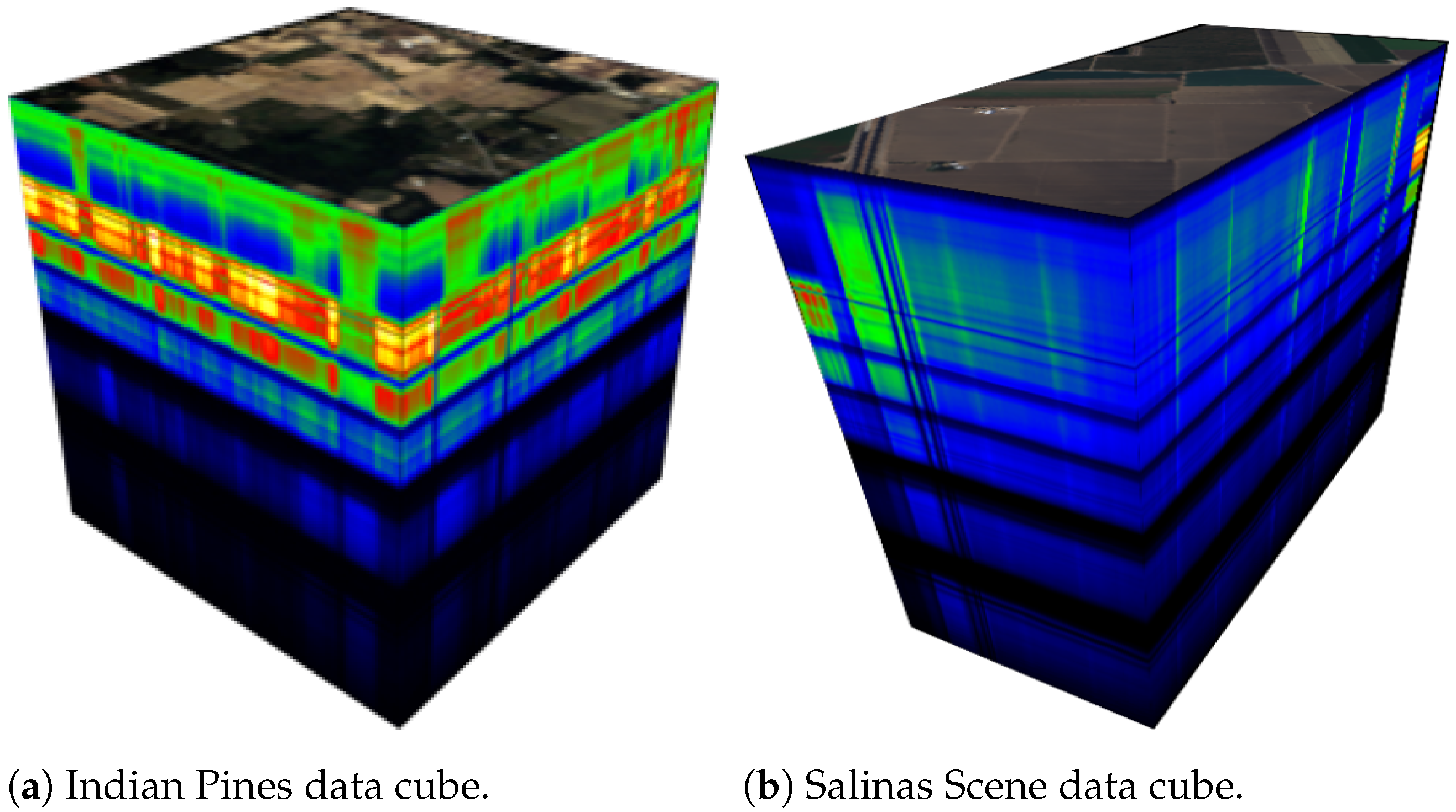
Figure 1. Typical hyperspectral image data form.
Remotesensing 16 03782 g001
Figure 2. Three-dimensional Convolutional Neural Network and convolutional operations.
Remotesensing 16 03782 g002
Figure 3. Three-dimensional downsampling.
Remotesensing 16 03782 g003
Figure 4. Spectral–space joint classification algorithm based on 3DCNN.
Remotesensing 16 03782 g004
Figure 5. Data preprocessing of MNF-Fast-3DCNN model.
Remotesensing 16 03782 g005
Figure 6. Channel attention module.
Remotesensing 16 03782 g006
Figure 7. Spatial attention module.
Remotesensing 16 03782 g007
Figure 8. MNF-Fast-3DCNN model structure diagram.
Remotesensing 16 03782 g008
Figure 9. Hyperspectral slice images (spectral band no. 50) in IP dataset with different noise added. Therein subfigure (a) is the Original image, subfigure (bd) are the images adding Gaussian white noise (GWN) with σ n = 100 , σ n = 200 and σ n = 300 respectively, subfigure (e) is the image adding the mixed-noise with GWN ( σ n = 100 ) and shot noise, subfigure (f) is the image adding the mixed-noise with GWN ( σ n = 100 ), shot noise and salt-and-pepper noise.
Remotesensing 16 03782 g009
Figure 10. Hyperspectral slice images (spectral band no. 50) in SA dataset with different noise added. Therein subfigure (a) is the Original image, subfigure (bd) are the images adding Gaussian white noise (GWN) with σ n = 100 , σ n = 200 and σ n = 300 respectively, subfigure (e) is the image adding the mixed-noise with GWN ( σ n = 100 ) and shot noise, subfigure (f) is the image adding the mixed-noise with GWN ( σ n = 100 ), shot noise and salt-and-pepper noise.
Remotesensing 16 03782 g010
Figure 11. Prediction outputs of various algorithms on IP datasets with GWN ( σ n = 100 ) added.
Remotesensing 16 03782 g011
Figure 12. Prediction outputs of various algorithms on SA datasets with GWN ( σ n = 100 ) added.
Remotesensing 16 03782 g012
Table 1. Parameters of MNF-Fast-3DCNN model with input shape (1,11,11,20) on IP dataset.
Layer (Type)Output ShapeNo. of Parameters
Convolutional3D_1 (Conv3D)(8,9,9,14)512
Convolutional3D_2 (Conv3D)(16,7,7,10)5776
Convolutional3D_3 (Conv3D)(32,5,5,8)13,856
Convolutional3D_4 (Conv3D)(64,3,3,6)55,360
Channel attention module(64,3,3,6)1024
Spatial attention module(64,3,3,6)686
Flatten_1 (Flatten)(3456)0
Linear_1 (Linear)(256)884,992
Dropout_1 (Dropout)(256)0
Linear_2 (Linear)(128)32,896
Dropout_2 (Dropout)(128)0
Linear_3 (Linear)(No. of Classes)2064
In total 997,166 trainable parameters are required.
Table 2. Algorithm comparison on five different noise datasets of IP (the optimal results are bolded, 5% training samples).
Different NoisesIndexDR3D-CNNMS3D-CNNFast-3DCNNMNF-Fast-3DCNN
(without CBAM)
MNF-Fast-3DCNN
OA0.653 ± 0.0350.765 ± 0.0160.797 ± 0.0150.890 ± 0.0180.900 ± 0.009
GWN ( σ n = 100 )AA0.408 ± 0.0450.619 ± 0.0230.698 ± 0.0210.818 ± 0.0350.841 ± 0.009
Kappa0.588 ± 0.0440.729 ± 0.0190.768 ± 0.0170.874 ± 0.0210.886 ± 0.010
OA0.622 ± 0.0200.732 ± 0.0160.777 ± 0.0120.865 ± 0.0090.876 ± 0.008
GWN ( σ n = 200 )AA0.384 ± 0.0330.581 ± 0.0250.678 ± 0.0240.797 ± 0.0310.806 ± 0.019
Kappa0.549 ± 0.0260.689 ± 0.0190.745 ± 0.0130.846 ± 0.0110.858 ± 0.009
OA0.590 ± 0.0190.682 ± 0.0240.758 ± 0.0220.848 ± 0.0120.852 ± 0.014
GWN ( σ n = 300 )AA0.339 ± 0.0270.531 ± 0.0400.663 ± 0.0290.780 ± 0.0200.780 ± 0.038
Kappa0.509 ± 0.0240.631 ± 0.0280.723 ± 0.0260.826 ± 0.0140.831 ± 0.016
GWN ( σ n = 100 ), shot noiseOA0.678 ± 0.0170.762 ± 0.0140.797 ± 0.0120.888 ± 0.0170.897 ± 0.009
AA0.433 ± 0.0180.609 ± 0.0190.690 ± 0.0160.826 ± 0.0290.821 ± 0.018
Kappa0.620 ± 0.0220.725 ± 0.0160.765 ± 0.0140.872 ± 0.0190.882 ± 0.011
GWN ( σ n = 100 ), shot noise, salt and pepper ( α = 0.05 )OA0.594 ± 0.0160.686 ± 0.0090.782 ± 0.0190.834 ± 0.0140.850 ± 0.009
AA0.333 ± 0.0230.533 ± 0.0230.679 ± 0.0300.746 ± 0.0230.751 ± 0.026
Kappa0.514 ± 0.0210.636 ± 0.0120.751 ± 0.0210.810 ± 0.0160.829 ± 0.010
Table 3. Algorithm comparison on five different noise datasets of SA (the optimal results are bolded, 1% training samples).
Different NoisesIndexDR3D-CNNMS3D-CNNFast-3DCNNMNF-Fast-3DCNN
(without CBAM)
MNF-Fast-3DCNN
OA0.810 ± 0.0180.888 ± 0.0150.861 ± 0.0180.938 ± 0.0100.947 ± 0.009
GWN ( σ n = 100 )AA0.669 ± 0.0340.875 ± 0.0150.856 ± 0.0120.936 ± 0.0160.940 ± 0.014
Kappa0.786 ± 0.0210.875 ± 0.0240.846 ± 0.0190.932 ± 0.0110.941 ± 0.010
OA0.776 ± 0.0150.874 ± 0.0130.855 ± 0.0190.911 ± 0.0200.927 ± 0.012
GWN ( σ n = 200 )AA0.620 ± 0.0220.864 ± 0.0200.835 ± 0.0240.908 ± 0.0220.919 ± 0.014
Kappa0.748 ± 0.0170.859 ± 0.0140.838 ± 0.0210.901 ± 0.0220.919 ± 0.013
OA0.756 ± 0.0090.875 ± 0.0040.843 ± 0.0180.898 ± 0.0110.898 ± 0.010
GWN ( σ n = 300 )AA0.598 ± 0.0180.863 ± 0.0120.820 ± 0.0180.894 ± 0.0140.901 ± 0.015
Kappa0.724 ± 0.0110.861 ± 0.0050.825 ± 0.0200.887 ± 0.0120.886 ± 0.012
GWN ( σ n = 100 ), shot noiseOA0.806 ± 0.0140.890 ± 0.0110.870 ± 0.0160.941 ± 0.0060.950 ± 0.007
AA0.662 ± 0.0240.877 ± 0.0160.853 ± 0.0270.933 ± 0.0130.945 ± 0.008
Kappa0.782 ± 0.0170.877 ± 0.0120.855 ± 0.0180.935 ± 0.0070.944 ± 0.008
GWN ( σ n = 100 ), shot noise, salt and pepper ( α = 0.05 )OA0.701 ± 0.0160.851 ± 0.0110.828 ± 0.0230.860 ± 0.0210.873 ± 0.017
AA0.545 ± 0.0200.839 ± 0.0230.812 ± 0.0190.842 ± 0.0360.854 ± 0.029
Kappa0.661 ± 0.0190.833 ± 0.0120.808 ± 0.0250.844 ± 0.0240.858 ± 0.019
Table 4. Classification performance of different algorithms taking 5%, 10%, and 15% samples as training set with IP dataset (the optimal results are bolded).
IndexClassification Accuracy of Each Algorithm (%)
DR3D-CNNMS3D-CNNFast-3DCNNMNF-Fast-3DCNN
OA (5%)67.3282.0188.3994.09
AA (5%)45.6689.7879.9185.15
Kappa (5%)61.5279.3086.7593.27
OA (10%)71.2785.5393.3096.77
AA (10%)55.0491.0290.9394.75
Kappa (10%)66.9783.7092.3696.32
OA (15%)79.7489.7196.5998.17
AA (15%)61.9991.4493.1595.86
Kappa (15%)76.2488.3096.1197.91
Table 5. Details of experimental environment configuration.
Experimental EnvironmentHardware Parameters and Software Version
OSUbuntu-20.04
GPUNVIDIA GeForce GTX3090
Memory128 G
Programming languagePython 3.8.19
Deep learning frameworkPytorch 2.3.0
Table 6. Comparison experiments of algorithm training speed (ms).
\DR3D-CNNMS3D-CNNFast-3DCNNMNF-Fast-3DCNN
IP474.14104.6572.07102.33
SA407.8389.9563.1887.10
Disclaimer/Publisher’s Note: The statements, opinions and data contained in all publications are solely those of the individual author(s) and contributor(s) and not of MDPI and/or the editor(s). MDPI and/or the editor(s) disclaim responsibility for any injury to people or property resulting from any ideas, methods, instructions or products referred to in the content.