Abstract
Accurate, continuous, and reliable positioning is critical to achieving autonomous driving. However, in complex urban canyon environments, the vulnerability of stand-alone sensors and non-line-of-sight (NLOS) caused by high buildings, trees, and elevated structures seriously affect positioning results. To address these challenges, a sky-view image segmentation algorithm based on a fully convolutional network (FCN) is proposed for NLOS detection in global navigation satellite systems (GNSSs). Building upon this, a novel NLOS detection and mitigation algorithm (named S−NDM) uses a tightly coupled GNSS, inertial measurement units (IMUs), and a visual feature system called Sky−GVIO with the aim of achieving continuous and accurate positioning in urban canyon environments. Furthermore, the system combines single-point positioning (SPP) with real-time kinematic (RTK) methodologies to bolster its operational versatility and resilience. In urban canyon environments, the positioning performance of the S−NDM algorithm proposed in this paper is evaluated under different tightly coupled SPP−related and RTK−related models. The results exhibit that the Sky−GVIO system achieves meter-level accuracy under the SPP mode and sub-decimeter precision with RTK positioning, surpassing the performance of GNSS/INS/Vision frameworks devoid of S−NDM. Additionally, the sky-view image dataset, inclusive of training and evaluation subsets, has been made publicly accessible for scholarly exploration.
1. Introduction
Currently, the synergistic use of global navigation satellite systems (GNSSs) and inertial navigation systems (INSs) has emerged as the predominant approach to navigate complex urban environments [1,2,3]. Within the domain of GNSSs, real-time kinematic (RTK) and precise point positioning (PPP) technologies have been extensively adopted to enhance GNSS/INS integrated solutions. Comparative studies indicate that RTK/INS fusion yields a superior accuracy over PPP/INS under identical observational conditions [4]. Nonetheless, urban environments, with pervasive obstructions like edifices and arboreal coverage, introduce non-line-of-sight (NLOS) errors into GNSS signals, compromising the accuracy of integrated GNSS/INS positioning. To address the impact of NLOS on GNSS/INS systems, researchers have experimented in recent years with additional sensors to detect and suppress NLOS, including fish-eye cameras, LiDAR, and 3-dimensional (3D) maps. Since sensor information can truly reflect the environment around a vehicle, it has become a hot topic to investigate additional sensor-based NLOS detection to improve the positioning accuracy and robustness of GNSS-related systems in urban canyons.
Cameras are increasingly utilized in vehicular motion estimation due to their energy efficiency and cost benefits. As an external sensor, cameras can provide rich environmental features for vehicle motion estimation [5,6,7]. Consequently, the integration of cameras with GNSS- and micro-electro-mechanical system (MEMS)-based inertial measurement units (IMUs) is a common strategy to attain precise localization in complex urban environments. Previous research [8] has introduced a monocular model of visual–inertial navigation systems (VINSs), integrating visual inertial odometry (VIO)-derived relative poses with global positioning system (GPS) data within a unified optimization structure. In contrast to VINS-Mono, the work in [9] combines differential GNSS results with the VIO model, in which the VIO model is transformed from the local frame to the global frame, achieving meter-level positioning accuracy in complex urban environments. Advancing from VINS-Mono, the work in [10] introduced the well-known GVINS model, which performs a joint optimization of GNSS pseudorange measurements, visual features, and inertial measurements through factor graph optimization techniques. While methods based on nonlinear optimization have advantages in handling system nonlinearity, multiple iterations of optimization increase computational complexity. Therefore, some researchers have started to focus on extended Kalman filter (EKF)-based methodologies. Building on [11], a paper [12] put forth a tightly-coupled Mono/MEMS-IMU/single-frequency GNSS-RTK model employing a multi-state constraint Kalman filter (MSCKF), which attained decimeter-level positioning accuracy in urban environments.
In the above multi-sensor fusion positioning systems, the GNSS is the only subsystem that provides absolute position information. Therefore, the quality control of the GNSS raw measurements determines the overall performance of the system. This underscores the significance of NLOS signal detection and mitigation, especially in the convoluted terrains of urban environments.
In the detection and mitigation of GNSS NLOS signals, strategies are divided into hardware-centric designs and algorithmic advancements. Compared to expensive hardware improvements such as antenna design in [13,14], many researchers have focused on algorithmic improvements. These include empirical weighting models based on the elevation angle [15], signal-to-noise ratio (SNR) [16], and methods that leverage multi-source information for satellite visibility. Notably, methods augmented by external sources like LiDAR [17,18], 3D maps [19,20], and cameras [21,22] have a refined GNSS NLOS signal detection accuracy. In particular, cameras present a cost-effective alternative to the high expenses and limited scope of LiDAR and the need for continuously updated 3D map databases. Infrared cameras [23] exhibit varying results for objects at different temperatures, making it easier to distinguish between sky and non-sky areas, which is advantageous for determining a satellite’s projection location on sky-view images. However, compared to regular fish-eye cameras, infrared cameras are more costly. Furthermore, these cameras have not yet seen widespread use in consumer market products, like smartphones or vehicle-mounted cameras. Subsequently, many research works began to use sky-pointing fish-eye cameras to capture sky-view images. These images were processed using segmentation algorithms [24,25,26] to distinguish between sky and non-sky areas. Finally, the satellites received by a GNSS receiver were projected onto the sky-view images, facilitating the visualization of GNSS NLOS satellites. As seen from the results in [23,27], this approach significantly enhances the performance of SPP/INS positioning in complex urban environments. However, these traditional segmentation algorithms may not adapt well to sky-view images with varying lighting conditions. Furthermore, we have observed that the use of sky-view images for GNSS NLOS detection has not been extended to tightly coupled GNSS/INS/Vision systems. Additionally, there is an absence of comparative performance analyses of sky-view images in different GNSS positioning modes, both domestically and internationally.
We aim to extend the sky-view image-aided GNSS NLOS detection and mitigation method (named S−NDM) to the tightly coupled GNSS/INS/Vision system, thereby enhancing vehicle positioning performance in urban canyons. Here, we particularly emphasize the progression from the work of [27] through the following points: (a) Different from the previous idea of improving the region growth algorithm, we use the algorithm of a neural network to achieve segmentation of sky-view images to adapt to different lighting conditions; and (b) While the original NLOS signal processing algorithm is only used in a tightly coupled SPP/INS framework, in this paper, we extend it to a tightly coupled SPP/INS/Vision and RTK/INS/Vision framework. In addition, we evaluate the performance of the algorithm in these two frameworks and verify the practicability of the algorithm. This paper emphasizes the following primary contributions:
- Adaptive Sky-view Image Segmentation: We introduce adaptive sky-view image segmentation based on fully convolutional networks (FCNs) that can adjust to varying lighting conditions, addressing a key limitation of traditional methods;
- Integration of Sky-GNSS/INS/Vision: We propose an integrated model that combines GNSS, INS, and Vision. Meantime, we extend the S−NDM method to this model (named Sky−GVIO), enabling a comprehensive approach to vehicle positioning in challenging urban canyon environments;
- Performance Evaluation: A comprehensive evaluation of S−NDM’s performance is conducted, with a focus on its effectiveness within GNSS pseudorange and carrier-phase positioning frameworks, thereby shedding light on its applicability across different GNSS-related integration positioning techniques;
- Open-Source Sky-view Image Dataset: An open-source repository of sky-view images, including the training and testing data, is provided at https://github.com/whuwangjr/sky-view-images, accessed on 27 July 2024, contributing a valuable dataset to the research community and mitigating the lack of available resources in this field.
2. System Overview
The proposed model, Sky−GVIO, is described in this section, including sky-view image segmentation based on an FCN, the tightly coupled GNSS/INS/Vision integration system, and S−NDM, as shown in Figure 1. The tightly coupled model is a fusion of the observed values. Before the fusion, it is very important to process the original GNSS observations. We use the S−NDM algorithm to process GNSS NLOS signals. In addition, the INS mechanization is used for state prediction and the system covariance is also propagated. In the visual part, the feature extraction and tracking will be performed following [11]. Finally, we integrate the observation equations of GNSS, INS, and Vision into the MSCKF framework to obtain the navigation results.
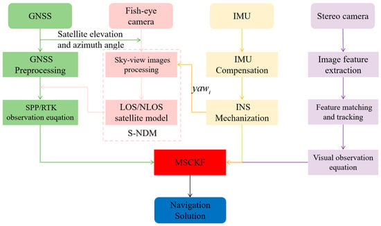
Figure 1.
The system structure of the proposed Sky-GVIO.
2.1. Sky-View Image Segmentation
Sky-view images can be significantly affected by factors such as clouds and lighting conditions, making it challenging to achieve high-precision segmentation using traditional methods based on pixels [28], categories [29], regions [30], and so on. It is well known that FCNs represent mature pixel-level semantic segmentation networks [31]. The FCN network structure primarily consists of two parts: the fully convolutional part and the deconvolution part. The fully convolutional part comprises classical CNN networks, such as VGG and ResNet, which are used for feature extraction. The deconvolution part, on the other hand, upsamples the feature maps to obtain the original-sized semantic segmentation image.
In this paper, ResNet50 [32] is chosen for downsampling, based on the advantages of its residual structure in dense semantic segmentation tasks. The residual connections in ResNet50 effectively alleviate the vanishing gradient problem in deep networks, making it easier for the model to learn rich features during training. This structure not only accelerates model convergence but also enhances feature extraction capabilities, making it particularly suitable for handling complex sky-view images. For the upsampling part, the FCN-8s architecture was adopted. FCN-8s uses transposed convolution to upsample feature maps at 8×, 16×, and 32× scales back to their original size and combines these three scaled feature maps using skip connections. This method ensures the learning of features at different scales, thereby improving the model’s performance in the sky image segmentation task. By integrating information at different scales, FCN-8s can better capture image details, thereby improving the accuracy and robustness of semantic segmentation. In summary, the combination of ResNet50 and FCN-8s allows this study to effectively address the challenges of sky-view image segmentation.
For the sky-view image segmentation task, two types of labels are required (sky region and non-sky region), so the number of channels for the sky-view image segmentation algorithm based on an FCN is two. In addition, in this study, we made 440 training datasets by ourselves. As shown in Figure 2, we built a sky-view image segmentation model based on an FCN.
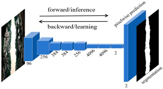
Figure 2.
The sky-view image segmentation algorithm based on FCN.
2.2. Tightly Coupled GNSS/INS/Vision Integration Model
First, this section provides a brief background on the GNSS observation model, the INS dynamic model, and the visual observation model to pave the way for homogeneous sensor fusion. In light of the aforementioned, the state model and the measurement model of the Sky−GVIO are described. Finally, NLOS detection is implemented using the segmentation results discussed in Section 2.1, and an LOS/NLOS model is established to mitigate NLOS effects.
- (1)
- GNSS Observation Model: The original pseudorange and carrier-phase observation equations in GNSS positioning are expressed as follows:where and represent the pseudorange and carrier phase, respectively. The angular symbols and refer to satellites and receivers, respectively. denotes the geometric distance between the phase centers of the receiver and satellite antennas. and represent the receiver and satellite clock offsets, respectively. The speed of light is . and refer to the ionospheric and troposphere delay, respectively. represents the carrier wavelength. represents the carrier-phase ambiguity. and represent the pseudorange noise and carrier-phase noise, respectively.
For the SPP model, Equation (1) is sufficient. However, in the case of the RTK model, it can be represented as follows:
where denotes the double-differenced (DD) operator. The DD operation is used to not only eliminate satellite orbit errors and clock errors but also to mitigate receiver clock errors as well as tropospheric and ionospheric delays, making it a powerful technique in GNSS positioning.
- (2)
- INS Dynamic Model: Considering the noisy measurement of the low-cost IMU, the Coriolis and centrifugal forces due to Earth’s rotation are ignored in the IMU formulation. The inertial measurement can be modeled [21] in the (body) frame as follows:where is the output of the IMU at time , and is the linear acceleration and angular velocity of the IMU sensor. and are the biases of the accelerometer and gyroscope at time , respectively. In addition, and are assumed to be zero-mean Gaussian-distributed with and . denotes the rotation matrix from the IMU body (b) frame to the n frame. is the gravity in the n frame.
The linearized INS dynamic model [30] can be expressed as follows:
where , , and represent the derivative of the position, velocity, and attitude errors in the (navigation) frame, respectively. “” is the cross-product. and denote the accelerometer and gyroscope bias errors, respectively. and are assumed to be zero-mean Gaussian-distributed with and [7]. Therefore, the error state vector of INS can be expressed as follows:
- (3)
- Visual Measurement Model: The core idea of the well-known MSCKF is to establish geometric constraints between multi-camera states by utilizing the same visual feature points observed by multi-cameras. Following this concept, we establish a visual model. For a visual feature point observed by a stereo camera at time , its visual observation model [33] on the normalized projection planes of the left and right cameras can be represented as follows:where the subscripts 0 and 1 represent the left and right cameras, respectively. are the pixel coordinates of the feature points on the normalized plane. is the visual measurement noise. represents the feature position in the camera (c) frame, which can be expressed as follows:where and are the rotation matrix and position of the left camera in the n frame, respectively. is the rotation matrix of the left camera to the right camera, and is the translation matrix of the left camera to the right camera, which can be accurately corrected in advance [34]. and , respectively, are the positions of the visual feature point in the n frame and left c frame. We adopted the method proposed by [35] to construct the visual reprojection error between relative camera poses, and the visual state vector was described as follows:where and , respectively, represent the rotation and position error at the time . The subscript represents the total number of camera poses (defined as rotations and translations) in the sliding window. The reprojection residual of a visual measurement can be expressed as follows:where and , respectively, represent the observed and reprojected visual measurements. is the Jacobi matrix of the camera states involved. Specific details can be obtained from [35].
- (4)
- State and Measurement Model of the Tightly Coupled GNSS/INS/Vision: This paper employs MSCKF for tightly coupled GNSS/INS/Vision integration. Based on the above introductions of different sensor models, the complete state model for the integration of tightly coupled GNSS/INS/Vision is as follows:
For both SPP and RTK positioning modes, this paper has constructed their state models separately:
where represents the double-difference carrier-phase ambiguity. In addition, the error state model of the INS and Vision have already been provided in Equations (7) and (11).
The state prediction model for the integration of tightly coupled GNSS/INS/Vision is as follows:
In Equation (16), is the continuous-time state transition matrix of INS. and are the process noise of the INS and GNSS, respectively. Based on Equation (6), the special form of can be written as follows:
where is the identity matrix.
To deal with discrete time measurement from the INS, the fourth-order Runge–Kutta [10] numerical integration of Equation (17) is used to propagate the estimated state variables. It is worth noting that only the IMU state variables are propagated; the visual and GNSS state variables are only copied. Meanwhile, we also need to propagate the covariance of the state:
where represents the discrete state transition matrix, is the continuous time state transition matrix at time (), and is the discrete time noise covariance. represents the error state covariance matrix before augmentation. represents the one-step prediction error covariance matrix from time to time .
It is worth noting that every time a new image is recorded, the state and covariance matrix will be augmented with a copy of the current camera pose estimate. The initial value of the camera pose is derived from the INS mechanization, and the covariance matrix after augmentation can be expressed as follows:
where and represent the number of variables related to the GNSS and Vision at a certain moment. When the GNSS is recorded, we only need to remove and add state variables and the corresponding covariance. is the Jacobi matrix, which has the following form:
where and are the rotation matrix and translation matrix between the camera and IMU, which are calibrated offline [36].
Based on the previous equations, the measurement equations for the integration of tightly coupled SPP/INS/Vision are formulated as follows:
where is the error of the pseudorange observation for SPP, and is the error of the visual observation in Equation (12). is the Jacobi matrix of the pseudorange error, and is the Jacobi matrix of the involved camera states in Equation (12). Then, , , and are the error state vectors of INS, SPP, and Vision, which can be found in Equations (7), (11), and (14), respectively. In the same way, and denote the pseudorange observation error noise for SPP and the visual observation error noise, respectively. In addition, and are, respectively, the actual measured pseudorange in Equation (1) and the pseudorange predicted by INS mechanization. and , respectively, represent the observed and reprojected visual measurements in Equation (12).
The measurement equations for the integration of tightly coupled RTK/INS/Vision are formulated as follows:
where and represent the observation errors of the DD pseudorange and the DD carrier phase in RTK positioning, respectively. and can be found in Equation (3). In addition, and are the DD pseudorange predicted and the DD carrier phase predicted by INS mechanization, respectively. Then and are the Jacobi matrices of the DD pseudorange error and DD carrier-phase error. is the error state vector of RTK positioning, which can be found in Equation (15). and denote the DD pseudorange observation error noise and DD carrier-phase observation error in RTK positioning.
In Equation (23), . and refer to elevation angles and the SNR of satellites, respectively. The work [37] gives the parameters of , , , and ; these are empirical values. and represent the standard deviation of the pseudorange and carrier phase, respectively, which are 0.3 m and 0.03 m in this paper. The is the scale factor, which is 10 in this paper. If the satellite’s projection is located in the sky semantic region, then a stochastic model of the satellite observations will be modeled by using Equation (24), and if not, it will be modeled by using Equation (23).
2.3. The Sky-View Image-Aided GNSS NLOS Detection and Mitigation Method (S−NDM)
For the accurate modeling of the GNSS noise covariance in the integration of tightly coupled GNSS/INS/Vision, it is essential to differentiate between LOS and NLOS satellites. Therefore, we obtain a sky-mask after performing the semantic segmentation of the sky-view images using an FCN, and subsequently, based on the projection model mentioned in [27] and the satellite information, including the elevation and azimuth angles provided by the satellite ephemeris, we ultimately identify the LOS and NLOS conditions around the GNSS receiver. Figure 3 shows the overall flow of the S−NDM algorithm. In this process, if the satellite’s projection is located in the sky region, then the satellite will be classified as an LOS satellite (represented by a blue dot), and if not, it will be classified as an NLOS satellite (represented by a red dot). Through this satellite visualization strategy, we can obtain the judgment conditions of Equations (22) and (23). This satellite visualization strategy is more reliable than the strategy of judging conditions by an experience threshold, as in [38]. This is also the difference between LOS/NLOS signal modeling in this paper and traditional methods.
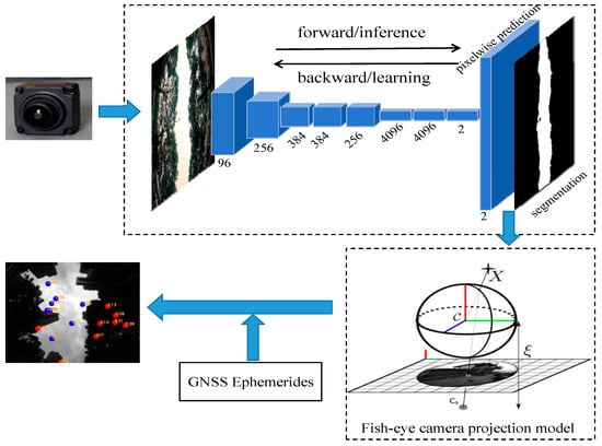
Figure 3.
The overall flow of S-NDM algorithm.
3. Experiments
This section delineates the experimental methodology undertaken to assess the effectiveness of sky-view image-assisted GNSS NLOS detection across different positioning models. The study categorizes the models into SPP-related and RTK-related tightly coupled models for a comparative analysis. To evaluate the positioning performance, we calculated the root mean square error (RMSE) in the three directions of east (E), north (N), and up (U).
3.1. Experiment Description
As is shown in Figure 4, the data acquisition platform consists of a GNSS receiver (Septentrio mosaic-X5 mini, Septentrio, Brussels, Belgium), GNSS antenna (NovAtel GNSS-850, NovAtel, Calgary, AB, Canada), two forward-looking cameras (FLIR BFS-U3-31S4C-C, FLIR Systems, Wilsonville, OR, USA), a sky-pointing fish-eye camera (FE185C057HA-1, FUJINON, Fuji, Japan), a tactical-grade IMU (NovAtel SPAN-ISA-100C, NovAtel , Calgary, AB, Canada), an MEMS-IMU (ADIS-16470, ADI, Boston, MA, USA), and a time synchronization board. The time synchronization board unifies the time of all sensors to GPS time through pulse per second (PPS) generated by the GNSS receiver. The sampling rates of GNSS, MEMS-IMU, forward-looking cameras, and fish-eye camera are 1 Hz, 100 Hz, 10 Hz, and 1 Hz, respectively. In addition, the NovAtel SPAN-ISA-100C interacts with NovAtel’s ProPak7 receiver via a highly reliable IMU interface. The tightly coupled multi-GNSS post-processing kinematic (PPK)/INS bidirectional smoothing position results can be obtained through commercial IE 8.9 software and used as a reference truth value. Table 1 lists the specific parameters of the two IMUs. We use the Linux operating system and an Intel Core i7-9750H processor running at 2.6 GHz and with 32 GB memory. In addition, the data are processed on a laptop with NVIDIA GeForce RTX 3060 Ti GPU (graphics processing unit) based on Ubuntu 18.04 (Canonical Ltd., London, UK). Meanwhile, we used opencv3.4.9 [39] to process the images in the tightly coupled system.
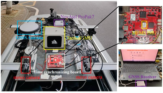
Figure 4.
Illustration of experimental hardware platform.

Table 1.
The parameters of the IMU sensors used in the vehicle experiments.
We collected vehicular data in a typical urban canyon area in Wuhan on 3 September 2023. The experimental trajectory and surrounding landscape, featuring high-rise structures, dense foliage, and overpasses, are illustrated in Figure 5. The number of satellites and the position dilution of precision (PDOP) values for this route are shown in Figure 6. Combined with the LOS/NLOS satellite conditions presented in Figure 5, it is conceivable that our testing environment is plagued by severe GNSS NLOS, multipath, and cycle slip issues. These complications not only impair GNSS−based positioning accuracy but also challenge the reliability of GNSS/INS/Vision integration model, which depends on GNSS for absolute position information. The choice of such a challenging environment underscores the purpose of the experiment, which is to validate the efficacy and dependability of S−NDM algorithm and Sky−GVIO model introduced in this study.
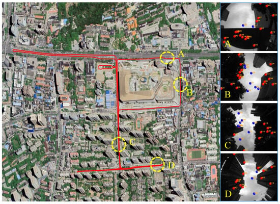
Figure 5.
The experimental route and scene in the urban canyon. ((A–D) on the right correspond to the sky-view images of the four scenes in the trajectory, respectively. In the sky-view images on the right, the red dots represent the NLOS satellite, and the blue dots represent the LOS satellite).
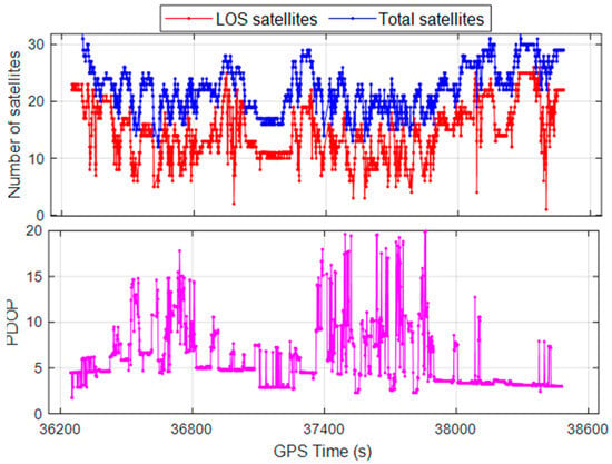
Figure 6.
Number of LOS satellites (top) and PDOP value of all satellites (bottom).
In addition, we briefly introduce our sky-view image dataset, including the training dataset and the testing dataset. The training dataset contains 440 images, and the testing dataset contains 2000 images, each with a resolution of 1432 × 1164 pixels. These data were collected in typical urban canyons in two different areas of Wuhan, which contain trees, tall buildings, and light poles. Therefore, this dataset is very suitable for sky-view image segmentation experiments. Figure 7 shows the sky-view images that we have labeled semantically, with blue representing the sky area and black representing the non-sky area.
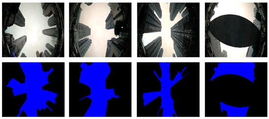
Figure 7.
Examples of sky-view image dataset annotated semantically. The first row is raw images (top), and the second row is semantic images (bottom).
3.2. The Results of Sky-View Image Segmentation and GNSS NLOS Detection
The segmentation of sky-view images in urban canyons is challenging due to dynamic environmental factors such as cloud cover and varying light conditions, which can degrade the accuracy of traditional image segmentation techniques. The result of poor image segmentation accuracy will lead to errors in NLOS detection. Figure 8 presents a comparison of the results of sky-view image segmentation between traditional segmentation algorithms and the method proposed in this paper.
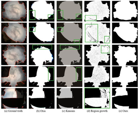
Figure 8.
Experimental results of sky-view image segmentation using different methods. From left to right: Ground truth with the outline of sky region (red line), followed by the segmentation results using Otsu, Kmeans, region growth, and our proposed method, respectively. Regions that are incorrectly segmented are highlighted in green boxes.
We compare our FCN−based method with representative image segmentation methods, including Otsu, Kmeans, and region growth. For fair comparison with the other competitors, all tests were performed on our collected dataset. As can be seen in Figure 8, clouds and light cause obvious errors in Figure 8b–d, especially in areas close to buildings. The performance of Otsu and Kmeans is relatively similar, but region growth shows a higher incidence of misclassification. Furthermore, in images featuring elevated bridges, an incorrect selection of seed points leads to the misidentification of sky regions as non-sky regions, which can be critically detrimental to NLOS identification. In contrast, our proposed FCN−based approach attains a high-precision segmentation outcome. This is because FCN captures global contextual information for the input image by using convolution and pooling layers. This allows the network to better understand the relationships between different objects and the overall structure of the image, which allows more accurate segmentation.
The FCN−derived segmentation results are utilized for NLOS detection, with the visibility of satellites illustrated in Figure 9. In Figure 9, we observe that there are no identification errors in the visualization results of LOS and NLOS satellites, underscoring the reliability of our S−NDM algorithm.
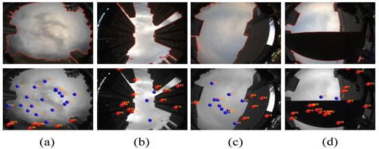
Figure 9.
(a–d) The detection visibility of LOS/NLOS satellites. (The red dots represent the NLOS satellite, and the blue dots represent the LOS satellite).
In the case of mild urban canyon environments (as shown in Figure 9a,c), LOS satellites dominate. However, in the case of deep urban canyons (as shown in Figure 9b) and environments with elevated bridges (as shown in Figure 9d), fewer than four LOS satellites are detectable, and the satellite configurations are suboptimal, highlighting the complexity and challenges of our experimental test environments.
3.3. The Quantitative Analysis of Sky-View Image Segmentation
Considering the strict requirements for precision and real-time measurements in vehicle positioning, we conducted quantitative tests on the efficiency and accuracy of different segmentation algorithms. The results are presented in Table 2. The efficiency of these algorithms is reflected by FPS (frames per second), which refers to the number of images processed per second. The accuracy of the algorithm is reflected by “Accuracy”, which refers to the percentage of the number of correctly segmented images in the total number of processing results. The experiment is carried out on the training dataset, which is convenient for us to calculate the performance index of these algorithms.
where denotes the number of pixels with correct sky region, denotes the number of pixels with correct non-sky region, denotes the number of pixels with incorrect sky region, and denotes the number of pixels with incorrect non-sky region.

Table 2.
Performance comparison of sky-view images using different methods.
It can be seen from Table 2 that the FCN−based image segmentation algorithm is more efficient, which is due to FCN supporting an acceleration in GPU processing. The accuracies of the other central processing unit (CPU)-based machine learning methods are less than 50%. In addition, the update cycle of the tightly coupled GNSS, INS, and Vision model based on MSCKF is 1 s (which is synchronized with the GNSS sampling frequency). Therefore, FCN’s FPS fully meets requirements. Compared with machine learning methods, FCN based on deep learning is also more advantageous in terms of accuracy. Therefore, in terms of efficiency or accuracy, the FCN−based sky-view image segmentation algorithm proposed in this paper is meaningful.
3.4. The Experimental Results of Positioning
To verify the effectiveness of the Sky−GVIO model for car positioning in the urban canyon region and to evaluate the performance improvement of the two modes based on SPP and RTK positioning enhanced by S−NDM, we conducted several experimental comparisons and compared the results with those of state-of-the-art methods. It should be noted that we use the RTK float solution.
The time series of position errors for different SPP−related tightly coupled models are shown in Figure 10, and the corresponding RMSEs are summarized in Table 3. The positioning accuracy of SPP/INS/Vision in E, N, and U directions is 3.24, 2.14, and 3.39 m. Different from SPP/INS/Vision, Sky−SPP/INS/Vision identifies LOS/NLOS satellites under the GNSS challenge environment and models them to inhibit the impact of NLOS on GNSS observations. As expected, the positioning accuracy is improved to 2.07, 1.51, and 2.47 m in E, N, and U directions when SPP/INS/Vision enhanced by S−NDM. Compared with SPP/INS/Vision, the positioning accuracy of Sky−SPP/INS/Vision is improved by 36%, 29%, and 27% in E, N, and U directions, respectively. As seen from results, Sky−SPP/INS/Vision can maintain meter-level positioning accuracy. Therefore, SPP−related Sky−GVIO is more suitable for mobile phone navigation and pedestrian navigation in urban canyons.
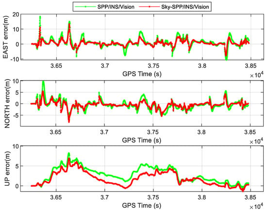
Figure 10.
Comparisons of the tightly coupled SPP/INS/Vision and Sky−SPP/INS/Vision models regarding position errors in urban canyon areas (Sky−SPP/INS/Vision refers to SPP−related Sky−GVIO).

Table 3.
Position RMSEs of VINS−mono, GVINS, SPP/INS/Vision, Sky−SPP/INS/Vision, RTK/INS/Vision, and Sky−RTK/INS/Vision models.
The time series of position errors for different tightly coupled RTK−related models are shown in Figure 11, and the corresponding RMSEs are summarized in Table 3. The positioning accuracy of RTK/INS/Vision in E, N, and U directions are 0.21, 0.13, and 0.36 m. It can be seen that the positioning accuracy of Sky−RTK/INS/Vision is 0.16, 0.11, and 0.27 m in E, N, and U directions, which outperforms RTK/INS/Vision. Compared with RTK/INS/Vision, the positioning accuracy of Sky−RTK/INS/Vision is improved by 24%, 15%, and 25% in E, N, and U directions, respectively. These considerable improvements in the positioning accuracy mainly stem from GNSS NLOS detection and mitigation enhanced by sky-view images, which makes the weighting of GNSS observations more reasonable. Meanwhile, we find that the S−NDM algorithm acts on SPP/INS/Vision better than RTK/INS/Vision in terms of positioning accuracy. This is because the positioning accuracy of SPP is lower than that of RTK positioning, and there is a lot of room for its enhancement; in addition, the NLOS has a greater effect on the pseudorange caused by the NLOS.
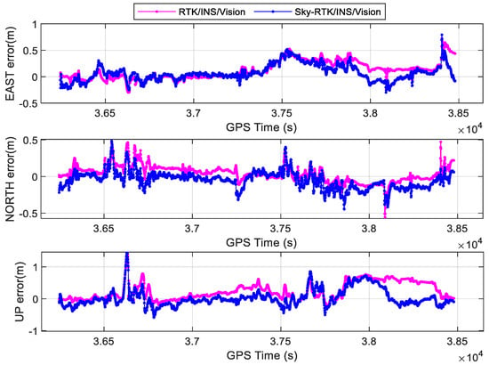
Figure 11.
Comparisons of the RTK/INS/Vision and Sky−RTK/INS/Vision models regarding position errors in urban canyon areas (Sky−RTK/INS/Vision refers to RTK−related Sky−GVIO).
In addition, we compared our results against those using state-of-the-art methods, including VINS−mono [8] and GVINS [10]. As we all know, VINS−mono is a very famous tightly coupled model. However, without external information for correction, VINS−mono will accumulate drift errors, resulting in gradually larger errors in E, N, and U directions as shown in Figure 12. Due to large errors obtained by VINS−mono, statistics are not shown in Table 3. GVINS, for which GNSS pseudorange measurement, GNSS doppler measurement, visual constraints, and inertial constraints were jointly optimized, is also mature tightly coupled GNSS/INS/Vision model, which is often used to compare models of the same type. The time series of position errors for GVINS are presented in Figure 13, and the corresponding RMSEs are summarized in Table 3. The positioning accuracy of GVINS in E, N, and U directions is 2.50, 1.75, and 2.82 m, which outperforms SPP/INS/Vision in this paper. This is because GVINS adds Doppler measurements. However, GVINS did not have strict quality control in GNSS preprocessing, especially in regards to GNSS NLOS. Therefore, Sky−SPP/INS/Vision model proposed in this paper has higher accuracy than GVINS.
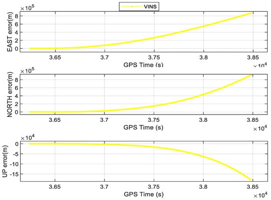
Figure 12.
The position errors of VINS−mono in E, N, and U directions.
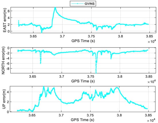
Figure 13.
The position errors of GVINS in E, N, and U directions.
4. Conclusions
To mitigate the impact of NLOS on GNSS observations, this paper proposes an S−NDM algorithm. The S−NDM employs an FCN to segment sky-view images, followed by satellite projection for NLOS detection. Building on this, S−NDM is integrated into a tightly coupled GNSS/INS/Vision positioning model, named Sky−GVIO. The experimental results show that the proposed S−NDM algorithm achieves a notable performance in terms of segmentation accuracy, efficiency, and NLOS detection. In addition, we also evaluate the positioning performance of various tightly coupled positioning methods, and the experimental results demonstrate that the proposed Sky−GVIO model effectively improves the positioning accuracy in urban canyons. Specifically, Sky−RTK/INS/Vision achieves sub-decimeter accuracy, which is highly valuable for users requiring high-precision positioning services, and Sky−SPP/INS/Vision achieves meter-level accuracy, which is beneficial for low-cost applications, such as smartphones and pedestrian navigation.
In the future, we still have the following work to do:
- (1)
- Enhance the utilization of fish-eye camera data beyond GNSS NLOS detection, potentially integrating fish-eye camera observations into the proposed model;
- (2)
- Reach centimeter-level accuracy. By adding prior information (such as high-precision maps), the whole system can be made more robust and the positioning accuracy can increase.
Author Contributions
Conceptualization, J.W. and J.L.; methodology, J.W.; software, J.W. and B.X.; validation, J.W. and S.Z.; data curation, J.W. and B.X.; writing—original draft preparation, J.W.; writing—review and editing, J.W., J.L., B.X. and K.G.; visualization, J.W.; supervision, J.L.; project administration, J.W.; funding acquisition, S.Z. All authors have read and agreed to the published version of the manuscript.
Funding
This work was supported by the National Key Research and Development Program of China under Grant 2021YFB2501100.
Data Availability Statement
The data in this paper are unavailable due to privacy or ethical restrictions.
Acknowledgments
We want to acknowledge Wenfei Guo for providing the time-synchronizing device.
Conflicts of Interest
The authors declare no conflicts of interest.
References
- Godha, S.; Cannon, M.E. GPS/MEMS INS integrated system for navigation in urban areas. GPS Solut. 2007, 11, 193–203. [Google Scholar] [CrossRef]
- Li, T.; Zhang, H.; Gao, Z.; Chen, Q.; Niu, X. High-accuracy positioning in urban environments using single-frequency multi-GNSS RTK/MEMS-IMU integration. Remote Sens. 2018, 10, 205. [Google Scholar] [CrossRef]
- Niu, X.; Dai, Y.; Liu, T.; Chen, Q.; Zhang, Q. Feature-based GNSS positioning error consistency optimization for GNSS/INS integrated system. GPS Solut. 2023, 27, 89. [Google Scholar] [CrossRef]
- Chen, K.; Chang, G.; Chen, C. GINav: A MATLAB-based software for the data processing and analysis of a GNSS/INS integrated navigation system. GPS Solut. 2021, 25, 108. [Google Scholar] [CrossRef]
- Xu, B.; Wang, P.; He, Y.; Chen, Y.; Chen, Y.; Zhou, M. Leveraging structural information to improve point line visual-inertial odometry. IEEE Robot. Autom. Lett. 2022, 7, 3483–3490. [Google Scholar] [CrossRef]
- He, Y.; Xu, B.; Ouyang, Z.; Li, H. A rotation-translation-decoupled solution for robust and efficient visual-inertial initialization. In Proceedings of the IEEE/CVF Conference on Computer Vision and Pattern Recognition, Vancouver, BC, Canada, 17–24 June 2023; pp. 739–748. [Google Scholar]
- Chen, Y.; Xu, B.; Wang, B.; Na, J.; Yang, P. GNSS Reconstrainted Visual–Inertial Odometry System Using Factor Graphs. IEEE Geosci. Remote Sens. Lett. 2023, 20, 1–5. [Google Scholar] [CrossRef]
- Qin, T.; Li, P.; Shen, S. Vins-mono: A robust and versatile monocular visual-inertial state estimator. IEEE Trans. Robot. 2018, 34, 1004–1020. [Google Scholar] [CrossRef]
- Liao, J.; Li, X.; Wang, X.; Li, S.; Wang, H. Enhancing navigation performance through visual-inertial odometry in GNSS-degraded environment. GPS Solut. 2021, 25, 50. [Google Scholar] [CrossRef]
- Cao, S.; Lu, X.; Shen, S. GVINS: Tightly coupled GNSS–visual–inertial fusion for smooth and consistent state estimation. IEEE Trans. Robot. 2022, 38, 2004–2021. [Google Scholar] [CrossRef]
- Mourikis, A.I.; Roumeliotis, S.I. A multi-state constraint Kalman filter for vision-aided inertial navigation. In Proceedings of the 2007 IEEE International Conference on Robotics and Automation, Rome, Italy, 10–14 April 2007. [Google Scholar] [CrossRef]
- Li, T.; Zhang, H.; Gao, Z.; Niu, X.; El-sheimy, N. Tight fusion of a monocular camera, MEMS-IMU, and single-frequency multi-GNSS RTK for precise navigation in GNSS-challenged environments. Remote Sens. 2019, 11, 610. [Google Scholar] [CrossRef]
- Groves, P.D.; Jiang, Z.; Skelton, B.; Cross, P.A.; Lau, L.; Adane, Y.; Kale, I. Novel multipath mitigation methods using a dual-polarization antenna. In Proceedings of the 23rd International Technical Meeting of The Satellite Division of the Institute of Navigation (ION GNSS 2010), Portland, OR, USA, 21–24 September 2010. [Google Scholar]
- Liu, S.; Li, D.; Li, B.; Wang, F. A compact high-precision GNSS antenna with a miniaturized choke ring. IEEE Antennas Wirel. Propag. Lett. 2017, 16, 2465–2468. [Google Scholar] [CrossRef]
- Gupta, I.J.; Weiss, I.M.; Morrison, A.W. Desired features of adaptive antenna arrays for GNSS receivers. Proc. IEEE 2016, 104, 1195–1206. [Google Scholar] [CrossRef]
- Won, D.H.; Ahn, J.; Lee, S.-W.; Lee, J.; Sung, S.; Park, H.-W.; Park, J.-P.; Lee, Y.J. Weighted DOP with consideration on elevation-dependent range errors of GNSS satellites. IEEE Trans. Instrum. Meas. 2012, 61, 3241–3250. [Google Scholar] [CrossRef]
- Groves, P.D.; Jiang, Z. Height aiding, C/N0 weighting and consistency checking for GNSS NLOS and multipath mitigation in urban areas. J. Navig. 2013, 66, 653–669. [Google Scholar] [CrossRef]
- Wen, W.; Zhang, G.; Hsu, L.-T. Exclusion of GNSS NLOS receptions caused by dynamic objects in heavy traffic urban scenarios using real-time 3D point cloud: An approach without 3D maps. In Proceedings of the 2018 IEEE/ION Position, Location and Navigation Symposium (PLANS), Monterey, CA, USA, 23–26 April 2018. [Google Scholar] [CrossRef]
- Wen, W.W.; Zhang, G.; Hsu, L.-T. GNSS NLOS exclusion based on dynamic object detection using LiDAR point cloud. IEEE Trans. Intell. Transp. Syst. 2019, 22, 853–862. [Google Scholar] [CrossRef]
- Wang, L.; Groves, P.D.; Ziebart, M.K. GNSS shadow matching: Improving urban positioning accuracy using a 3D city model with optimized visibility scoring scheme. NAVIGATION J. Inst. Navig. 2013, 60, 195–207. [Google Scholar] [CrossRef]
- Hsu, L.-T.; Gu, Y.; Kamijo, S. 3D building model-based pedestrian positioning method using GPS/GLONASS/QZSS and its reliability calculation. GPS Solut. 2016, 20, 413–428. [Google Scholar] [CrossRef]
- Suzuki, T.; Kubo, N. N-LOS GNSS signal detection using fish-eye camera for vehicle navigation in urban environments. In Proceedings of the 27th International Technical Meeting of the Satellite Division of the Institute of Navigation (ION GNSS+ 2014), Tampa, FL, USA, 8–12 September 2014. [Google Scholar]
- Wen, W.; Bai, X.; Kan, Y.C.; Hsu, L.T. Tightly coupled GNSS/INS integration via factor graph and aided by fish-eye camera. IEEE Trans. Veh. Technol. 2019, 68, 10651–10662. [Google Scholar] [CrossRef]
- Meguro, J.-i.; Murata, T.; Takiguchi, J.I.; Amano, Y.; Hashizume, T. GPS multipath mitigation for urban area using omnidirectional infrared camera. IEEE Trans. Intell. Transp. Syst. 2009, 10, 22–30. [Google Scholar] [CrossRef]
- Cohen, A.; Meurie, C.; Ruichek, Y.; Marais, J.; Flancquart, A. Quantification of gnss signals accuracy: An image segmentation method for estimating the percentage of sky. In Proceedings of the 2009 IEEE International Conference on Vehicular Electronics and Safety (ICVES), Pune, India, 11–12 November 2009. [Google Scholar] [CrossRef]
- Attia, D.; Meurie, C.; Ruichek, Y.; Marais, J. Counting of satellites with direct GNSS signals using Fisheye camera: A comparison of clustering algorithms. In Proceedings of the 2011 14th International IEEE Conference on Intelligent Transportation Systems (ITSC), Washington, DC, USA, 5–7 October 2011. [Google Scholar] [CrossRef]
- Wang, J.; Liu, J.; Zhang, S.; Xu, B.; Luo, Y.; Jin, R. Sky-view images aided NLOS detection and suppression for tightly coupled GNSS/INS system in urban canyon areas. Meas. Sci. Technol. 2023, 35, 025112. [Google Scholar] [CrossRef]
- Vijay, P.; Patil, N.C. Gray scale image segmentation using OTSU Thresholding optimal approach. J. Res. 2016, 2, 20–24. [Google Scholar]
- Dhanachandra, N.; Manglem, K.; Chanu, Y.J. Image segmentation using K-means clustering algorithm and subtractive clustering algorithm. Procedia Comput. Sci. 2015, 54, 764–771. [Google Scholar] [CrossRef]
- Soltani-Nabipour, J.; Khorshidi, A.; Noorian, B. Lung tumor segmentation using improved region growing algorithm. Nucl. Eng. Technol. 2020, 52, 2313–2319. [Google Scholar] [CrossRef]
- Long, J.; Shelhamer, E.; Darrell, T. Fully convolutional networks for semantic segmentation. In Proceedings of the IEEE Conference on Computer Vision and Pattern Recognition, Boston, MA, USA, 7–12 June 2015. [Google Scholar]
- He, K.; Zhang, X.; Ren, S.; Sun, J. Deep residual learning for image recognition. In Proceedings of the IEEE Conference on Computer Vision and Pattern Recognition, Las Vegas, NV, USA, 27–30 June 2016; pp. 770–778. [Google Scholar]
- Xu, B.; Zhang, S.; Kuang, K.; Li, X. A unified cycle-slip, multipath estimation, detection and mitigation method for VIO-aided PPP in urban environments. GPS Solut. 2023, 27, 59. [Google Scholar] [CrossRef]
- Furgale, P.; Rehder, J.; Siegwart, R. Unified temporal and spatial calibration for multi-sensor systems. In Proceedings of the 2013 IEEE/RSJ International Conference on Intelligent Robots and Systems, Tokyo, Japan, 3–7 November 2013; pp. 1280–1286. [Google Scholar] [CrossRef]
- Sun, K.; Mohta, K.; Pfrommer, B.; Watterson, M.; Liu, S.; Mulgaonkar, Y.; Taylor, C.J.; Kumar, V. Robust stereo visual inertial odometry for fast autonomous flight. IEEE Robot. Autom. Lett. 2018, 3, 965–972. [Google Scholar] [CrossRef]
- Rehder, J.; Nikolic, J.; Schneider, T.; Hinzmann, T.; Siegwart, R. Extending kalibr: Calibrating the extrinsics of multiple IMUs and of individual axes. In Proceedings of the 2016 IEEE International Conference on Robotics and Automation (ICRA), Stockholm, Sweden, 16–21 May 2016. [Google Scholar] [CrossRef]
- Sola, J. Quaternion kinematics for the error-state Kalman filter. arXiv 2017, arXiv:1711.02508. [Google Scholar] [CrossRef]
- Herrera, A.M.; Suhandri, H.F.; Realini, E.; Reguzzoni, M.; de Lacy, M.C. goGPS: Open-source MATLAB software. GPS Solut. 2016, 20, 595–603. [Google Scholar] [CrossRef]
- Bradski, G. The OpenCV Library. Dr. Dobb’s J. Softw. Tools 2000, 120, 122–125. Available online: https://opencv.org (accessed on 4 April 2023).
Disclaimer/Publisher’s Note: The statements, opinions and data contained in all publications are solely those of the individual author(s) and contributor(s) and not of MDPI and/or the editor(s). MDPI and/or the editor(s) disclaim responsibility for any injury to people or property resulting from any ideas, methods, instructions or products referred to in the content. |
© 2024 by the authors. Licensee MDPI, Basel, Switzerland. This article is an open access article distributed under the terms and conditions of the Creative Commons Attribution (CC BY) license (https://creativecommons.org/licenses/by/4.0/).