From Spectral Characteristics to Index Bands: Utilizing UAV Hyperspectral Index Optimization on Algorithms for Estimating Canopy Nitrogen Concentration in Carya Cathayensis Sarg

Abstract

Employing drones and hyperspectral imagers for large-scale, precise evaluation of nitrogen (N) concentration in Carya cathayensis Sarg canopies is crucial for accurately managing nitrogen fertilization in C. cathayensis Sarg cultivation. This study gathered five sets of hyperspectral imagery data from C. cathayensis Sarg plantations across four distinct locations with varying environmental stresses using drones. The research assessed the canopy nitrogen concentration of C. cathayensis Sarg trees both during singular growth periods and throughout their entire growth cycles. The objective was to explore the influence of band combinations and spectral index formula configurations on the predictive capability of the hyperspectral indices (HIs) for canopy N concentration (CNC), optimize the performance between HIs and machine learning approaches, and validate the efficacy of optimized HI algorithms. The findings revealed the following: (i) Optimized HIs demonstrated optimal predictive performance during both singular growth periods and the full growth cycles of C. cathayensis Sarg. The most effective HI model for singular growth periods was the optimized–modified–normalized difference vegetation index (opt-mNDVI), achieving an adjusted coefficient of determination (R²) of 0.96 and a root mean square error (RMSE) of 0.71. For the entire growth cycle, the HI model, also opt-mNDVI, attained an R² of 0.75 and an RMSE of 2.11; (ii) optimized band combinations substantially enhanced HIs’ predictive performance by 16% to 71%, while the choice between three-band and two-band combinations influenced the predictive capacity of optimized HIs by 4% to 46%. Hence, utilizing optimized HIs combined with Unmanned Aerial Vehicle (UAV) hyperspectral imaging to evaluate nitrogen concentration in C. cathayensis Sarg trees under complex field conditions offers significant practical value.

1. Introduction

C. cathayensis Sarg is one of the classic examples of China’s economic forest crops, revered as a native high-quality dry fruit and woody oilseed crop [1].

Belonging to the walnut family, this perennial deciduous fruit tree is predominantly grown in the provinces of Zhejiang and Anhui [2]. With its high added value and health benefits, the cultivation of C. cathayensis Sarg is becoming increasingly popular as an ideal agricultural choice. Nitrogen (N) is an essential element that influences the growth, yield, and quality of fruit trees. The amount of nitrogen applied is intricately connected to the yield and quality of C. cathayensis Sarg, forming an integral part of its cultivation and management. It provides the tree with a range of necessary nutrients. However, in the pursuit of economic benefits, farmers frequently resort to the overuse of nitrogen. This excessive application not only adversely affects the yield and quality of the hickory but also disrupts the nutritional balance of the plants, potentially leading to plant death and environmental pollution issues. To mitigate this problem, monitoring the nitrogen concentration in C. cathayensis Sarg is imperative to provide guidance on fertilization and cultivation management to farmers.

Traditional chemical analysis [3,4,5,6], due to its time-consuming nature and high cost, is unsuitable for extensive monitoring of C. cathayensis Sarg, proving impractical for both researchers and farmers alike [7]. Remote sensing technology offers a superior alternative to traditional laboratory diagnostics by enabling the acquisition of vegetation’s spectral data to predict crops’ physicochemical characteristics. Hyperspectral remote sensing has revolutionized the field by combining spectroscopic techniques with traditional remote sensing, significantly expanding the spectral dimension of remote sensing imagery beyond the mere spatial dimension. This technological advancement allows for hyperspectral imagery to present highly diagnostic spectral curves for pixels, showcasing the unique reflective features of various terrestrial objects across a broad spectrum of continuous bands. This facilitates a more nuanced extraction and utilization of the minute differences among these features in hyperspectral remote sensing image analysis. Numerous studies have validated the superior capability of hyperspectral remote sensing in monitoring the nitrogen status of crop vegetation, with applications ranging from satellite hyperspectral technology [8,9,10] for extensive area coverage in large-scale crop health monitoring to UAV hyperspectral imaging [11,12] for detailed, high-resolution vegetation analysis, and even field-based studies using handheld hyperspectral devices [13,14,15]. These diverse application methods have synergistically contributed to the evolution of precision agriculture, with UAV hyperspectral technology playing a crucial role in the remote sensing monitoring of forestry due to its high efficiency, cost-effectiveness, and accuracy. At the same time, C. cathayensis Sarg trees are typically planted on steep mountain slopes and hillsides, with tall tree structures and complex terrain, making manual monitoring costly and high-risk. Drone monitoring can significantly reduce labor costs and risks. Compared to satellite remote sensing, drones offer higher spatial resolution, enabling the capture of detailed characteristics of individual trees and providing high-quality spectral information, which is especially important for analyzing local variations in nitrogen levels.

In the realm of hyperspectral remote sensing for monitoring vegetation’s physicochemical traits, vegetation indices (VIs) and both linear and non-linear regression analyses stand as cornerstone methodologies in the assessment of crops’ biochemical conditions. These strategies are prevalently utilized for deriving various parameters, including nitrogen concentration. While traditional indices such as the normalized difference vegetation index (NDVI) [16] and enhanced vegetation index (EVI) have achieved notable success in gauging vegetation cover and health, they fall short of exploiting the comprehensive detail and depth that hyperspectral data afford. In pursuit of bolstering the predictive accuracy of vegetation characteristics via hyperspectral indices, an array of formulaic variations of HIs has been introduced. Notably, some researchers [17] proposed the soil-adjusted vegetation index (SAVI), followed by the development of the modified soil-adjusted vegetation index (MSAVI) and optimized soil-adjusted vegetation index (OSAVI) in subsequent research [18,19]. Additionally, studies [20] have formulated a variety of hyperspectral indices based on canopy or leaf spectral reflectance, extensively applied in forecasting the canopy nitrogen condition of crops.

The swift advancements in hyperspectral remote sensing technology, bolstered by high-resolution hyperspectral instrumentation, offer an expanded array of potential bands for creating hyperspectral indices (HIs) [21]. As a result, the optimization of HIs emerges as particularly crucial. By formulating novel or improved spectral indices, the subtle distinctions residing within hyperspectral data can be more proficiently seized, fostering a more precise evaluation of plant physiological states and nutritional requisites. However, the predicament resides in distinguishing the optimal band amalgamation within the confines of a specified HI formula. A favored approach entails calculating all plausible band combinations contingent upon the established HI formula [22]. For instance, some researchers [23] undertook an exhaustive analysis of all NDVI band combinations traversing from 350 nm to 1050 nm, enhancing the predictive potential of the optimized NDVI in turn. Likewise, through examining the responsiveness of the canopy nitrogen concentration (CNC) of Solanum tuberosum L. plants to band optimization and formulaic formats. Another study [24] constructed optimized HIs which notably ameliorated HI performance compared to previously documented HIs.

Confronting the array of challenges inherent in the application of hyperspectral technology, this study is dedicated to the development and validation of vegetation indices that are fine-tuned to meet specific requirements, thereby harnessing hyperspectral data more effectively for the surveillance and evaluation of vegetation health, with a keen focus on precision agriculture and the management of economic forests. The central aims of this research are threefold: 1. to refine existing hyperspectral indices (HIs); 2. to ascertain the contributions of band optimization and formulaic configurations in the appraisal of C. cathayensis Sarg; and 3. to corroborate the efficacy of the optimized HIs. By defining these objectives, this study aspires to transcend the confines of current technologies, amplifying the tangible utility of hyperspectral technology within the spheres of agricultural production and forest resource governance. This initiative is pivotal not only for elevating crop yields and quality but also bears profound significance for the stewardship of the ecological milieu and the advancement of sustainable practices.

2. Materials and Methods

2.1. Study Area Overview and Experimental Design

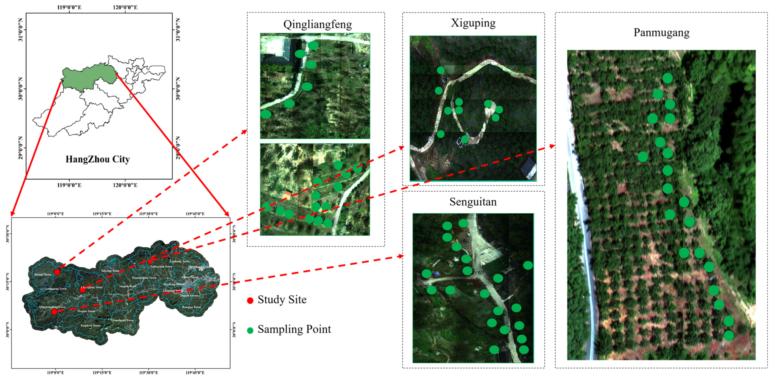
The research locale is situated in Lin’an District, Hangzhou City, Zhejiang Province, China, spanning the geographical coordinates from 118°51′E to 119°52′E and from 29°56′N to 30°23′N. The experimental area is shown in Figure 1. The regional climate embodies the subtropical monsoon meteorological pattern with sweltering summers, temperate winters, clearly delineated seasonal cycles, and a pronounced monsoon presence. This study has handpicked four experimental plantations—Xiguping, Senguitang, Qiliangfeng, and Panmugang—principally dedicated to the cultivation of the Lin’an hickory. Situated, respectively, in Changhua Town, Dashizhen, Qiliangfeng Town, and Taihu Yuan Town within the confines of Lin’an, these four plantation sites are quintessential exemplars of local C. cathayensis Sarg cultivation.

The inaugural experiment took place during the 2022 season of prolific fruiting and subsequent fruit fall of the C. cathayensis Sarg. A total of 50 samples were collected in 2022. Leaf samples were gathered from a collective count of 50 trees across three experimental sites, apportioned as 10, 20, and 20 trees, respectively; for each tree, 5 to 10 healthy leaves were collected from the east, south, west, and north sides, as well as from the upper, middle, and lower layers of the tree. Additionally, the leaves were required to be intact and free of visible damage. The year’s overarching climatic conditions brought drought to all three sites. In Lin’an District, despite 22 rainy days between August and September, the accumulated rainfall only amounted to a scant 45.8mm, failing to satisfy the hydration requisites of the hickory crops. As a result, the hickory’s fundamental moisture needs were predominantly supplemented through artificial irrigation. Through field surveys and consultations with local cultivators and hickory connoisseurs, it was gleaned that Senguitang, with its adequate staffing, maintained optimal daily irrigation and thus was minimally affected by the drought. In contrast, Xiguping, with its personnel deficit, managed irrigation merely every two to three days, whereas the Qiliangfeng site, hindered by its lofty terrain and the inconvenience it posed to manual watering, went without irrigation. Post-expert deliberation, the drought stress experienced by the sites was stratified into three tiers: high, medium, and low. Subsequently, the second experiment was executed in 2023 at the Panmugang site in Lin’an District. A sufficient number of leaf samples were collected from the canopy of 20 C. cathayensis Sarg trees on 27 April and 12 July of that year, under the aegis of untroubled weather conditions devoid of calamitous influences.

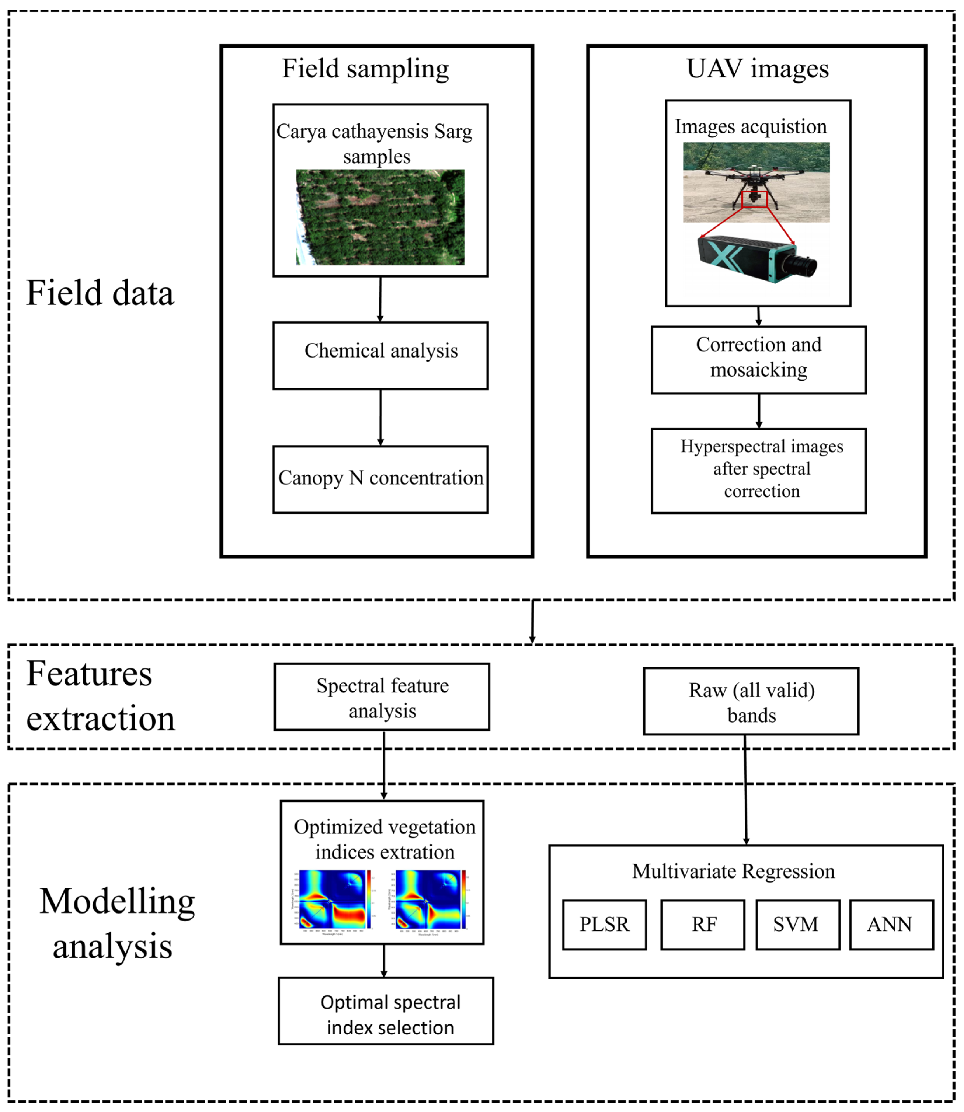
In all areas, a complex fertilizer with a nutrient ratio of N:P2O5:K2O = 15:15:15 is utilized, and delivered at an application rate of 375 kg per hectare. The fertilization process involves a scattering method beneath the forest canopy, with each C. cathayensis Sarg tree receiving approximately 3 kg of fertilizer per plant. The fertilization phase is initiated in mid-March in all areas. However, with Xiguping being the exception, an extra round of fertilization is introduced at the onset of September in the other regions, whilst maintaining a consistent application rate. The main research process is shown in Figure 2.

2.2. Experiment Management and Data Extraction

2.2.1. Acquisition of UAV-Based Hyperspectral Images

A UAV equipped with a hyperspectral imaging system was utilized for the collection of visible–infrared hyperspectral data. The system components include the UAV (DJI M600Pro, SZ DJI Technology Co., Ltd., Shenzhen, China), an HY-1230 hyperspectral camera (Hangzhou Hyperspectral Imaging Technology Co., Ltd., Hangzhou, China), a two-axis gimbal, and an onboard control and data acquisition system. The main parameters of the equipment are shown in

Table 1. Image data acquisition equipment parameters.

Parameters	Values
Wavelength	400–1000 nm
Lens	12.5 mm/25 mm/35 mm
Sampling interval	2.8 nm
Pixel inteval	5.86 μm
Field of view	15.6°@f = 35 mm

. During flight missions, the altitude was set at 100 m, and both heading overlap and sidelap were configured at 94.5% and 82%, respectively. The hyperspectral imaging camera featured 300 spectral channels, covering a wavelength range of 350–1000 nm, with a spectral resolution surpassing 2.8 nm and a sampling interval of 0.5 nm.

Canopy reflectance measurements for C. cathayensis Sarg trees were conducted at the Xiguping experimental site on 29 August 2022, at the Senguitang experimental site on 29 September, and at the Qiliangfeng experimental site on 30 September. In the following year, on 27 April and 12 July 2023, canopy reflectance measurements for hickory trees were conducted at the Panmugang experimental site. All readings were recorded between 10:00 AM and 2:00 PM during the key growth seasons of the trees under conditions of clear skies. This period coincides with the fruiting season of C. cathayensis Sarg, where the fruits are ripe, and the nitrogen concentration in both leaves and fruits remains relatively stable. The UAV is programmed to follow a specific flight path at an altitude of 100m and a speed of 3.6m/s to capture hyperspectral data of the C. cathayensis Sarg forest. Concurrently, based on the latitude and longitude coordinates of ground sample points, corresponding feature points are identified on the images.

2.2.2. Collection of Leaf Samples and Laboratory Measurement of Leaf Nitrogen Content (LNC)

For each sampled plant, leaf excision was carried out at different orientations and heights. The excised leaves were carefully labeled, stored, and transported back to the laboratory for subsequent chemical analysis. Within the lab setting, each specimen was first subjected to a drying phase at temperatures ranging from 100 to 110 °C and lasting for 15–30 min; then, each specimen proceeded to undergo prolonged desiccation at 70–80 °C for a duration of 4–8 h to attain a stable mass. The desiccated foliage was then pulverized, filtered through a sieve with a 1 mm mesh, and preserved in polyethylene containers. LNC (%) was quantified using the Kjeldahl method with a DH5180 intelligent integrated distillation instrument (Dehe Chuangrui, Qingdao, China).

Figure 3 depicts the nitrogen concentration in C. cathayensis Sarg leaves under five varying conditions, clearly demonstrating significant differences in nitrogen levels between different areas. We conducted variance analysis for the 5 sets of data, including the original 3 groups of nitrogen content data. The result was p = 2.07 × 10⁻³⁰, significantly less than 0.05, which indicates that there are significant differences among these groups of data. These differences originate from variable fertilization quantities and external environmental influences.

2.3. Spectral Pretreatment Method

In this study, an image processing pipeline was utilized to extract the average reflectance spectra of individual C. cathayensis Sarg tree canopies. The initial step involved calibrating the raw data using standard reflectance, and bands above 930 nm were excluded from the original spectra due to lower spectral quality. Subsequently, the pixel range corresponding to the canopy was segmented from the background, and the average spectrum for each canopy was computed. UAV image stitching and canopy extraction were performed using ENVI Classic 5.3.

2.3.1. Canopy Extraction

To reduce the influence of background disturbances on the reflectance spectra, we employed the Savitzky–Golay smoothing algorithm as a preprocessing step for the spectral data. A quintic polynomial of second order, coupled with a 31-point smoothing window, was implemented for curve fitting and noise reduction purposes. An algorithm in two stages was employed to isolate plant reflectance from soil interference, utilizing NDVI to differentiate vegetative pixels within the hyperspectral data cube. The NDVI image was generated by calculating the normalized difference between the wavelengths of 750 nm and 650 nm for each pixel, which is shown in Equation (1).

$$\mathrm{NDVI}={\displaystyle \frac{{\mathrm{I}}_{750}-{\mathrm{I}}_{650}}{{\mathrm{I}}_{750}+{\mathrm{I}}_{650}}}$$

(1)

Here, I₇₅₀ and I₆₅₀ denote the spectral reflectance of pixels at 750 nm and 650 nm, respectively.

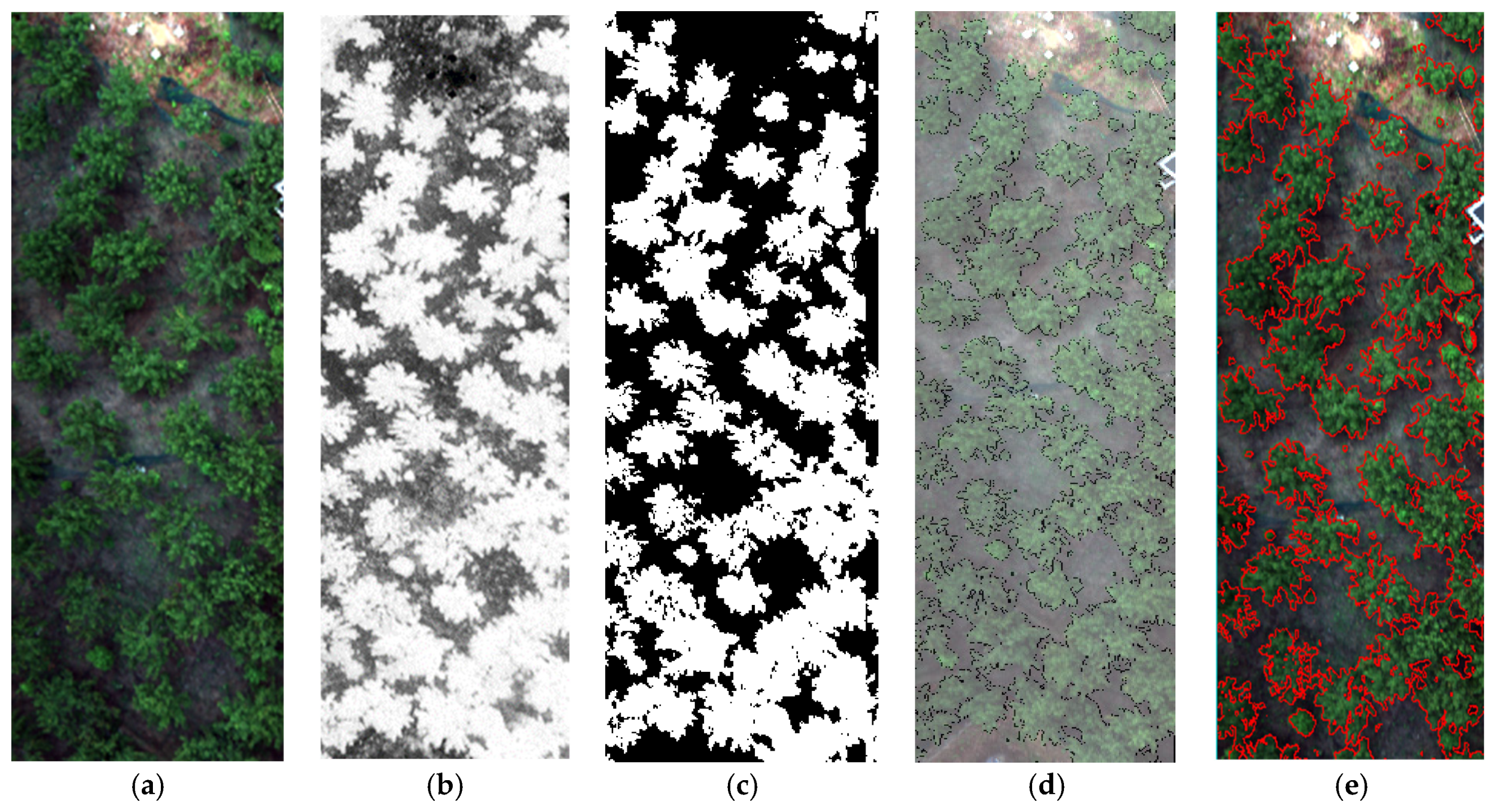
The Otsu algorithm was utilized to ascertain the pixel segmentation threshold for NDVI, which is shown in Figure 4, resulting in a mask for canopy extraction. However, the segmentation process may introduce some noise points, leading to the potential loss of canopy pixels. To address this, a straightforward Gaussian filtering method was employed to smooth the segmentation results, as depicted in the figure. Lastly, the coordinates of the sampled targets, acquired through GPS, were employed to pinpoint their positions on the hyperspectral image.

2.3.2. Hyperspectral Indices

To investigate the effects of different hyperspectral indices (HIs) on the assessment of CNC in the foliage of C. cathayensis Sarg, we opted for 21 algorithms documented in the literature (

Table 2. Algorithms for the hyperspectral indices utilized in this study.

Acronym	Spectral Indices	Formulas	References
CIred-edge	Red-edge chlorophyll index	(Ri − Rj)/Rj	[25]
DVI	Different vegetation index	Ri − Rj	[26]
MSAVI	Modified soil-adjusted vegetation index	0.5 × (2 × Ri + 1 − ((2 × Rj + 1)2 – 8 × (Ri − Rj))0.5	[18]
NDVI	Normalized difference vegetation index	(Ri − Rj)/(Ri + Rj)	[16]
OSAVI	Optimized soil-adjusted vegetation index	1.16 × (Ri − Rj)/(Ri + Rj + 0.16)	[19]
RVI	Ratio vegetation index	Ri/Rj	[27]
RDVI	The renormalized difference vegetation index	(Ri − Rj)/sqrt(Ri + Rj)	[28]
SAVI	Soil-adjusted vegetation index	1.5 × (Ri − Rj)/(Ri + Rj + 0.5)	[17]
VIopt	Optimal vegetation index	(1 + 0.45) × ((Ri)2 + 1)/(Rj + 0.45)	[29]
BNI1	Blue nitrogen index 1	Ri/(Rj + Rk)	[30]
BNI2	Blue nitrogen index 2	(Ri + Rj)/Rk	[30]
mSR705	Modified red-edge ratio	(Ri − Rj)/(Rk − Rj)	[31]
mNDVIblue	Modified–normalized difference vegetation index	(Ri − Rj + 2 × Rk)/(Ri + Rj − 2 × Rk)	[32]
Mrer	Modified red-edge ratio	(Ri − 1.8 × Rj)/(Rk − 1.8 × Rj)	[33]
MTCI	The MERIS terrestrial chlorophyll index	(Ri − Rj)/(Rj − Rk)	[34]
MTVI1	Modified triangular vegetation index 1	1.2 × [1.2 × (Ri − Rj) − 2.5 × (Rk − Rj)]	[35]
MCARI	Modified chlorophyll absorption reflectance index	[(Ri − Rj) − 0.2 × (Ri − Rk)] × (Ri/Rj)	[36]
NDDA	Double-peak nitrogen index	(Ri + Rj − 2 × Rk)/(Ri − Rj)	[37]
PSRI	Plant senescence reflectance index	(Ri − Rj)/Rk	[38]
TRSI	Three-band ratio spectral index	Ri/(Rj × Rk)	[39]
TVI	Triangle vegetation index	0.5 × (120 × (Ri − Rj) – 200 × (Rk − Rj))	[40]

). These algorithms rely on diverse combinations of bands in the visible and near-infrared spectra (wavelengths ranging from 400 to 930 nm) and are designed to extract information from hyperspectral data. To refine these algorithms, we considered all possible combinations of two and three wavelengths and conducted thorough data processing and analysis.

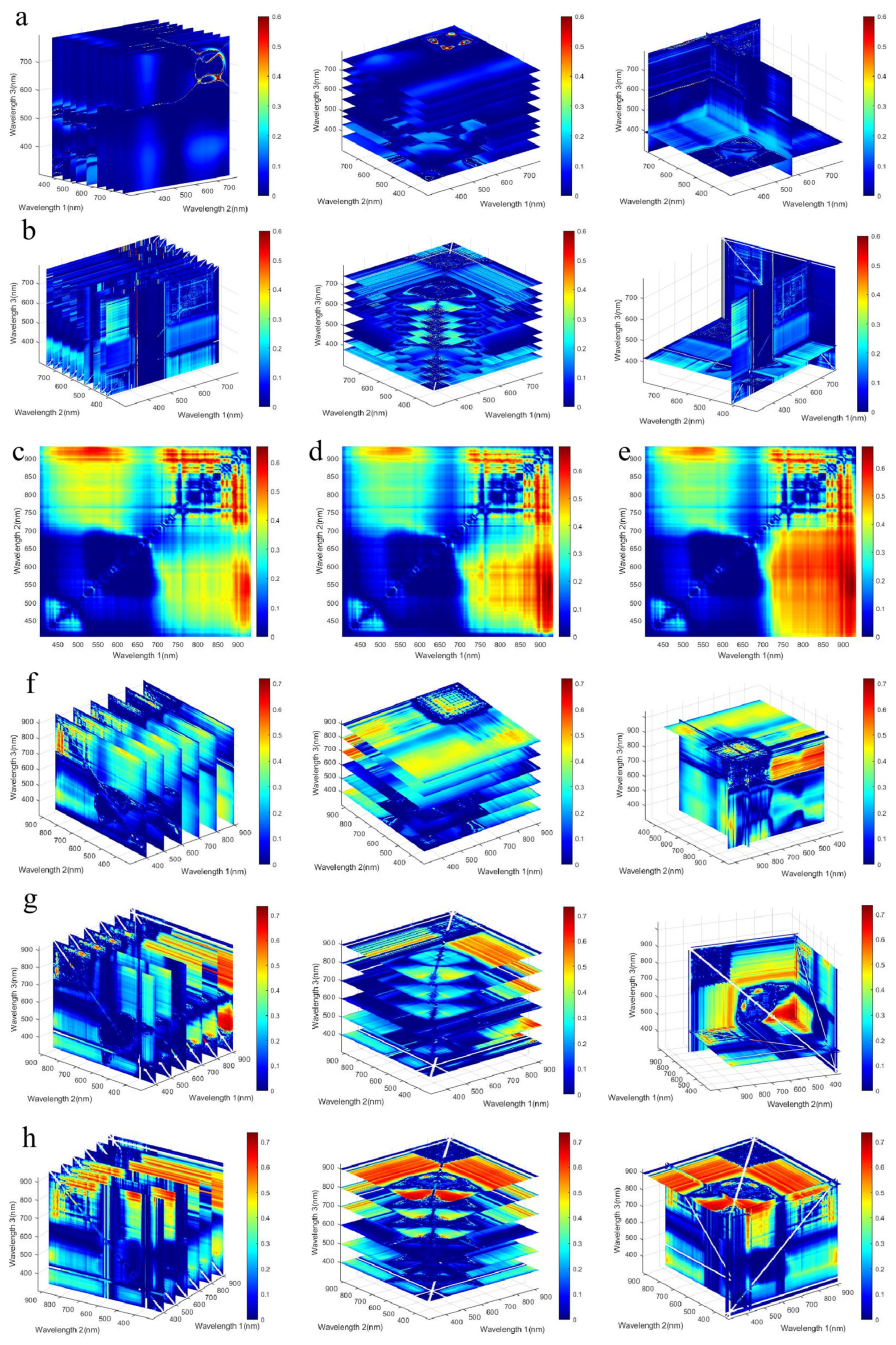
Throughout the study, we generated 2D and 3D contour plots, as well as slice plots, to visually depict the relationship between optimized HIs and CNC. These graphical representations serve to enhance our comprehension of how different hyperspectral index algorithms impact the performance of CNC estimation.

In the range of 400 nm to 930 nm, Ri, Rj and R_k represent any spectral wavelengths within this range.

2.4. Modeling Method

The experimental computation was carried out in the MATLAB environment. The workstation involved in this study was equipped with an Intel^® Xeon(R) Silver 4216 CPU running at 2.10 GHz across 32 cores and an Nvidia GeForce RTX 3090 GPU. The algorithms utilized comprised Partial Least Squares Regression (PLSR), support vector machines (SVMs), artificial neural networks (ANNs), and random forest (RF). We established linear regression models based on both publicly available spectral indices and optimized spectral indices. By leveraging the GPU’s parallel computing capabilities, we successfully enhanced computational speed and efficiency. This enhancement was achieved by reducing data transfer time and incorporating strategies such as loop parallelization and vectorized operations.

The study assessed 21 HIs commonly employed for estimating biomass, chlorophyll, and nitrogen status. Additionally, for this research, an artificial neural network employed a single hidden layer structure, while the support vector machine utilized a radial basis kernel function (RBF). Within these methods, hyperparameters such as latent variables in PLSR (lv), hidden units in artificial neural networks (units), for each tree within the random forest (mtry), the quantity of trees, the standard deviation (σ) in the radial basis function (RBF), and the regularization parameter c in the support vector machine’s (SVM) Lagrangian formulation demanded meticulous adjustment.

2.5. Evaluation of Model Performance

The datasets with 50 and 90 samples were divided into calibration and validation sets in a 3:2 ratio, respectively. Each model was calibrated and validated on its designated dataset. The performance of the models was assessed by employing metrics such as RE, RMSE, and R².

$${\mathrm{R}}^2={\displaystyle \frac{{{\displaystyle \sum }}_{\mathrm{i}=1}^{\mathrm{n}}{\left({\mathrm{y}}_{\mathrm{i}}^{\wedge }- \stackrel{-}{\mathrm{y}}\right)}^2}{{{\displaystyle \sum }}_{\mathrm{i}=1}^{\mathrm{n}}{\left({\mathrm{y}}_{\mathrm{i}}-\stackrel{-}{\mathrm{y}}\right)}^2}}$$

(2)

$$\mathrm{RMSE}=\sqrt{{\displaystyle \frac{1}{\mathrm{n}}}}{{\displaystyle \sum }}_{\mathrm{i}-1}^{\mathrm{n}}{\left({\mathrm{y}}_{\mathrm{i}}^{^}-{\mathrm{y}}_{\mathrm{i}}\right)}^2$$

(3)

$$\mathrm{RE}\left(\%\right)={\displaystyle \frac{\mathrm{RMSE}}{\stackrel{-}{\mathrm{y}}}}\ast 100$$

(4)

Evaluation of Hyperspectral Index Performance

The Noise Equivalent (NE) method was utilized to assess the sensitivity of different optimized HIs in predicting CNC, as expressed in the formula:

NE = RMSE{HIsvs.CNC}/[d(HIs)/d(CNC)]

(5)

Evaluating the model’s performance in predicting CNC through the NE value can reveal the model’s sensitivity to different HIs across various spectral bands. The NE value represents the ratio of the prediction error (RMSE) to the rate of change of the index relative to the change in CNC. Therefore, a lower NE value indicates a higher sensitivity of the HIs to variations in CNC, meaning the model is more precise in capturing fluctuations in CNC. The evaluation of the model was conducted by comparing the forecasted R², RMSE, and Relative Error (RE, as a percentage). Superior model performance is reflected by a higher R² and lower values of RMSE and RE, which are indicative of more accurate and stable predictions of CNC.

Model stability is a key criterion for evaluating the models’ application potential. In this study, the stability of models in estimating CNC was evaluated by considering leaf chlorophyll content and leaf area index (LAI). The PROSAIL model combines PROSPECT and SAIL to simulate the spectral reflectance characteristics of plant canopies, generating precise, controllable, and efficient spectral data, and enabling systematic evaluation, optimization, and validation of CNC inversion models. Nitrogen content in plants is moderately to highly correlated with chlorophyll content. To examine the relationship between different models and CNC, the PROSAIL model generated simulated datasets under specific conditions, with a step size of 10 µg·cm⁻² and chlorophyll content ranging from 10 to 60 µg·cm⁻². The PROSAIL model (

Table 3. The ranges of the input parameters for the PROSAIL model.

Parameter	Min	Max
Leaf structure parameter	1.3	2
Equivalent water thickness (cm)	0.005	0.03
Leaf mass per area (g/cm2)	0.004	0.01
Leaf area index (m2/m2)	1	8
Average leaf angle (deg)	30	70
Soil moisture parameter	0	1
Hot spot size parameter (deg)	0.05	1
Solar zenith angle (deg)	30	60
View zenith angle (deg)	0	0
View azimuth angle (deg)	0	0

) simulated 1000 effective spectral reflectance data points. The assessment of model robustness was conducted by analyzing the coefficient of variation (CV) and the coefficient of determination (R²) across distinct models using synthesized spectral data, thereby gauging the effects of CNC and LAI fluctuations on model accuracy. Enhanced stability in the model’s CNC estimations is evidenced by an increased R² coupled with a diminished CV:

CV (%) = 0/μ × 100

(6)

3. Results

3.1. Hyperspectral Reflectance Extraction

The canopy reflectance of the respective CNC samples (Figure 5) was extracted based on the canopy mask, and the average spectral curve of samples across the entire experimental area is depicted in the figure. As indicated by the average spectral curve (400~900 nm), it demonstrates the typical reflection signature of vigorous vegetation: intermediate reflectance in the green spectrum (around 500 to 650 nm) and marked reflectance in the near-infrared spectrum (roughly 750 to 900 nm). This indicates that the selected leaf specimens for this research are robust and offer a reliable foundation for further examination. Figure 5a,b depict the complete spectral curves and the corresponding average spectral curves from the samples gathered during the first experiment. Meanwhile, Figure 5c,d represent the sample curves from both collection instances in addition to their average spectral curves.

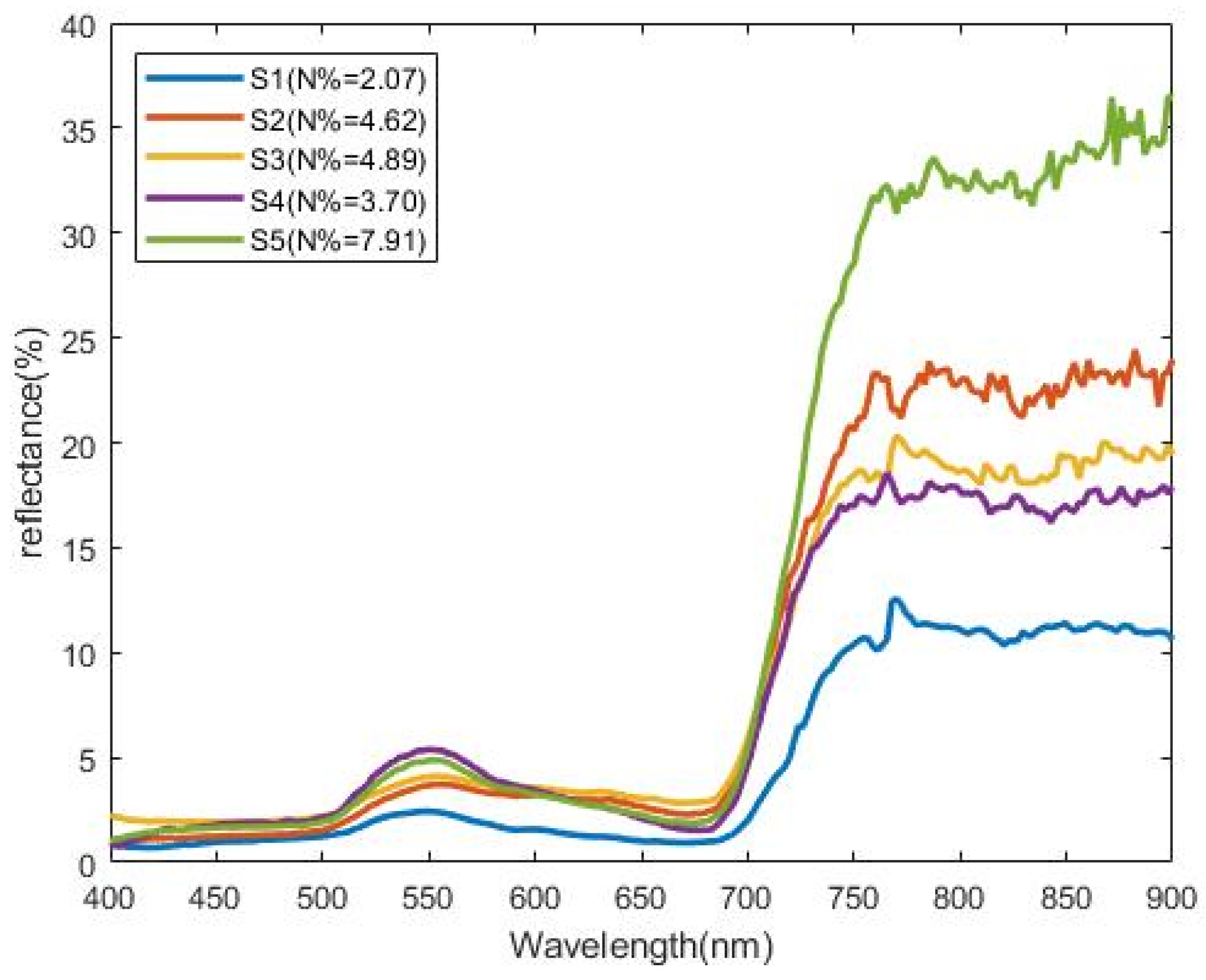
We have gathered the average emission spectra under various conditions as depicted in Figure 6. We have observed that the reflectance scenarios within the red-edge and near-infrared areas of the spectral curve vary under different nitrogen levels. In essence, the greater the nitrogen content, the more significant the variation in reflectance within the red-edge and near-infrared zones.

3.2. Hyperspectral Index Performance

According to

Table 4. Published predictions using hyperspectral indices.

	Bond			R2(50 samples)	R2(90 samples)
	Rλ1	Rλ2	Rλ3
NDVI	800	680		0.0029	0.1354
DVI	800	680		0.0534	0.4689
Vlopt	800	670		0.0537	0.5063
OSAVI	800	670		0.0001	0.1633
CIred-edge	780	710		0.0976	0.1403
RVI	800	670		0.0003	0.2768
MSAVI	810	670		0.0012	0.1636
SAVI	800	670		0.0001	0.1950
RDVI	800	670		0.0506	0.4560
mSR705	750	445	705	0.1035	0.2052
PSRI	680	500	750	0.0666	0.0251
TRSI	675	700	650	0.0978	0.1385
Bin2	498	413	442	0.0387	0.0708
Bin1	434	496	401	0.0659	0.0506
MCARI	700	670	550	0.0567	0.1140
MTCI	750	710	680	0.0950	0.1691
NDDA	755	680	705	0.0092	0.1967
mNDVIblue	924	703	423	0.0387	0.2283
Mrer	759	724	419	0.0996	0.0556
TVI	750	670	550	0.0284	0.4221
MTVI	800	550	670	0.0426	0.4216

, a linear regression model was established using chosen spectral indices, and all corresponding R-squared values were tabulated. In the set of experiments involving 50 samples, the selected HIs for nitrogen attributes yielded R-squared values all under 0.1, with an average R-squared at a mere 0.04. Meanwhile, in the set with 90 samples, the mean R-squared was still only 0.22. This indicates that the spectral indices currently available do not exhibit a strong correlation with the nitrogen content of the C. cathayensis Sarg canopy.

Optimized HIs were devised using various band combinations (

Table 5. Results of optimized hyperspectral index predictions.

	Bond						R250 samples	R290 samples
	Rλ1(50 samples)	Rλ2(50 samples)	Rλ3(50 samples)	Rλ1(90 samples)	Rλ2(90 samples)	Rλ3(90 samples)
Opt-NDVI	472	485		890	804		0.4939	0.6536
Opt-DVI	444	447		893	740		0.3416	0.6699
Opt-Vlopt	536	725		893	715		0.3787	0.6588
Opt-OSAVI	472	485		890	804		0.4864	0.6539
Opt-CI	472	485		919	532		0.5058	0.6882
Opt-RVI	473	486		919	532		0.5058	0.6882
Opt-MSAVI	485	472		930	549		0.4513	0.6760
Opt-SAVI	485	472		890	804		0.4697	0.6545
Opt-RDVI	444	447		893	785		0.4162	0.6725
Opt-mSR705	419	521	893	825	872	574	0.3815	0.7356
Opt-PSRI	734	738	485	675	596	927	0.5452	0.7563
Opt-TRSI	708	521	521	675	596	927	0.3489	0.4865
Opt-Bin2	604	630	610	774	893	800	0.5840	0.6948
Opt-Bin1	604	630	610	540	761	910	0.5495	0.7074
Opt-MCARI	434	440	432	910	766	872	0.4129	0.6902
Opt-MTCI	419	521	893	510	923	421	0.3815	0.7356
Opt-NDDA	559	539	543	923	425	510	0.9275	0.7356
Opt-mNDVI	517	921	708	847	889	910	0.9606	0.7187
Opt-Mrer	419	432	434	825	872	731	0.5122	0.7100
Opt-TVI	419	442	468	825	867	872	0.3453	0.6862
Opt-MTVI	419	442	485	825	867	872	0.2980	0.6868

) from the visible and near-infrared spectra (spanning from 400 to 930 nm), with the superior indices chosen based on sensitivity bands and R-squared values. We found that in certain optimized HIs, such as NDDA, the bands are very close to each other, indicating that this index can better capture the spectral features related to nitrogen concentration changes within this band range. Figure 7 illustrates two-dimensional contour plots and three-dimensional cross-sections of the optimized bi-band and tri-band HIs. The observed R-squared varied with the applied band combinations. The optimal HIs, the peak R-squared for canopy nitrogen concentration (CNC), and its sensitive wavelengths were deduced from these contour plots and cross-section diagrams. In the experiment comprising 50 samples, green (520–600 nm), blue (B, 450–500 nm), and near-infrared bands emerged as the sensitive, responsive bands according to the findings of opt-NDDA and opt-mNDVI (as showcased in Figure 8). Conversely, in the 90-sample experiment, the near-infrared band took center stage (as depicted in Figure 8), with the green, blue, and red-edge bands all rendering strong performances across a variety of indices.

The selection of optimal bands substantially improved the forecasting ability of the HIs (Figure 9). In comparison with established HIs, the R-squared improved from 2 to 92% in the 50-sample experiment and from 26 to 73% in the 90-sample experiment. Operating under analogous band optimization algorithms, the performance of optimized HIs varied. Besides the factors of band selection, HIs demonstrated different outcomes depending on the number of bands used. Furthermore, in contrast with dual-band indices, the triple-band indices significantly enhanced the predictions for CNC. On the whole, the accuracy of estimates from the optimized HIs with triple-band combinations outperformed those with dual-band combinations.

3.3. Evaluation of Optimal HIS, PLSR, and ML Method Performances

In this experiment, we used the reflectance values of hickory canopies as independent variables and constructed datasets with sample sizes of 50 and 90. A 10-fold cross-validation approach was employed to replace the traditional dataset division method. Machine learning algorithms such as PLSR, ANN, SVM, and RF were used to predict canopy nitrogen concentration. The number of latent variables in the PLSR model was set to two. For the ANN, a feedforward neural network was created with one hidden layer containing five neurons. The maximum number of training iterations was set to 20, and the learning rate was 0.01. In the RF model, the number of trees was set to 40. For the SVM, the radial basis function (RBF) was selected as the kernel function, and the kernel scale was automatically adjusted using the KernelScale function.

The predictive models for the growth period of C. cathayensis Sarg pulp are summarized in the table below (

Table 6. Fit results from various models.

	Calibration (Cross-Validated)			Validation
Method	R2	RMSE	RE	R2	RMSE	RE
NDDA	0.92	1.02	0.23	0.96	1.05	0.24
mNDVI	0.96	0.71	0.16	0.98	0.82	0.19
PLSR50	0.18	3.25	0.42	0.27	0.85	0.52
RF50	0.61	2.42	2.09	0.54	2.37	2.40
ANN50	0.50	2.55	0.39	0.47	0.19	0.08
SVM50	0.73	1.83	5.70	0.77	1.756	6.92
PLSR90	0.63	2.59	0.79	0.71	2.30	0.84
RF90	0.62	2.65	0.59	0.61	3.32	1.05
ANN90	0.75	2.11	0.31	0.68	2.39	0.21
SVM90	0.67	5.19	10.73	0.66	5.18	10.87

). During this stage, the SVM model achieves the highest R², reaching 0.73, surpassing even the optimal HIs When compared with models based on the optimal HIS, PLSR and ML methods do not exhibit distinct advantages. Furthermore, the optimal HIS model shows lower RE and RMSE, coupled with a higher R². These findings suggest that, within a specific growth cycle, modeling based on optimized HIS provides better predictive performance.

3.4. Evaluation of Optimized Hyperspectral Indices

Analysis results reveal substantial differences among various opt-HIs, particularly evident in sensitivity analysis where NE values tend to vary significantly among different HIs. Moreover, in stability analysis, the CV of most optimized HIs exhibits considerable fluctuations with the increasing chlorophyll content. The results indicate that the predictive capacity of optimized HIs is determined by both the selection of spectral bands and the architectural composition of the HIs’ formulas.

By comparing the NE values (

Table 7. Analysis of sensitivity.

NDVI (2bond)	DVI (2bond)	VIopt (2bond)	OSAVI (2bond)	CI (2bond)	RVI (2bond)	MSAVI (2bond)	SAVI (2bond)	RDVI (2bond)
0.010	0.054	0.494	0.011	0.020	0.020	0.016	0.013	0.033
PSRI	Bin2	Bin1	MTCI	NDDA	mNDVI	Mrer	TVI	MTVI
0.300	0.029	0.008	4.822	256.386	1.010	0.060	3.854	0.170

), it is evident that certain indices among the tri-band HIs have lower NE values than most of the dual-band indices, indicating that tri-band HIs may exhibit better sensitivity and stability in predicting CNC. Additionally, through the analysis of CV stability (

Table 8. The coefficient of variation (CV) of optimized spectral indices for different chlorophyll content.

LCC	RVI	CIred-edge	NDVI	SAVI	OSAVI	NDDA	mNDVIblue	PSRI	mSR705
10	0.33	18.80	18.92	9.54	11.58	12.12	6.83	6.12	15.38
20	0.12	17.05	17.09	5.88	8.21	12.17	4.72	7.39	15.42
30	0.05	67.26	67.26	72.09	70.79	12.11	4.02	8.10	15.55
40	0.17	28.04	27.99	18.54	20.44	12.01	3.70	8.52	15.76
50	0.24	26.08	26.00	15.83	17.88	11.66	3.54	8.47	16.08
60	0.28	25.42	25.32	14.88	16.98	12.22	3.45	9.43	16.53

), most tri-band HIs demonstrate lower CV values with less variation, suggesting that tri-band HIs are better equipped to handle variability across different datasets, thereby providing more stable predictive performance.

4. Discussion

4.1. Characteristic Analysis of Spectral Data

As delineated in Figure 5, the canopy spectral curves of hickory trees across diverse regions demonstrate a distinct separation and lack of overlap as nitrogen content varies, with the red-edge region being particularly indicative. This region is affirmed as advantageous for monitoring plant nitrogen [41], and its efficacy and accuracy in estimating chlorophyll, total nitrogen, and yield are well substantiated. Likewise, the near-infrared band exhibits analogous tendencies, with spectral reflectance variations closely tied to the nitrogen content. Typically, shifts in plant near-infrared spectral behavior correlate with the structural organization of mesophyll cellular molecules [42], and reflectance discrepancies serve as indicators of leaf nutritional status, tending to amplify with improved nutrition. Leaf structural traits evolve in tandem with nitrogen content: greater nitrogen engenders an expanded leaf surface area. Concurrently, the leaf epidermis thickens, mesophyll cell dimensions increase, and their arrangement becomes denser, which in turn augments chlorophyll levels. This thickening of epidermal tissue facilitates active gas exchange, thus bolstering photosynthesis. These findings are corroborated by the literature [43]. However, such a phenomenon was not observed in the canopy spectral curves of hickory with similar nitrogen levels (as in curves S2, S3, and S4 of Figure 6), which is attributed to nutritional or moisture imbalances [44]. These outcomes underscore the significance of the near-infrared band in forecasting hickory’s nitrogen content, with both near-infrared and red-edge bands being crucial in evaluating plant nitrogen nutrition.

4.2. Refinement of HIS

The improvement of hyperspectral indices in this study proceeded based on optimal band combinations, examining all conceivable band pairings within the 400–930 nm range. The sensitive band for hickory cnc was determined by analyzing the pattern of these band combinations. Current results suggest the reactive bands for hickory canopy primarily reside in the blue light section of the visible spectrum (450–520 nm), the green light region (520–600 nm), the red-edge region (690–750 nm), and the near-infrared brigades (750–930 nm). It should be noted that simply zoning in on the combination with the best R² value was deemed insufficient. Hence, in experiments incorporating larger sample sizes, outcomes with R² values above 0.6 were included. It was ascertained that the blue and green light regions of the visible spectrum, along with the near-infrared zone, played a pivotal role in predicting hickory canopy nitrogen content. The near-infrared band demonstrated its crucial function in hickory cnc forecasts by featuring in all band combinations. Summarily, near-infrared proved to be the highest-performing band for hickory nitrogen estimation, with the red-edge, green light, and blue light sectors attaining commendable results in several optimized indices. This is ascribed to significant differences in canopy structures throughout hickory’s growth cycle [24], stirring a shift in hickory cnc’s responsive bands towards shorter wavelengths.

4.3. Impact of Growth Stages on the Performance of Models Estimating Nitrogen Traits in C. cathayensis Sarg

The performance of several hyperspectral indices (HIs) in estimating plant nitrogen concentration (PNC) in irrigated perennial ryegrass was evaluated in a study [45]. The study found that these chosen HIs exhibited substantial correlation when applied to data from a singular growth period. Our research focuses on hickory trees and reveals that models that optimize HIs show superior performance in predicting singular growth stages. However, in the context of experiments involving mixed growth stages, the prediction efficacy of the optimized HIs—specifically, the exceedingly optimal opt-mndvi and opt-ndda—noticeably decreased, yet still maintained a relatively high level (R² > 0.7). Furthermore, the projection results using machine learning methods showed an increasing trend.

Our findings suggest that for stage-specific models, the PLSR and ML models often perform similarly to, if not worse than, corresponding HIS-based models. This underscores that for stage-specific models, HIS-based estimations are the pinnacle of performance and have no room for additional improvement. On the other hand, the improvement in ML model performance highlights its potential for predictions spanning the entire growth period of hickory trees. We acknowledge the limitations of our study, such as the lack of completeness in the growth cycle for sample collection and the scarcity of collected samples. To mitigate this, we are committed to systematically augmenting our experimental data in future studies.

4.4. The Influence of the Optimization Algorithm Applied to HIs on the Precision of Predicting CNC

Our research ascertained that pinpointing the optimal spectral band combinations for hyperspectral indices (HIs) can notably enhance the accuracy of estimating canopy nitrogen concentration (CNC) in hickory trees, echoing findings from prior studies on crops like wheat [46] and rice [30]. Nonetheless, the influence of different HI algorithmic formulations on prediction efficacy must be acknowledged. Consequently, our study looked into how various formulaic structures of hyperspectral indices contribute to the band optimization’s estimation capabilities. The findings suggest that band optimization can partially mitigate the effects of certain HI formulaic structures, exemplified by indices such as Opt-NDDA, Opt-mSR705, Opt-mND705, and Opt-mTVI. Appropriate formulaic structures of hyperspectral indices can further refine HIs’ proficiency in CNC extraction, thus elevating the precision of estimations. These insights emphasize the significance of strategic band selection and index formula structuring within the realm of hyperspectral remote sensing to improve the monitoring and predictive assessment of vegetative health. Moreover, preceding research [47] has indicated that three-band HIs offer greater stability in estimating vegetation nitrogen content over their two-band counterparts. Our findings corroborate that the integration of a third band into two-band indices considerably augments the predictive power of HIs. The applicability of this enhancement extends to forecasting within economic forestry contexts as well.

4.5. Evaluation of Optimized HIs

Beyond utilizing R² as the statistical hallmark of our models, our research delved into NE analysis to discern the optimized HIs’ sensitivity in CNC estimations. By leveraging the PROSAIL model for CV computation, we aimed to ascertain the HIs’ performance stability, coupled with employing cross-validation datasets from our experimental plots to gauge HIS accuracy. Notably, in juxtaposing opt-NDDA and opt-mNDVI—each boasting R² values beyond 0.9—opt-mNDVI emerged as the superior predictor of hickory nitrogen content, courtesy of its lower NE and modestly lesser CV values. This revelation underscores that the predominance of a singular metric should not dictate the optimum HIS determination. Pertinently, for singular growth phase inquiries, the optimal HIs for precise hickory CNC determination stood as (R₅₁₇ − R₉₂₃ + 2 × R₇₀₈)/(R₅₁₇ + R₉₂₃ – 2 × R₇₀₈) (opt-mNDVI), each registering correlation coefficients above 0.9 with hickory CNC. Meanwhile, in mixed-growth-phase examinations, opt-psri, opt-mSR705, opt-NDDA, and opt-mNDVI showcased commendable efficacy.

Our investigation employed an integrative index to critically assess and refine the optimized HIs, paving the way for their enhanced applicability. Moreover, our study’s knack for pinpointing specific wavelengths while upholding utmost accuracy provides a dual benefit of curtailing operational costs and access hurdles, all the while safeguarding meticulous monitoring prowess. This duality significantly bolsters the advancement and pragmatic application of precision agriculture.

5. Conclusions

Low-altitude drone data collection is notably prone to interference from a myriad of external factors. The process of canopy spectral extraction from hyperspectral imagery serves as a critical step in mitigating noise within spectral data and diminishing the influence of soil reflectivity on canopy reflectance, underscoring the necessity of canopy extraction in the preprocessing of hyperspectral images. In the realm of UAV-based hyperspectral imaging for hickory canopy nitrogen concentration surveillance, diverse modeling approaches yield distinct outcomes. Models predicated on optimized HIs exhibit superior efficacy within certain growth stages, while methodologies such as PLSR, ANN, RF, and SVM lag in predictive accuracy during specific phases, yet their performance is enhanced throughout the entire growth cycle. In pursuit of advancing optimized HIS for hickory CNC prediction, our study engaged with 23 HI formulas, conducting empirical analyses across various hickory experimental sites. It became evident that HIs’ effectiveness in CNC estimation is significantly swayed by both formulaic structures and spectral band optimization. We postulate that the ideal HIS formula may vary across different growth stages, warranting further inquiry. In the quest for the most fitting HIS, sensitive spectral bands for the hickory canopy encompass visible wavelengths inclusive of green and blue light, along with the red-edge and near-infrared bands. Opt-mNDVI emerged as the most proficient index in terms of sensitivity, accuracy, and stability for CNC estimations across varying locales, moisture levels, and nitrogen applications. These insights affirm that crafting an optimized HI linear regression model remains a sound strategy for the assessment of hickory canopy nitrogen concentration, with the selection of the most suitable HIS being of paramount importance to predictive accuracy. Our findings aim to guide the establishment of standardized HIs, thereby enabling precise CNC estimations for economic forests on a grander scale.

This study utilized drone-based hyperspectral imaging technology to accurately evaluate CNC. Through the optimization of band combinations and HI formulas, the predictive capacity of the HIs was significantly enhanced, particularly under complex field conditions. The findings indicated that the optimized HIs achieved the highest predictive accuracy during a single growth stage, with an R² of 0.96 and an RMSE of 0.71. For the entire growth cycle, the R² was 0.75 and the RMSE was 2.11, demonstrating robust predictive performance across different growth stages. The optimization of band combinations improved the predictive performance of the HIs by 16% to 71%, with three-band combinations outperforming two-band combinations by 4% to 46%. By integrating optimized HIs with machine learning algorithms, the method proved applicable across various locations, moisture levels, and nitrogen application conditions, providing stable predictions even under complex field environments, thus exhibiting strong practical value. The conclusions of this study provide a foundation for the establishment of standardized HIs, thereby supporting large-scale, precise nitrogen concentration monitoring and nitrogen management in economic forests. However, further validation is needed to assess the applicability of this method to other hickory varieties and different crops. Future research should extend this approach to a broader range of targets and species to enhance nitrogen concentration monitoring in economic forestry.

References

1. Yan, F.; Wang, Q.; Teng, J.; Wu, F.; He, Z. Preparation process optimization and evaluation of bioactive peptides from Carya cathayensis Sarg meal. Curr. Res. Food Sci. 2023, 6, 100408. [Google Scholar] [CrossRef]
2. Yang, J.; Zhou, F.; Xiong, L.; Mao, S.; Hu, Y.; Lu, B. Comparison of phenolic compounds, tocopherols, phytosterols and antioxidant potential in Zhejiang pecan [Carya cathayensis] at different stir-frying steps. LWT Food Sci. Technol. 2015, 62, 541–548. [Google Scholar] [CrossRef]
3. Sáez-Plaza, P.; Michalowski, T.; Navas, M.J.; Asuero, A.G.; Wybraniec, S. An overview of the Kjeldahl method of nitrogen determination. Part I. Early History, chemistry of the procedure, and titrimetric finish. Crit. Rev. Anal. Chem. 2013, 43, 178–223. [Google Scholar] [CrossRef]
4. Sáez-Plaza, P.; Navas, M.J.; Wybraniec, S.; Michalowski, T.; Asuero, A.G. An overview of the Kjeldahl method of nitrogen determination. Part II. Sample preparation, working scale, instrumental finish, and quality control. Crit. Rev. Anal. Chem. 2013, 43, 224–272. [Google Scholar] [CrossRef]
5. Wang, X.X.; Cai, G.S.; Lu, X.P.; Yang, Z.N.; Zhang, X.J.; Zhang, Q.G. Inversion of Wheat Leaf Area Index by Multivariate Red-Edge Spectral Vegetation Index. Sustainability 2022, 14, 15875. [Google Scholar] [CrossRef]
6. Wu, B.; Zheng, H.; Xu, Z.L.; Wu, Z.W.; Zhao, Y.D. Forest Burned Area Detection Using a Novel Spectral Index Based on Multi-Objective Optimization. Forests 2022, 13, 1787. [Google Scholar] [CrossRef]
7. Huerta, R.F.M.; Gonzalez, R.G.G.; Medina, L.M.C.; Pacheco, I.; Olivarez, J.P.; Velazquez, R.V. A review of methods for sensing the nitrogen status in plants: Advantages, disadvantages and recent advances. Sensors 2013, 13, 10823–10843. [Google Scholar] [CrossRef]
8. Qian, S.-E. Hyperspectral satellites, evolution, and development history. IEEE J. Sel. Top. Appl. Earth Obs. Remote Sens. 2021, 14, 7032–7056. [Google Scholar] [CrossRef]
9. Guelman, M.; Ortenberg, F. Small satellite’s role in future hyperspectral Earth observation missions. Acta Astronaut. 2009, 64, 1252–1263. [Google Scholar] [CrossRef]
10. Vangi, E.; D’Amico, G.; Francini, S.; Giannetti, F.; Lasserre, B.; Marchetti, M.; Chirici, G. The new hyperspectral satellite PRISMA: Imagery for forest types discrimination. Sensors 2021, 21, 1182. [Google Scholar] [CrossRef]
11. Osco, L.P.; Ramos, A.P.M.; Moriya, É.A.S.; de Souza, M.; Marcato, J., Jr.; Matsubara, E.T.; Imai, N.N.; Creste, J.E. Improvement of leaf nitrogen content inference in Valencia-orange trees applying spectral analysis algorithms in UAV mounted-sensor images. Int. J. Appl. Earth Obs. Geoinf. 2019, 83, 101907. [Google Scholar] [CrossRef]
12. Xu, L.; Lu, C.; Zhou, T.; Wu, J.; Feng, H. A 3D-2DCNN-CA approach for enhanced classification of hickory tree species using UAV-based hyperspectral imaging. Microchem. J. 2024, 199, 109981. [Google Scholar] [CrossRef]
13. Guo, P.; Li, M.; Luo, W.; Cha, Z. Estimation of foliar nitrogen of rubber trees using hyperspectral reflectance with feature bands. Infrared Phys. Technol. 2019, 102, 103021. [Google Scholar] [CrossRef]
14. Perry, E.M.; Goodwin, I.; Cornwall, D. Remote sensing using canopy and leaf reflectance for estimating nitrogen status in red-blush pears. HortScience 2018, 53, 78–83. [Google Scholar] [CrossRef]
15. Davenport, J.R.; Stevens, R.G.; Perry, E.M.; Lang, N.S. Leaf spectral reflectance for nondestructive measurement of plant nutrient status. HortTechnology 2005, 15, 31–35. [Google Scholar] [CrossRef]
16. Rouse, J.W.; Haas, R.H.; Deering, D.W.; Schell, J.A.; Harlan, J.C. Monitoring the Vernal Advancement and Retrogradation (Green Wave Effect) of Natural Vegetation; NASA/GSFC Type III Final Report; NASA: Greenbelt, MD, USA, 1974; p. 371.
17. Huete, A. A soil-adjusted vegetation index (SAVI). Remote Sens. Environ. 1988, 25, 295–309. [Google Scholar] [CrossRef]
18. Qi, J.; Chehbouni, A.; Huete, A.R.; Kerr, Y.H.; Sorooshian, S. A modified soil adjusted vegetation index. Remote Sens. Environ. 1994, 48, 119–126. [Google Scholar] [CrossRef]
19. Rondeaux, G.; Steven, M.; Baret, F. Optimization of soil-adjusted vegetation indices. Remote Sens. Environ. 1996, 55, 95–107. [Google Scholar] [CrossRef]
20. Li, F.; Miao, Y.; Hennig, S.D.; Gnyp, M.L.; Chen, X.; Jia, L.; Bareth, G. Evaluating hyperspectral vegetation indices for estimating nitrogen concentration of winter wheat at different growth stages. Precis. Agric. 2010, 11, 335–357. [Google Scholar] [CrossRef]
21. Adão, T.; Hruška, J.; Pádua, L.; Bessa, J.; Peres, E.; Morais, R.; Sousa, J.J. Hyperspectral imaging: A review on UAV-based sensors, data processing and applications for agriculture and forestry. Remote Sens. 2017, 9, 1110. [Google Scholar] [CrossRef]
22. Verrelst, J.; Malenovský, Z.; Van der Tol, C.; Camps-Valls, G.; Gastellu-Etchegorry, J.P.; Lewis, P.; North, P.; Moreno, J. Quantifying vegetation biophysical variables from imaging spectroscopy data: A review on retrieval methods. Surv. Geophys. 2019, 40, 589–629. [Google Scholar] [CrossRef] [PubMed]
23. Thenkabail, P.S.; Smith, R.B.; De Pauw, E. Hyperspectral vegetation indices and their relationships with agricultural crop characteristics. Remote Sens. Environ. 2000, 71, 158–182. [Google Scholar] [CrossRef]
24. Yang, H.; Li, F.; Hu, Y.; Yu, K. Hyperspectral indices optimization algorithms for estimating canopy nitrogen concentration in potato (Solanum tuberosum L.). Int. J. Appl. Earth Obs. Geoinf. 2021, 102, 102416. [Google Scholar] [CrossRef]
25. Gitelson, A.A.; Gritz, Y.; Merzlyak, M.N. Relationships between leaf chlorophyll content and spectral reflectance and algorithms for non-destructive chlorophyll assessment in higher plant leaves. J. Plant Physiol. 2003, 160, 271–282. [Google Scholar] [CrossRef]
26. Tucker, C.J. Red and photographic infrared linear combinations for monitoring vegetation. Remote Sens. Environ. 1979, 8, 127–150. [Google Scholar] [CrossRef]
27. Gonenc, A.; Ozerdem, M.S.; Emrullah, A.C. Comparison of NDVI and RVI vegetation indices using satellite images. In Proceedings of the 2019 8th International Conference on Agro-Geoinformatics (Agro-Geoinformatics), Istanbul, Turkey, 16–19 July 2019. [Google Scholar]
28. Melillos, G.; Themistocleous, K.; Hadjimitsis, D.G. Detecting underground structures in vegetation indices: MSR, RDVI, OSAVI, IRG, time series using histograms. In Proceedings of the Eighth International Conference on Remote Sensing and Geoinformation of the Environment (RSCy2020), Paphos, Cyprus, 16–18 March 2020; Volume 11524, pp. 617–623. [Google Scholar]
29. Reyniers, M.; Walvoort, D.J.; De Baardemaaker, J. A linear model to predict with a multi-spectral radiometer the amount of nitrogen in winter wheat. Int. J. Remote Sens. 2006, 27, 4159–4179. [Google Scholar] [CrossRef]
30. Tian, Y.; Yao, X.; Yang, J.; Cao, W.; Hannaway, D.B.; Zhu, Y. Assessing newly developed and published vegetation indices for estimating rice leaf nitrogen concentration with ground- and space-based hyperspectral reflectance. Field Crops Res. 2011, 120, 299–310. [Google Scholar] [CrossRef]
31. Sims, D.A.; Gamon, J.A. Relationships between leaf pigment content and spectral reflectance across a wide range of species, leaf structures and developmental stages. Remote Sens. Environ. 2002, 81, 337–354. [Google Scholar] [CrossRef]
32. Wang, W.; Yao, X.; Yao, X.; Tian, Y.; Liu, X.; Ni, J.; Cao, W.; Zhu, Y. Estimating leaf nitrogen concentration with three-band vegetation indices in rice and wheat. Field Crops Res. 2012, 129, 90–98. [Google Scholar] [CrossRef]
33. Feng, W.; Guo, B.; Zhang, H.; He, L.; Zhang, Y.; Wang, Y.; Zhu, Y.; Guo, T. Remote estimation of above ground nitrogen uptake during vegetative growth in winter wheat using hyperspectral red-edge ratio data. Field Crops Res. 2015, 180, 197–206. [Google Scholar] [CrossRef]
34. Dash, J.; Curran, P.J. The MERIS terrestrial chlorophyll index. Int. J. Remote Sens. 2004, 25, 5403–5413. [Google Scholar] [CrossRef]
35. Haboudane, D.; Miller, J.R.; Pattey, E.; Zarco-Tejada, P.J.; Strachan, I.B. Hyperspectral vegetation indices and novel algorithms for predicting green LAI of crop canopies: Modeling and validation in the context of precision agriculture. Remote Sens. Environ. 2004, 90, 337–352. [Google Scholar] [CrossRef]
36. Daughtry, C.S.T.; Walthall, C.L.; Kim, M.S.; De Colstoun, E.B.; McMurtrey, J.E., III. Estimating corn leaf chlorophyll concentration from leaf and canopy reflectance. Remote Sens. Environ. 2000, 74, 229–239. [Google Scholar] [CrossRef]
37. Feng, W.; Guo, B.; Wang, Z.; He, L.; Song, X.; Wang, Y.; Guo, T.C. Measuring leaf nitrogen concentration in winter wheat using double-peak spectral reflection remote sensing data. Field Crops Res. 2014, 159, 43–52. [Google Scholar] [CrossRef]
38. Merzlyak, M.N.; Gitelson, A.A.; Chivkunova, O.B.; Rakitin, V.Y. Non-destructive optical detection of pigment changes during leaf senescence and fruit ripening. Physiol. Plant. 1999, 106, 135–141. [Google Scholar] [CrossRef]
39. Chappelle, E.W.; Kim, M.S.; McMurtrey, J.E., III. Ratio analysis of reflectance spectra (RARS): An algorithm for the remote estimation of the concentrations of chlorophyll a, chlorophyll b, and carotenoids in soybean leaves. Remote Sens. Environ. 1992, 39, 239–247. [Google Scholar] [CrossRef]
40. Broge, N.H.; Leblanc, E. Comparing prediction power and stability of broadband and hyperspectral vegetation indices for estimation of green leaf area index and canopy chlorophyll density. Remote Sens. Environ. 2001, 76, 156–172. [Google Scholar] [CrossRef]
41. Atzberger, C.; Guerif, M.; Baret, F.; Werner, W. Comparative analysis of three chemometric techniques for the spectroradiometric assessment of canopy chlorophyll content in winter wheat. Comp. Elecron. Agric. 2010, 73, 165–173. [Google Scholar] [CrossRef]
42. Yanli, L.; Qiang, L.; Shaolan, H.; Shilai, Y.; Xuefeng, L.; Rangjin, X.; Youngqiang, Z.; Lie, D. Prediction of nitrogen and phosphorus contents in citrus leaves based on hyperspectral imaging. Int. J. Agric. Biol. Eng. 2015, 8, 80–88. [Google Scholar] [CrossRef]
43. Min, M.; Lee, W. Determination of significant wavelengths and prediction of ni-trogen content for citrus. Am. Soc. Agric. Eng. 2005, 48, 455–461. [Google Scholar] [CrossRef]
44. O’Connell, J.L.; Byrd, K.B.; Kelly, M. Remotely-sensed indicators of N-related biomass allocation in Schoenoplectus acutus. PLoS ONE 2014, 9, e90870. [Google Scholar] [CrossRef] [PubMed]
45. Patel, M.K.; Ryu, D.; Western, A.W.; Fitzgerald, G.J.; Perry, E.M.; Suter, H.; Young, I.M. A new multispectral index for canopy nitrogen concentration applicable across growth stages in ryegrass and barley. Precis. Agric. 2024, 25, 486–519. [Google Scholar] [CrossRef]
46. Li, F.; Mistele, B.; Hu, Y.C.; Chen, X.P.; Schmidhalter, U. Optimising three-band spectral indices to assess aerial N concentration, N uptake and aboveground biomass of winter wheat remotely in China and Germany. ISPRS J. Photogramm. Remote Sens. 2014, 92, 112–123. [Google Scholar] [CrossRef]
47. Dian, Y.; Le, Y.; Fang, S.; Xu, Y.; Yao, C.; Liu, G. Influence of spectral bandwidth and position on chlorophyll content retrieval at leaf and canopy levels. J. Indian Soc. Remote Sens. 2016, 44, 583–593. [Google Scholar] [CrossRef]
Figure 1. The experimental area.
Remotesensing 16 03780 g001
Figure 2. Workflow diagram illustrating the methodology of this study.
Remotesensing 16 03780 g002
Figure 3. Nitrogen concentration in C. cathayensis Sarg trees at different locations: S1—Xigu Ping during the fruiting period in 2022; S2—Sengui Tang during the same period; S3—Qingliang Feng also during the fruiting period of 2022; S4—Taihu Source at the end of dormancy in 2023; and S5—Taihu Source during the fruit expansion period in 2023. The nitrogen concentration distribution is portrayed through box plots where each box corresponds to a dataset (S1, S2, S3, S4, S5). The box itself highlights the 25th and 75th percentiles of each dataset, signifying that the box’s bottom and top represent the lower quartile (Q1) and upper quartile (Q3), respectively. The whiskers stretch from the 10th to the 90th percentiles, offering a view of the range of data distribution but excluding the outliers. The median (50th percentile) of each dataset is depicted by a line within the box and is typically noted numerically above the box plot. “+” signs mark the outliers in nitrogen concentration.
Remotesensing 16 03780 g003
Figure 4. Process of canopy extraction: (a) hyperspectral image, (b) NDVI calculation, (c) mask extraction, (d) smooth processing, and (e) extract results.
Remotesensing 16 03780 g004
Figure 5. (a) The reflectance spectra for 50 samples. (b) The mean reflectance spectrum of the 50 samples. (c) The reflectance spectra for 90 samples. (d) The mean reflectance spectrum of the 90 samples.
Remotesensing 16 03780 g005
Figure 6. Average reflectance spectra under varying conditions: S1: Xiguaping (phase of fruit drop in 2022); S2: Sen’guitang (phase of fruit drop in 2022); S3: Qingliangfeng (phase of fruit drop in 2022); S4: Taihu Lake Source (end of dormancy in 2023); S5: Taihu Lake Source (period of fruit enlarging in 2023). N% denotes the mean nitrogen concentration pertaining to the conditions of the given area.
Remotesensing 16 03780 g006
Figure 7. Combinations of three bands among the 50 samples: (a) mNDVI and (b) NDDA. Combinations of two bands among the 90 samples: (c) NDVI, (d) CI, and (e) MSAVI. Combinations of three bands among the 90 samples: (f) mNDVI, (g) MTCI, and (h) NDDA.
Remotesensing 16 03780 g007
Figure 8. Sensitivity band statistics for NDDA and mNDVI (50 samples): (a) opt-mNDVI and (b) opt-NDDA. Frequency of sensitive bands (90 samples): violet (V) spans 400–450 nm, blue (B) spans 450–520 nm, green (G) spans 520–600 nm, red (R) spans 600–690 nm, red-edge (RE) spans 690–760 nm, and near-infrared (NIR) spans 750–1050 nm. (c) opt-NDVI, (d) opt-DVI, (e) opt-MSAVI, (f) opt-mSR705, (g) opt-PSRI, (h) opt-BIN1, (i) opt-BIN2, (j) opt-mNDVI, and (k) opt-MCARI.
Remotesensing 16 03780 g008
Figure 9. Comparative analysis of the prediction ability of optimized spectral index models for C. cathayensis Sarg canopy nitrogen concentration. (a): R2 of prediction results for different optimized spectral indices, (b): RMSE of prediction results for different optimized spectral indices, (c): RE of prediction results for different optimized spectral indices.
Remotesensing 16 03780 g009