Abstract
The potential of satellite soil moisture (SM) in improving hydrological modeling has been addressed in synthetic experiments, but it is less explored in real data cases. Here, we investigate the added value of Soil Moisture and Passive (SMAP) and Advanced Scatterometer (ASCAT) SM data to distributed hydrological modeling with the soil and water assessment tool (SWAT) in a highly human disturbed catchment (126, 486 km2) featuring a network of SM and streamflow observations. The investigation is based on the ensemble Kalman filter (EnKF) considering SM errors from satellite data using the triple collocation. The assimilation of SMAP and ASCAT SM improved the surface (0–10 cm) and rootzone (10–30 cm) SM at >70% and > 50% stations of the basin, respectively. However, the assimilation effects on distributed streamflow simulation of the basin are un-significant and not robust. SM assimilation improved the simulated streamflow at two upstream stations, while it deteriorated the streamflow at the remaining stations. This can be largely attributed to the poor vertical soil water coupling of SWAT, suboptimal model parameters, satellite SM data quality, humid climate, and human disturbance to rainfall-runoff processes. This study offers strong evidence of integrating satellite SM into hydrological modeling in improving SM estimation and provides implications for achieving the added value of remotely sensed SM in streamflow improvement.
1. Introduction
Soil moisture (SM) plays a crucial role in the energy and water cycle between land and atmosphere [1]. It not only exerts a strong control on the partitioning of incoming radiation into latent and sensible heat fluxes, but also determines the partitioning of precipitation into surface runoff and infiltration [2,3]. In hydrological modeling, rainfall-runoff processes in a catchment are largely controlled by the initial state of SM [4]. Thus, an accurate SM estimation is deemed to have great potential to improve hydrological simulation and prediction within a catchment [5].
The integration of SM observations in hydrological modeling via data assimilation (DA) techniques is considered a promising approach to improve SM estimation and rainfall-runoff modeling [6,7,8,9]. DA techniques provide an integrated framework to analyze all sources of uncertainties from modeling and observation, including the errors of model forcing inputs, model parameters, and model structures, as well as the observation errors from in situ measurements and remote sensing [10]. The assimilation of high-quality in situ SM data in hydrological modeling has been proven to benefit the SM and streamflow estimation [11,12,13]. Nevertheless, the benefits are limited by sparse field measurement sites with lacking capacity to fully account for the spatial heterogeneity of SM.
Remote sensing provides large-scale spatially and temporally continuous SM data. The ever-improving observation and retrieval techniques and thereby data quality have largely promoted remote sensing applications in DA in recent decades [14,15,16,17,18,19,20]. Currently, the potential of remote sensing SM assimilation on the improvement in SM and runoff estimation in hydrological modeling has been validated in synthetic experiments [21,22,23,24,25,26]. However, the performance of real DA remains largely unexplored. There is still no consensus on the efficacy of remotely sensed SM for hydrological simulation and prediction. Brocca et al. [27] assimilated the Advanced Scatterometer (ASCAT) SM and the Advanced Microwave Scanning Radiometer for Earth observations (AMSR-E) SM into a distributed rainfall-runoff model (MISDc) in six basins of Italy, Luxembourg, France, and the US. They found a general positive impact on runoff prediction, but no improvement in mountainous and snow-dominated regions. Alvarez-Garreton et al. [16] improved hydrological prediction in a semiarid catchment by assimilating the AMSR-E SM into a probability distributed model. Similar conclusions were obtained by Lievens et al. [17] who assimilated the Soil Moisture Ocean Salinity (SMOS) SM into the Variable Infiltration Capacity (VIC) model over the Murray Darling basin, Australia. Corato et al. [28] found that the DA performance of remotely sensed SM was vegetation and time dependent for a catchment in the UK, whereas Nayak et al. [29] underscored the significance of model structure in the DA performance. Massari et al. [30] demonstrated that the remote sensing SM data quality and the accurate model and observation error assumption and estimation have a significant impact on the assimilation results. In view of the current unknown modelling and observation error, the immature model structure, and the varying data quality of satellite SM, the efficacy of remote sensing SM DA in hydrological modeling requires further investigation [31,32,33].
This study investigated the impact of the Soil Moisture Active and Passive (SMAP) and the ASCAT SM DA on the distributed hydrological simulation with the soil and water assessment tool (SWAT) model in a watershed highly disturbed by human activities in China. The selection of the SWAT model considers its wide applicability in catchment hydrological modeling and the unexplored performance of satellite SM retrievals [8,21,23]. The investigation is based on a robust data assimilation approach of the ensemble Kalman filter (EnKF), considering the observation errors based on the triple collocation (TC) method. Our focus is on the impact of the remotely sensed surface SM DA on profile SM and streamflow estimation in SWAT for a highly disturbed catchment.
2. Methodology
2.1. SWAT Model
SWAT is a physically based basin scale distributed model, widely used to predict the impacts of land management practices on water, sediment, and agricultural chemical yields in large, complex catchments with varying land use, soil, and topography over long periods of time [34]. For modeling purposes, a catchment is geographically partitioned into a number of sub-catchments or subbasins; then, each subbasin is further divided into several Hydrological Response Units (HRUs) with unique land cover, soil type, and slope steepness. HRUs are the basic units for land phase of hydrological cycle modeling including surface runoff generation, evapotranspiration, soil water routing, and groundwater generation. SM plays a critical role in the rainfall-runoff process. SM modulates the redistribution of water infiltrated or percolated to the soil profile, which can largely impact evapotranspiration, surface runoff, and groundwater generation directly or indirectly, and finally river flow through overland and channel flow concentration. The water balance equation for each soil layer is as follows:
where SWt−1,ly and SWt,ly are the soil water content (mm) at the start and end of the day for layer ly; ∆wperc,ly is the net water percolation received in layer ly; Qlat,ly is the lateral flow generated from layer ly; and Ea,ly is the evapotranspiration drawn from layer ly.
The vertical movement of soil water in unsaturated soil layers is dominated by the evapotranspiration process. Potential evapotranspiration (PET) is first calculated with the Penman-Monteith equation [35]. The potential soil water evaporation is a function of PET and leaf area index, and the potential plant uptake can also be estimated from the Penman-Monteith equation. The total potential soil water evaporation and plant uptake is allocated to each soil layer with the depth distribution function. The actual soil water extraction is constrained by the available soil water of a given layer and not allowed to be compensated from another layer. This deficiency is made up by a soil and a plant compensation factor to adjust the depth distribution of the potential soil water evaporation and ideal plant uptake.
2.2. The Ensemble Kalman Ffilter (EnKF)
The ensemble Kalman filter (EnKF) is proposed based on the theory of the linear Kalman filter by incorporating the Monte Carlo method to generate a state ensemble representing the probability distribution of the state, for example SM [36,37]. The predicted state ensemble at time t is given by the following:
where F indicates the SWAT model; represents the updated state ensemble at time t − 1. In this study, includes the three-layer profile SM for each subbasin (Table 1). It indicates the model forcing inputs (e.g., precipitation and temperature) at time t. μt is the stochastic perturbation of the forecast state and represents the modeling error, assumed to have a normal distribution with zero mean and a variance of δ2. The state update of is obtained by the following:
where Yt is the observation ensemble at time t, which is generated by adding a stochastic perturbation with a normal distribution of zero mean and a variance of σ2 on the rescaled remote sensing SM retrievals. Yt covers the SM observations of all remote sensing grids that overlapped the subbasin being assimilated. H represents the observation operator to map model states to observations. In this study, H is simplified as a matrix of 3 × m constructed by 1 (first column) and 0, where m is the number of remote sensing grids overlapped the subbasin being assimilated. Kt is the Kalman gain matrix at time t, which indicates the weight of modeling and observation. Kt is estimated based on the forecast and observation error covariance:
where Mcs,t is the cross error covariance of the predicted state and the measurement prediction H() at time t, Ms,t and Rs,t are the error covariance of the measurement prediction and the observations at time t, respectively.

Table 1.
Soil classification and its area proportion in upper Huai River basin.
3. Study Area and Data
3.1. Study Area
The study catchment is located in the upper Huai River basin of China (Figure 1). It covers an area of 126,486 km2 with an elevation ranging from −11 to 2122 m. The catchment is in the transitional zone between the northern warm temperate semi-humid and the southern subtropical humid monsoon climate. The mean annual precipitation is 884 mm, of which over 60% falls in June to September. The average air temperature is 15 ℃. The dominant land covers are agriculture (69.9%), forest (11.5%), and residential medium density land (12.5%), with significant anthropogenic influences (e.g., irrigation, reservoir) on the basin’s hydrology.
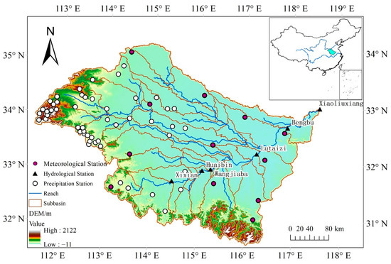
Figure 1.
Basic information of the upper Huai River basin including location, elevation, reaches, location of the meteorological, precipitation, and hydrological stations, and the subbasin delineation in SWAT modeling.
3.2. Data Preparation for SWAT Model Building
The SWAT model building requires meteorological forcing and underlying land surface data. The meteorological forcing data include precipitation, maximum and minimum air temperature, solar radiation, wind speed, and relative humidity. The precipitation data were collected from 63 precipitation and meteorological stations within the catchment (Figure 1). The other meteorological variables were recorded from 12 meteorological stations. The land surface data include terrain, land use, and soil category. The terrain data were obtained from the digital elevation model (DEM) of the basin, download from the 90m Shuttle Radar Topography Mission (SRTM) (https://search.earthdata.nasa.gov/, accessed on 1 October 2022) (Figure 1). The land use land cover data were extracted from the1km remote sensing based Chinese national land use map (Figure 2a). The catchment is predominantly covered by agricultural land, mixed forest, and residential land. The soil category data were extracted from the 1km Harmonized World Soil Database (HWSD) database (Figure 2b). The soil texture, profile stratification, and area proportion of this basin were listed in Table 1. Based on these aforementioned meteorological and underlying surface data, the upper Huai River basin was divided into 37 subbasins and further delineated into 107 HRUs.
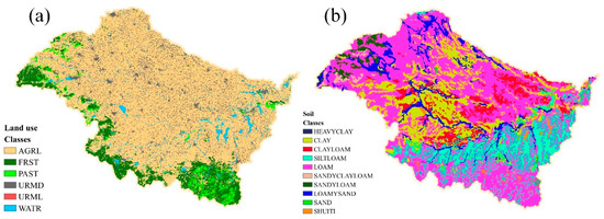
Figure 2.
(a) Land use and land cover, and (b) soil category in the upper Huai River basin. AGRL (69.9%), FRST (11.5%), PAST (3.2%), URMD (12.5%), URML (0.006%), and WATR (2.9%) represent the general agricultural land, mixed forest, pasture, residential medium density land, residential medium and low density land, and water, respectively.
3.3. Remote Sensing and In Situ SM Data
The SMAP L3 and ASCAT L2 SM data were used in this study. The SMAP SM (V8) is an estimate of the surface SM within top 5 cm of soil column based on the baseline dual channel algorithm [38]. Here, the passive L-band radiometer 36 km resolution product was used. The ASCAT SM was retrieved from the ASCAT backscatter measurements using a time-series-based change detection approach [39,40]. ASCAT is a real-aperture radar instrument measuring radar backscatter at C-band in VV polarization and scans the Earth’s surface in descending and ascending overpasses [41]. ASCAT provides SM data with a spatial resolution of 25 km and a revisit time of 1–3 days. The SMAP SM was first resampled to 25 km using the nearest neighboring method to make it consistent with the ASCAT SM. The spatial distribution of the resampled SMAP and ASCAT grids is shown in Figure 3a.
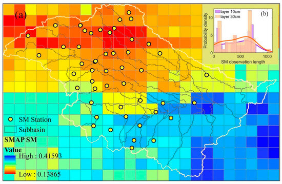
Figure 3.
(a) Location of the 51 soil moisture observation stations and the spatial distribution of the remote sensing raster data of SMAP and ASCAT, and (b) the probability distribution of the data record lengths. The colored grid pixels represent a single day of SMAP retrievals (2 February 2016).
SM observations were collected from 51 in situ stations with varying record lengths between 2016 and 2018 (hydrographic office of Henan and Shandong province in China) (Figure 3a,b). The ground-based data were used to validate the satellite SM DA efficacy on SM estimation. The validation was between the grid-based SM estimation and the in situ SM observation falling in a given grid pixel. In situ SM data were observed at the depths of 10 cm, 20 cm and 40 cm. According to the stratification scheme of soil profile, we obtained 30 cm SM values based on linear interpolation. Model simulations and satellite retrievals were validated against the in situ 10 cm SM values, considering the fact that SM in the top 5 cm and 10 cm layers have marginal differences [42,43].
4. Data Assimilation (DA) Setup
4.1. Triple Collocation (TC) Based Error Analysis
TC analysis is a method to estimate the total random error variances of three collocated measurements of the same geophysical variable [44]. It allows the intercomparison of errors obtained for three independent datasets after scaling into the same space. Currently, TC is one of the most widely used error evaluation methods for SM products in the absence of in situ SM measurements [45,46,47,48]. In this study, the three independent SM datasets are SMAP, ASCAT, and SWAT modelled SM, respectively. To ensure unbiased errors from the three independent sources, SMAP and ASCAT SM data were rescaled to the reference model estimates of SWAT by matching the cumulative distribution function (CDF) of satellite SM retrievals to that of the modelled SM [49,50]. The CDF matching was achieved by ranking datasets of satellite derived and modelled SM and fitting a five-order polynomial to the differences. Under the assumption that the three independent datasets are linearly related to the true value with additive random error in TC, the error variance (σ2) of each dataset can be estimated from the temporal variance and covariance between datasets, respectively, as follows [45]:
where x, y and z represent the rescaled SMAP, ASCAT and SWAT SM, respectively, and Q denotes the temporal variance and covariance between the three datasets.
4.2. EnKF Implementation in SWAT Model
DA aims to merge forecasted model states (i.e., the background) and observations considering their respective uncertainties to minimize the error variance in the updated (analyzed) model states. The EnKF requires an appropriate ensemble of model states to represent the background error. In this study, the ensemble of SM model states was generated by an integrative perturbation of model forcing inputs of precipitation, temperature, and model simulated SM. Precipitation at each station was perturbed by a multiplicative lognormal error with a mean of 1.0 and a standard deviation of 0.3 combing the error setting in previous research (e.g., [25,51]) and the robustness of EnKF in error processing. The maximum and minimum air temperature were perturbed by an additive normally distributed error with a standard deviation of 1.0 °C [18,21]. The modelled SM states were perturbed by an additive normally distributed error with a standard deviation of 0.02 m3/m3 for the surface layer (0–10 cm) and rootzone (10–30 cm), and a standard deviation of 0.01 m3/m3 for the deep layer (30–100 cm).
In this study, the SM DA was based on the calibrated SWAT model considering exclusively the state update. The implementation of the calibrated SWAT model with error perturbations on precipitation, temperature, and simulated SM was regarded as reference (Openloop). Preprocessing was implemented with satellite SM retrievals before DA. Systematic biases between satellite and modeled SM were corrected using the CDF rescaling method after the spatial mapping of the grid pixels and subbasins. The rescaled satellite SM was assimilated into SWAT modeling at each time step with available EnKF-based SM state updates and TC-based error characterization. Figure 4 provides the schematic overview of the Openloop, DA preprocessing, and EnKF scenario.
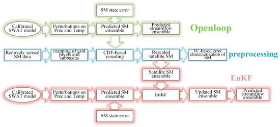
Figure 4.
Schematic overview of the model Openloop, EnKF simulation, and the DA preprocessing scheme.
The DA period was 2016–2018 after the model calibration of 2010–2015. The model calibration is based on the streamflow observations of all six hydrological stations available at the mainstream, i.e., Xixian, Huaibin, Wangjiaba, Lutaizi, Bengbu and Xiaoliuxiang (Figure 1). The distributed parameter optimization follows the principle from upstream to downstream controlling stations. The calibration processes combine the auto-calibration of the Sequential Uncertainty Fitting [52] and the manual fine-tuning method. The sensitive parameters that need to be adjusted are listed in Table 2.

Table 2.
SWAT model parameters in calibration.
4.3. Evaluation Metrics
The DA performance was evaluated by comparing the EnKF and Openloop results against the in situ SM and streamflow measurements. The bias (Bias), percent bias (PBias), Pearson’s correlation coefficient (r2), root mean square error (RMSE), unbiased RMSE (ubRMSE), and Nash–Sutcliffe coefficient of efficiency (NSE) were used as metrics. Meanwhile, the effectiveness criterion (EFF) [53] and the normalized error reduction index (NER) were used to directly assess the streamflow improvement in the EnKF over the Openloop. EFF and NER can be obtained as follows:
where n is the total time step of DA; , , and are the model predicted streamflow in the EnKF and the Openloop scenario; and the observed discharge at time t, RMSEEnKF and RMSEol are the RMSE of the modelled streamflow in the EnKF and Openloop scenario, respectively.
5. Results
5.1. Catchment Applicability of SWAT Model
Figure 5 compares the SWAT model simulated against the observed daily streamflow at the catchment outlet (Xiaoliuxiang station) in model calibration and validation phases. The hydrographs of both streamflow data generally match well during the calibration and validation phases. The evaluation statistics at the catchment outlet show good consistency of the modeling and observational results: the PBias values within ±10%, r2 > 0.8, NSE > 0.65, and RMSE < 600 m3/s (station Xiaoliuxiang in Table 3). The evaluation statistics at the other five interior hydrological stations (Table 3) indicate the relatively good performance of the SWAT model in the distributed rainfall-runoff simulation of the upper Huai River basin. For both calibration and validation phases, almost all stations have PBias values within ± 15%, r2 > 0.8, and NSE > 0.6 except for the station Xixian at the most upstream. The comparatively high consistent hydrograph and the good statistics reflect the good applicability of the SWAT model in the study catchment.
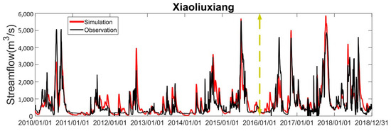
Figure 5.
The observed (Observation) and simulated (Simulation) daily streamflow at catchment outlet of the upper Huai River basin in the model calibration (2010–2016) and validation (2016–2018) phases.

Table 3.
Statistics for the model simulated streamflow at the six hydrological stations in the model calibration and validation phases.
5.2. Modeling and Observation Errors
Figure 6 presents the rescaled SMAP, ASCAT and SWAT-modeled SM errors at each grid pixel and the error probability distribution of all grid pixels within the catchment based on the TC method (Figure 3). The error standard deviation of SMAP SM and ASCAT SM vary between 0.01 and 0.03 m3/m3, and the error standard deviation of SWAT-modelled SM is less than 0.02 m3/m3. The random error of remote sensing SM is substantially larger than that of the modelled SM. Large error differences are present in the grid pixels in space with varying topography, land cover and soil (Figure 2), in particular for the ASCAT SM and SWAT modelled SM. Meanwhile, large error differences are present in the three SM datasets for a given grid pixel, demonstrating the potential benefit of SM data fusion and assimilation. The very small values of the SWAT-SM error at a few grids are likely caused by the unchanged modelling SM, for example the water body.

Figure 6.
Standard deviation of the error (Std of error) for the rescaled remote sensing (SMAP and ASCAT) and SWAT modelled soil moisture based on the TC method (i.e., the σx, σy and σz) at each grid pixel (a) and the error probability density (b).
5.3. Data Assimilation Effects on Soil Moisture
Figure 7 compares the data accuracy of the simulated SM in EnKF and Openloop scenarios based on the 51 in situ SM stations available to illustrate the SMAP SM DA effects on profile SM modeling. For the surface layer (0–10 cm), most stations have bias values within −0.1 and 0.1 m3/m3, r values within 0.2–0.6, RMSE values within −0.05–0.15 m3/m3, and ubRMSE values within 0.04–0.06 m3/m3 for the Openloop, EnKF and rescaled SMAP SM (Figure 7a–d). The corresponding statistics of the rootzone (0–30 cm) SM are comparable to those of the surface layer (Figure 7e–h). SMAP SM DA marginally reduces the biases of SM modeling (Figure 7a), yet significantly increases the correlations between the model simulated and in situ SM (Figure 7b). Meanwhile, the RMSE and ubRMSE values are largely reduced through SMAP SM assimilation (Figure 7c,d). Similar to the surface layer, the improvement in the rootzone is mainly manifested in the improved r, RMSE, and ubRMSE values (Figure 7f–h). Generally, SMAP SM is superior to SWAT simulated SM in Openloop at ~47% stations (Table 4). SMAP SM has a relatively larger (0.7%) bias, but a higher (7%) r, and a slightly lower (−0.8%) RMSE and (−2%) ubRMSE than Openloop. Integrating SMAP SM largely improves SWAT simulated SM for surface and rootzone layers at over 70% of stations. The overall improvements are −10.5%/−9.5% for Bias, 11.7%/8.8% for r, −9.5%/−10.1% for RMSE, and −7.9%/−10.9% for ubRMSE in the surface/rootzone.
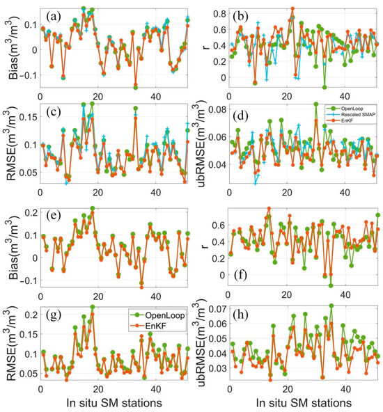
Figure 7.
Bias (a,e), r (b,f), RMSE (c,g), ubRMSE (d,h) of the rescaled SMAP SM and the estimated soil moisture in Openloop and EnKF based on the SMAP SM assimilation for the surface (0–10 cm) and rootzone (10–30 cm).

Table 4.
Comparison of bias, r, RMSE and ubRMSE for total 51 SM stations based on SMAP and ASCAT DA.
Figure 8 shows the bias, r, RMSE, and ubRMSE values for the EnKF and Openloop SM based on ASCAT SM assimilation. ASCAT SM is inferior to SWAT simulated SM in Openloop at most stations, particularly for r, RMSE and ubRMSE (Figure 8a–d). Only ~28% stations show better ASCAT SM than Openloop SM (Table 3). It seems that the ASCAT SM DA effects on SM modeling are not robust for all stations. The ASCAT SM retrievals with high data quality tend to improve SM simulation (Figure 8a–h). Statistically, the ASCAT SM assimilation improved the surface and rootzone SM at over 50% of stations, in particular for the RMSE and ubRMSE values (Table 3). The RMSE and ubRMSE are improved by −4.9%/−9.3% and −2.9%/−5.3% in the surface/rootzone.
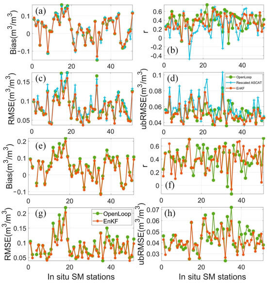
Figure 8.
Bias (a,e), r (b,f), RMSE (c,g), ubRMSE (d,h) of the rescaled ASCAT SM and the estimated soil moisture in Openloop and EnKF based on the ASCAT SM assimilation for the surface (0–10 cm) and rootzone (10–30 cm).
Overall, SMAP SM DA largely improved the surface (0–10 cm) and rootzone (10 –30cm) SM estimation in the upper Huai River basin. The effects of ASCAT SM assimilation are moderate, caused by its poor data quality in this basin.
5.4. Data Assimilation Impacts on Streamflow
Table 5 shows the effectiveness criterion (EFF) and the normalized error reduction index (NER) values of the simulated streamflow based on SMAP and ASCAT SM assimilation at five interior hydrological stations (Xixian, Huaibin, Wangjiaba, Lutaizi, and Bengbu) and the station at the catchment outlet (Xiaoliuxiang). SMAP and ASCAT SM assimilation improves the modelled streamflow at two upstream interior stations, i.e., the Huaibin and Wangjiaba satations. However, the DA does not improve the modelled streamflow at the other four stations, in particular for the downstream station (Bengbu) and the catchment outlet. It means that both SMAP SM and ASCAT SM assimilation produce un-robust impacts on the distributed streamflow modeling in the Huai River basin.

Table 5.
Statistics of the SMAP and ASCAT soil moisture assimilation impacts on streamflow simulation at the six hydrological stations in upper Huai River basin.
Figure 9 compares the SMAP SM assimilation-based and the Openloop streamflow at the Wangjiaba and Xiaoliuxiang stations. The DA has a marginal impact on streamflow modeling in the study catchment. The EnKF streamflow does not show much difference from the Openloop streamflow (the red and blue lines in Figure 9a,b). The marginal effects in streamflow can be partly impacted by the semihumid and humid climate conditions of the catchment. SM content is relatively high throughout the year, with catchment averages in most days exceeding 0.3 m3/m3, in particular for the rootzone and deep layers (Figure 10). Thereby, it leaves a limited room for improvement of streamflow simulation by enhancing SM status. Moreover, both positive and negative effects are present (see the light green and pink bands in Figure 10), suggesting the un-robust DA performance, in particular for the basin outlet. The un-robust effects might be related to the sub-optimal model parameters and the unsatisfied model structure, which cannot effectively account for the disturbances of the complex and dense human activities on the rainfall-runoff processes of the basin, for example the reservoir influences (see the gray rectangle in Figure 10b).
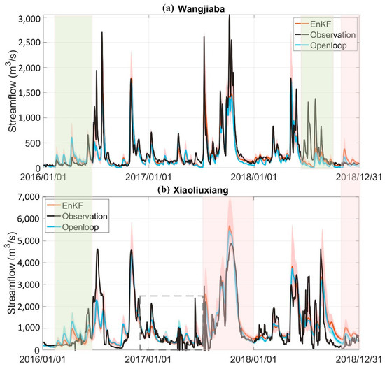
Figure 9.
The daily streamflow at the station of (a) Wangjiaba and (b) Xiaoliuxiangs in EnKF and Openloop scenarios of SMAP SM data assimilation over 2016–2018.
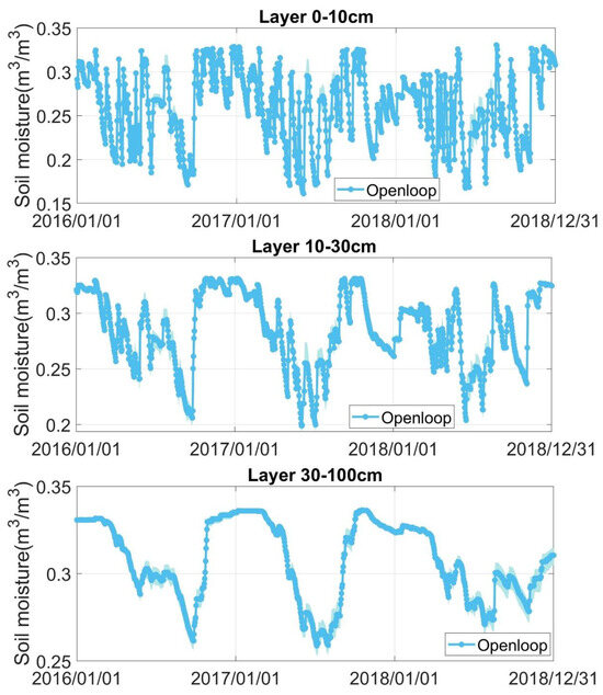
Figure 10.
The three-layer soil moisture of the basin between 2016 and 2018.
6. Discussion
We demonstrated the benefits of high-quality satellite SM to improve SWAT modeling of SM at both the surface layer and rootzone. The improved SM estimation confirmed the significance of integrating remotely sensed SM in distributed hydrological modeling of SWAT. Nevertheless, the improvements in profile SM estimation are not robust, particularly for those based on the low-quality ASCAT SM data. Analyzed SM accuracy is deteriorated at several stations, even when SMAP SM is assimilated (Figure 7 and Figure 8, Table 3). Different model error parameterizations still cannot largely improve the DA effects on SM estimation. We found error parameterizations had no significant impact on SM estimation as differences in ubRMSE values are marginal (see vertical legend in Figure 11a,b). It seems that low ubRMSE values can be obtained in the cases of high SM states and large precipitation errors. However, larger SM perturbations at each time step likely cause biases to streamflow modeling due to the truncation errors of the updated SM by the saturation water capacity, particularly for deep soil layers. Thus, the error standard deviation was set as 0.02 m3/m3 and 0.01 m3/m3, respectively, for surface/rootzone and deep-layer SM.
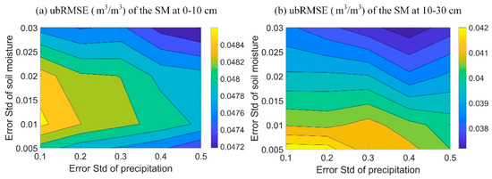
Figure 11.
The ubRMSE of the SMAP data assimilation-based SM at the (a) surface (0–10 cm) and (b) rootzone (10–30 cm).
The limited success of actual surface SM assimilation on profile soil water estimation in SWAT has also been found in previous studies (e.g., [21,51]), largely attributed to the inadequate vertical soil water coupling strength of SWAT. The correlation between surface and rootzone SM is subjected to underestimation and overestimation, varying with sites (Figure 12), despite the consideration of evaporation and evapotranspiration compensation factors in SWAT to account for varying vertical coupling in real cases. Decoupling (underestimation) limits the EnKF’s ability to update SM states of deeper layers, while over-coupling (overestimation) leads to overcorrection of deeper SM states [54]. Attempts to improve the SWAT inherent vertical coupling of soil layers were made using the ensemble of soil storages and the coupled soil moisture analytical relationship based on the EnKF [55,56]. These attempts marginally benefit the covariance-based state updates in EnKF. However, it should be acknowledged that SWAT still lacks a physical mechanism in its soil water dynamic module, so integrating a physically based module, for example the Richards equation, should be a candidate solution to this issue.
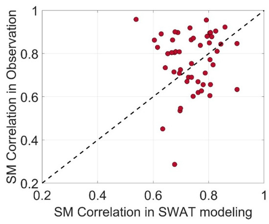
Figure 12.
Relationship of the soil moisture correlation in SWAT modeling and in situ observation between the surface layer and rootzone.
In addition to the vertical coupling issue of the model, suboptimal model calibration is also responsible for the un-robust improvements in SM, particularly for streamflow. It is a challenging task to seek optimal parameters for distributed hydrological models, due to the large number of parameters and the well-known parameter equifinality issue [57,58]. In the current study, we can hardly fine-tune the best-for-all parameters for the rainfall-runoff module based on data from six discharge stations. Extreme streamflow (low and high) is inclined to be more biased with suboptimal parameters [59]. Thus, the pre-parameter calibration is highly needed to improve streamflow modeling in the state-update DA scheme. The combined state-parameter update likely provides a viable solution (e.g., [8,60,61]).
Human manipulation of river discharges partly explains the poor DA performance on streamflow simulation. We obtained improved streamflow in the upstream regions with less intensive human activities, whereas neutral impacts or even deterioration of accuracy were found in the densely populated downstream regions (Figure 1, Table 3). Human alterations of hydrological processes increase the uncertain effectiveness of DA. It requires a more sophisticated model structure to account for these human activities. The humid and subhumid climate of the catchment are also responsible for the marginal DA effects on streamflow. The relatively high SM throughout the year tends to leave limited room for streamflow improvement by enhancing SM status. Additionally, data quality of satellite SM is another hinderance to improve streamflow simulations based on DA. Future enhancement on satellite SM observation and retrieval is essential for its effective application in hydrological modeling and prediction. Assimilating multisource data is also a promising approach to couple big data with hydrological models by separately accounting for multiple sources of uncertainty under the DA framework [62,63,64].
7. Conclusions
The DA impacts of satellite SM on distributed hydrological modeling of SWAT are investigated based on the EnKF considering the observation error using the TC method. The investigation focused on the DA effects on the surface and rootzone SM, as well as the streamflow estimation of a highly human disturbed catchment in China, i.e., the upper Huai River basin with dense in situ SM and streamflow observations. Our results show the following:
- (1)
- SWAT has good applicability in the daily rainfall-runoff simulation of the upper Huai River basin. The PBias values are generally within ±15%, r2 > 0.8, and NSE > 0.60 at the validation stations.
- (2)
- The random error standard deviation of SMAP and ASCAT SM varies between 0.01 m3/m3 and 0.03 m3/m3 for all grid pixels within the basin. Large error differences are present in the SM datasets and in different grid pixels.
- (3)
- SMAP SM DA largely improves the surface and rootzone SM estimation. Nevertheless, ASCAT SM DA gains mixed impacts on performance in SM estimation, primarily due to poor data quality.
- (4)
- The satellite SM DA does not improve streamflow simulation as effectively as SM itself. The effects of SMAP and ASCAT SM assimilation on distributed streamflow simulation are un-significant and not robust.
Overall, this study presents strong evidence of integrating satellite SM in hydrological modeling in improving SM estimation and provides implications for achieving the added value of remotely sensed SM in streamflow improvement. Satellite SM retrievals do have great capacity to improve the distributed hydrological simulation of SWAT, in particular for SM estimation. However, current benefits from DA effects are still limited by the vertical soil water coupling of SWAT, suboptimal model parameters, satellite SM data quality, humid climate, and the human disturbances on catchment rainfall-runoff process. In future, more efforts should be paid to the improvement in model structure, satellite SM retrieval, and multi-source data assimilation.
Author Contributions
Y.L. (Yongwei Liu): Conceptualization, data curation, formal analysis, investigation, methodology, validation, visualization, writing—original draft, writing—review & editing. W.C. and X.F.: methodology, writing—review & editing. J.D., Y.L. (Yuanbo Liu) and W.W.: methodology, conceptualization and supervision. Z.L., C.L. and R.W.: Data collection and processing. All authors have read and agreed to the published version of the manuscript.
Funding
This work was supported by the National Key R&D Program of China (2018YFE0105900), the National Natural Science Foundation of China (42271040, 41901049, 41961134003), the Key Deployment Projects of Sino-Africa Joint Research Center, Chinese Academy of Sciences (SAJC202106), and the International Collaboration Program of Chinese Academy of Science (151542KYSB20200015).
Data Availability Statement
The data that support the findings is available upon reasonable request.
Conflicts of Interest
The authors declare no conflict of interest.
References
- Wanders, N.; Bierkens, M.F.P.; Jong, S.M.; Roo, A.; Karssenberg, D. The benefits of using remotely sensed soil moisture in parameter identification of large-scale hydrological models. Water Resour. Res. 2014, 50, 6874–6891. [Google Scholar] [CrossRef]
- Seneviratne, S.I.; Corti, T.; Davin, E.L.; Hirschi, M.; Jaeger, E.B.; Lehner, I.; Orlowsky, B.; Teuling, A.J. Investigating soil moisture–climate interactions in a changing climate: A review. Earth Sci. Rev. 2010, 99, 125–161. [Google Scholar] [CrossRef]
- Liu, Y.W.; Liu, Y.B.; Wang, W.; Zhou, H.; Tian, L. Historical droughts manifest an abrupt shift to a wetter Tibetan Plateau. Hydrol. Earth Syst. Sci. 2022, 26, 3825–3845. [Google Scholar] [CrossRef]
- Brocca, L.; Melone, F.; Moramarco, T. On the estimation of antecedent wetness conditions in rainfall–runoff modelling. Hydrol. Process. 2008, 22, 629–642. [Google Scholar] [CrossRef]
- Massari, C.; Camici, S.; Ciabatta, L.; Brocca, L. Exploiting satellite-based surface soil moisture for flood forecasting in the Mediterranean area: State update versus rainfall correction. Remote Sens. 2018, 10, 292. [Google Scholar] [CrossRef]
- Crow, W.; Bindlish, R.; Jackson, T.J. The added value of spaceborn passive microwave soil moisture retrievals for forecasting rainfall-runoff partitioning. Geophys. Res. Lett. 2005, 32. [Google Scholar] [CrossRef]
- Leroux, D.J.; Pellarin, T.; Vischel, T.; Cohard, J.-M.; Gascon, T.; Gibon, F.; Mialon, A.; Galle, S.; Peugeot, C.; Seguis, L. Assimilation of SMOS soil moisture into a distributed hydrological model and impacts on the water cycle variables over the Ouémé catchment in Benin. Hydrol. Earth Syst. Sci. 2016, 20, 2827–2840. [Google Scholar] [CrossRef]
- Liu, Y.W.; Wang, W.; Hu, Y. Investigating the impact of surface soil moisture assimilation on state and parameter estimation in SWAT model based on the ensemble Kalman filter in upper Huai River basin. J. Hydrol. Hydromech. 2017, 65, 123–133. [Google Scholar] [CrossRef]
- Yang, H.; Xiong, L.; Liu, D.; Cheng, L.; Chen, J. High spatial resolution simulation of profile soil moisture by assimilating multi-source remote-sensed information into a distributed hydrological model. J. Hydrol. 2021, 597, 126311. [Google Scholar] [CrossRef]
- Wang, D.; Chen, Y.; Cai, X. State and parameter estimation of hydrologic models using the constrained ensemble Kalman filter. Water Resour. Res. 2009, 45, w11416. [Google Scholar] [CrossRef]
- Aubert, D.; Loumagne, C.; Oudin, L. Sequential assimilation of soil moisture and streamflow data in a conceptual rainfall–runoff model. J. Hydrol. 2003, 280, 145–161. [Google Scholar] [CrossRef]
- Fu, X.; Zhang, Y.; Zhong, Q.; Lü, H.; Ding, Y.; Li, Z.; Yu, Z.; Jiang, X. Soil moisture estimation by assimilating in-situ and SMAP surface soil moisture using unscented weighted ensemble Kalman filter. Water Resour. Res. 2023, 59, e2023WR034506. [Google Scholar] [CrossRef]
- Yu, Z.; Fu, X.; Luo, L.; Lü, H.; Ju, Q.; Liu, D.; Kalin, A.D.; Huang, D.; Yang, C.; Zhao, L. One-dimensional soil temperature simulation with Common Land Model by assimilating in situ observations and MODIS LST with the temperature simulation with Common Land Model by assimilating in situ observations and MODIS LST with the ensemble particle filter. Water Resour. Res. 2014, 50, 6950–6965. [Google Scholar] [CrossRef]
- Sahoo, A.K.; Lannoy, G.J.M.D.; Reichle, R.H.; Houser, P.R. Assimilation and downscaling of satellite observed soil moisture over the Little River Experimental Watershed in Georgia, USA. Adv. Water Resour. 2013, 52, 19–33. Available online: https://linkinghub.elsevier.com/retrieve/pii/S0309170812002357 (accessed on 9 January 2024). [CrossRef]
- Ines, A.V.M.; Das, N.N.; Hansen, J.W.; Njoku, E.G. Assimilation of remotely sensed soil moisture and vegetation with a crop simulation model for maize yield prediction. Remote Sens. Environ. 2013, 138, 149–164. [Google Scholar] [CrossRef]
- Alvarez-Garreton, C.; Ryu, D.; Western, A.W.; Su, C.H.; Crow, W.T.; Robertson, D.E.; Leahy, C. Improving operational flood ensemble prediction by the assimilation of satellite soil moisture: Comparison between lumped and semi-distributed schemes. Hydrol. Earth Syst. Sci. 2015, 19, 1659–1676. [Google Scholar] [CrossRef]
- Lievens, H.; Tomer, S.K.; Al Bitar, A.; De Lannoy, G.J.M.; Drusch, M.; Dumedah, G.; Hendricks Franssen, H.J.; Kerr, Y.H.; Martens, B.; Pan, M.; et al. SMOS soil moisture assimilation for improved hydrologic simulation in the Murray Darling Basin. Australia. Remote Sens. Environ. 2015, 168, 146–162. [Google Scholar] [CrossRef]
- Liu, Y.W.; Wang, W.; Liu, Y. ESA CCI Soil Moisture Assimilation in SWAT for Improved Hydrological Simulation in Upper Huai River Basin. Adv. Meteorol. 2018, 2018, 7301314. [Google Scholar] [CrossRef]
- Khaki, M.; Hendricks Franssen, H.J.; Han, S.C. Multi-mission satellite remote sensing data for improving land hydrological models via data assimilation. Sci. Rep. 2020, 10, 18791. [Google Scholar] [CrossRef]
- Santis De, D.; Biondi, D.; Crow, W.T.; Camici, S.; Modanesi, S.; Brocca, L.; Massari, C. Assimilation of satellite soil moisture products for river flow prediction: An extensive experiment in over 700 catchments throughout Europe. Water Resour. Res. 2021, 57, e2021WR029643. [Google Scholar] [CrossRef]
- Chen, F.; Crow, W.T.; Starks, P.J.; Moriasi, D.N. Improving hydrologic predictions of a catchment model via assimilation of surface soil moisture. Adv. Water Resour. 2011, 34, 526–536. [Google Scholar] [CrossRef]
- Crow, W.T.; Ryu, D. A new data assimilation approach for improving runoff prediction using remotely-sensed soil moisture retrievals. Hydrol. Earth Sys. Sci. 2009, 13, 1–16. [Google Scholar] [CrossRef]
- Han, E.; Merwade, V.; Heathman, G.C. Implementation of surface soil moisture data assimilation with watershed scale distributed hydrological model. J. Hydrol. 2012, 416–417, 98–117. [Google Scholar] [CrossRef]
- Reichle, R.H.; Crow, W.T.; Keppenne, C.L. An adaptive ensemble Kalman filter for soil moisture data assimilation. Water Resour. Res. 2008, 44, 423. [Google Scholar] [CrossRef]
- Xie, X.; Zhang, D. Data assimilation for distributed hydrological catchment modeling via ensemble Kalman filter. Adv. Water Resour. 2010, 33, 678–690. [Google Scholar] [CrossRef]
- Lei, F.; Huang, C.; Shen, H.; Li, X. Improving the estimation of hydrological states in the SWAT model via the ensemble Kalman smoother: Synthetic experiments for the Heihe River Basin in northwest China. Adv. Water Resour. 2014, 67, 32–45. [Google Scholar] [CrossRef]
- Brocca, L.; Moramarco, T.; Dorigo, W.; Wagner, W. Assimilation of satellite soil moisture data into rainfall-runoff modelling for several catchments worldwide. In Proceedings of the 2013 IEEE International Geoscience and Remote Sensing Symposium-IGARSS, Melbourne, VIC, Australia, 21–26 July 2013; pp. 2281–2284. [Google Scholar] [CrossRef]
- Corato, G.; Matgen, P.; Fenicia, F.; Schlaffer, S.; Chini, M. Assimilating satellite derived soil moisture products into a distributed hydrological model. In Proceedings of the 2014 IEEE Geoscience and Remote Sensing Symposium, Quebec City, QC, Canada, 13–18 July 2014; pp. 3315–3318. [Google Scholar] [CrossRef]
- Nayak, A.K.; Biswal, B.; Sudheer, K.P. Role of hydrological model structure in the assimilation of soil moisture for streamflow prediction. J. Hydrol. 2021, 598, 126465. [Google Scholar] [CrossRef]
- Massari, C.; Brocca, L.; Tarpanelli, A.; Moramarco, T. Data assimilation of satellite soil moisture into rainfall-runoff modelling: A complex recipe? Remote Sens. 2015, 7, 11403–11433. [Google Scholar] [CrossRef]
- Fu, X.; Jiang, X.; Yu, Z.; Ding, Y.; Lü, H.; Zheng, D. Understanding the key factors that influence soil moisture estimation using the unscented weighted ensemble Kalman filter. Agric. For. Meteorol. 2022, 313, 108745. [Google Scholar] [CrossRef]
- Brocca, L.; Moramarco, T.; Melone, F.; Wagner, W.; Hasenauer, S.; Hahn, S. Assimilation of Surface-and Root-Zone ASCAT Soil Moisture Products Into Rainfall–Runoff Modeling. IEEE Trans. Geosci. Remote Sens. 2015, 50, 2542–2555. [Google Scholar] [CrossRef]
- Dorigo, W.A.; Gruber, A.; De Jeu, R.A.M.; Wagner, W.; Stacke, T.; Loew, A.; Kidd, R. Evaluation of the ESA CCI soil moisture product using ground-based observations. Remote Sens. Environ. 2015, 162, 380–395. [Google Scholar] [CrossRef]
- Neitsch, S.L.; Arnold, J.G.; Kiniry, J.R.; Williams, J.R. Soil and Water Assessment Tool Theoretical Documentation Version 2009; TR-406, Texas Water Resources Institute Technical Report No.406; Texax A&M University: College Station, TX, USA, 2011; Available online: http://swat.tamu.edu/media/99192/swat2009theory.pdf (accessed on 9 January 2024).
- Monteith, J.L. Evaporation and the environment. In 19th Symposia of the Society for Experimental Biology: The State and Movement of Water in Living Organisms; Cambridge University Press: London, UK, 1965; pp. 205–234. [Google Scholar]
- Evensen, G. Sequential data assimilation with a nonlinear quasi-geostrophic model using Monte Carlo methods to forecast error statistics. Journal of Geophysical methods to forecast error statistics. J. Geophys. Res.-Ocean 1994, 99, 10143–10162. [Google Scholar] [CrossRef]
- Evensen, G. The Ensemble Kalman Filter: Theoretical formulation and practical implementation. Ocean Dynam. 2003, 53, 343–367. [Google Scholar] [CrossRef]
- O’Neill, P.E.; Chan, S.; Njoku, E.G.; Jackson, T.; Bindlish, R.; Chaubell, J. L3 Radiometer Global Daily 36 km EASE-Grid Soil Moisture, Version 8; NASA National Snow and Ice Data Center Distributed Active Archive Center: Boulder, CO, USA, 2021. [Google Scholar] [CrossRef]
- Wagner, W.; Lemoine, G.; Rott, H. A method for estimating soil moisture from ERS scatterometer and soil data. Remote Sens. Environ. 1999, 70, 191–207. [Google Scholar] [CrossRef]
- Naeimi, V.; Scipal, K.; Bartalis, Z.; Hasenauer, S.; Wagner, W. An improved soil moisture retrieval algorithm for ERS and METOP scatterometer observations. IEEE Trans. Geosci. Remote Sens. 2009, 47, 1999–2013. [Google Scholar] [CrossRef]
- Zeng, J.; Li, Z.; Chen, Q.; Bi, H.; Qiu, J.; Zou, P. Evaluation of remotely sensed and reanalysis soil moisture products over the Tibetan Plateau using in-situ observations. Remote Sens. Environ. 2015, 163, 91–110. [Google Scholar] [CrossRef]
- Shellito, P.J.; Small, E.E.; Livneh, B. Controls on surface soil drying rates observed by smap and simulated by the noah land surface model. Hydrol. Earth Syst. Sci. 2018, 22, 1649–1663. [Google Scholar] [CrossRef]
- Dong, J.Z.; Crow, W.T.; Tobin, K.J.; Cosh, M.H.; Bosch, D.D.; Starks, P.J.; Seyfried, M.; Collins, C.H. Comparison of microwave remote sensing and land surface modeling for surface soil moisture climatology estimation. Remote Sens. Environ. 2020, 242, 111756. [Google Scholar] [CrossRef]
- Stoffelen, A. Toward the true near-surface wind speed: Error modeling and calibration using triple collocation. J. Geophys. Res. 1998, 103, 7755–7766. [Google Scholar] [CrossRef]
- McColl, K.A.; Vogelzang, J.; Konings, A.G.; Entekhabi, D.; Piles, M.; Stoffelen, A. Extended triple collocation: Estimating errors and correlation coefficients with respect to an unknown target. Geophys. Res. Lett. 2014, 41, 6229–6236. [Google Scholar] [CrossRef]
- Dorigo, W.; Wagner, W.; Albergel, C.; Albrecht, F.; Balsamo, G.; Brocca, L.; Chung, D.; Ertl, M.; Forkel, M.; Gruber, A. ESA CCI Soil Moisture for improved Earth system understanding: State-of-the art and future directions. Remote Sens. Environ. 2017, 203, 185–215. [Google Scholar] [CrossRef]
- Crow, W.; Van den Berg, M. An improved approach for estimating observation and model error parameters in soil moisture data assimilation. Water Resour. Res. 2010, 46, W12519. [Google Scholar] [CrossRef]
- Su, C.H.; Ryu, D.; Crow, W.T.; Western, A.W. Beyond triple collocation: Applications to soil moisture monitoring. J. Geophys. Res.-Atmos. 2014, 119, 6419–6439. [Google Scholar] [CrossRef]
- Reichle, R.H.; Koster, R.D. Bias reduction in short records of satellite soil moisture. Geophys. Res. Lett. 2004, 31, L19501. [Google Scholar] [CrossRef]
- Scipal, K.; Drusch, M.; Wagner, W. Assimilation of a ERS scatterometer derived soil moisture index in the ECMWF numerical weather prediction system. Adv. Water Resour. 2008, 31, 1101–1112. [Google Scholar] [CrossRef]
- Clark, M.P.; Rupp, D.E.; Woods, R.A.; Zheng, X.; Ibbitt, R.P.; Slater, A.G.; Schmidt, J.; Uddstrom, M.J. Hydrological data assimilation with the ensemble Kalman filter: Use of streamflow observations to update states in a distributed hydrological model. Adv. Water Resour. 2008, 31, 1309–1324. [Google Scholar] [CrossRef]
- Abbaspour, K.; Johnson, C.; Van Genuchten, M.T. Estimating uncertain flow and transport parameters using a sequential uncertainty fitting procedure. Vadose Zone J. 2004, 3, 1340–1352. [Google Scholar] [CrossRef]
- Chen, H.; Yang, D.; Hong, Y.; Gourley, J.J.; Zhang, Y. Hydrological data assimilation with the ensemble square-root-filter: Use of streamflow observations to update model states for real-time flash flood forecasting. Adv. Water Resour. 2013, 59, 209–220. [Google Scholar] [CrossRef]
- Kumar, S.V.; Reichle, R.H.; Koster, R.D.; Crow, W.T.; Peters-Lidard, C.D. Role of Subsurface Physics in the Assimilation of Surface Soil Moisture Observations. J. Hydrometeor. 2009, 10, 1534–1547. [Google Scholar] [CrossRef]
- Patil, A.; Ramsankaran, R. Improving streamflow simulations and forecasting performance of SWAT model by assimilating remotely sensed soil moisture observations. J. Hydrol. 2017, 555, 683–696. [Google Scholar] [CrossRef]
- Patil, A.; Ramsankaran, R. Improved streamflow simulations by coupling soil moisture analytical relationship in EnKF based hydrological data assimilation framework. Adv. Water Resour. 2018, 121, 173–188. [Google Scholar] [CrossRef]
- Beven, K.; Freer, J. Equifinality, data assimilation, and uncertainty estimation in mechanistic modelling of complex environmental systems using the GLUE methodology. J. Hydrol. 2001, 249, 11–29. [Google Scholar] [CrossRef]
- Abbaspour, K.C.; Rouholahnejad, E.; Vaghefi, S.; Srinivasan, R.; Yang, H.; Kløve, B. A continental-scale hydrology and water quality model for Europe: Calibration and uncertainty of a high-resolution large-scale SWAT model. J. Hydrol. 2015, 524, 733–752. [Google Scholar] [CrossRef]
- Dong, J.Z.; Lei, F.N.; Crow, W. Land transpiration-evaporation partitioning errors responsible for modeled summertime warm bias in the central United States. Nat. Commun. 2022, 13, 336. [Google Scholar] [CrossRef] [PubMed]
- Xie, X.; Zhang, D. A partitioned update scheme for state-parameter estimation of distributed hydrologic models based on the ensemble Kalman filter. Water Resour. Res. 2013, 49, 7350–7365. [Google Scholar] [CrossRef]
- Sun, L.; Seidou, O.; Nistor, I. Data assimilation for streamflow forecasting: State-parameter assimilation versus output assimilation. J. Hydrol. Eng. 2017, 22, 04016060. [Google Scholar] [CrossRef]
- Sun, L.; Seidou, O.; Nistor, I.; Goïta, K.; Magagi, R. Simultaneous assimilation of in situ soil moisture and streamflow in the SWAT model using the Extended Kalman Filter. J. Hydrol. 2016, 543, 671–685. [Google Scholar] [CrossRef]
- Avellaneda, P.M.; Ficklin, D.L.; Lowry, C.S.; Knouft, J.H.; Hall, D.M. Improving hydrological models with the assimilation of crowdsourced data. Water Resour. Res. 2020, 56, e2019WR026325. [Google Scholar] [CrossRef]
- Azimi, S.; Dariane, A.B.; Modanesi, S.; Bauer-Marschallinger, B.; Bindlish, R.; Wagner, W.; Massari, C. Assimilation of Sentinel 1 and SMAP–based satellite soil moisture retrievals into SWAT hydrological model: The impact of satellite revisit time and product spatial resolution on flood simulations in small basins. J. Hydrol. 2020, 581, 124367. [Google Scholar] [CrossRef]
Disclaimer/Publisher’s Note: The statements, opinions and data contained in all publications are solely those of the individual author(s) and contributor(s) and not of MDPI and/or the editor(s). MDPI and/or the editor(s) disclaim responsibility for any injury to people or property resulting from any ideas, methods, instructions or products referred to in the content. |
© 2024 by the authors. Licensee MDPI, Basel, Switzerland. This article is an open access article distributed under the terms and conditions of the Creative Commons Attribution (CC BY) license (https://creativecommons.org/licenses/by/4.0/).