Combining Satellite Optical and Radar Image Data for Streamflow Estimation Using a Machine Learning Method

Abstract

River water surface extent can be extracted from optical and radar satellite images; this is useful for estimating streamflow from space. The radiation characteristics of open water from the visible and microwave bands are different and provide independent information. In this study, for the purpose of improving streamflow estimation from space for data-sparse regions, a method that combines satellite optical and radar images data for streamflow estimation using a machine learning technique was proposed. The method was demonstratedthrough a case study in the river segment upstream of the Ganzi gauging station on the Yalong River, China. Utilizing the support vector regression (SVR) model, the feasibility of different combinations of water surface area derived from Sentinel-1 synthetic aperture radar images (AREA_SAR), modified normalized difference water index derived from Landsat 8 images (MNDWI), and reflectance ratios between NIR and SWIR channels derived from MODIS images (R_NIR/R_SWIR) for streamflow estimation were evaluated through three experiments. In Experiment I, three models using AREA_SAR (Model 1), MNDWI (Model 2), and a combination of AREA_SAR and MNDWI (Model 3) were built; the mean relative error (MRE) and mean absolute error (MAE) of streamflow estimates corresponding to the SVR model using both AREA_SAR and MNDWI (Model 3) were 0.19 and 31.6 m³/s for the testing dataset, respectively, and were lower than two models using AREA_SAR (Model 1) or MNDWI (Model 2) solely as inputs. In Experiment II, three models with AREA_SAR (Model 4), R_NIR/R_SWIR (Model 5), and a combination of AREA_SAR and R_NIR/R_SWIR (Model 6) as inputs were developed; the MRE and MAE for the model using AREA_SAR and R_NIR/R_SWIR (Model 6) were 0.25 and 56.5 m³/s, respectively, which outperformed the two models treating AREA_SAR (Model 4) or MNDWI (Model 5) as single types of inputs. In Experiment III, three models using AREA_SAR (Model 7), MNDWI, and R_NIR/R_SWIR (Model 8) and the combination of AREA_SAR, MNDWI and R_NIR/R_SWIR (Model 9) were built; combining all three types of satellite observations (Model 9) exhibited the highest accuracy, for which the MRE and MAE were 0.18 and 18.4 m³/s, respectively. The results of all three experiments demonstrated that integrating optical and microwave observations could improve the accuracy of streamflow estimates using a data-driven model; the proposed method has great potential for near-real-time estimations of flood magnitude or to reconstruct past variations in streamflow using historical satellite images in data-sparse regions.

1. Introduction

As a key indicator of hydrological variation, river discharge contains abundant information about the water cycle at basin scale. Observations or predictions of streamflows can provide important support for water resource management and flood disaster prevention [1]. However, most areas around the globe have not yet established a complete ground-based hydrological observation system subject to factors of adverse geographic condition [2], maintenance costs [3], or political constraints [4,5], and the availability of existing hydrological observation networks is declining [6]. Hydrological and hydraulic modeling are common tools for streamflow estimation [7], but they require many types of data about the physical conditions of the region being modeled, which limits their application in ungauged basins. With the rapid development of remote sensing technology in the past few decades, several hydraulic variables related to streamflow can be extracted, i.e., water surface level, water surface elevation, and river channel slope. Many studies have established empirical relationships [8,9,10] between single or multivariate satellite observations and measured streamflows, showing great potential for estimating streamflow from space.

Among satellite-observable river hydraulics, the water surface level is the most preferable for streamflow estimation, as it possesses the strongest relationship with streamflow and is commonly used in regular ground observations for scaling streamflow [11,12]. Observations from satellite radar altimetry have been widely used for streamflow estimations [13,14,15]. However, low spatial coverage gives rise to limitations in its application to streamflow estimation; for space-borne radar altimetry technology, only one-dimensional observations of water level are available, at the point where satellite ground tracks intersect the river [16]. The distance between two adjacent satellite orbits usually ranges from 80 (ERS-2 and ENVISAT-series) to 315 km (TOPEX-series) [17]. The newly launched Surface Water and Ocean Topography (SWOT) mission [18] at the end of 2020 can provide water level and water surface extent observations simultaneously for most middle-to-large rivers globally, which could fill the gap of one-dimensional radar altimetry. However, it is difficult to trace streamflow information back over the past few decades using SWOT, when the hydrological cycle experiences significant changes due to human activity. In this context, river water surface extent or width has the value of tracing streamflow over the past five decades. Since the Landsat 1 launched into space in the early 1970s [19], many Earth-observing satellites have been collecting huge numbers of images of Earth’s surface. Either from optical or synthetic aperture radar (SAR) images, abundant radiation information is useful for extracting river water surface extent. Additionally, their feasibility for streamflow estimations have been demonstrated in many studies [20,21,22].

For traditional empirical methods, the river water surface extent or river width need to be inverted from spectral and radiative observations from remote sensing, before building statistical relationship to estimate streamflow. Many satellite observations with low spatial resolution may not provide accurate estimations of the river water surface extent. However, their frequency of observation is much higher than that of high-resolution satellite observations, and they consequently contain a huge amount of information about changes in streamflow. For example, MODIS could provide nearly daily observations with a low resolution of several hundred meters. Under the empirical method framework, such coarse satellite observations cannot estimate streamflow with satisfactory accuracy for middle-to-small rivers. Meanwhile, river water surface reflectance from synthetic aperture radar (SAR) or multispectral indices (e.g., modified normalized difference water index (MNDWI)) have strong physical correlations with streamflow, but their unclear physical relationship makes it difficult to estimate river streamflow. Machine learning techniques (MLTs) provide an opportunity to directly track relationships between spectral and radiative signals of river water surface and streamflow. Such techniques have the potential to identify the complex nonlinear input–output relationships without explicitly understanding physical mechanisms between variables. MLTs focus on discovering the intrinsic patterns of data and have been used in the study of streamflow, flood susceptibility, and sediment estimation [23,24,25,26]. Sahoo [27] integrated satellite reflectance with different machine learning algorithms (i.e., artificial neural network (ANN), random forest regression (RFR), and support vector regression (SVR)) for ecological flow regime estimations in a typical Brahmani River Basin of India. In Zaji’s study [28], the brightness temperature was used as the input for three MLT-based methods, i.e., multilayer perceptron (MP), extreme learning machines (ELMs), and radial basis function (RBF), for improving the accuracy of river discharge prediction on the Connecticut River. MLTs also provide a chance to integrate river hydraulics observed from different satellite sensors for streamflow estimations. Tarpanelli [17] merged the reflectance ratio of a dry pixel (C) to a wet pixel (M) with altimetry data to estimate river discharge using ANN techniques, at Lokoja along the Niger River and Pontelagoscuro along the Po River. In optical and SAR satellite images, information about the river water surface was detected from visible and microwave spectra, respectively. The information describes the characteristics of water surface areas from different and independent aspects. Integration of this information using MLTs may improve streamflow estimation from one single type of satellite observation.

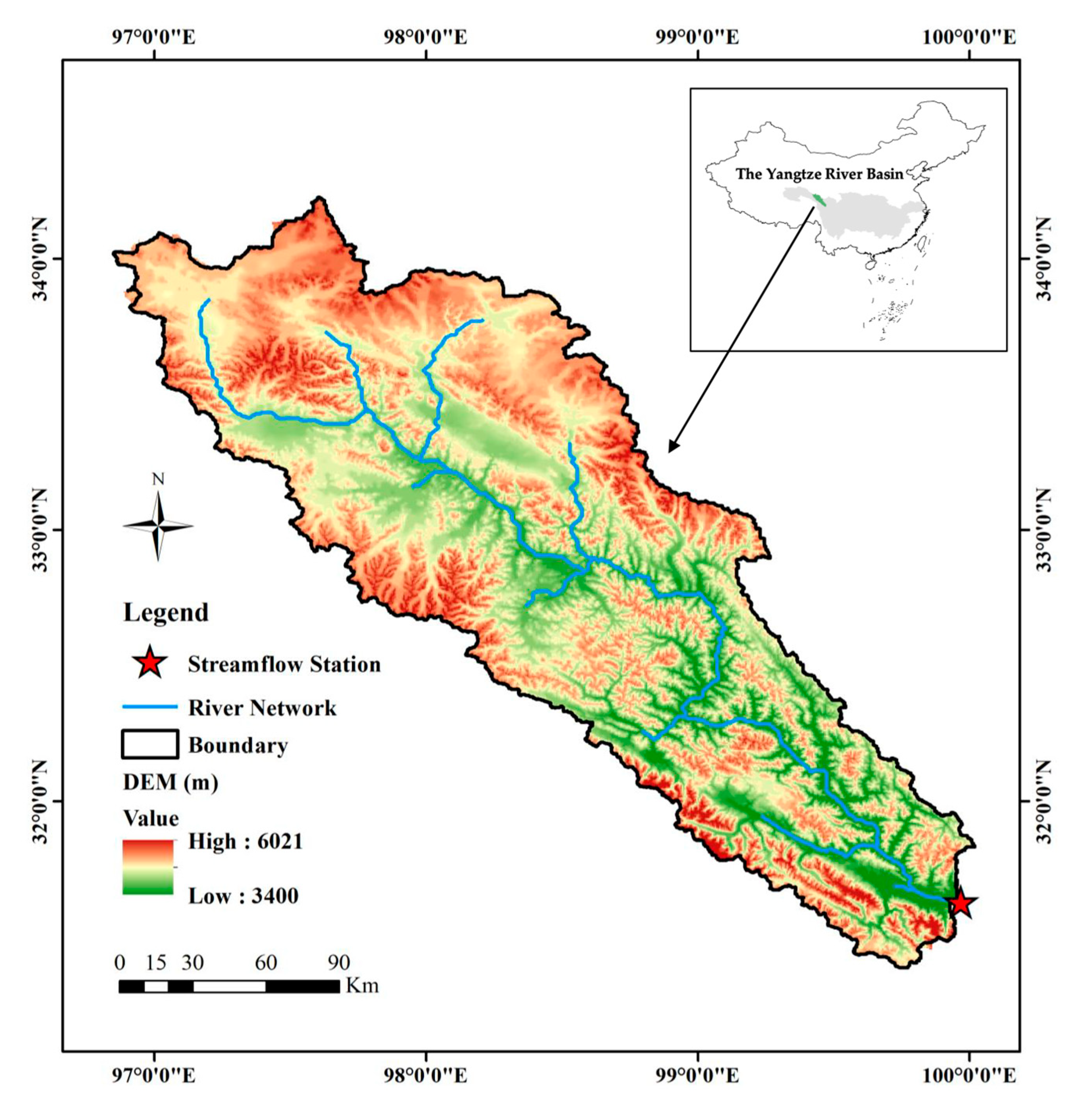
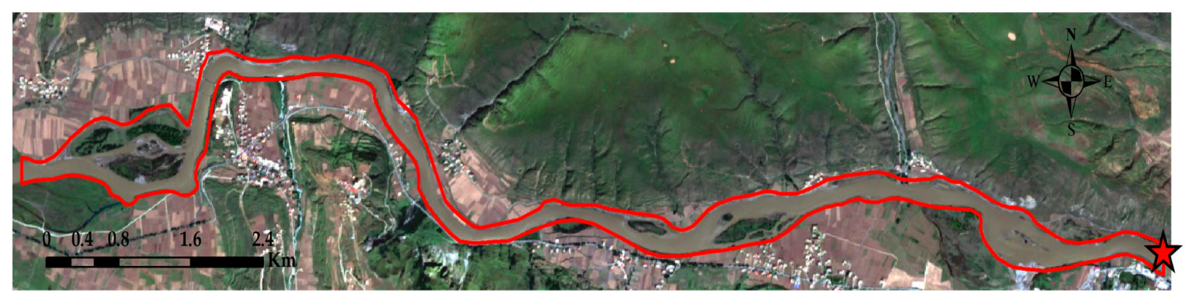
Based on this understanding, the objective of this study was to develop a method for integrating remotely sensed information about river water surfaces derived from optical images and SAR images for streamflow estimation. For the river segment upstream of Ganzi gauging station in the Yalong River, which is located in the Qinghai–Tibet Plateau and is a major tributary of the Yangtze River, variations in water surface were detected from Landsat and MODIS optical images and Sentinel-1 SAR images, and then combined for streamflow estimation using the SVR method. By comparing the results of streamflow estimation using single or multiple satellite observations, the value of integrating information from different sources was evaluated. This study’s contribution is providing a new method for reproducing streamflow variations from over the past few decades and giving some insights into how to more effectively combine information from different types of remote sensing data for streamflow estimation.

2. Study Area and Datasets

2.1. Study Area

In this study, the streamflow of the Ganzi Hydrological Station in the Yalong River, China, was estimated to test the feasibility of the proposed method. The Yalong River is one of the largest tributaries of the upper Yangtze River in China, located in the southeast Qinghai–Tibetan Plateau (Figure 1). The upstream region of the Ganzi Station has a catchment area of 33,000 km². The altitude ranges from 3400 m to 6200 m. The terrain is predominantly mountainous, with a transition from hilly plateaus to alpine gorges from north to south. The climate zone covers the semi-humid area of the plateau sub-frigid zone and the arid area of the plateau cold zone, with clear plateau characteristics. The average annual precipitation ranges from 600 to 800 mm, and due to the influence of altitude, the annual snowfall period lasts for more than 9 months; annual snowfall accounts for approximately 40–70% of the annual precipitation. The dry and wet seasons are clearly distinct in the upstream Yalong River catchment, with the wet season from May to October contributing 80% of the mean annual runoff. Due to poor geographical conditions, there are only a few, but very important, hydrological stations distributed in the Yalong River Basin, among which is the Ganzi gauging station, situated at geographical coordinates of 99°58′E and 31°37′N.

2.2. Datasets

In this study, the satellite optical images included Landsat 8 and MODIS data. The radar images used were SAR data from Sentinel-1. From these satellite images, water surface information for the river segment upstream of Ganzi station, with a length of 13.8 km (Figure 2), was extracted and subsequently used for streamflow estimation.

Landsat 8 multispectral images with a spatial resolution of 30 m and a 16-day revisit cycle were used to obtain atmospherically corrected surface reflectance data from 2013 to 2020. In order to obtain as many intact and cloud-free images as possible, we performed a cloud-removing operation, and screening was carried out using the threshold of the percentage of cloud cover being less than 40%. After the screening, only 54 images were available. For MODIS observations, the MOD09GA product was adopted to extract water surface information, which had been corrected for atmospheric gases and aerosols. It is a daily dataset with a spatial resolution of 500 m. The degree of cloud coverage was checked for all images in the period of 2010 to 2020; 752 images met the standard.

The Sentinel-1 mission, composed of two radar satellites (i.e., 1A and 1B), provides data with a spatial resolution of 10 m from a dual-polarization C-band SAR instrument at 5.405 GHz. The revisit cycle of a single satellite is 12 days and can be increased to 6 days for a dual satellite. The Ground Range Detected (GRD) product was pre-processed using the Sentinel-1 Toolbox to convert the raw data into backscatter coefficients for storage. In this study, 300 images from 2014 to 2020 were used to map the water surface. In addition to the standard pre-processing steps of border noise removal, thermal noise removal, radiometric calibration, and terrain correction [29], the Refined Lee filter [30] was employed to remove granular noise.

Considering that the river channel width at Ganzi station is around 100 m, both Landsat 8 and MODIS images are too coarse to map river water surface extent, which is quite common for real-world applications in middle-to-small-sized rivers. In this study, the water surface area was not extracted from the optical images directly. Instead, the water index value was computed from the reflectance of Landsat 8 and MODIS images and then used to train the machine learning model for streamflow estimation. For radar images, the water surface area was extracted based on a threshold method. All the work related to image acquisition, preprocessing, and the extraction of information about river water surfaces was conducted on Google Earth Engine (GEE); details will be described in the following section. In addition to satellite images, daily measured streamflow data at the Ganzi gauging station from 2010 to 2020 were available to train and test the model for streamflow estimation.

3. Methodology

3.1. Computing Water Index from Optical Images

MODIS and Landsat 8 data were too coarse to extract the river water surface for the studied river segment. Therefore, in this study, we did not extract the river water surface from these two types of optical images. For the upstream river segment, a mask was defined that included the maximum water spatial extent visually defined from satellite images in the flood season and an outside buffer with a width of 50 m (see Figure 2). For each Landsat 8 image, the average water index for all pixels within the mask was computed and assumed to be an effective variable for streamflow estimation. The same method of computing the average water index was also used to process MODIS images. For Landsat 8 images, the modified normalized difference water index (MNDWI) values [31] were computed as follows:

$$\mathrm{MNDWI}=\frac{{\mathrm{B}}_3-{\mathrm{B}}_6}{{\mathrm{B}}_3+{\mathrm{B}}_6}$$

(1)

where B₃ and B₆ are the surface reflectance of the green band (wavelength: 0.533–0.590 μm) and shortwave infrared band (wavelength: 1.566–1.651 μm) of the Landsat 8 images, respectively.

Considering the coarse resolution of MODIS images relative to the size of the river being observed, MNDWI may not be effective due to the presence of pixels mixing both river water surface and land information. Many studies have shown that, as with the MNDWI, the ratios of reflectance from different channels (e.g., visible, NIR, and SWIR) also have the possibility to characterize land cover types [32]. In this study, the average reflectance ratios between NIR and SWIR channels (R_NIR/R_SWIR) for pixels within the study area were computed for MODIS images as follows:

$${\mathrm{R}}_{\mathrm{NIR}}/{\mathrm{R}}_{\mathrm{SWIR}}=\frac{{\mathrm{B}}_2}{{\mathrm{B}}_6}$$

(2)

where B₂ and B₆ are the surface reflectance of the near-infrared band (wavelength: 0.841–0.876 μm) and shortwave infrared band (wavelength: 1.628–1.652 μm) of the MOD09GA images, respectively. The variations in R_NIR/R_SWIR over different dates are considered as a reflection of variations in water surface area.

3.2. Detecting the Water Surface Area from Sentinel-1 SAR Images

On Sentinel-1 SAR images, smooth water surface produces specular reflections and takes on a lower backscatter coefficient. A threshold-based water surface detection method, the OTSU algorithm, was used to distinguish the water and non-water pixels based on their backscatter coefficient. The algorithm proposed by Nobuyki in 1979 [33] is an adaptive threshold determination method for image binarization. In this study, all pixels in the target image were divided into two classes (i.e., water and non-water) by maximizing the inter-class variance in the bimodal histogram of pre-processed Sentinel-1 backscatter values, i.e., the maximization of the difference between two classes. Firstly, the algorithm searched for all values of the threshold, t, exhaustively and calculated the corresponding inter-class variance; the value with the largest inter-class variance was defined as the optimal threshold. Secondly, water pixels with a backscatter value less than the optimal threshold were detected. Through employing the Otsu method for each Sentinel-1 image, different optimal thresholds were selected automatically. The formula of inter-class variance between water and non-water classes separated by a threshold, t, can be estimated as:

$${\mathsf{\sigma }}^2\left(\mathrm{t}\right)={\mathrm{P}}_{\mathrm{w}}\times {\left({\mathsf{\mu }}_{\mathrm{w}}-{\mathsf{\mu }}_{\mathrm{T}}\right)}^2+{\mathrm{P}}_{\mathrm{nw}}\times {\left({\mathsf{\mu }}_{\mathrm{nw}}-{\mathsf{\mu }}_{\mathrm{T}}\right)}^2$$

(3)

where ${\mathsf{\mu }}_{\mathrm{T}}$ is the mean value of the whole histogram, and ${\mathrm{P}}_{\mathrm{w}}$, ${\mathrm{P}}_{\mathrm{nw}}$, ${\mathsf{\mu }}_{\mathrm{w}}$, and ${\mathsf{\mu }}_{\mathrm{nw}}$ denote the cumulative probabilities and the mean levels of water and non-water classes, respectively.

3.3. Building a Support Vector Regression Model for Streamflow Estimation

Support vector regression is a machine learning method for solving regression problems that follow the principle of structural risk minimization [34]. It is considered to be a powerful tool to capture nonlinear relationships [35]. The SVR model creates an “interval” on both sides of the linear function, obtaining the optimized model by minimizing the total loss and maximizing the interval. For nonlinear models, kernel functions are used to transfer data into higher-dimensional space until a hyperplane is found [36]. The detailed construction process of the SVR model can be expressed as follows.

Firstly, the regression function of SVR [37] to describe the relationship between input and output is:

$$\mathrm{f}\left(\mathrm{x}\right)={\mathsf{\omega }}^{\mathrm{T}}·\mathsf{\phi }\left(\mathrm{x}\right)+\mathrm{b}$$

(4)

where $\mathrm{x}$ denotes the input data, $\mathsf{\omega }$ represents the weight vector, $\mathsf{\phi }\left(\mathrm{x}\right)$ is the transformation function for mapping input data to a high-dimensional feature space, and $\mathrm{b}$ refers to the bias.

Secondly, to define $\mathsf{\omega }$ and $\mathrm{b}$, the convex optimization formula is described as:

$$\mathrm{Minimize}:[\frac{1}{2}{\left|\left|\mathsf{\omega }\right|\right|}^2+\mathrm{C}{\displaystyle \sum }_{\mathrm{i}=1}^{\mathrm{n}}\left({\mathsf{\zeta }}_{\mathrm{i}}+{\mathsf{\zeta }}_{\mathrm{i}}{}^{*}\right)]$$

(5)

Subject to the following constraints:

$${\mathrm{y}}_{\mathrm{i}}-\left(\mathsf{\omega }\varphi \left({\mathrm{x}}_{\mathrm{i}}\right)+{\mathrm{c}}_{\mathrm{i}}\right)\le \mathsf{\epsilon }+{\mathsf{\zeta }}_{\mathrm{i}}, {\mathsf{\zeta }}_{\mathrm{i}}\ge 0$$

(6)

$$\left(\mathsf{\omega }\varphi \left({\mathrm{x}}_{\mathrm{i}}\right)+{\mathrm{c}}_{\mathrm{i}}\right)-{\mathrm{y}}_{\mathrm{i}}\le \mathsf{\epsilon }+{\mathsf{\zeta }}_{\mathrm{i}}{}^{*}, {\mathsf{\zeta }}_{\mathrm{i}}{}^{*}\ge 0$$

(7)

where C is a positive penalty factor for minimizing the empirical risk and shrinks the weight parameter, ${\mathsf{\zeta }}_{\mathrm{i}}$ and ${\mathsf{\zeta }}_{\mathrm{i}}{}^{*}$ represent loose variables, and $\mathsf{\epsilon }$ is a constant that reflects the spacing of the “interval”. Many types of kernel functions exist, the most important of which are sigmoid, radial basis functions (RBFs), polynomials, and linear functions. The RBF was defined as the kernel function in this study. The flowchart of conducting an SVR-based model for streamflow estimation is shown in Figure 3. The input data of the model, which were derived from satellite images, were standardized in the data preprocessing step. The fivefold cross-validation scheme was used for model training and testing. All of the sample data were equally divided into five sets; four sets were used to implement the training process, and the remaining set was used as a test set to evaluate the accuracy. The process was conducted five times using different training and testing datasets, and the results of five simulations were jointly used as the evaluation criterion for the modeling accuracy. The particle swarm optimization (PSO) [38] algorithm was conducted to optimize C, ε, and gamma (a key parameter of the RBF defines the effect of a single sample on the classification hyperplane) of the SVR parameter. The maximal numbers of iterations and particles were set to 100 and 20, respectively.

The root-mean-square error (RMSE) was adopted as the objection function of optimization. In addition to RMSE, four more indexes, the mean absolute error (MAE), the mean relative error (MRE), the coefficient of determination (R²), and the Nash–Sutcliffe efficiency (NSE), were used to quantify model performance, as have been widely used in previous studies (e.g., Pham et al. [39]). The five indexes are computed as follows:

$$\mathrm{MAE}=\frac{1}{\mathrm{N}}{\displaystyle \sum }_{\mathrm{i}=1}^{\mathrm{N}}\left|\left({\mathrm{Q}}_{\mathrm{sim},\mathrm{i}}-{\mathrm{Q}}_{\mathrm{obs},\mathrm{i}}\right)\right|$$

(8)

$$\mathrm{MRE}=\frac{1}{\mathrm{N}}{\displaystyle \sum }_{\mathrm{i}=1}^{\mathrm{N}}\frac{\left|\left({\mathrm{Q}}_{\mathrm{sim},\mathrm{i}}-{\mathrm{Q}}_{\mathrm{obs},\mathrm{i}}\right)\right|}{{\mathrm{Q}}_{\mathrm{obs},\mathrm{i}}}$$

(9)

$$\mathrm{RMSE}=\sqrt{\frac{1}{\mathrm{N}}{\displaystyle \sum }_{\mathrm{i}=1}^{\mathrm{N}}{\left({\mathrm{Q}}_{\mathrm{sim},\mathrm{i}}-{\mathrm{Q}}_{\mathrm{obs},\mathrm{i}}\right)}^2}$$

(10)

$${\mathrm{R}}^2=\frac{{\left({\sum }_{\mathrm{i}=1}^{\mathrm{N}}\left({\mathrm{Q}}_{\mathrm{sim},\mathrm{i}}-\overline{{\mathrm{Q}}_{\mathrm{sim}}}\right)\left({\mathrm{Q}}_{\mathrm{obs},\mathrm{i}}-\overline{{\mathrm{Q}}_{\mathrm{obs}}}\right)\right)}^2}{{\sum }_{\mathrm{i}=1}^{\mathrm{N}}{\left({\mathrm{Q}}_{\mathrm{sim},\mathrm{i}}-\overline{{\mathrm{Q}}_{\mathrm{sim}}}\right)}^2{\sum }_{\mathrm{i}=1}^{\mathrm{N}}{\left({\mathrm{Q}}_{\mathrm{obs},\mathrm{i}}-\overline{{\mathrm{Q}}_{\mathrm{obs}}}\right)}^2}$$

(11)

$$\mathrm{NSE}=1-\frac{{\sum }_{\mathrm{i}=1}^{\mathrm{N}}{\left({\mathrm{Q}}_{\mathrm{sim},\mathrm{i}}-{\mathrm{Q}}_{\mathrm{obs},\mathrm{i}}\right)}^2}{{\sum }_{\mathrm{i}=1}^{\mathrm{N}}{\left({\mathrm{Q}}_{\mathrm{obs},\mathrm{i}}-\overline{{\mathrm{Q}}_{\mathrm{obs}}}\right)}^2}$$

(12)

where N is the number of observations; ${\mathrm{Q}}_{\mathrm{sim},\mathrm{i}}$ is the simulated streamflow; ${\mathrm{Q}}_{\mathrm{obs},\mathrm{i}}$ is the observed streamflow; and $\overline{{\mathrm{Q}}_{\mathrm{sim}}}$ and $\overline{{\mathrm{Q}}_{\mathrm{obs}}}$ are mean values of the simulated and observed streamflow, respectively.

3.4. Experiment Design

In order to evaluate the value of integrating information derived from optical images and SAR images for streamflow estimation, three experiments were designed using different combinations of satellite observations as inputs of SVR, as shown in

Table 1. The design of experiments using different combinations of water surface area derived from SAR images (AREA_SAR), MNDWI derived from Landsat 8 images, and R_NIR/R_SWIR derived from MODIS images for streamflow estimation.

Experiment	Model	Input Variables	No. of Samples
Experiment I	Model 1	AREA_SAR	42
	Model 2	MNDWI
	Model 3	MNDWI + AREA_SAR
Experiment II	Model 4	AREA_SAR	155
	Model 5	RNIR/RSWIR
	Model 6	RNIR/RSWIR + AREA_SAR
Experiment III	Model 7	AREA_SAR	37
	Model 8	MNDWI + RNIR/RSWIR
	Model 9	MNDWI + RNIR/RSWIR + AREA_SAR

. In Experiment I, an SVR model using water surface area derived from Sentinel-1 SAR images (AREA_SAR) and MNDWI derived from Landsat 1 images as input simultaneously was established. The AREA_SAR and MNDWI on the same date were treated as one sample of the input dataset. Considering the fact that revisit times differ between satellites, the chances that both observations are available for the same date are not very high. For the purpose of increasing the number of samples for model training, if the difference between the dates of observation for AREA_SAR and MNDWI is within 5 days, the two observations were also treated as one sample of the input dataset. In total, 42 samples were available to build the model. For Experiment I, two more models were developed, which used either the 42 records of AREA_SAR or the MNDWI as input data. By comparing the differences in model performance among the three models, the values of integrating AREA_SAR with MNDWI were assessed. The same protocols of selecting data and logical assessment were also applied to the other two experiments. In Experiment II, three models were built, using AREA_SAR, R_NIR/R_SWIR derived from MODIS data, and a combination of the two types of data. In total, 155 samples were available to train the three models. For Experiment III, a model using all three types of data was established. Two models using the AREA_SAR and a combination of two types of optical observations (MNDWI and R_NIR/R_SWIR) were also built. Due to the low chance that the three satellites passed the study area on the same date, only 37 samples were used as input data in this experiment. This experimental design does not aim to perform a comparison among the three experiments. Our intention was to evaluate the value of integrating information derived from optical and radar images for streamflow estimation by comparing the results of the three models in each experiment.

4. Results

4.1. Integrating Landsat 8 and Sentinel-1 Images for Streamflow Estimation (Experiment I)

The feasibility of integrating MNDWI derived from Landsat 8 optical images and water surface area detected from Sentinel-1 SAR images, i.e., SAR_AREA, for streamflow estimation was evaluated in Experiment I. Their statistical indices were calculated and are shown in

Table 2. Statistical metrics of Experiment I in the training period.

Model	Input Variables	Training Dataset
		RMSE	MRE	MAE	R2	NSE
Model 1	AREA_SAR	41.32	0.18	28.36	0.96	0.95
Model 2	MNDWI	73.89	0.34	52.07	0.84	0.84
Model 3	MNDWI + AREA_SAR	40.08	0.16	25.31	0.96	0.95

and

Table 3. Statistical metrics of Experiment I in the testing period.

Model	Input Variables	Testing Dataset
		RMSE	MRE	MAE	R2	NSE
Model 1	AREA_SAR	48.98	0.22	34.93	0.86	0.78
Model 2	MNDWI	73.20	0.38	55.93	0.66	0.50
Model 3	MNDWI + AREA_SAR	46.77	0.19	31.60	0.88	0.83

. Compared with using MNDWI as the sole input (Model 2), the model using a single type of input of AREA_SAR (Model 1) performed much better. The RMSE of Model 1 for the training dataset was 41.3 m³/s, which was much lower than that for Model 2 (73.8 m³/s). From the aspects of MRE and MAE, which are more intuitive for judging modeling error, Model 1 (MRE: 0.18; MAE: 28.4 m³/s) also significantly outperformed Model 2 (MRE: 0.34; MAE: 52.1 m³/s). For the two indexes, the similarity of the variation structure between observation and simulation, i.e., R² and NSE, was quantified; it indicated that Model 1 (R²: 0.96; NSE: 0.95) could reproduce variations in streamflow much better than Model 2 (R²: 0.84; NSE: 0.84). When comparing the results of Model 1 and Model 2 with Model 3, which used both MNDWI and SAR_AREA as input, it was found that Model 3 performed best, slightly better than Model 1, and much better than Model 2 for estimating the training dataset.

When looking at the accuracy of estimating the testing dataset, the error in Model 3 was the lowest, while the performance of the three models all decreased compared with that of the training dataset. The reduction in performance was most remarkable in Model 2, for which R² and NSE decreased by 0.18 and 0.34, respectively. Visual comparisons of the three models were also made available. In Figure 4, it is demonstrated that the scatterplots of observations vs. simulations of Models 1 and 3 are closer to the 1:1 line than Model 2. Figure 5 depicts the temporal variation in streamflow observations and simulations; Model 3 is most similar to the observations. To further judge the value of the three models, the observed streamflow samples were divided into high-flow sets and low-flow sets based on a threshold of 200 m³/s; their accuracy values are listed in

Table 4. Statistical metrics of Experiment I in the high-flow periods.

Model	Input Variables	High-Flow Dataset
		RMSE	MRE	MAE	R2	NSE
Model 1	AREA_SAR	71.21	0.11	49.00	0.92	0.88
Model 2	MNDWI	107.78	0.21	88.00	0.84	0.74
Model 3	MNDWI + AREA_SAR	69.66	0.09	41.88	0.91	0.89

and

Table 5. Statistical metrics of Experiment I in the low-flow period.

Model	Input Variables	Low-Flow Dataset
		RMSE	MRE	MAE	R2	NSE
Model 1	AREA_SAR	28.16	0.22	22.25	0.46	0.37
Model 2	MNDWI	56.64	0.40	39.07	0.01	−1.55
Model 3	MNDWI + AREA_SAR	27.34	0.20	20.76	0.45	0.40

. Model 3, which used both types of satellites observations, performed best, followed by Model 1 that used SAR images. Notably, the difference in error between high- and low-flow datasets was significant. The MREs of Models 1 and 3 for the high-flow set were only 0.11 and 0.09, respectively, whereas for the low-flow set, the corresponding values were 0.22 and 0.20, respectively. For Model 2, the MRE, R², and NSE were 0.40, 0.01, and −1.55, respectively, indicating a high level of modeling error.

4.2. Integrating MODIS and Sentinel-1 Images for Streamflow Estimation (Experiment II)

According to

Table 6. Statistical metrics of Experiment II in the training period.

Model	Input Variables	Training Dataset
		RMSE	MRE	MAE	R2	NSE
Model 4	AREA_SAR	72.12	0.27	56.51	0.89	0.88
Model 5	RNIR/RSWIR	130.19	0.38	93.46	0.64	0.62
Model 6	RNIR/RSWIR + AREA_SAR	68.94	0.24	52.36	0.90	0.89

and

Table 7. Statistical metrics of Experiment II in the testing period.

Model	Input Variables	Training Dataset
		RMSE	MRE	MAE	R2	NSE
Model 4	AREA_SAR	72.15	0.27	57.43	0.88	0.86
Model 5	RNIR/RSWIR	145.86	0.43	108.12	0.61	0.45
Model 6	RNIR/RSWIR + AREA_SAR	72.92	0.25	56.51	0.89	0.86

, when integrating R_NIR/R_SWIR observed from MODIS data and AREA_SAR detected from Sentinel-1 images (Model 6) for streamflow estimation, the level of error was much lower than Model 5, which used R_NIR/R_SWIR as the sole input: the RMSE of the training and testing dataset for Model 6 (68.9 m³/s and 72.92 m³/s) was roughly half of that for Model 5 (130.2 m³/s and 145.8 m³/s). For the training set, the other four indexes also exhibited significant improvements when adding R_NIR/R_SWIR data into AREA_SAR for constructing the SVR-based machine learning model; the MRE and MAE reduced from 0.38 and 93.5 m³/s (Model 6) to 0.24 and 53.4 m³/s (Model 5), respectively. The R² and NSE increased from 0.64 and 0.62 (Model 5) to 0.90 and 0.89 (Model 6), respectively. Similar results were also gained for the testing set. When comparing Model 6 with Model 4, which used only AREA_SAR to trace the streamflow, it was found that the model accuracy also improved, but the level of improvement was much lower.

When examining the correlation between observations and simulations (Figure 6), it was demonstrated that in the whole range of streamflow observations, the paired variables for Model 5 were more scattered than those of Models 4 and 6, illustrating a higher level of linear correlation close to the 1:1 line. Figure 7 depicts the observed and simulated streamflows in the sequence of observation data. It seems that when using R_NIR/R_SWIR as the single input (Model 5), the streamflow is systematically underestimated; moreover, Model 4 and Model 6 could reproduce the variation in streamflow in the full streamflow range. The modeling accuracy values for the high- and low-flow datasets are tabulated in

Table 8. Statistical metrics of Experiment II in the high-flow period.

Model	Input Variables	High-Flow Dataset
		RMSE	MRE	MAE	R2	NSE
Model 4	AREA_SAR	88.31	0.17	72.46	0.77	0.76
Model 5	RNIR/RSWIR	173.66	0.33	139.60	0.38	0.08
Model 6	RNIR/RSWIR + AREA_SAR	88.73	0.17	72.01	0.78	0.76

and

Table 9. Statistical metrics of Experiment II in the low-flow period.

Model	Input Variables	Low-Flow Dataset
		RMSE	MRE	MAE	R2	NSE
Model 4	AREA_SAR	49.25	0.39	38.51	0.48	−0.76
Model 5	RNIR/RSWIR	62.50	0.45	46.59	0.19	−1.87
Model 6	RNIR/RSWIR + AREA_SAR	39.36	0.32	31.50	0.51	−0.13

. Both Models 4 and 6 performed better than Model 5 based on all five indexes. For the high-flow set, Models 4 and 6 showed almost the same level of simulation error; however, when judging the RMSE, MRE, and MAE, Model 6 (39.4 m³/s, 0.32, and 31.5 m³/s, respectively) scored better than Model 4 (49.3 m³/s, 0.39, and 38.5 m³/s, respectively).

4.3. Integrating Landsat 8, MODIS and Sentinel-1 Images for Streamflow Estimation (Experiment III)

In order to assess the usefulness of combining all three types of satellite observations for streamflow estimation, Model 9 was compared with two other models, i.e., Model 7, using AREA_SAR solely, and Model 8, using the two types of observations derived from optical images (MNDWI + R_NIR/R_SWIR) as inputs simultaneously, as

Table 10. Statistical metrics of Experiment III in the training period.

Model	Input Variables	Training Dataset
		RMSE	MRE	MAE	R2	NSE
Model 7	AREA_SAR	31.19	0.18	23.84	0.95	0.95
Model 8	MNDWI + RNIR/RSWIR	39.83	0.19	24.26	0.92	0.92
Model 9	MNDWI + RNIR/RSWIR + AREA_SAR	25.22	0.14	17.44	0.97	0.97

and

Table 11. Statistical metrics of Experiment III in the testing period.

Model	Input Variables	Testing Dataset
		RMSE	MRE	MAE	R2	NSE
Model 7	AREA_SAR	35.87	0.21	28.48	0.85	0.79
Model 8	MNDWI + RNIR/RSWIR	72.83	0.33	54.19	0.75	0.48
Model 9	MNDWI + RNIR/RSWIR + AREA_SAR	32.05	0.17	24.24	0.90	0.83

show. Model 9 performed best: the MRE and MAE were 0.14 and 17.4 m³/s for the training set, respectively, and 0.15 and 24.2 m³/s for the testing set, respectively. Model 7 performed second best; the simulation error corresponding to Model 8 was highest among the three models. Comparing the accuracies of the same model with reproductions of the streamflow observations in the training and testing sets, it was found that the performance of Model 7 and 9 decreased slightly. However, the reduced performance of Model 8 was significant. Regarding the MRE and MAE, the values decreased from 0.19 and 24.3 m³/s to 0.33 and 54.2 m³/s, respectively, implying a possibility of overfitting in the model training process.

Figure 8 and Figure 9 visualize the differences between observations and simulations in the three models from the views of scatterplot and temporal domains, respectively. Generally, there were significant dispersions of model performance in several samples, whereas for the other samples, the differences among the three models were not visually significant. When analyzing the modeling performance from the perspectives of different streamflow magnitudes (

Table 12. Statistical metrics of Experiment III in the high-flow period.

Model	Input Variables	High-Flow Dataset
		RMSE	MRE	MAE	R2	NSE
Model 7	AREA_SAR	37.59	0.09	30.60	0.94	0.92
Model 8	MNDWI + RNIR/RSWIR	62.76	0.12	40.69	0.83	0.76
Model 9	MNDWI + RNIR/RSWIR + AREA_SAR	30.42	0.06	19.99	0.96	0.95

and

Table 13. Statistical metrics of Experiment III in the low-flow period.

Model	Input Variables	Low-Flow Dataset
		RMSE	MRE	MAE	R2	NSE
Model 7	AREA_SAR	29.98	0.22	22.64	0.49	0.33
Model 8	MNDWI + RNIR/RSWIR	41.67	0.26	26.12	0.24	−0.31
Model 9	MNDWI + RNIR/RSWIR + AREA_SAR	25.63	0.18	18.42	0.57	0.51

), it is apparent that the MREs of all three models were all lower than 0.11 for the high-flow period, indicating that the accuracy of streamflow estimates was satisfactory. In comparison, the modeling error of estimates for low-flow periods was higher. Comparisons among the three models show that Model 9 was more efficient than the other models in both the high-flow and low-flow periods.

5. Discussions

5.1. The Value of Integration of Information-Derived Satellite Radar and Optical Sensors

Due to the low spatial resolution of Landsat 8 (30 m) and MODIS (500 m) images, for the river segment being studied, it is difficult to extract river water surface extent from these images directly; consequently, it is impossible to estimate streamflow using methods based on physical relationships between river water surface area/width and streamflow. In this study, water indexes were computed from either Landsat 8 or MODIS images within a fixed spatial mask; their variations were considered as indicators of changes in water surface area and were then inputted to the SVR model from streamflow estimation. The results from Experiments I and II indicate that, using either Landsat 8 or MODIS images individually, it is possible to make reasonable estimates about streamflow in high-flow periods by applying machine learning methods. Our findings are consistent with previous results [27,40,41], which indicate that reflectance signals derived from optical sensors are effective for tracing streamflows from space. The proposed method in this study is valuable for extending the temporal coverage of streamflows for the cases when only limited ground-observed streamflow records are available. After training the SVR model using the dataset consisting of the streamflow measured in situ and the satellite observation on the same day, the streamflow can be estimated on dates when only satellite observations are available. For the river segment on which the streamflow gauging station was established in recent years, the method has great potential to reproduce streamflow variations from before the station was built.

Notably, in Experiments I and II, the SVR model using the water surface extent derived solely from Sentinel-1 SAR images performed better than either Landsat 8 or MODIS images, which is straightforward, as the spatial resolution of the SAR images (10 m) is higher than the two optical sensors, and the river water surface area is directly extracted by a more complex mechanism. Especially in Experiment III, using AREA_SAR as the input achieved a more accurate streamflow estimation than the model using MNDWI and R_NIR/R_SWIR simultaneously, implying that a large number of input variables does not necessarily lead to more accurate streamflow estimates using machine learning methods. More importantly, in all three methods, the models integrating optical images and SAR images performed better than the other models. The NSEs of such models (Models 3, 6, and 9) were in the range of 0.83 to 0.97, which is satisfactory in comparison with previous studies on streamflow estimations using machine learning models (e.g., Ni et al. [42], NSE: 0.65 to 0.84; Sahoo et al. [27], NSE: 0.76 to 0.94; Uysal et al. [43], NSE: 0.75 to 0.81). In other words, adding information derived from high-resolution SAR images to low-resolution optical images could improve the performance compared with an SVR model that solely uses optical images as input. Low-spatial-resolution images, such as the MODIS used in this study, are not as effective as high-resolution images for tracking the variation in surface water extent, although their temporal resolution is much higher. Such low-spatial-resolution sensors could provide daily observations, which is useful for monitoring dynamic flooding processes. The proposed method, integrating information derived from SAR and optical sensors, has great potential to improve the accuracy of streamflow estimation using low-resolution optical images, and could consequently improve the effectiveness of tracing flood events at a large spatial scale.

5.2. Direction to Future Studies for Applying Machine Learning to Streamflow Estimation

The proposed method in this study can be applied to perform near-real-time estimations of flood magnitude or reconstruct historical variations in streamflows using historical satellite images, in regions where there are no long-time series of daily in situ streamflow observations, but limited streamflow records are available for training the machine learning model. It was also noticed that the accuracy of streamflow estimates varied among the three experiments, even though the input variables were the same, i.e., in Model 1, Model 4, and Model 7, which indicated that the model training processes were influenced by the observation timing and the amount of the data being used to feed the model. For Model 1, Model 4, and Model 7, the numbers of samples required for building the models were 42, 155, and 37, respectively. The differences in model performance between the training and testing datasets can be considered as indicators as to whether the model had been overfitted, which is a common phenomenon when using machine learning models [44,45]. The results show that Model 4 performed more consistently between the training and testing dataset than Model 1 and Model 7, implying that a larger number of samples will lead to a decrease in the degree of overfitting. It is indicated that to guarantee the robustness of the developed model, using more data to train the model is preferred. To further assess the feasibility of the proposed model in data-sparse regions, testing it in more sites with more data is necessary.

Under the proposed method, due to the differences in observation timing between MODIS and Sentinel-1, the accuracy of estimating the streamflow from MODIS data can be only improved on dates when both MODIS and Sentinel-1 observations are made, but not on the dates when only MODIS data are available. In this context, using machine learning methods that can incorporate multiple types of satellite observations on multiple dates and can consider autocorrelations of streamflows, such as long short-term memory (LSTM) networks [46,47], provides an opportunity to improve the accuracy of streamflows on dates when only MODIS observations are available and there are Sentinel-1 observations on certain preceding dates. Another possible solution is treating the streamflow estimated from Sentinel-1 images as “true values” and integrating them into the model, thus estimating streamflow solely from MODIS using data assimilation schemes, such as Kalman filtering [48,49].

6. Conclusions

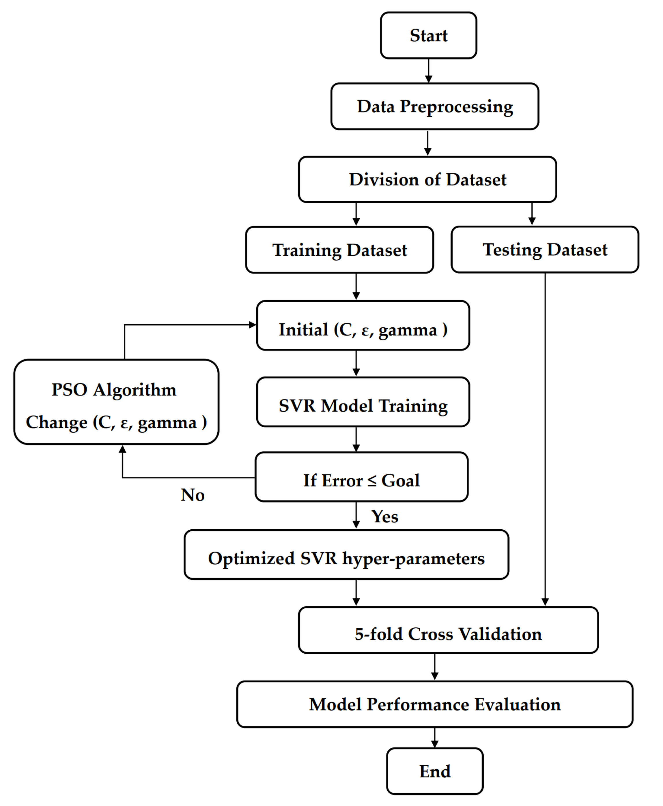
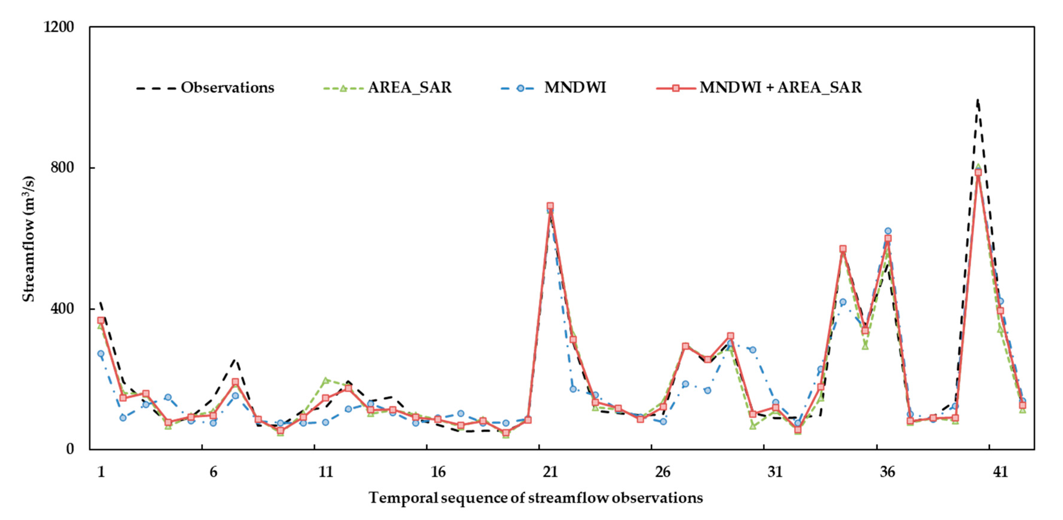
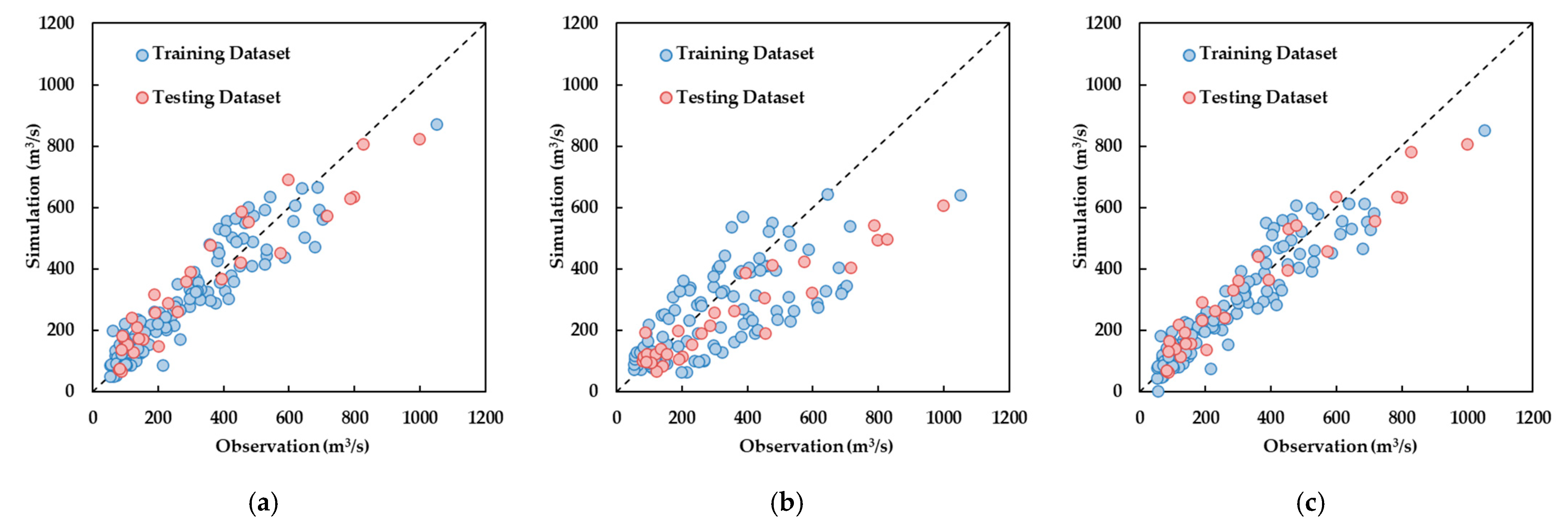
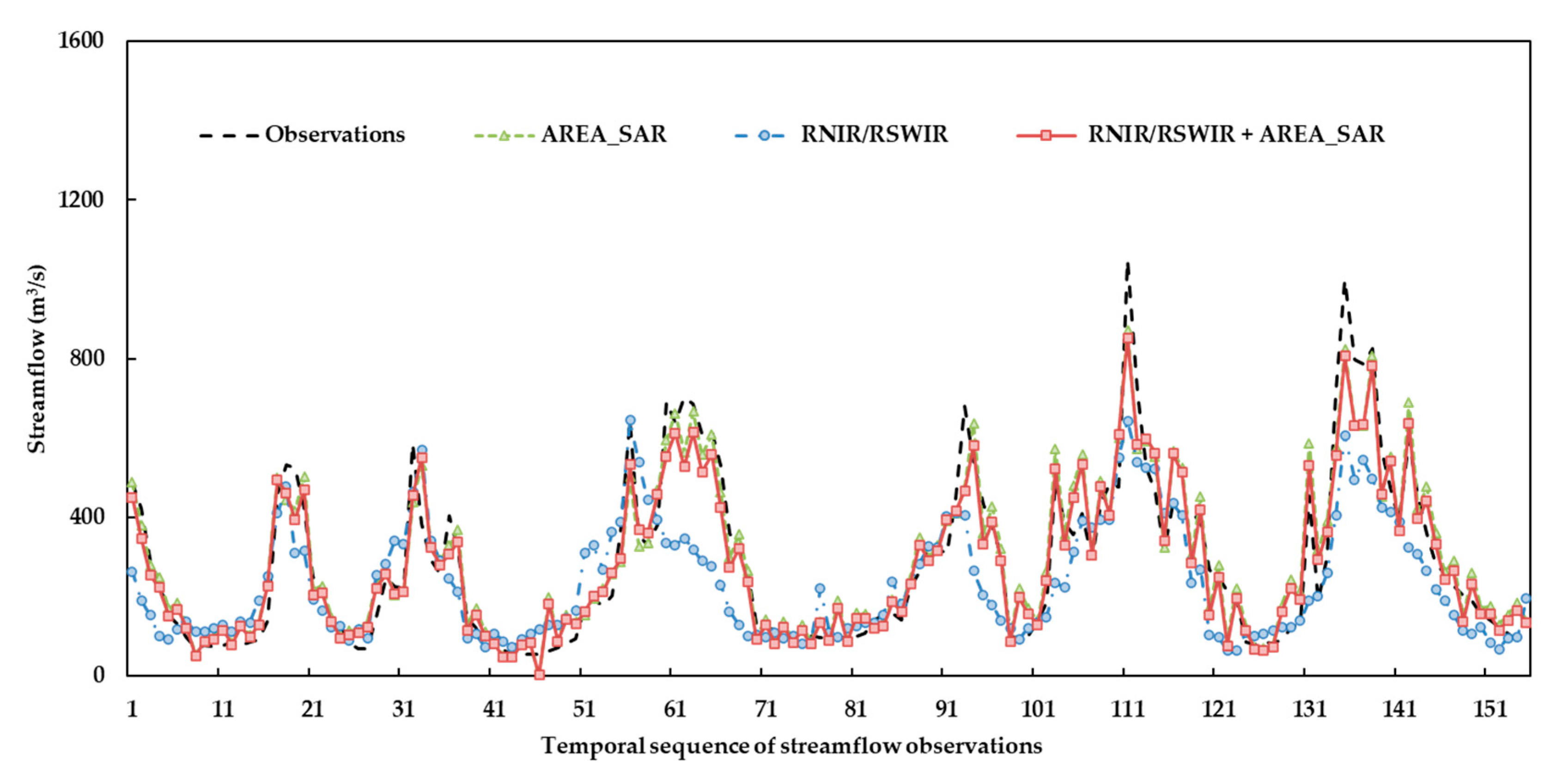
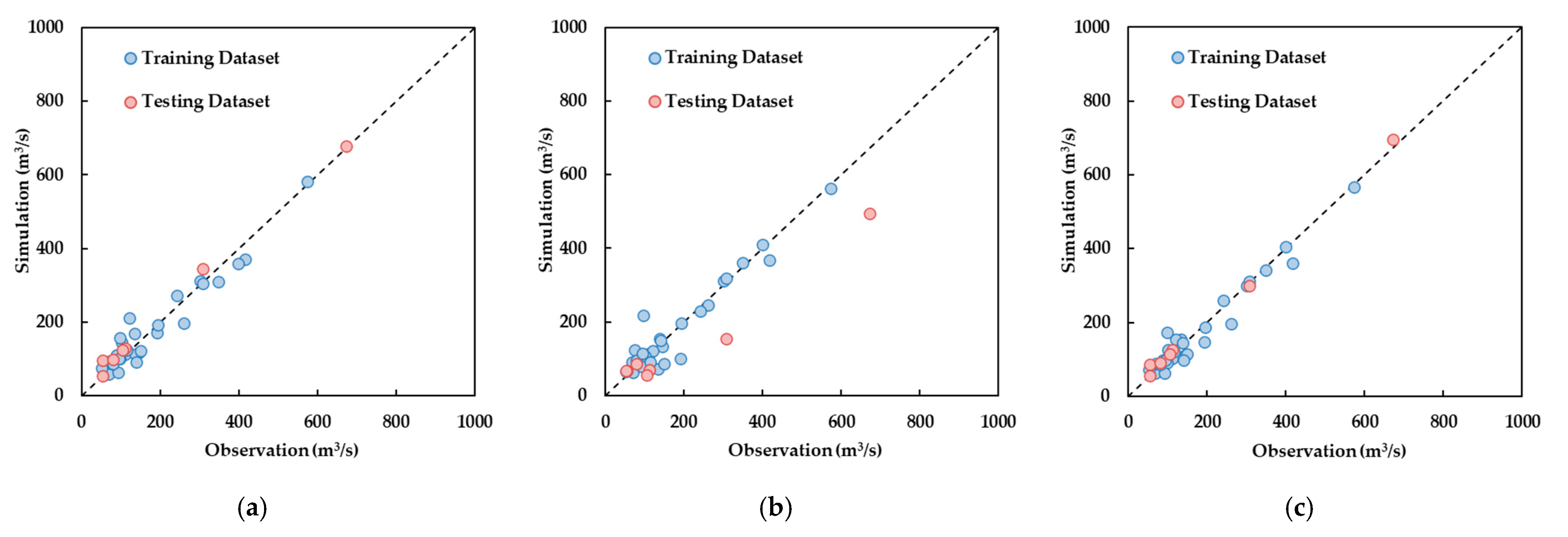
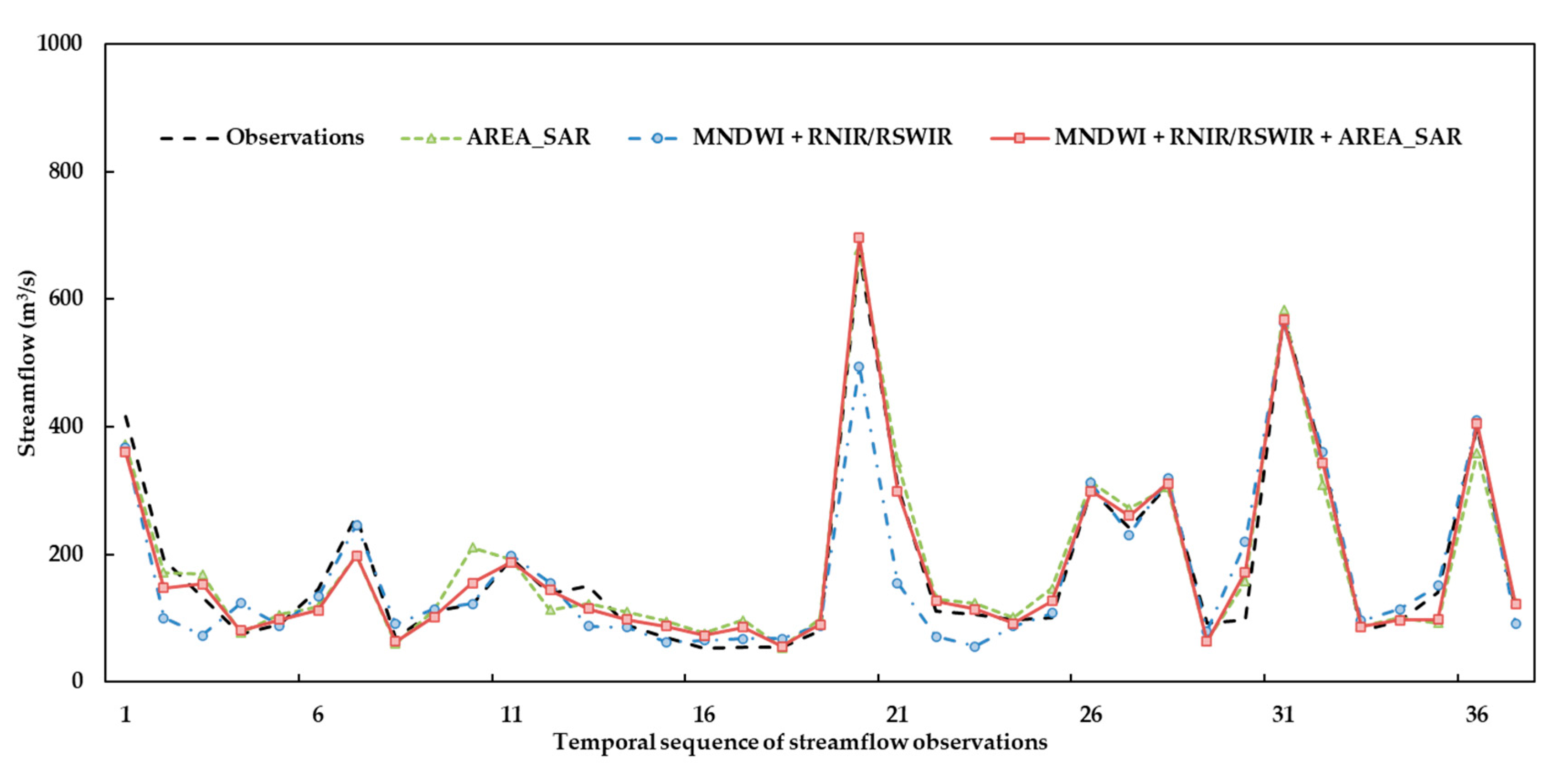
In this study, a method to merge information about water extracted from different optical (i.e., Landsat and MODIS) and SAR (i.e., Sentinel-1) satellite sensors was developed, using the SVR algorithm for streamflow estimation. The river segment upstream of the Ganzi gauging station of Yalong River, a typical river in the Qinghai–Tibetan region, was taken as a proof of concept to investigate the applicability and potential of the proposed method. Three experiments were designed to demonstrate the feasibility of using different combinations of satellite observations. In each experiment, the performance values of three developed models were compared. In Experiment I, the MRE and MAE of streamflow estimates corresponding to the SVR model using both AREA_SAR and MNDWI were 0.19 and 31.6 m³/s for the testing dataset, respectively, and were lower than the two models using AREA_SAR or MNDWI solely as inputs. In Experiment II, the MRE and MAE for the model using R_NIR/R_SWIR and AREA_SAR were 0.25 and 56.5 m³/s, respectively, and outperformed the two models treating AREA_SAR or MNDWI as single types of input. In Experiment III, the model combining all three types of satellite observations exhibited the highest accuracy, for which the MRE and MAE were 0.18 and 18.4 m³/s, respectively. The results from all three experiments demonstrated that, for the studied river segment, combined observations from optical and radar sensors can provide more accurate streamflow estimates than using a single type of seniors. For a single model, estimates for the high-flow period performed better than those for the low-flow period. In conclusion, the proposed method has great potential for the near-real-time estimation of flood magnitude or the reconstruction of variations in streamflow using historical satellite images in data-sparse regions. To further evaluate its applicability, testing the method in more rivers with different morphological and climatic conditions would be indispensable.

References

1. Robert Brakenridge, G.; Cohen, S.; Kettner, A.J.; De Groeve, T.; Nghiem, S.V.; Syvitski, J.P.M.; Fekete, B.M. Calibration of satellite measurements of river discharge using a global hydrology model. J. Hydrol. 2012, 475, 123–136. [Google Scholar] [CrossRef]
2. Blythe, T.L.; Schmidt, J.C. Estimating the Natural Flow Regime of Rivers with Long-Standing Development: The Northern Branch of the Rio Grande. Water Resour. Res. 2018, 54, 1212–1236. [Google Scholar] [CrossRef]
3. Bjerklie, D.M.; Lawrence Dingman, S.; Vorosmarty, C.J.; Bolster, C.H.; Congalton, R.G. Evaluating the potential for measuring river discharge from space. J. Hydrol. 2003, 278, 17–38. [Google Scholar] [CrossRef]
4. Hossain, F.; Siddique-E-Akbor, A.H.; Mazumder, L.C.; ShahNewaz, S.M.; Biancamaria, S.; Lee, H.; Shum, C.K. Proof of Concept of an Altimeter-Based River Forecasting System for Transboundary Flow Inside Bangladesh. IEEE J.-Stars. 2014, 7, 587–601. [Google Scholar] [CrossRef]
5. Biancamaria, S.; Hossain, F.; Lettenmaier, D.P. Forecasting transboundary river water elevations from space. Geophys. Res. Lett. 2011, 38. [Google Scholar] [CrossRef]
6. Tourian, M.J.; Tarpanelli, A.; Elmi, O.; Qin, T.; Brocca, L.; Moramarco, T.; Sneeuw, N. Spatiotemporal densification of river water level time series by multimission satellite altimetry. Water Resour. Res. 2016, 52, 1140–1159. [Google Scholar] [CrossRef]
7. Parajka, J.; Merz, R.; Blöschl, G. A comparison of regionalisation methods for catchment model parameters. Hydrol. Earth Syst. Sci. 2005, 9, 157–171. [Google Scholar] [CrossRef]
8. Garambois, P.; Monnier, J. Inference of effective river properties from remotely sensed observations of water surface. Adv. Water Resour. 2015, 79, 103–120. [Google Scholar] [CrossRef]
9. Gleason, C.J.; Smith, L.C.; Lee, J. Retrieval of river discharge solely from satellite imagery and at-many-stations hydraulic geometry: Sensitivity to river form and optimization parameters. Water Resour. Res. 2014, 50, 9604–9619. [Google Scholar] [CrossRef]
10. Huang, Q.; Long, D.; Du, M.; Zeng, C.; Li, X.; Hou, A.; Hong, Y. An improved approach to monitoring Brahmaputra River water levels using retracked altimetry data. Remote Sens. Environ. 2018, 211, 112–128. [Google Scholar] [CrossRef]
11. Getirana, A.C.V. Integrating spatial altimetry data into the automatic calibration of hydrological models. J. Hydrol. 2010, 387, 244–255. [Google Scholar] [CrossRef]
12. Leon, J.G.; Calmant, S.; Seyler, F.; Bonnet, M.P.; Cauhopé, M.; Frappart, F.; Filizola, N.; Fraizy, P. Rating curves and estimation of average water depth at the upper Negro River based on satellite altimeter data and modeled discharges. J. Hydrol. 2006, 328, 481–496. [Google Scholar] [CrossRef]
13. Sun, W.; Ishidaira, H.; Bastola, S. Calibration of hydrological models in ungauged basins based on satellite radar altimetry observations of river water level. Hydrol. Process. 2012, 26, 3524–3537. [Google Scholar] [CrossRef]
14. Kouraev, A.V.; Zakharova, E.A.; Samain, O.; Mognard, N.M.; Cazenave, A. Ob’ river discharge from TOPEX/Poseidon satellite altimetry (1992–2002). Remote Sens. Environ. 2004, 93, 238–245. [Google Scholar] [CrossRef]
15. Papa, F.; Durand, F.; Rossow, W.B.; Rahman, A.; Bala, S.K. Satellite altimeter-derived monthly discharge of the Ganga-Brahmaputra River and its seasonal to interannual variations from 1993 to 2008. J. Geophys. Res. Ocean. 2010, 115. [Google Scholar] [CrossRef]
16. Huang, Q.; Long, D.; Du, M.; Han, Z.; Han, P. Daily Continuous River Discharge Estimation for Ungauged Basins Using a Hydrologic Model Calibrated by Satellite Altimetry: Implications for theSWOT Mission. Water Resour. Res. 2020, 56, e2020WR027309. [Google Scholar] [CrossRef]
17. Tarpanelli, A.; Santi, E.; Tourian, M.J.; Filippucci, P.; Amarnath, G.; Brocca, L. Daily River Discharge Estimates by Merging Satellite Optical Sensors and Radar Altimetry Through Artificial Neural Network. IEEE Trans. Geosci. Remote. 2019, 57, 329–341. [Google Scholar] [CrossRef]
18. Bonnema, M.; Hossain, F. Assessing the Potential of the Surface Water and Ocean Topography Mission for Reservoir Monitoring in the Mekong River Basin. Water Resour. Res. 2019, 55, 444–461. [Google Scholar] [CrossRef]
19. Williams, D.L.; Goward, S.; Arvidson, Trans. Landsat: Yesterday, today, and tomorrow. Photogramm. Eng. Rem. S. 2006, 72, 1171–1178. [Google Scholar] [CrossRef]
20. Tan, Z.; Melack, J.; Li, Y.; Liu, X.; Chen, B.; Zhang, Q. Estimation of water volume in ungauged, dynamic floodplain lakes. Environ. Res. Lett. 2020, 15, 54021. [Google Scholar] [CrossRef]
21. Smith, L.C.; Isacks, B.L.; Forster, R.R.; Bloom, A.L.; Preuss, I. Estimation of discharge from braided glacial rivers using ERS 1 synthetic aperture radar: First results. Water Resour. Res. 1995, 31, 1325–1329. [Google Scholar] [CrossRef]
22. Huang, Q.; Long, D.; Du, M.; Zeng, C.; Qiao, G.; Li, X.; Hou, A.; Hong, Y. Discharge estimation in high-mountain regions with improved methods using multisource remote sensing: A case study of the Upper Brahmaputra River. Remote Sens. Environ. 2018, 219, 115–134. [Google Scholar] [CrossRef]
23. Xiang, Z.; Yan, J.; Demir, I. A Rainfall-Runoff Model with LSTM-Based Sequence-to-Sequence Learning. Water Resour. Res. 2020, 56, e2019WR025326. [Google Scholar] [CrossRef]
24. Adnan, R.M.; Liang, Z.; Heddam, S.; Zounemat-Kermani, M.; Kisi, O.; Li, B. Least square support vector machine and multivariate adaptive regression splines for streamflow prediction in mountainous basin using hydro-meteorological data as inputs. J. Hydrol. 2020, 586, 124371. [Google Scholar] [CrossRef]
25. Band, S.S.; Janizadeh, S.; Chandra Pal, S.; Saha, A.; Chakrabortty, R.; Melesse, A.M.; Mosavi, A. Flash Flood Susceptibility Modeling Using New Approaches of Hybrid and Ensemble Tree-Based Machine Learning Algorithms. Remote Sens. 2020, 12, 3568. [Google Scholar] [CrossRef]
26. Aziz, A.; Essam, Y.; Ahmed, A.N.; Huang, Y.F.; El-Shafie, A. An assessment of sedimentation in Terengganu River, Malaysia using satellite imagery. Ain Shams Eng. J. 2021, 12, 3429–3438. [Google Scholar] [CrossRef]
27. Sahoo, D.P.; Sahoo, B.; Tiwari, M.K.; Behera, G.K. Integrated remote sensing and machine learning tools for estimating ecological flow regimes in tropical river reaches. J. Environ. Manage. 2022, 322, 116121. [Google Scholar] [CrossRef]
28. Zaji, A.H.; Bonakdari, H.; Gharabaghi, B. Applying Upstream Satellite Signals and a 2-D Error Minimization Algorithm to Advance Early Warning and Management of Flood Water Levels and River Discharge. IEEE Trans. Geosci. Remote. 2019, 57, 902–910. [Google Scholar] [CrossRef]
29. Google Earth Engine. Sentinel-1 SAR GRD: C-band Synthetic Aperture Radar Ground Range Detected; ESA: Noordwijk, The Netherlands, 2019. [Google Scholar]
30. Lee, J.; Grunes, M.R.; de Grandi, G. Polarimetric SAR speckle filtering and its implication for classification. IEEE Trans. Geosci. Remote. 1999, 37, 2363–2373. [Google Scholar]
31. Xu, H. Modification of normalised difference water index (NDWI) to enhance open water features in remotely sensed imagery. Int. J. Remote Sens. 2006, 27, 3025–3033. [Google Scholar] [CrossRef]
32. Li, S.; Sun, D.; Yu, Y.; Csiszar, I.; Stefanidis, A.; Goldberg, M.D. A New Short-Wave Infrared (SWIR) Method for Quantitative Water Fraction Derivation and Evaluation with EOS/MODIS and Landsat/TM Data. IEEE Trans. Geosci. Remote. 2013, 51, 1852–1862. [Google Scholar] [CrossRef]
33. Otsu, N. A Threshold Selection Method from Gray-Level Histograms. IEEE Trans. Syst. Man Cybern. 1979, 9, 62–66. [Google Scholar] [CrossRef]
34. Lin, J.; Cheng, C.; Chau, K. Using support vector machines for long-term discharge prediction. Hydrol. Sci. J. 2006, 51, 599–612. [Google Scholar] [CrossRef]
35. Ng, K.W.; Huang, Y.F.; Koo, C.H.; Chong, K.L.; El-Shafie, A.; Najah Ahmed, A. A review of hybrid deep learning applications for streamflow forecasting. J. Hydrol. 2023, 625, 130141. [Google Scholar] [CrossRef]
36. Tripathi, S.; Srinivas, V.V.; Nanjundiah, R.S. Downscaling of precipitation for climate change scenarios: A support vector machine approach. J. Hydrol. 2006, 330, 621–640. [Google Scholar] [CrossRef]
37. Vapnik, V.N. The Nature of Statistical Learning Theory; Springer: New York, NY, USA, 1995. [Google Scholar]
38. Kenedy, J.; Eberheart, R. Particle Swarm Optimization. In Proceedings of the IEEE International Conference on Neural Networks, Perth, WA, Australia, 27 November–1 December 1995; Volume 4, pp. 1942–1948. [Google Scholar]
39. Pham, Q.B.; Kumar, M.; Di Nunno, F.; Elbeltagi, A.; Granata, F.; Islam, A.R.M.T.; Talukdar, S.; Nguyen, X.C.; Ahmed, A.N.; Anh, D.T. Groundwater level prediction using machine learning algorithms in a drought-prone area. Neural Comput. Appl. 2022, 34, 10751–10773. [Google Scholar] [CrossRef]
40. Rahaman, M.H.; Roshani; Masroor, M.; Sajjad, H. Integrating remote sensing derived indices and machine learning algorithms for precise extraction of small surface water bodies in the lower Thoubal river watershed, India. J. Clean. Prod. 2023, 422, 138563. [Google Scholar] [CrossRef]
41. Seyoum, W.M.; Kwon, D. Suitability of satellite-based hydro-climate variables and machine learning for streamflow modeling at various scale watersheds. Hydrol. Sci. J. 2020, 65, 2233–2248. [Google Scholar] [CrossRef]
42. Ni, L.; Wang, D.; Singh, V.P.; Wu, J.; Wang, Y.; Tao, Y.; Zhang, J. Streamflow and rainfall forecasting by two long short-term memory-based models. J. Hydrol. 2020, 583, 124296. [Google Scholar] [CrossRef]
43. Uysal, G.; Şensoy, A.; Şorman, A.A. Improving daily streamflow forecasts in mountainous Upper Euphrates basin by multi-layer perceptron model with satellite snow products. J. Hydrol. 2016, 543, 630–650. [Google Scholar] [CrossRef]
44. Deng, H.; Chen, W.; Huang, G. Deep insight into daily runoff forecasting based on a CNN-LSTM model. Nat. Hazards. 2022, 113, 1675–1696. [Google Scholar] [CrossRef]
45. Cho, K.; Kim, Y. Improving streamflow prediction in the WRF-Hydro model with LSTM networks. J. Hydrol. 2022, 605, 127297. [Google Scholar] [CrossRef]
46. Hochreiter, S.; Schmidhuber, J. Long Short-Term Memory. Neural Comput. 1997, 9, 1735–1780. [Google Scholar] [CrossRef] [PubMed]
47. Xiong, J.; Guo, S.; Yin, J. Discharge Estimation Using Integrated Satellite Data and Hybrid Model in the Midstream Yangtze River. Remote Sens. 2021, 13, 2272. [Google Scholar] [CrossRef]
48. García-Pintado, J.; Mason, D.C.; Dance, S.L.; Cloke, H.L.; Neal, J.C.; Freer, J.; Bates, P.D. Satellite-supported flood forecasting in river networks: A real case study. J. Hydrol. 2015, 523, 706–724. [Google Scholar] [CrossRef]
49. Ishitsuka, Y.; Gleason, C.J.; Hagemann, M.W.; Beighley, E.; Allen, G.H.; Feng, D.; Lin, P.; Pan, M.; Andreadis, K.; Pavelsky, T.M. Combining Optical Remote Sensing, McFLI Discharge Estimation, Global Hydrologic Modeling, and Data Assimilation to Improve Daily Discharge Estimates Across an Entire Large Watershed. Water Resour. Res. 2021, 57, e2020WR027794. [Google Scholar] [CrossRef]
Figure 1. Upstream region of the Yalong River Basin and its location in the Yangtze River Basin.
Remotesensing 15 05184 g001
Figure 2. The river segment upstream of Ganzi station, with a length of 13.8 km, is shown in red. The red star indicates the location of Ganzi station.
Remotesensing 15 05184 g002
Figure 3. Methodological flowchart for streamflow estimation in this study.
Remotesensing 15 05184 g003
Figure 4. Scatterplots of the observed and simulated streamflows by Experiment I with different input combinations: (a) AREA_SAR; (b) MNDWI; and (c) MNDWI + AREA_SAR.
Remotesensing 15 05184 g004
Figure 5. Time-variation hydrographs of the observations and simulations by Experiment I with different input combinations: AREA_SAR (Model 1); MNDWI (Model 2); AREA_SAR+MNDWI (Model 3).
Remotesensing 15 05184 g005
Figure 6. Scatterplots of the observed and simulated streamflows by Experiment II with different input combinations: (a) AREA_SAR; (b) RNIR/RSWIR; and (c) RNIR/RSWIR + AREA_SAR.
Remotesensing 15 05184 g006
Figure 7. Time-variation hydrographs of the observations and simulations by Experiment II with different input combinations: AREA_SAR (Model 4); RNIR/RSWIR (Model 5); AREA_SAR + RNIR/RSWIR (Model 6).
Remotesensing 15 05184 g007
Figure 8. Scatterplots of the observed and simulated streamflows by Experiment III with different input combinations: (a) AREA_SAR; (b) MNDWI + RNIR/RSWIR; and (c) MNDWI + RNIR/RSWIR + AREA_SAR.
Remotesensing 15 05184 g008
Figure 9. Time-variation hydrographs of the observed and simulated streamflows by Experiment III with different input combinations: AREA_SAR (Model 7); MNDWI + RNIR/RSWIR (Model 8); MNDWI + RNIR/RSWIR + AREA_SAR (Model 9).
Remotesensing 15 05184 g009