Article

Influence of Flight Altitude and Surface Characteristics on UAS-LiDAR Ground Height Estimate Accuracy in Juncus roemerianus Scheele-Dominated Marshes

by
Michael Amelunke
1,*,
Carlton P. Anderson
1,
Margaret C. B. Waldron
1,2,
George T. Raber
1,3 and
Gregory A. Carter
1,3,4
1
Gulf Coast Geospatial Center, University of Southern Mississippi, Long Beach, MS 39560, USA
2
School of Ocean Science and Engineering, University of Southern Mississippi, Long Beach, MS 39560, USA
3
School of Biological, Environmental, and Earth Sciences, University of Southern Mississippi, Hattiesburg, MS 39406, USA
4
School of Coastal Resilience, University of Southern Mississippi, Long Beach, MS 39560, USA
*
Author to whom correspondence should be addressed.
Remote Sens. 2024, 16(2), 384; https://doi.org/10.3390/rs16020384
Submission received: 6 November 2023 / Revised: 13 January 2024 / Accepted: 15 January 2024 / Published: 18 January 2024
(This article belongs to the Section Remote Sensing in Geology, Geomorphology and Hydrology)

Abstract

:
Management and monitoring of vulnerable coastal marshes rely on accurate ground height estimates. However, marsh surface characteristics such as vegetation and water presence complicate aerial remote sensing of the ground. Towards developing an improved understanding and techniques for these remote sensing efforts, this study established relationships among data collection flight altitude, surface characteristics, and ground height estimate accuracy within Juncus roemerianus Scheele-dominated marshes. Uncrewed Aerial System (UAS) Light Detection and Ranging (LiDAR) sampling was conducted at five altitudes for five marsh sites and one local control site. Survey-grade topographic measurements and marsh surface characteristics were recorded at each site for comparison. Root Mean Square Error (RMSE) and linear mixed-effects modeling were used to quantify relationships among vertical error, altitude, and surface characteristics. For low (24–72 m) and high (96–120 m) altitudes Above Ground Level (AGL), the RMSE values were 49 cm and 17 cm, respectively. Despite this appreciable improvement in accuracy with increasing flight altitude, point density values of these datasets limit applications. Linear mixed-effects modeling further emphasized the complex relationships between sensor footprint size, surface characteristics, and ground height estimates. These findings have direct implications for elevation modeling and monitoring efforts of frequently inundated, coastal marshes.

1. Introduction

Environmental monitoring and habitat mapping of coastal marshes are increasingly relied upon to characterize changes in marsh areal extent and vulnerability of plant communities over time. These efforts are important because of the critical ecosystem services which marsh plant communities provide, such as buffering from storm surge and wave energy [1,2,3], providing habitat for coastal wildlife, sequestering atmospheric and organic carbon [4,5], and mitigating land subsidence and loss through sediment capture [6,7]. Given the sensitivity of coastal marsh to sea level rise and subsidence, understanding change in marsh surface height is an important component of marsh monitoring [8,9]. Passive remote sensing methods for determining marsh ground surface height such as Structure from Motion (SfM) are commonly applied in vegetated environments, but with limited success [10,11,12,13,14]. Dense, tall, and homogenous vegetation existing on marsh platforms creates challenges for the automated photogrammetric methods implemented in software, often leading to overestimations of ground surface height [13,15]. For these passive methods, densely vegetated environments with limited visible, rigid structures are often more conducive to the generation of Digital Surface Models (DSMs) representing the canopy surface rather than Digital Terrain Models (DTMs) which represent the ground surface [12,13,14]. Alternatively, aerial LiDAR is recognized as having greater canopy-penetrating capabilities than aerial photogrammetry [12,15,16] and can be operated over much larger areas than in situ field surveys.
The determination of ground height in coastal marsh environments using LiDAR also presents unique problems [17,18,19,20]. Coastal marshes are characterized by homogenous, dense canopies [21]. When the ground is covered by vegetation, discrete return and full waveform LiDAR sensors can record multiple height estimates per outgoing pulse. However, discrete return LiDAR systems often cannot record separate vegetation surface returns and near-ground returns in short, dense canopies [22,23,24,25]. In taller canopies, LiDAR systems may record multiple returns, but these returns are predominantly from upper and mid-canopy heights [19,20,22]. LiDAR pulses that penetrate the marsh canopy to the underlying terrain often encounter standing water. This can inhibit the pulse from returning to the sensor, as many LiDAR systems operate using a near-infrared wavelength that is significantly absorbed by water. Canopy height, stem density, leaf structure and orientation, growth habit, and other canopy characteristics also affect LiDAR pulses [20,22,25].
When compared to UASs, LiDAR sensors flown on crewed aircraft operate at high altitudes, resulting in relatively large laser footprints on the ground and thus lower point densities relative to UAS LiDAR systems. However, flight time and coverage are much higher for crewed aircraft. By contrast, UAS LiDAR systems can potentially resolve smaller topographic features [26]. UAS platforms can also be more feasible to operate at a fine temporal resolution and are more rapidly deployable because of their lower operational cost and accessibility [27,28]. Furthermore, with pre-programmed flight plans, repeat surveying of the same area is simplified [29].
Very few studies have assessed the accuracy of UAS LiDAR systems in measuring ground height in coastal marshes [15,30]. In comparing UAS LiDAR and photogrammetry in a marsh dominated by Spartina alterniflora Loisel (Smooth Cordgrass), Pinton et al. (2021) [15] found that LiDAR yielded more accurate ground heights versus UAS photogrammetry and suggested that future efforts should investigate how the discrepancy may be influenced by flight altitude [15]. In a Spanish coastal marsh, Curcio et al. (2022) [30] compared the efficacy of UAS LiDAR in determining ground height from two altitudes and varied sensor scanning configurations. They found that a lower flight altitude of 60 m slightly decreased RMSE values from those at 100 m and measurement reliability was increased with increasing point cloud density [30]. Although the effects of altitude on ground height estimate uncertainty within densely vegetated marsh settings was demonstrated by the aforementioned study, relationships among flight altitude and marsh surface characteristics such as canopy height and structure, plant species, and water depth should be explored further. Understanding these relationships will help guide future data collection efforts.
Because of the widespread dominance of S. alterniflora along the Atlantic and parts of the Gulf of Mexico coast, more research focus has been placed on quantifying ground height estimate uncertainty in marshes dominated by S. alterniflora marshes than those dominated by J. roemerianus [15,20,22,23,31,32]. Along the Mississippi Gulf Coast, USA, J. roemerianus-dominated marshes comprise approximately 96% of the mainland marsh area, making this an important species for research [33]. Medeiros et al. (2015), Hladik and Alber (2012), and Schmid et al. (2011) describe similar inaccuracies associated with Juncus roemerianus Scheele (Black Needlerush) when investigating airplane-mounted LiDAR systems [22,25,34]. However, the effects of J. roemerianus on ground height estimate error have been studied considerably less [22]. Establishing a more detailed understanding of marsh ground height estimates in these areas is an important contribution to the current body of related research, and, more specifically, provides an important baseline for future research along the Mississippi Gulf Coast.
Herein, we assess the accuracy of UAS LiDAR-derived ground height estimates in a J. roemerianus-dominated coastal marsh setting, comparing and incorporating data from a control site and using a novel ground classification technique. The primary goal of this study was to examine the relationships among UAS LiDAR ground height estimate accuracy, flight altitude, and surface characteristics in these marsh settings. Five sites from within Mississippi’s Coastal Preserves and one control site for comparison were surveyed. UAS LiDAR data were collected along a sampling transect at each of the sites at five different altitudes. Topographic field surveys were conducted along the same transects to record precise ground elevation, and site characteristics including water depth, canopy height, and canopy orientation to assess these relationships with LiDAR measurement accuracy. Results indicate that altitude and marsh surface characteristics both impact LiDAR ground height estimates within J. roemerianus-dominated coastal marshes. The relationships established here highlight key areas for future, pertinent research towards mitigating ground height estimate error in airborne LiDAR datasets.

2. Materials and Methods

To evaluate accuracy of UAS LiDAR-derived marsh ground height estimates, five different J. roemerianus marsh transects were surveyed using UAS LiDAR and an on-the-ground, rod-mounted, Global Navigation Satellite System (GNSS) roving receiver. Additionally, a control transect over asphalt and mowed grass was surveyed six times during the study to assess sensor performance. LiDAR flights were conducted at five altitudes at each site. Altitude-based correction factors were derived based on the control site. The GNSS field survey was conducted at 1 m intervals along each transect and included measurements of canopy height and water depth. Any unique site characteristics (e.g., flattened canopy, sparse canopy, presence of water channels, etc.) were recorded. After heights were corrected for flight altitude, point cloud datasets were classified using a novel ground estimation method. Finally, vertical accuracy was assessed by computing the Root Mean Squared Error, RMSE, of these LiDAR heights compared with the corresponding GNSS heights for both the classified and unclassified datasets. The major steps conducted in the methodology of this study are displayed in Figure 1.

2.1. Site Selection

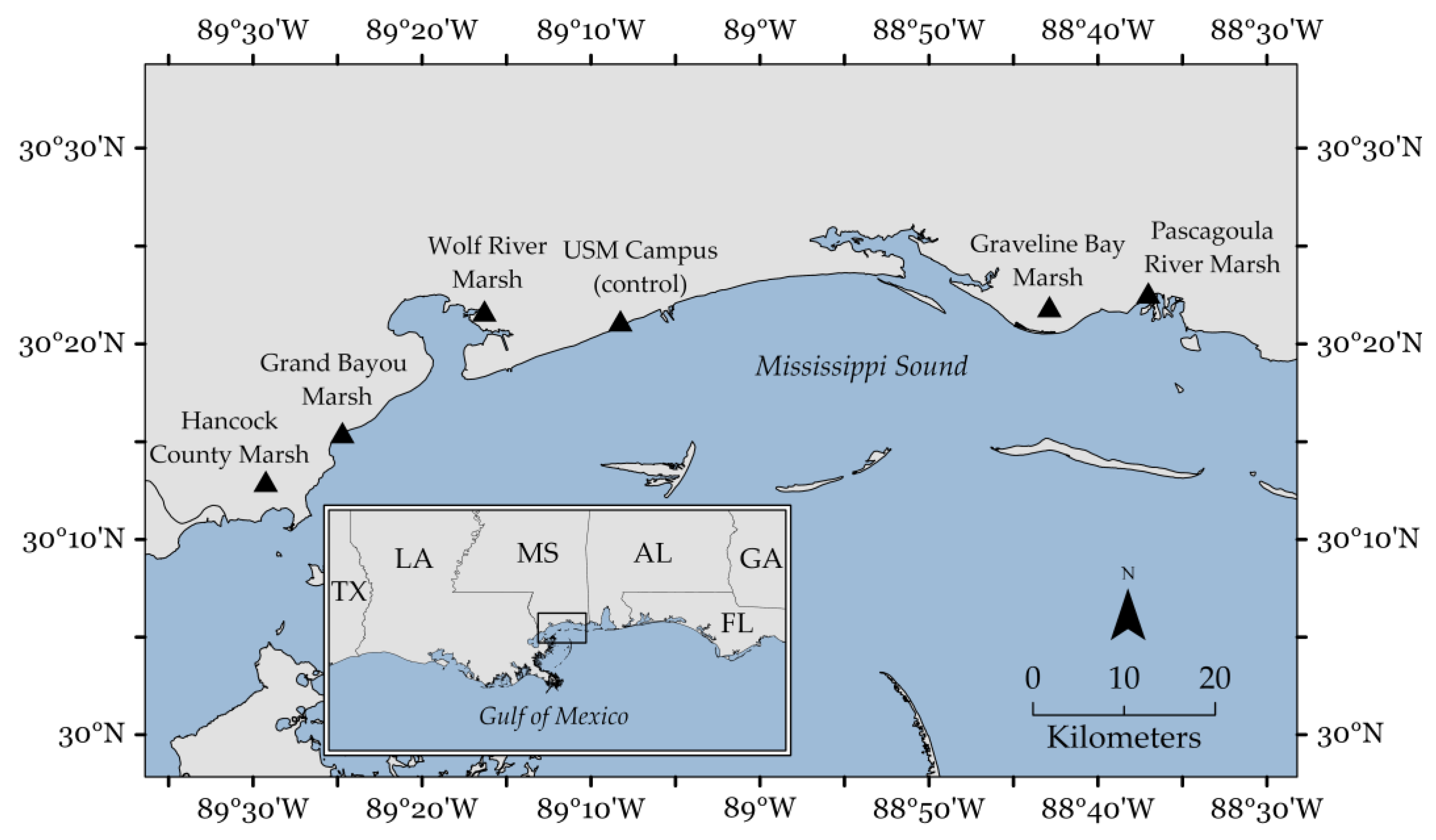
The locations of the J. roemerianus-dominated marsh sites that were selected for study from within five Mississippi Coastal Preserves, along with one control site established at the University of Southern Mississippi (USM) Gulf Park Campus are shown in Figure 2. The Mississippi Coastal Preserves consist of approximately 16,000 ha of protected estuarine area spanning Mississippi’s coastline [35]. Sites were selected from within the Hancock County, Grand Bayou, Wolf River, Graveline Bay, and Pascagoula River Marsh Preserves. All sites were restricted to general airspace as designated by the Federal Aviation Administration (FAA). Sites were required to be accessible by road, traversable by foot for ground surveys, and dominated by homogenous stands of J. roemerianus (Figure 3). Within each preserve, a 60 m sampling transect perpendicular to the adjacent upland/marsh transition was established. Minimal adjustments to the orientation and the start of the transect were made when necessary to ensure J. roemerianus dominance along the transect and to avoid tidal rivulets and creeks that could not be easily traversed. The on-campus control site consisted of a 60 m transect that spanned 40 m of sparsely vegetated, mowed grass and 20 m of an adjacent asphalt parking lot. This site was included to assess the ground height estimate accuracy of the UAS LiDAR sensor in comparison with GNSS field survey measurements.

2.2. Field Data Collection

All field data from marsh sites were acquired during the 2021 and 2022 growing seasons. During this time, there were no significant tropical cyclone impacts to the study areas. LiDAR data were collected prior to ground surveys to allow data acquisition of undisturbed vegetation and soil surfaces. All positions referenced the NAD83 (2011) datum and ellipsoid.

2.2.1. UAS-LiDAR Data Collection

LiDAR data were collected using a Microdrones md4-1000 quadcopter with an attached SICK LD-MRS420201 LiDAR sensor. This sensor is a discrete return LiDAR with the capability to record three range measurements per pulse from two near-infrared (905 nm ± 10 nm) lasers scanning at a frequency of 25 Hz. The reported horizontal and vertical accuracy for this integrated platform and sensor is 6 cm when flown at 40 m AGL [36].
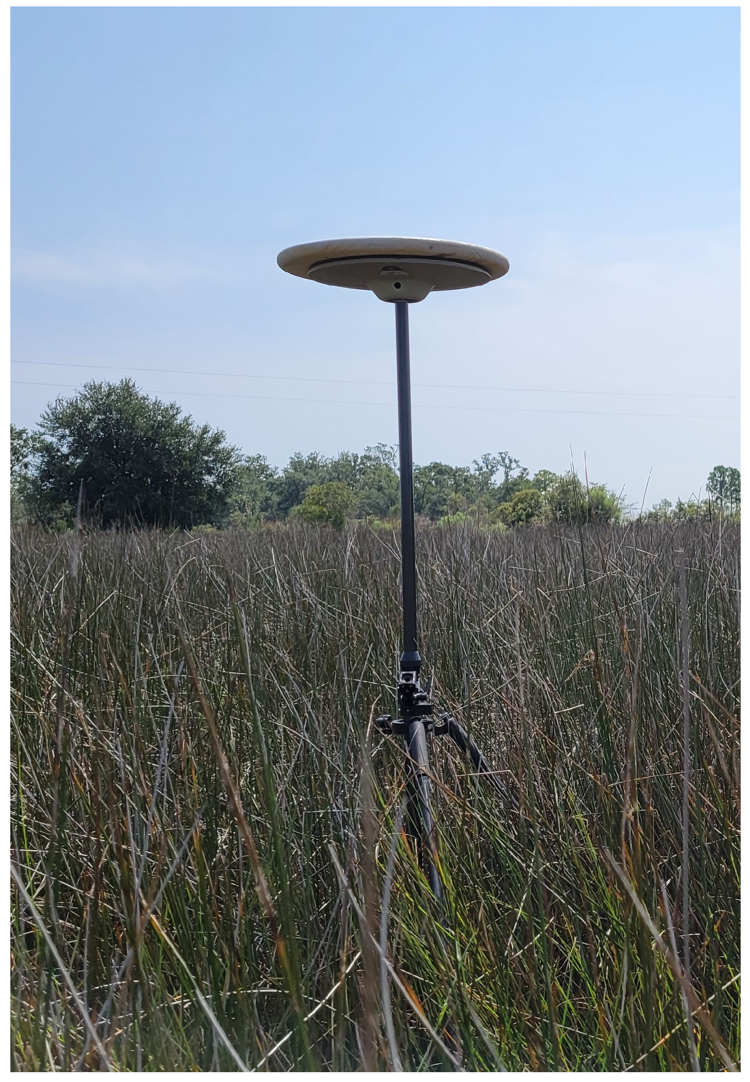
To validate the proper functioning of the LiDAR sensor for each sampling site, two control targets were placed above the marsh canopy at opposite ends of the sampling transect. The targets were positioned similarly at the control site. The control targets consisted of round, wooden plates, 0.4 m in diameter, positioned and leveled atop 2 m tall survey tripods (Figure 4). The plates were painted white to increase reflectivity and were designed after Davidson et al. (2019) [36]. The targets were highly visible in point cloud datasets due to their height above the marsh canopy and point intensity information. Five GNSS measurements were taken at the center of each control target using a Trimble R12i GNSS receiver, with positions corrected to ±2 cm accuracy using USM Gulf Coast Geospatial Center Real-Time Network (USM GCGC RTN) of GNSS Continuously Operating Reference Stations (CORS) [37]. The mean of these measurements for each target served as geodetic control for incident LiDAR returns to ensure normal sensor operation.
Along each sampling transect, LiDAR data were acquired at an approximately nadir (0°) scan angle for 5 different flight altitudes: 24 m, 48 m, 72 m, 96 m, and 120 m. These were established by dividing the maximum allowable flight altitude of 120 m (400 ft) above ground level (AGL) into five equal intervals. The flight plan consisted of a singular flight line positioned directly over the planned topographic sampling transect. Data were acquired in a single pass along the flight line. By not sampling along adjacent, overlapping flight lines, vertical error and/or canopy penetration attributed to oblique angle scanning could be separated from error due to the presence of the vegetation canopy. Flight speed and field-of-view remained constant at 2.5 m s−1 and 60°, respectively. Flights were conducted during low tide conditions to minimize the absorption and reflection of LiDAR pulses from standing water beneath vegetation canopies. LiDAR data for two of the six control site collections for 24 m were not used due to data storage failure. Due to data storage failure and UAS flight operation limitations, data for flight altitudes 72 m and 96 m at Grand Bayou, and 120 m at Graveline Bay were not completed.

2.2.2. Topographic Field Survey

Topographic sampling was performed immediately after LiDAR collection at all sites except for one (Hancock County Marsh Preserve) in which field sampling was conducted 13 days later. However, there were no documented storm disturbances to the vegetation canopy during this period and ground collection was performed under similar tidal conditions as during the LiDAR data collection. Ground height estimates were acquired using a Trimble R12i GNSS receiver with real time corrections from the GCGC RTN at 1 m spacing along a measuring tape. The receiver was attached to a 2 m survey rod with a flat topographic shoe to prevent penetration into the soft marsh soil. Site characteristics were recorded and logged at every sampling point. Plant species dominance (>50% ground coverage) and any secondary species (>25% and <50% ground coverage) were determined, and co-dominance was recorded when applicable. Additionally, canopy and water depth were measured with a leveling rod. Other relevant information related to terrain, hydrology, and canopy orientation, including incidences of flattened canopy, were also noted. LiDAR ground returns within a 0.5 m radial distance of a given topographic sample were assumed to be referencing the same ground height due to the gentle topographic gradient of the control and marsh sites.

2.3. LiDAR Processing

Initial UAS trajectory corrections were made in POSPac UAV v8.6 (Applanix software) [38]. For each flight, a 1 h GNSS data file in Receiver Independent Exchange (RINEX) 3.04 format was downloaded from the nearest GNSS CORS using the USM GCGC RTN Reference Data Shop (http://rtn.usm.edu) (accessed on 5 January 2023) [37]. LiDAR point clouds were georeferenced using mdInfinity v2020.5 [39].

2.3.1. Control Transect: LiDAR vs. GNSS Height

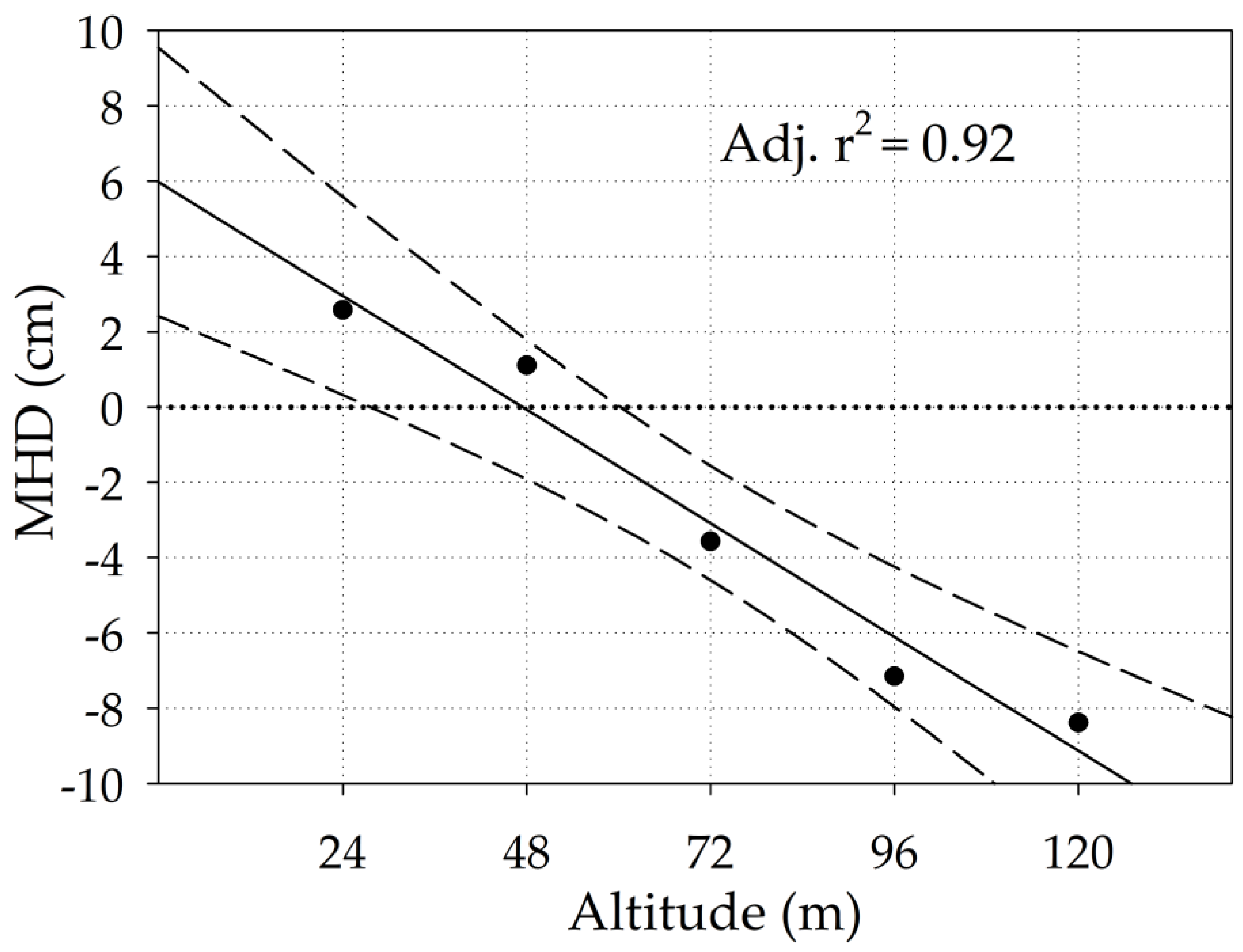
At altitudes below approximately 50 m, the LiDAR sensor consistently overestimated ground height, while underestimating ground height at altitudes above 50 m in comparison with the GNSS field survey measurements. Thus, correction factors were developed using the control site data. Due to discrepancies in the point density and intensity information between the grass and asphalt surface types, correction factors were developed using only returns from asphalt. To account for differences in height that were observed among sampling dates owing to variation in atmospheric conditions and satellite ephemeris information, six sets of control data were used for correction factor generation. To generate correction factors, all sets of control data were merged. For each altitude, 500 random LiDAR samples were taken from the asphalt portion of the transect from within a 0.5 m distance (buffer) from the GNSS field survey measurements. The height difference between the mean LiDAR height (l) and GNSS measurement height (g) was computed for LiDAR samples within each buffer. These height differences were then averaged to compute the mean height difference (MHD) for each altitude (a) using the total number of data points (N):
M H D a = i = 1 N ( l g ) N
MHD values were linearly regressed with altitude to compute a height correction factor for each altitude (Figure 5 and Table 1). These correction factors were applied to all marsh and control data prior to height accuracy evaluation.

2.3.2. Point Cloud Ground Classification

Studies evaluating the accuracy of LiDAR-derived elevation commonly use a minimum bin-gridding classification approach that classifies the lowest point within a specified grid size as ground [17,25,34,40]. This approach can lead to underestimation of true ground surfaces and preferentially select lower, erroneous points [20,25,30]. Thus, we estimated the ground points within each marsh dataset for each altitude based on a percentage of the lowest returns, with this percentage determined based on the height range of measurements obtained from the control site at the same altitude. All returns at the control site were assumed to represent true ground returns, and the variability in each control dataset compared with the topographic survey was assumed to represent variability inherent to the sensor or due to external factors such as atmospheric conditions. By contrast, the marsh sites exhibited much larger ranges due to the influence of returns from tall vegetation. At the control site and each marsh site, height ranges were calculated within a 0.5 m buffer around each sampling point along the transect for each altitude, and these height ranges were averaged to produce a single height range for each dataset at each altitude. For each altitude (a), the ratio of the average measurement height range at the control site ( r ¯ c,a) to the height range at a given marsh site at the same altitude ( r ¯ m) was used to estimate the percentage of LiDAR returns representing the ground (GP) at the marsh site:
r ¯ c , a r ¯ m , a = G P
Thus, for marsh transects with large average height ranges (areas of tall, dense vegetation), the computed percentage of ground points to use for analysis was smaller than for sites with much smaller average height ranges. This method is hereafter referred to as the Ground Percentage Estimation (GPE) method.
A Python script was developed to extract the lowest marsh ground points based on the computed ground percentage. For example, if the computed percentage of points to use for a dataset was 30%, then this script selected the lowest 30% of marsh points within each buffer to use for analysis. Preliminary testing revealed that the tool preferentially selected groupings of low-elevated points (tidal creeks, gaps in the vegetation, etc.) within each buffer rather than selecting a more even distribution of low-elevation returns. To mitigate this, each buffer was split into 4 quadrants and the computed percentage of points were selected from each of these quadrants.
To further quantify the effect of vegetation on LiDAR ground height estimate error, the GPE classified data was compared to the fully unclassified data. Although related studies have converted LiDAR point clouds into DEMs prior to accuracy assessment [17,19,25,40,41,42], we compared LiDAR point clouds from these two classification methods to high accuracy GNSS ground truth measurements to minimize potential error introduced by DEM generation [1,2].

2.4. Accuracy Evaluation

The vertical accuracy of each LiDAR data collection was validated based on the heights of returns incident upon the two control targets positioned at the beginning and end of each transect. Target returns were selected based on their height above the ground and vegetation canopy. To isolate lower intensity wooden plate returns from higher intensity returns from the metal tripod legs, an intensity threshold was set using the las2las (filter) tool in LAStools plugin for ArcGIS Pro [43]. The mean height of LiDAR returns was compared to the height of the target measured using RTN GNSS. The vertical Mean Absolute Error (MAE) was computed for each target. Values of MAE were computed as:
M A E = i = 1 N y o y p r N ,
where N is the number of data points, yo is the observed value, and ypr is the predicted value.
Root-Mean-Squared Error (RMSE) was computed between the unclassified and GPE classified datasets and the transect GNSS ground-truth measurements at each site. LiDAR returns within a 0.5 m buffer of the topographic field measurements were used for analysis. This workflow was conducted separately for the LiDAR data at each altitude. The outputs were RMSE values that represented the overall error associated with each transect for a given altitude. RMSE values were computed as:
R M S E = i = 1 N y o y p r 2 N ,
where N is the number of data points, yo is the observed value, and ypr is the predicted value.

2.5. Impacts of Surface Characteristics

A linear mixed-effects model was used to quantify the various influences of marsh surface characteristics on LiDAR ground height differences (LiDAR–GNSS). Mixed-effects models include both fixed and random effects, allowing for variability within and among hierarchical groups present in a dataset to be quantified alongside the effects of population-level variables, similar to repeated measures ANOVAs used for nested data [44]. Fixed variables are those that are expected to operate at the population level, with a predictable response of the dependent variable across various samples regardless of their hierarchical membership. Random variables are categorical grouping factors which model the hierarchical data structure and are included to quantify how samples from within each group differ from the rest of the dataset, allowing for inferences to be made about population-level fixed effects despite non-independence of the data within each hierarchical group [44]. Mixed-effects models are flexible in that they handle unbalanced designs well, allow for continuous predictors without binning, and unlike repeated measures ANOVA, provide information about the magnitude and direction of effects [44].
In our model, Site was represented as a random effect because we assume that differences are present among the sites which could not be completely captured due to limitations in our field sampling, such as stem density and leaf area index, water turbidity, and atmospheric humidity. Population-level fixed effects included in the model were Altitude, Inundation Depth, Erect Canopy Height, and Flattened Canopy Height, as well as the two-way interactions among these variables. Mixed-effects modeling was performed in R version 4.1.1 using the lme4 package [45,46]. The model was fitted using Restricted Maximum Likelihood. Significance levels of the model coefficients were evaluated using the Kenward–Roger approximation for degrees of freedom [47].

3. Results

3.1. Accuracy Evaluation

For target observations at the control site, MAE values did not exceed 8 cm at any altitude once altitude-based correction factors were applied. For the five marsh observations, these did not exceed 7 cm, indicating that the LiDAR system was operating as expected throughout the duration of this study.
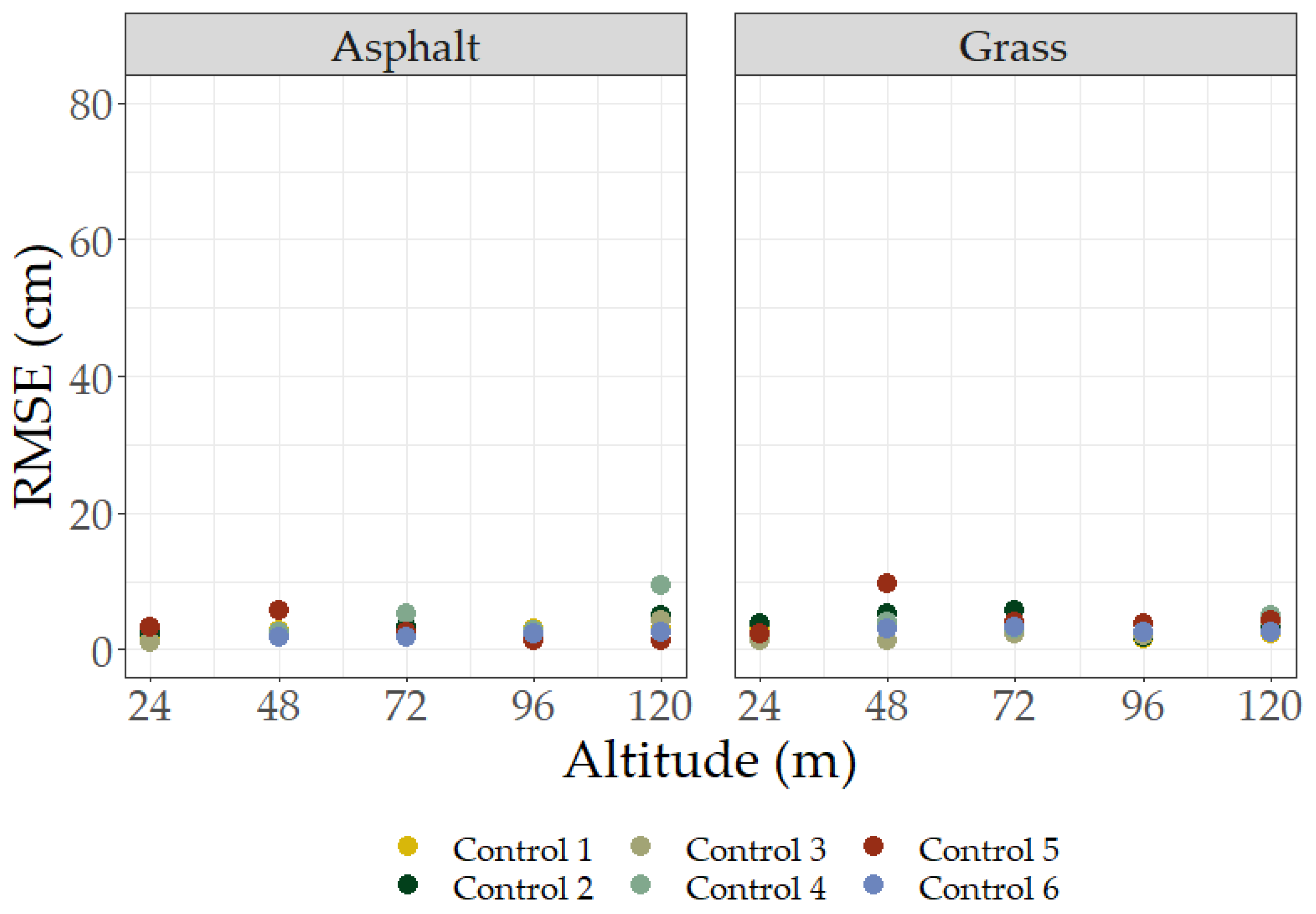
For the control site transect, there was no significant relationship between altitude and RMSE (Figure 6). RMSE values of these data ranged from 1 cm to approximately 10 cm. There was no consistent difference in RMSE between grass and asphalt surfaces. For the marsh site transects, RMSE decreased with increases in altitude (Figure 7). Unclassified data had higher RMSE values than GPE classified data for the lower altitudes and then shared the same RMSE value for the altitudes of 96 and 120 m.
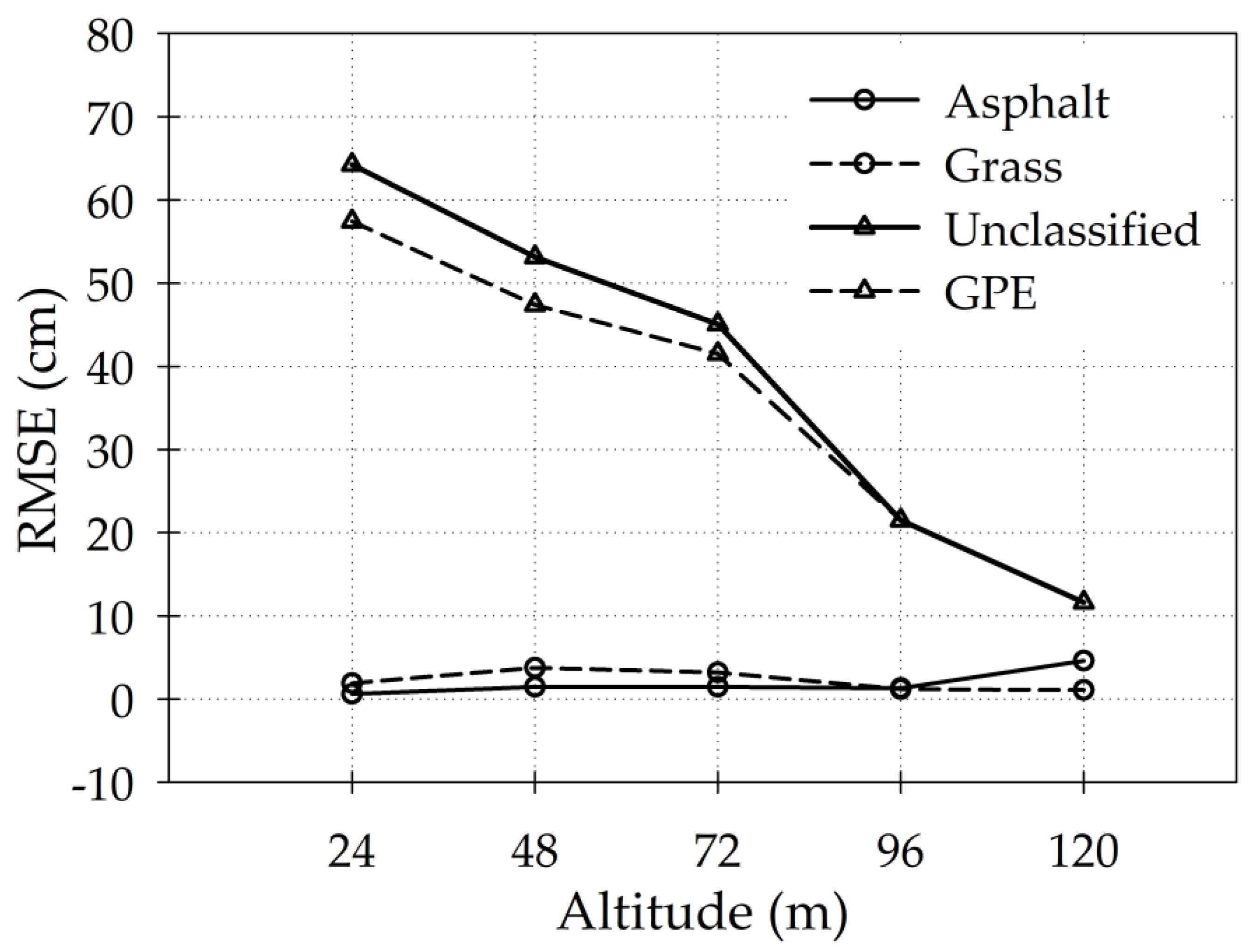
Figure 8 displays RMSE values generated using all control and marsh site data points collected throughout the duration of this study. Overall, J. roemerianus marsh sites exhibited a negative linear trend (adj. r2 = 0.93) in RMSE with increases in altitude. Values for the control site remained constant for all altitudes with minor discrepancies between asphalt and grass ground surface types. RMSE values for grass surfaces were slightly greater (≤2 cm) than those for asphalt at the 3 lowest altitudes. For 120 m AGL, the RMSE value for asphalt climbed to ~4.5 cm.

3.2. LiDAR Return Density and Distribution

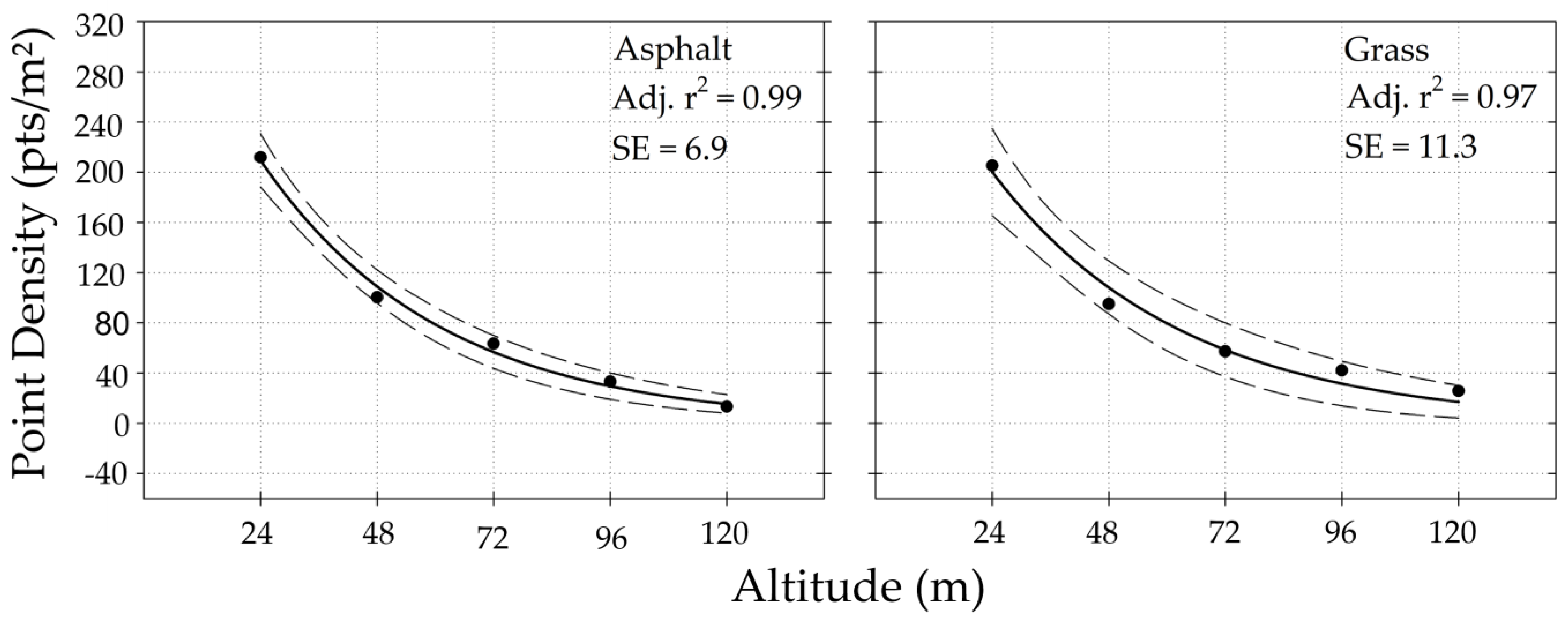
Areal density of LiDAR returns among all datasets decreased exponentially with increase in altitude AGL (Figure 9 and Figure 10). For the control site, adjusted coefficient of determination (r2) values were ≥0.97 for both paved and grass surface types (Figure 9). For altitudes greater than 48 m at marsh sites, most datasets consisted primarily of 0° scan angle returns with few off-nadir returns. Adjusted r2 values for marsh datasets were ≥0.98. For the control and marsh sites, some buffers were excluded from analysis due to an absence of LiDAR returns (Table 2).

3.3. Impacts of Surface Characteristics

The linear mixed-effects model indicated that the fixed effects (Inundation Depth, Erect Canopy Height, Flattened Canopy Height, and Altitude) explained 57% of the variability in LiDAR height difference (marginal r2 = 0.57). Although there were differences in vertical height difference among sites, these site differences only explained 6% of the variability in the data (ICC = 0.06), with the inclusion of the random effects improving the r-squared value of the model by around 2% (conditional r2 = 0.59) (Table 3 and Table 4).
Independent of the variation seen among sites, altitude (m) had a significant negative effect on the vertical difference in LiDAR returns compared with GNSS reference measurements (p < 0.05, beta = −0.20 cm) (Table 5). This indicates that every 10 m increase in flight altitude was associated with an accuracy improvement of 2 cm. Additionally, inundation depth (cm) and erect canopy height (cm) significantly affected vertical accuracy (p < 0.001), with erect canopy height demonstrating a positive effect on vertical difference (beta = 0.25 cm) and inundation depth demonstrating a negative effect (beta = −3.47 cm). The effect of the height of flattened sections of canopy had a relatively large positive effect on vertical difference (beta = 0.39 cm). However, this effect was not significant in the model (p = 0.019). This may be related to the distribution of the data values, which included many zero values where no flattened canopy was present but fewer observations with nonzero flattened canopy heights, with some flights only having a single measurement.

4. Discussion

The presence of dense, homogenous vegetation canopies has hindered aerial LiDAR mapping and monitoring efforts of coastal marshes. Remotely sensed ground height estimates are often overestimated and resulting digital models of marsh ground surfaces are not accurately depicted. Although this discrepancy has been investigated for airplane-mounted LiDAR systems, the efficacy of UAS-LiDAR for mapping and monitoring of these environments has only recently been explored by a limited number of studies [15,30]. The influence of altitude on ground height estimates in coastal marshes has been briefly discussed or explored, but an in-depth analysis of this influence has not yet been reported. The study presented here used precise topographic measurement samples and UAS-LiDAR data collected at five different altitudes along a survey transect to characterize the influence of altitude and site surface characteristics on LiDAR ground height estimates in five J. roemerianus-dominated coastal marsh settings across the Mississippi Gulf Coast. A control site was surveyed using the same methods throughout the duration of this study for comparison. Furthermore, a novel ground classification method was used prior to analysis and compared to unclassified LiDAR point clouds to assess the influence of noise from vegetation canopy returns on ground estimation. The results indicated a strong influence of altitude on RMSE values within J. roemerianus marshes as compared to the control site. Although higher flight altitudes reduced error values, point density values decreased exponentially, making these higher accuracy datasets less useful for practical applications. Finally, the GPE classification method improved RMSE values from unclassified data but was ineffective at flight altitudes of 96 m and 120 m. Overall, the results indicate that the influence of marsh surface characteristics on LiDAR ground height estimates cannot be overlooked in data acquisition.

4.1. Influence of Altitude, Surface Characteristics, and Sensor Design

The inclusion of a control site for comparison with the five marsh sites was essential for characterizing the effect of data collection altitude on LiDAR ground height estimates. Throughout the duration of the study, RMSE values for observations of the control site were ≤5 cm for all altitudes with two exceptions of higher values (Table 2). These lower RMSE values in addition to the MAE values for the control targets at each site indicate that the sensor was operating correctly and consistently for all observations during the data collection period, and that altitude had little influence on ground/target estimates in a controlled setting. Contrarily, altitude had a strong influence on RMSE values of the five marsh sites. RMSE decreased with increases in altitude, with classified values ranging from 57 to 12 cm at the lowest and highest altitudes, respectively (Figure 8). However, an important consideration when interpreting these results is the coupled relationship between point density and distribution and altitude. For the two lowest altitudes, 24 m and 48 m, point density values were consistent between all sites, including the control site (Figure 9 and Figure 10). For altitudes exceeding 48 m, the average point densities were 37 pts/m2 and 11 pts/m2 for control and marsh sites, respectively, indicating a 70% decrease (Figure 9 and Figure 10). Moreover, LiDAR point density was not homogenous along the transects for all altitudes. Instead, there was a steep decline in the percentage of buffers containing points for the two highest altitudes, 96 m and 120 m (Table 4). Thus, increases in altitude may reduce RMSE values for marsh sites, but the usability of the data is limited due to the low density and sparse distribution of returns.
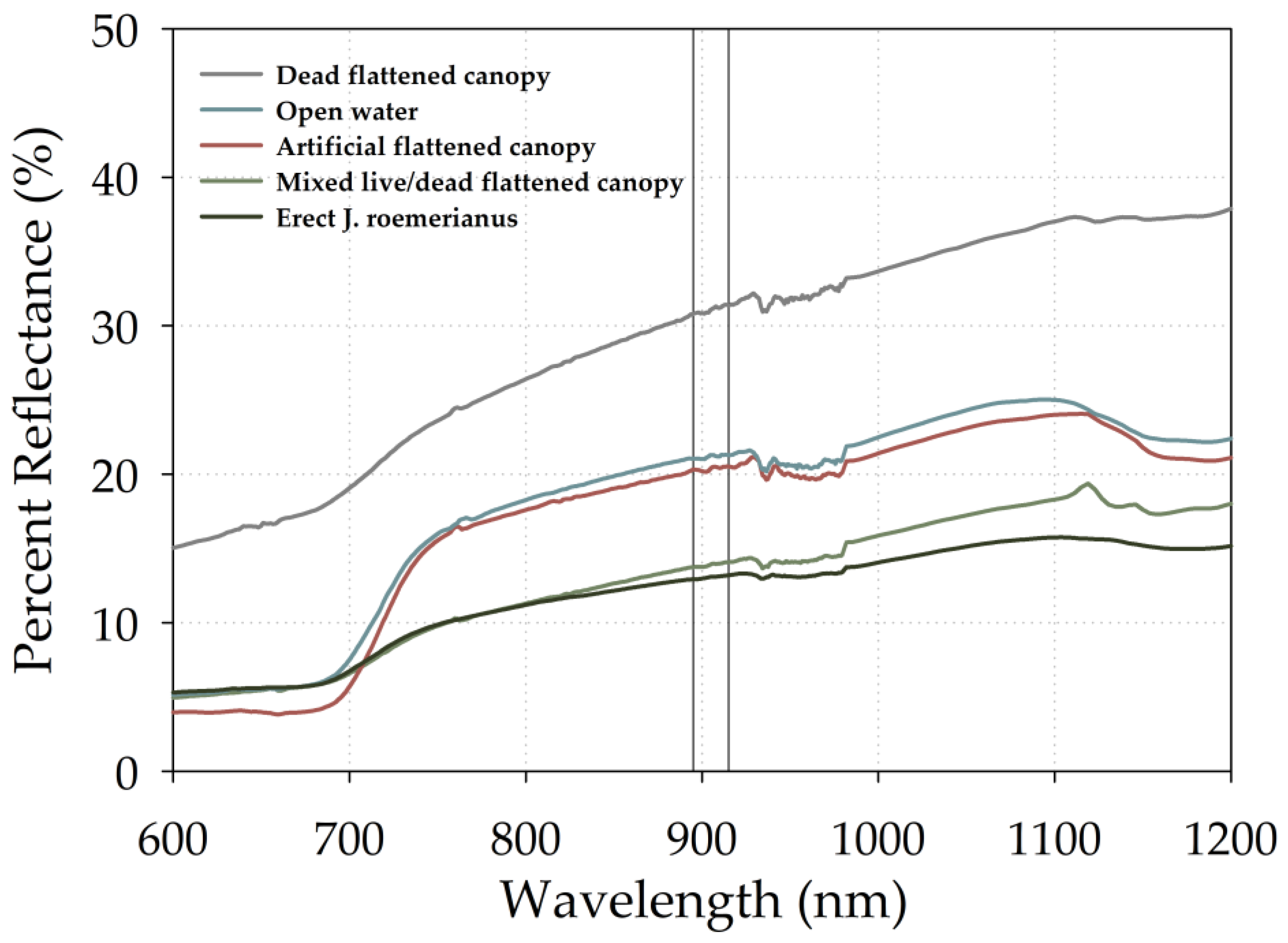
Vegetation characteristics such as species, canopy height and orientation, stem density, canopy cover, and spectral properties have been documented as being important contributing factors to error in LiDAR ground height estimates in marshes and other environments [22,29,30,48,49]. Although the current study focused only on one species, J. roemerianus, erect and flattened canopy height values for this species had notable influences on LiDAR ground height estimates (Table 5). Unsurprisingly, increased erect canopy height values were related to higher LiDAR ground height estimates, resulting in decreased accuracy (Table 5). However, the small but significant interaction between erect canopy height and altitude (beta = −0.002, p = < 0.001) demonstrated that as scanning altitude increased, canopy height had a weaker negative effect on accuracy. With an increased scanning altitude, the laser pulse is dispersed within the area of a larger laser footprint. Thus, only the most dense, lower portions of the erect canopy could be recorded by the system rather than the narrow, needle-like leaf tips of J. roemerianus. Hopkinson (2007) [48] demonstrated this concept previously in a wooded environment. Boucher et al. (2023) more recently investigated this relationship on grass, shrub, and tree canopies of a South African savanna [29]. Their findings corroborate this relationship and further emphasized the relevance of vegetation structure and composition [29]. The present study investigated the influences of vegetation structure by including both erect and flattened canopy height values into the linear mixed-effects model. Although flattened canopy height values were not significant as a main effect in this model, it appears that for datasets flown at altitudes ≥ 72 m, areas of flattened canopy and near-ground surfaces were among the few surfaces reflective enough to register a return and were thus highly visible in the point clouds. The needle-like growth form of J. roemerianus provides a challenging incidence angle for nadir aerial scanning. Accordingly, with increasing altitude, the likelihood of backscattering from erect leaves back to the sensor decreases. However, for flattened or dead canopy portions, incidence angle is improved, providing a surface for backscatter in the appropriate direction. Additionally, flattened canopy areas tended to have a higher proportion of dead leaves, likely contributing to higher reflectance at the wavelength of interest since dehydrated plant matter reflects more strongly in the near infrared [50,51]. These findings are supported by ancillary spectral data collected by the authors at the Wolf River survey site using a Spectra Vista HR-1024 spectroradiometer (Figure 11).
While near-infrared light is strongly absorbed by water, it can be scattered off water surfaces when the angle of incidence is low with respect to the normal [19,40,52]. Data collection efforts were all conducted within a few hours of the recorded low tide to minimize the effects of inundation. Regardless, all transects exhibited varying amounts of inundation, ranging from 0 to 33 cm. Greater water depths had a considerable positive influence on accuracy (Table 5). This could be attributable to the increased likelihood of scattering off water surfaces when the depth of inundation was greater. However, the interaction effect between altitude and water depth indicates this relationship is complicated (Table 5). As altitude increased, the effect of water depth on accuracy was less positive. This could be due to the decreased number of canopy returns at high altitudes, or that inundation depth was positively correlated with another unmeasured variable which impacted LiDAR return height. One potential variable could be vegetation density, which could theoretically have either a negative or positive relationship with inundation depth. While we did not measure vegetation density in a standardized way, we noted 37 sampling points which had particularly sparse or open canopy coverage. Of these 37, only 17 were associated with deeper-than-average inundation, indicating no relationship between open canopy and inundation depth. This further supports our hypothesis that inundation depth itself, over the range of values found in this study (0–33 cm), positively influences LiDAR accuracy due to interactions between the water and LiDAR pulses at varying altitudes. Other vegetation-related variables such as erect canopy height and flattened canopy height interacted with and modulated this effect of inundation depth (Table 5).
The relative influences of altitude and marsh surface characteristics on ground height estimates are affected by LiDAR sensor design. Discrete return LiDAR systems, such as the sensor used in this study, are often incapable of discerning multiple discrete returns less than 2 m apart [22,23,24,25,48]. This phenomenon occurs when the time between two subsequent returns from the same laser pulse is too short for the system to detect [22]. Therefore, when remotely sensing homogenous, dense, vegetative cover that is under 2 m in canopy height, subsequent returns from the underlying ground will not be recorded. Accordingly, the marsh ground or water surface was not detectable until scanning altitudes reached ≥72 m; the altitudes at which canopy returns were less abundant due to the reduced reflectivity of J. roemerianus. Spectral differences in vegetative cover would likely influence this relationship greatly. Therefore, other vegetation species and growth forms would likely have a unique interaction with similar sensors and should be considered during data collection planning, implementation, and result interpretation. An additional consideration is the LiDAR footprint. The sensor used for this study produced horizontal and vertical beam divergences of 0.08° and 0.8°, respectively [53]. Accordingly, the sensor produced an elongated, bar-shaped footprint that extended to over 1.5 m in length at a scanning altitude of 120 m. Uncertainty in ground height estimates may be added with enlarged footprint sizes. Previous studies have demonstrated this when investigating variable ground surface such as ground conditions with a sloped gradient [54,55] or those with a reflective object at the edge of the footprint area [56]. To the knowledge of the authors, this effect has not been demonstrated previously in heavily vegetated, coastal marsh environments, but is expected to influence LiDAR ground heights. Therefore, future investigations using sensors with similar beam divergence values should account for or quantify this effect.

4.2. GPE Classification Method

The GPE classification method improved RMSE from unclassified data, but was not effective for altitudes greater than 72 m. In these sparser datasets, marsh LiDAR return height ranges were equal to or less than those at the control site, resulting in no ground filtering being applied. Thus, the GPE classification approach can be considered useful for data collection efforts flown at lower altitudes, or when data density and return height ranges are greater, but the effectiveness of this method is reduced with increasing flight altitude. This finding further emphasizes the importance of data collection parameters on ground height estimates.
Comparisons between the GPE method and commonly used ground classification methods used in other studies are difficult due to differences in data collection parameters, sensor type, vegetation characteristics, and the proprietary nature of some methods. However, a similar, commonly used classification method is the minimum bin-gridding method [17,20,25,34,40]. This approach is often used for raster generation in vegetated environments. In this method, the user specifies the resolution of the output grid cells and the lowest point from within each grid cell determines the output grid cell height. The appropriate grid cell resolution varies based on the vegetation species, canopy height, and ground coverage present. Schmid et al. (2011) demonstrated this in investigating this ground classification method for J. roemerianus- and Spartina alterniflora-dominated sites [25]. Similarly, low-elevation points representing creeks and large canopy gaps at our study sites were preferentially selected using the GPE method when a larger area was used as the filtering window. As such, both methods are influenced greatly by spatial resolution. An important distinction between the two methods is that the minimum bin-gridding method relies on a single point within each grid cell to determine the output ground surface, whereas the GPE method uses a percentage of the lowest points. Relying on a single point increases the likelihood that erroneous, low points may be selected due to under sampling in areas where the slope is great or a low-lying feature is present [25]. However, inclusion of non-ground points is much more likely with the GPE method.
Although the GPE ground classification method served to represent the marsh ground surface more accurately as compared to an unclassified approach, future applications of this method would benefit from addressing key limitations and important parameters identified herein. The GPE method required a long-term average of return height ranges at a control site to develop a ground classification percentage estimation appropriate to the LiDAR sensor. Therefore, this method is likely less replicable than other classification methods for many applications. Another consideration for future applications of this method is data quantity. Data collection efforts for this study consisted of data capture along a single flight line. A larger quantity of data could be collected with the use of multiple flight lines and flight line crosshatching. A greater amount of data would likely increase marsh height ranges and subsequently decrease the percentage of marsh data to be classified as ground. Future applications of this method should consider this influence of data quantity and density on ground classification outputs. Tightly coupled with data acquisition parameters are the relative influences of sensor type and vegetation presence on GPE classification outputs. This study investigated marsh ground height estimate accuracy using one LiDAR sensor and dominant vegetation species. Different sensors and vegetation cover would influence classification outputs.

4.3. Considerations and Takeaways

The relationships among altitude, surface characteristics, sensor design, and ground height estimates presented in this article demonstrate that there is no easy solution to entirely remove vertical error in airborne LiDAR datasets of coastal marshes without correction factors for these variables. However, mitigation of this error during data collection is possible. This study identified a complex relationship between altitude and point density in which datasets collected at higher altitudes had less vertical error in ground height estimates, but point densities were too low to be feasible for applications outside of research. An idealistic scenario in which a LiDAR sensor with a variable or higher Pulse Repetition Frequency (PRF) was used could potentially increase point density, making higher altitude datasets more useful for practical applications. Additionally, a LiDAR system with a high enough power output per outgoing pulse could also have this same effect. Although these changes could ideally make high-altitude surveys practical, other sensor characteristics (e.g., beam divergence) could impact this relationship.
Although marsh surface characteristics influence ground height estimates greatly, these variables are difficult to quantify prior to resource expenditure towards aerial and ground surveys. Future research should prioritize quantifying these variables remotely at a fine spatial scale. Furthermore, future research should investigate the contribution of inundation depth on ground height estimates in more detail.

5. Conclusions

The enhanced susceptibility of coastal marshes to subsidence and sea-level rise has made elevation modeling of these environments increasingly important. Dense, homogenous vegetation that is characteristic of these landscapes hinders aerial remote sensing of precise elevation, but applications of UAS-LiDAR technology for environmental research and terrain modeling have shown promise. An exploration of the applicability of these systems for ground height estimation within challenging marsh environments is necessary. Furthermore, a holistic understanding of the relative influences of data acquisition altitude and marsh surface characteristics on ground height estimates is needed. To facilitate this understanding, this study examined these relationships and quantified their various influences for five J. roemerianus-dominated sites existing within Mississippi’s Coastal Preserves. Additionally, a novel ground classification method was employed to characterize LiDAR ground returns.
Average RMSE values for low altitude (24–72 m) and high altitude (96–120 m) datasets were 49 cm and 17 cm, respectively, demonstrating the gradual increase in accuracy with increasing flight altitude. Although RMSE values were reduced appreciably when datasets were collected at high altitude, point sparsity of these datasets greatly limits practical applications of these data. Linear mixed-effects modeling reinforced the strong influence of altitude on ground height estimates as well as marsh surface characteristics such as Water Depth and Erect Canopy Height. Of the variable inputs to this model, Altitude, Water Depth, and Erect Canopy Height had the largest effect on accuracy. Although less impactful, interaction effects among these inputs demonstrated the complex relationships between LiDAR footprint size, vegetation structure, and water presence. Accordingly, consideration of these variables is important for data collection efforts. In documenting these effects, the findings presented in this study contribute to the limited body of research concerned with obtaining more accurate ground height estimates in vulnerable coastal marsh settings. By considering the relationships presented here, future environmental mapping and monitoring efforts may be better informed.

Author Contributions

Conceptualization, M.A., C.P.A., M.C.B.W., G.T.R. and G.A.C.; methodology, M.A., C.P.A., M.C.B.W., G.T.R. and G.A.C.; software, M.C.B.W. and G.T.R.; validation, M.A., C.P.A., M.C.B.W., G.T.R. and G.A.C.; formal analysis, M.A., C.P.A., M.C.B.W., G.T.R. and G.A.C.; investigation, M.A., C.P.A., M.C.B.W., G.T.R. and G.A.C.; resources, M.A., C.P.A., M.C.B.W., G.T.R. and G.A.C.; data curation, M.A.; writing—original draft, M.A., C.P.A., M.C.B.W. and G.A.C.; writing—review and editing, M.A., C.P.A., M.C.B.W., G.T.R. and G.A.C.; visualization, M.A., C.P.A., M.C.B.W., G.T.R. and G.A.C.; supervision, M.A.; project administration, M.A.; funding acquisition, M.A., C.P.A., M.C.B.W., G.T.R. and G.A.C. All authors have read and agreed to the published version of the manuscript.

Funding

This research was funded by the National Oceanic and Atmospheric Administration (NOAA) National Geodetic Survey (NGS), grant number NA18NOS4000198.

Data Availability Statement

The raw data supporting the conclusions of this article will be made available by the authors on request.

Acknowledgments

The authors would like to thank Robert Gruba who supported both UAS data collection and LiDAR processing workflows; Sydni Crain, Steven Ates, and Andrew Smith for data collection; and Chris Brown and Debra Armstead for facility and technical support.

Conflicts of Interest

The authors declare no conflicts of interest.

References

  1. Hu, K.; Chen, Q.; Wang, H. A Numerical Study of Vegetation Impact on Reducing Storm Surge by Wetlands in a Semi-Enclosed Estuary. Coast. Eng. 2015, 95, 66–76. [Google Scholar] [CrossRef]
  2. Zhang, X.; Lin, P.; Gong, Z.; Li, B.; Chen, X. Wave Attenuation by Spartina Alterniflora under Macro-Tidal and Storm Surge Conditions. Wetlands 2020, 40, 2151–2162. [Google Scholar] [CrossRef]
  3. Willemsen, P.W.J.M.; Borsje, B.W.; Vuik, V.; Bouma, T.J.; Hulscher, S.J.M.H. Field-Based Decadal Wave Attenuating Capacity of Combined Tidal Flats and Salt Marshes. Coast. Eng. 2020, 156, 103628. [Google Scholar] [CrossRef]
  4. Kulawardhana, R.W.; Feagin, R.A.; Popescu, S.C.; Boutton, T.W.; Yeager, K.M.; Bianchi, T.S. The Role of Elevation, Relative Sea-Level History and Vegetation Transition in Determining Carbon Distribution in Spartina Alterniflora Dominated Salt Marshes. Estuar. Coast. Shelf Sci. 2015, 154, 48–57. [Google Scholar] [CrossRef]
  5. Moseman-Valtierra, S.; Abdul-Aziz, O.I.; Tang, J.; Ishtiaq, K.S.; Morkeski, K.; Mora, J.; Quinn, R.K.; Martin, R.M.; Egan, K.; Brannon, E.Q.; et al. Carbon Dioxide Fluxes Reflect Plant Zonation and Belowground Biomass in a Coastal Marsh. Ecosphere 2016, 7, e01560. [Google Scholar] [CrossRef]
  6. Leonard, L.A.; Luther, M.E. Flow Hydrodynamics in Tidal Marsh Canopies. Limnol. Oceanogr. 1995, 40, 1474–1484. [Google Scholar] [CrossRef]
  7. Reed, D.J. Sea-Level Rise and Coastal Marsh Sustainability: Geological and Ecological Factors in the Mississippi Delta Plain. Geomorphology 2002, 48, 233–243. [Google Scholar] [CrossRef]
  8. Eleuterius, L.N.; Caldwell, J.D. Soil Characteristics of Spartina Alterniflora, Spartina Patens, Juncus Roemerianus, Scirpus Olneyi, and Distichlis Spicata Populations at One Locality in Mississippi. Gulf Res. Rep. 1985, 8, 27–33. [Google Scholar] [CrossRef]
  9. Anderson, C.P.; Carter, G.A.; Waldron, M.C.B. Precise Elevation Thresholds Associated with Salt Marsh–Upland Ecotones along the Mississippi Gulf Coast. Ann. Am. Assoc. Geogr. 2022, 112, 1850–1865. [Google Scholar] [CrossRef]
  10. Wallace, L.; Bellman, C.; Hally, B.; Hernandez, J.; Jones, S.; Hillman, S. Assessing the Ability of Image Based Point Clouds Captured from a UAV to Measure the Terrain in the Presence of Canopy Cover. Forests 2019, 10, 284. [Google Scholar] [CrossRef]
  11. Lovitt, J.; Rahman, M.M.; McDermid, G.J. Assessing the Value of UAV Photogrammetry for Characterizing Terrain in Complex Peatlands. Remote Sens. 2017, 9, 715. [Google Scholar] [CrossRef]
  12. Rogers, S.R.; Manning, I.; Livingstone, W. Comparing the Spatial Accuracy of Digital Surface Models from Four Unoccupied Aerial Systems: Photogrammetry versus Lidar. Remote Sens. 2020, 12, 2806. [Google Scholar] [CrossRef]
  13. Akturk, E.; Altunel, A.O. Accuracy Assessment of a Low-Cost UAV Derived Digital Elevation Model (DEM) in a Highly Broken and Vegetated Terrain. Measurement 2019, 136, 382–386. [Google Scholar] [CrossRef]
  14. Correll, M.D.; Elphick, C.S.; Hantson, W.; Cline, B.B.; Tymkiw, E.L.; Gregory Shriver, W.; Olsen, B.J. A Multi-Scale Comparison of Elevation Measurement Methods in Northeastern Tidal Marshes of the United States. Wetlands 2019, 39, 633–643. [Google Scholar] [CrossRef]
  15. Pinton, D.; Canestrelli, A.; Wilkinson, B.; Ifju, P.; Ortega, A. Estimating Ground Elevation and Vegetation Characteristics in Coastal Salt Marshes Using UAV-Based LiDAR and Digital Aerial Photogrammetry. Remote Sens. 2021, 13, 4506. [Google Scholar] [CrossRef]
  16. Baltsavias, E.P. A Comparison between Photogrammetry and Laser Scanning. ISPRS J. Photogramm. 1999, 54, 83–94. [Google Scholar] [CrossRef]
  17. Cooper, H.M.; Zhang, C.; Davis, S.E.; Troxler, T.G. Object-Based Correction of LiDAR DEMs Using RTK-GPS Data and Machine Learning Modeling in the Coastal Everglades. Environ. Model. Softw. 2019, 112, 179–191. [Google Scholar] [CrossRef]
  18. Muñoz, D.F.; Cissell, J.R.; Moftakhari, H. Adjusting Emergent Herbaceous Wetland Elevation with Object-Based Image Analysis, Random Forest and the 2016 NLCD. Remote Sens. 2019, 11, 2346. [Google Scholar] [CrossRef]
  19. Rogers, J.N.; Parrish, C.E.; Ward, L.G.; Burdick, D.M. Improving Salt Marsh Digital Elevation Model Accuracy with Full-Waveform Lidar and Nonparametric Predictive Modeling. Estuar. Coast. Shelf Sci. 2018, 202, 193–211. [Google Scholar] [CrossRef]
  20. Rogers, J.N.; Parrish, C.E.; Ward, L.G.; Burdick, D.M. Assessment of Elevation Uncertainty in Salt Marsh Environments Using Discrete-Return and Full-Waveform Lidar. J. Coast. Res. 2016, 76, 107–122. [Google Scholar] [CrossRef]
  21. Tiner, R.W. Field Guide to Coastal Wetland Plants of the Southeastern United States, Illustrated ed.; University of Massachusetts Press: Amherst, MA, USA, 1993. [Google Scholar]
  22. Hladik, C.; Alber, M. Accuracy Assessment and Correction of a LIDAR-Derived Salt Marsh Digital Elevation Model. Remote Sens. Environ. 2012, 121, 224–235. [Google Scholar] [CrossRef]
  23. Rosso, P.H.; Ustin, S.L.; Hastings, A. Use of Lidar to Study Changes Associated with Spartina Invasion in San Francisco Bay Marshes. Remote Sens. Environ. 2006, 100, 295–306. [Google Scholar] [CrossRef]
  24. Nayegandhi, A.; Brock, J.C.; Wright, W.; O’Connell, M.J. Evaluating A Small Footprint Waveform-Resolving Lidar Over Coastal Vegetation Communities. Photogramm. Eng. Remote Sens. 2006, 12, 1407–1417. [Google Scholar]
  25. Schmid, K.A.; Hadley, B.C.; Wijekoon, N. Vertical Accuracy and Use of Topographic LIDAR Data in Coastal Marshes. J. Coast. Res. 2011, 27, 116–132. [Google Scholar] [CrossRef]
  26. Resop, J.P.; Lehmann, L.; Cully Hession, W. Drone Laser Scanning for Modeling Riverscape Topography and Vegetation: Comparison with Traditional Aerial Lidar. Drones 2019, 3, 35. [Google Scholar] [CrossRef]
  27. Alsadik, B.; Remondino, F. Flight Planning for LiDAR-Based UAS Mapping Applications. ISPRS Int. J. Geoinf. 2020, 9, 378. [Google Scholar] [CrossRef]
  28. Yao, H.; Qin, R.; Chen, X. Unmanned Aerial Vehicle for Remote Sensing Applications—A Review. Remote Sens. 2019, 11, 1443. [Google Scholar] [CrossRef]
  29. Boucher, P.B.; Hockridge, E.G.; Singh, J.; Davies, A.B. Flying High: Sampling Savanna Vegetation with UAV-lidar. Methods Ecol. Evol. 2023, 14, 7. [Google Scholar] [CrossRef]
  30. Curcio, A.C.; Peralta, G.; Aranda, M.; Barbero, L. Evaluating the Performance of High Spatial Resolution UAV-Photogrammetry and UAV-LiDAR for Salt Marshes: The Cádiz Bay Study Case. Remote Sens. 2022, 14, 3582. [Google Scholar] [CrossRef]
  31. Montane, J.M.; Torres, R. Accuracy Assessment of Lidar Saltmarsh Topographic Data Using RTK GPS. Photogramm. Eng. Remote Sens. 2006, 72, 961–967. [Google Scholar] [CrossRef]
  32. Fernandez-Nunez, M.; Burningham, H.; Ojeda Zujar, J. Improving Accuracy of LiDAR-Derived Digital Terrain Models for Saltmarsh Management. J. Coast. Conserv. 2017, 21, 209–222. [Google Scholar] [CrossRef]
  33. Eleuterius, L.N. The Marshes of Mississippi. Castanea 1972, 37, 153–168. [Google Scholar]
  34. Medeiros, S.; Hagen, S.; Weishampel, J.; Angelo, J. Adjusting Lidar-Derived Digital Terrain Models in Coastal Marshes Based on Estimated Aboveground Biomass Density. Remote Sens. 2015, 7, 3507–3525. [Google Scholar] [CrossRef]
  35. Mississippi Department of Marine Resources (MDMR). Coastal Preserves. Available online: https://dmr.ms.gov/coastal-preserves-2/ (accessed on 9 August 2022).
  36. Microdrones. Putting Microdrones to Work for You. Available online: https://www.microdrones.com/en/integrated-systems/expert-drone-line/mdlidar3000/?gclid=EAIaIQobChMI3LyNjMrR8QIVxMDICh1RUQkREAAYASAAEgK-cvD_BwE (accessed on 6 July 2021).
  37. Davidson, L.; Mills, J.P.; Haynes, I.; Augarde, C.; Bryan, P.; Douglas, M. Airborne to uas lidar: An analysis of uas lidar ground control targets. ISPRS—Int. Arch. Photogramm. Remote Sens. Spat. Inf. Sci. 2019, XLII-2/W13, 255–262. [Google Scholar] [CrossRef]
  38. Gulf Coast Geospatial Center (GCGC). Gulf Coast Geospatial Center Real-Time Network. Available online: http://rtn.usm.edu/default.aspx (accessed on 21 September 2023).
  39. Applanix. POSPac UAV v8.6. Available online: https://www.applanix.com/products/pospac-uav.htm (accessed on 21 September 2023).
  40. MdInfinity Desktop v2020.5. Available online: https://www.microdrones.com/en/content/drone-lidar-data-processing-made-easy-mdinfinity/ (accessed on 21 September 2023).
  41. Wang, C.; Menenti, M.; Stoll, M.P.; Feola, A.; Belluco, E.; Marani, M. Separation of Ground and Low Vegetation Signtures in LiDAR Measurements of Salt-Marsh Environments. IEEE Trans. Geosci. Remote Sens. 2009, 47, 2014–2023. [Google Scholar] [CrossRef]
  42. Pricope, N.G.; Halls, J.N.; Mapes, K.L.; Baxley, J.B.; Wu, J.J. Quantitative Comparison of UAS-Borne LiDAR Systems for High-Resolution Forested Wetland Mapping. Sensors 2020, 20, 4453. [Google Scholar] [CrossRef] [PubMed]
  43. Buffington, K.J.; Dugger, B.D.; Thorne, K.M.; Takekawa, J.Y. Statistical Correction of Lidar-Derived Digital Elevation Models with Multispectral Airborne Imagery in Tidal Marshes. Remote Sens. Environ. 2016, 186, 616–625. [Google Scholar] [CrossRef]
  44. Rapidlasso. LASTools. Available online: https://lastools.github.io/ (accessed on 21 September 2023).
  45. Brown, V.A. An Introduction to Linear Mixed-Effects Modeling in R. Adv. Methods Pract. Psychol. Sci. 2021, 4, 2515245920960351. [Google Scholar] [CrossRef]
  46. Bates, D.; Mächler, M.; Bolker, B.M.; Walker, S.C. Fitting Linear Mixed-Effects Models Using Lme4. J. Stat. Softw. 2015, 67. [Google Scholar] [CrossRef]
  47. Luke, S.G. Evaluating Significance in Linear Mixed-Effects Models in R. Behav. Res. Methods 2017, 49, 1494–1502. [Google Scholar] [CrossRef]
  48. Kenward, M.G.; Roger, J.H. Small Sample Inference for Fixed Effects from Restricted Maximum Likelihood. Biometrics 1997, 53, 983–997. [Google Scholar] [CrossRef]
  49. Hopkinson, C. The Influence of Flying Altitude, Beam Divergence, and Pulse Repetition Frequency on Laser Pulse Return Intensity and Canopy Frequency Distribution. Can. J. Remote Sens. 2007, 33, 312–324. [Google Scholar] [CrossRef]
  50. Zhao, X.; Su, Y.; Hu, T.; Cao, M.; Liu, X.; Yang, Q.; Guan, H.; Liu, L.; Guo, Q. Analysis of UAV Lidar Information Loss and Its Influence on the Estimation Accuracy of Structural and Functional Traits in a Meadow Steppe. Ecol. Indic. 2022, 135, 108515. [Google Scholar] [CrossRef]
  51. Carter, G.A. Responses of Leaf Spectral Reflectance to Plant Stress. Am. J. Bot. 1993, 80, 239–243. [Google Scholar]
  52. Jenson, J.R. Remote Sensing of the Environment: An Earth Resource Perspective, 2nd ed.; Pearson Education, Inc.: Upper Saddle River, NJ, USA, 2006. [Google Scholar]
  53. Tamari, S.; Mory, J.; Guerrero-Meza, V. Testing a Near-Infrared Lidar Mounted with a Large Incidence Angle to Monitor the Water Level of Turbid Reservoirs. ISPRS J. Photogramm. Remote Sens. 2011, 66, 585–591. [Google Scholar] [CrossRef]
  54. SICK Sensor Intelligence. LD-MRS 3D LiDAR Sensors. Available online: https://cdn.sick.com/media/docs/3/03/803/operating_instructions_ld_mrs_3d_lidar_sensors_en_im0032803.pdf (accessed on 21 September 2023).
  55. Hofton, M.A.; Rocchio, L.E.; Blair, J.B.; Dubayah, R. Validation of Vegetation Canopy Lidar Sub-Canopy Topography Measurements for a Dense Tropical Forest. J. Geodyn. 2002, 34, 491–502. [Google Scholar] [CrossRef]
  56. Su, J.; Bork, E. Influence of Vegetation, Slope, and Lidar Sampling Angle on DEM Accuracy. Photogramm. Eng. Remote Sens. 2006, 72, 1265–1274. [Google Scholar] [CrossRef]
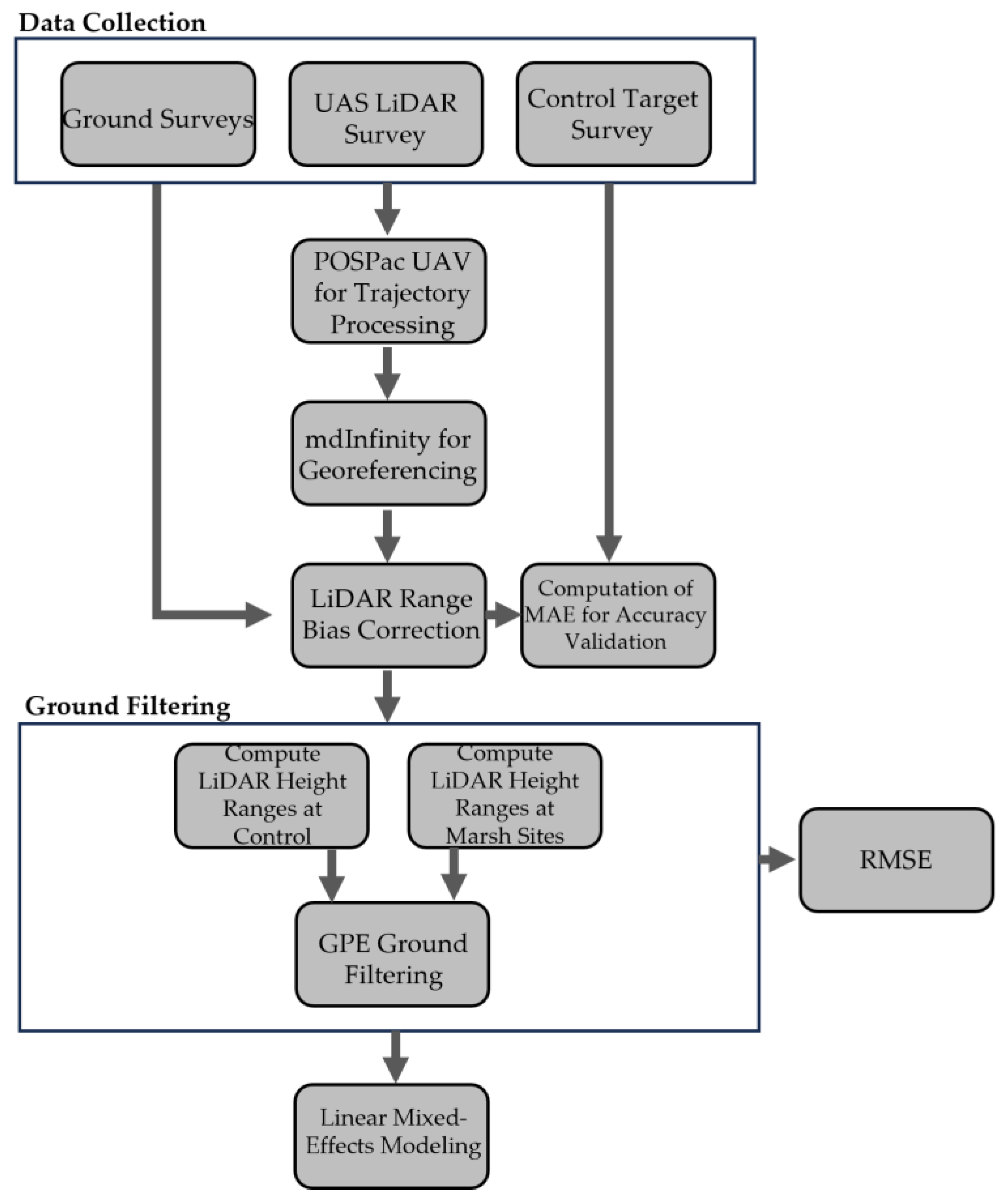
Figure 1. Flowchart outlining the major steps conducted in this study.
Remotesensing 16 00384 g001
Figure 2. Map of the study area showing the five study site locations and one control site location (black triangles) across Mississippi.
Remotesensing 16 00384 g002
Figure 3. Homogenous stands of J. roemerianus at the Wolf River Marsh Preserve.
Remotesensing 16 00384 g003
Figure 4. Control target set up in the Hancock County Marsh.
Remotesensing 16 00384 g004
Figure 5. MHD by altitude. Dashed lines indicate the 95% confidence intervals: y = 5.9 − 0.1 × altitude.
Remotesensing 16 00384 g005
Figure 6. RMSE by altitude for all occupations of the control site. Graphs are separated by ground surface type. Linear regression indicated the relationship between RMSE and altitude was not significant at alpha = 0.05 for the control site observations.
Remotesensing 16 00384 g006
Figure 7. RMSE by altitude for marsh site data. Graphs are separated by LiDAR ground classification type. Adjusted r2 values for GPE and Unclassified datasets were 0.67 and 0.75, respectively. The shaded area represents a 95% confidence interval.
Remotesensing 16 00384 g007
Figure 8. RMSE by altitude of the control site and marsh sites. Control site values are split by surface type asphalt (hollow circles with solid line) or grass (hollow circles with dashed line), and marsh values are split by classification type unclassified (hollow triangles with solid line) or GPE (hollow triangles with dashed line).
Remotesensing 16 00384 g008
Figure 9. Mean point density along the control transect. Each plotted value is the mean of 6 observations, and dashed lines represent the 95% confidence interval: y = a e b x .
Remotesensing 16 00384 g009
Figure 10. Mean point density along the marsh transects. Dashed lines display the 95% confidence interval: y = a e b x .
Remotesensing 16 00384 g010
Figure 11. Spectral reflectance curves of different marsh surface types obtained at the Wolf River survey site. Percent reflectance values were computed as an average of 5–10 measurements. Vertical reference lines represent the operating wavelengths of the LiDAR sensor. Over the operating wavelengths of the sensor, dead flattened canopy reflectance values were highest, followed by artificially flattened canopy and shallow (<10 cm) open water, with mixed live/dead flattened canopy and erect live canopy exhibiting the lowest reflectance values.
Remotesensing 16 00384 g011
Table 1. Computed correction factors for study altitudes. Values are rounded to cm precision.
Altitude (m)Correction Factors (cm)
24−3
48+0
72+3
96+6
120+9
Table 2. Mean percentage of buffers containing LiDAR returns for the control and marsh sites. The control site percentages were separated by ground surface type.
 Surface Type
Altitude (m)Grass (%)Asphalt (%)Marsh (%)
249910098
4810010098
7210010084
9610010034
1201005934
Table 3. Random effects (site) values.
Random Effects
σ2198.96
T00Site12.32
ICC0.06
N Site4
Observations815
Marginal r2/Conditional r20.568/0.593
Table 4. Conditional intercept terms added to the model based on the grouping variable (site).
GroupConditional Mean (cm)Conditional Standard Deviation (cm)
Graveline−3.4511.012
Hancock−2.0610.890
Pascagoula3.0101.042
Wolf2.5020.890
Table 5. Fixed effects of the linear mixed-effects model. Grey cells indicate significant variables (p-value = 0.05).
 Ground Height Difference (cm)
PredictorsEstimatesStd. Errorp-Value
(Intercept)29.358.01<0.001
Inundation depth (cm)−3.470.96<0.001
Erect canopy height (cm)0.250.05<0.001
Altitude (m)−0.200.100.048
Flattened canopy height (cm)0.390.300.189
Inundation depth × Flattened canopy height−0.030.010.003
Inundation depth × Erect canopy height0.030.01<0.001
Altitude × Flattened canopy height0.000.000.081
Inundation depth × Altitude0.010.000.013
Erect canopy height × Altitude−0.000.00<0.001
Erect canopy height × Flattened canopy height−0.000.000.399
Disclaimer/Publisher’s Note: The statements, opinions and data contained in all publications are solely those of the individual author(s) and contributor(s) and not of MDPI and/or the editor(s). MDPI and/or the editor(s) disclaim responsibility for any injury to people or property resulting from any ideas, methods, instructions or products referred to in the content.