Article

Global Polarimetric Synthetic Aperture Radar Image Segmentation with Data Augmentation and Hybrid Architecture Model

1
Key Laboratory of Microwave Imaging, Processing and Application Technology, Suzhou 215128, China
2
Suzhou Aerospace Information Research Institute, Suzhou 215128, China
3
Aerospace Information Research Institute, Chinese Academy of Sciences, Beijing 100049, China
4
School of Electronic, Electrical and Communication, Engineering, University of Chinese Academy of Sciences, Beijing 100049, China
5
National Key Laboratory of Microwave Imaging Technology, Beijing 100190, China
*
Author to whom correspondence should be addressed.
Remote Sens. 2024, 16(2), 380; https://doi.org/10.3390/rs16020380
Submission received: 15 November 2023 / Revised: 13 January 2024 / Accepted: 15 January 2024 / Published: 17 January 2024
(This article belongs to the Section AI Remote Sensing)

Abstract

:
Machine learning and deep neural networks have shown satisfactory performance in the supervised classification of Polarimetric Synthetic Aperture Radar (PolSAR) images. However, the PolSAR image classification task still faces some challenges. First, the current form of model input used for this task inevitably involves tedious preprocessing. In addition, issues such as insufficient labels and the design of the model also affect classification performance. To address these issues, this study proposes an augmentation method to better utilize the labeled data and improve the input format of the model, and an end-to-end PolSAR image global classification is implemented on our proposed hybrid network, PolSARMixer. Experimental results demonstrate that, compared to existing methods, our proposed method reduces the steps for the classification of PolSAR images, thus eliminating repetitive data preprocessing procedures and significantly improving classification performance.

1. Introduction

Polarimetric Synthetic Aperture Radar (PolSAR) is a radar technology that increases the polarization characteristic based on traditional Synthetic Aperture Radar (SAR). PolSAR facilitates the acquisition of polarization information from the target, thereby enabling more comprehensive and precise detection and imaging of the target. Additionally, PolSAR technology is an active remote sensing technology, unlike passive remote sensing technology (such as optical remote sensing), which is limited by weather and time [1]. Active remote sensing technology acquires data through the transmission of electromagnetic waves to the target and the reception of its reflected signals. Consequently, this method remains impervious to natural factors, such as variations in light intensity, cloud cover, haze, and sunlight. This attribute positions PolSAR technology with distinct advantages in promptly responding to emergencies and swiftly gathering target information. The application of PolSAR in ground target observation, such as land cover classification, is a very significant direction [2,3,4,5].
In the early stage, PolSAR image classification methods can be broadly categorized into two groups: those founded on scattering mechanisms [6,7,8] and those rooted in statistical approaches [9,10,11,12]. While both methods are characterized by simplicity, speed, and physical interpretability, their classification results tend to be coarse and imprecise. These approaches are primarily suited for the preliminary analysis of PolSAR data. With the emergence of deep neural networks, the data-driven self-learning representation mode of networks has attracted more and more attention. While the features acquired through deep networks may lack direct physical interpretability, their representational prowess significantly surpasses that of features manually extracted by human methods. Therefore, research has begun to introduce neural networks into PolSAR land cover classification. For example, Zhou et al. [13] used original polarimetric features from matrix T as input on the Flevoland I dataset and used a deep convolutional neural network for classification for the first time, and the classifier performance achieved the best performance at that time. In addition, because PolSAR data contain rich polarization information, such as scattering amplitude, polarization direction, and degree of polarization, this complex information may degrade the performance of unsupervised algorithms [14,15,16,17,18,19]. In contrast, supervised algorithms that utilize labeled data effectively learn the complex relationships of the data to improve performance [20,21,22,23,24,25,26,27]. Therefore, relying on extracting certain polarization features from the original scattering matrix as initial features and then letting the deep neural network learn higher-level and more complex features from the label data to improve the classification ability of the classifier has become a more efficient and popular method for PolSAR land cover classification.
At present, there are two primary strategies for PolSAR land cover supervised classification using deep neural networks, depending on the input of the model. The first strategy involves dividing the PolSAR image into small patches, with each patch representing a specific land cover class. Neural networks are then trained to recognize these small patches, thereby obtaining land cover classes across the entire image [28,29,30,31]. The second strategy, known as direct segmentation, entails feeding the PolSAR image into a neural network to directly segment the image, and then the trained model assigns each pixel to a specific land cover class [32,33,34]. Patch-based classification offers a high level of flexibility, and the model is easy to train, but it is sensitive to noise, and one patch represents a class, which will lead to the loss of spatial information because features spanning multiple patches cannot be accurately captured, resulting in classification errors. In addition, manually assigning a land cover label to each small patch can be a time-consuming and challenging task, especially for large and complex datasets. The direct segmentation strategy can quickly and comprehensively capture the spatial distribution information of land cover and has strong robustness and anti-noise ability. However, it has high requirements on the model, and due to computer performance limitations and limited label data, cut and merge operations (cutting image to 256 × 256 or lessx) are usually required on the original PolSAR images as input.
In general, due to the following issues, the performance of both patch-base and direct segmentation is still not ideal. (a) Redundant step. Both require redundant operation steps: patch construction or image cutting, which greatly increases the computational complexity. (b) Insufficient labeling data. PolSAR images typically have high resolution and cover a wide geographical area. Processing and annotating large-scale PolSAR data require a significant amount of time and computational resources. Due to the complexity of manual annotation, typically only some areas of the image contain labeled information. (c) Design of the model. In the domain of PolSAR image classification, models predominantly leverage Convolutional Neural Networks (CNNs) and Transformer architectures, each possessing distinctive advantages and limitations. CNNs excel at capturing local features, rendering them well-suited for conventional image tasks. However, when confronted with images featuring intricate boundaries, their restricted global contextual understanding may lead to suboptimal performance. In contrast, empowered by self-attention mechanisms, Transformer architectures demonstrate proficiency in handling global context, thereby enhancing their capability to recognize irregular boundaries. Nevertheless, they exhibit a diminished capacity for capturing local features, involve higher computational complexity, and necessitate a substantial amount of labeled data for effective training. Effectively leveraging the strengths of both architectures is a matter worthy of consideration.
In view of the challenges, this paper first presents a novel input for the model. This new format involves using the results obtained after applying the data augmentation methods proposed in this paper as input to the model. It aims to maximize the utilization of labeled data and overcome the shortcomings of previous strategies. Moreover, to accommodate this input format, a concise but superior model is proposed. Considering that Multiple Layers of Perceptron (MLP) have been proven to achieve long-range dependencies and significantly reduce computational complexity compared to Transformers [35], the model adopts a hybrid architecture that combines CNN and MLP to extract features at different levels. This hybrid architecture not only reduces computational complexity but also allows the observation of objects from a multiscale and long-range perspective. In addition, attention mechanisms have become a dominant paradigm in deep learning [36]. In this model, the use of cross-layer attention mechanisms aims to build global dependencies between features at different levels in PolSAR images.
The main contributions are summarized as follows:
(1)
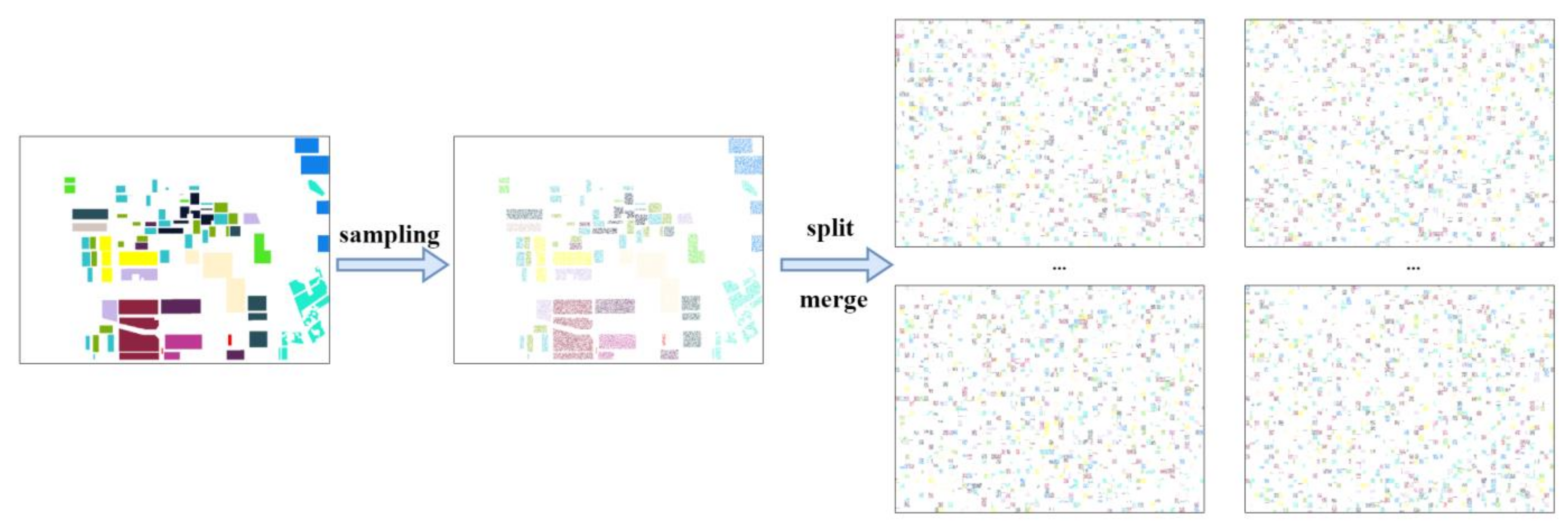
A data augmentation technique is introduced, aiming at significantly improving the utilization of labeled data while mitigating spatial information interference. Based on this data augmentation technique, we improved the input format without the need to construct patches or perform cut and merge operations on label data. This ensures the model can adapt to images of any size and swiftly conduct global inference.
(2)
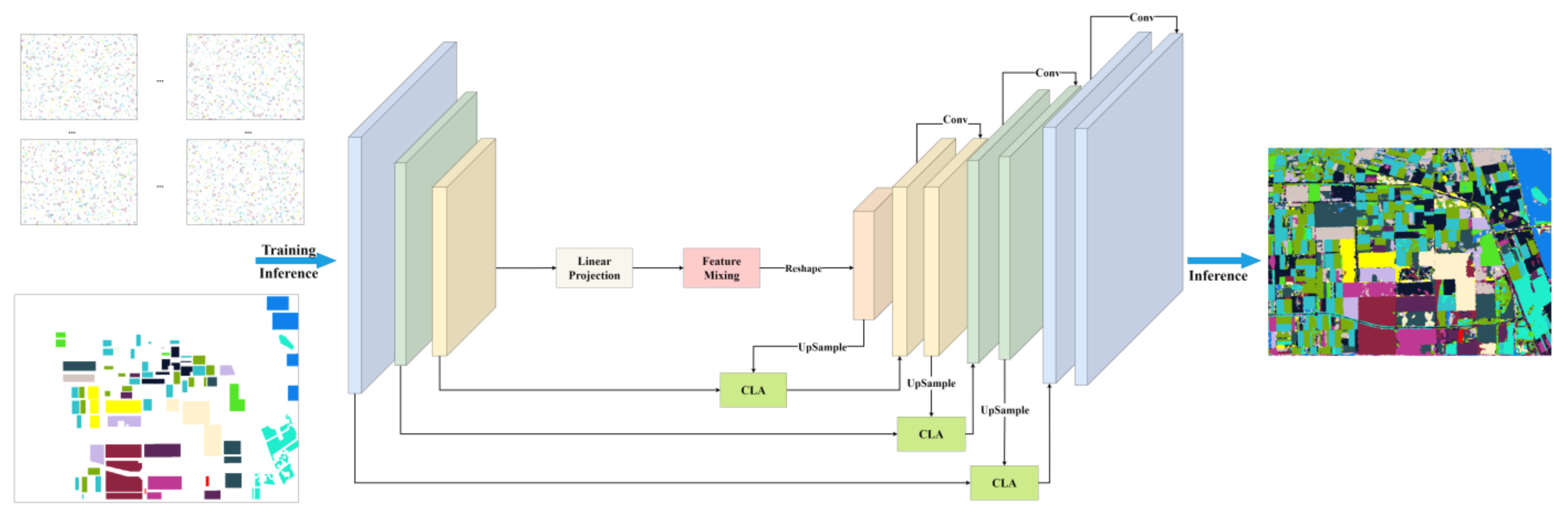
A hybrid architecture of CNN and MLP is proposed to classify PolSAR images. The architecture accepts arbitrary-size input images. Then, the output is the extracted feature at different levels.
(3)
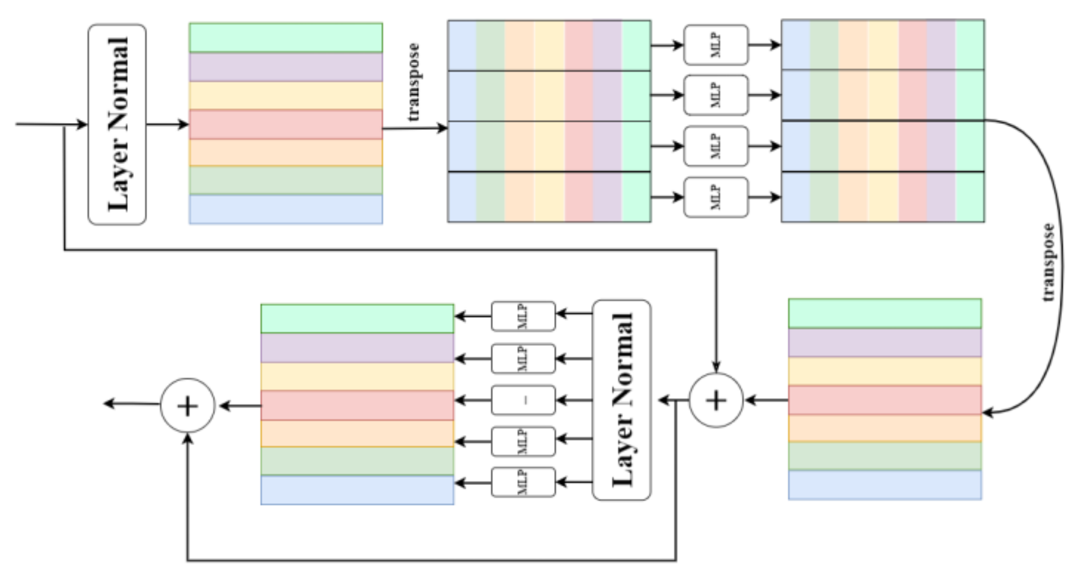
To further improve the performance, a cross-layer attention module is used to establish the relationship between different neural network layers, and the feature information is passed from the shallow layer to the deep layer. This information transfer helps capture dependencies over long distances, improving the model’s understanding of the data.
(4)
Three extensively recognized datasets are utilized for evaluating the efficacy of the proposed approach, and the experimental results unequivocally demonstrate its superior performance and classification accuracy when compared to contemporary other methods.
The rest of this paper is organized as follows: Section 2 focuses on the relevant attention mechanisms, the hybrid models, and the segmentation model. In Section 3, we elaborate on the details of the proposed methods. Section 4 provides a comprehensive analysis of comparative experimental results based on three extensively employed PolSAR images. Section 5 includes discussions on ablation experiments and analyzes the impact of hyperparameters in the proposed method. Lastly, in Section 6 and Section 7, we outline the potential directions for future research and draw conclusions.

2. Related Works

2.1. Segmentation Model

In the field of image segmentation, there are two key architectures. The first is based on the Fully Convolutional Network (FCN), which achieves downsampling and enlarges the receptive field through convolution operations. Deconvolution operations are then employed for upsampling to restore the original image size, thereby preserving the spatial information of the original input image and enabling pixel-level classification. The U-net, proposed by Ronneberger et al. [37], has been widely adopted due to its simple design and relatively small parameter count. However, its performance is relatively poor when dealing with larger images. Another important architecture adopts the Transformer structure, efficiently capturing global context through self-attention mechanisms and handling high-resolution images by independently processing image blocks. In this context, SETR, proposed by Zheng et al. [38], constructs an encoder solely using the Transformer without performing downsampling operations. It models the global context in each Transformer layer. While this encoder can be combined with a simple decoder to provide a powerful segmentation model, it requires higher computational complexity and has certain limitations in the interpretability of the self-attention mechanism.

2.2. Attention Mechanism

Attention Mechanism (AM), initially introduced for Machine Translation, has become a key concept in neural networks. It is widely used in various Artificial Intelligence applications, including Natural Language Processing (NLP) [39], Speech [40], and Computer Vision (CV) [41]. The Visual Attention Mechanism (VAE) has become popular in many mainstream CV tasks to focus on relevant regions within the image and capture structural long-range dependencies between parts of the image [42]. Among the different attention mechanisms, self-attention, multi-headed attention, and cross-attention are commonly used in CV tasks. Self-attention calculates the similarity between elements in an input sequence, updating each element’s representation based on the weights. Multi-head attention maps inputs to different subspaces, allowing the model to focus on diverse aspects simultaneously. Cross-attention addresses relationships between two sequences, with one sequence acting as a query vector and the other as a key-value vector, updating representations based on similarity weights.

2.3. Hybrid Model

Combining CNN and Transformer yields superior performance, with various approaches explored in recent studies. CMT, a visual network architecture, achieves enhanced performance by seamlessly integrating traditional convolution and Transformer [43]. It employs a multi-level Transformer with traditional convolution inserted between layers to hierarchically extract local and global image features. Conformer, a dual-network structure, merges CNN-based local features with Transformer-based global representations for improved representation learning [44]. Touvron et al. [45] proposed that DeiT, utilizing a CNN model as a teacher network, optimize Vit with hard distillation. This introduces the inductive bias feature of the CNN model into the Transformer, reducing data requirements, enhancing training speed, and achieving better performance. DETR, introduced by Carion et al. [46], adopts a concatenation method of CNN before the Transformer. The CNN network learns two-dimensional features, reshaping low-resolution feature maps for input into the Transformer, resulting in improved learning speed and overall model performance. ViT-FRCNN, proposed by Beal et al. [47], selects the Transformer before CNN. After ViT, Faster R-CNN is spliced sequentially as the target detection network, demonstrating the Transformer’s capability to retain spatial information for effective target detection.

3. Proposed Methods

3.1. PolSAR Data Augmentation Method

When labeled data are concentrated in a specific region, they can result in a substantial decline in the performance of the segmentation model when applied to segment the entire global image. This issue arises because, during training, the model tends to focus predominantly on the labeled area, potentially overlooking crucial information from other regions of the image. This phenomenon is frequently denoted as label skew or class imbalance. The model exhibits a learning bias as it lacks essential generalization capabilities, primarily stemming from its limited exposure to features from other regions. For instance, according to Equation (1), the spatial information of labeled data x i 0 , j 0 is still retained in the feature map obtained after a multi-layer neural network, demonstrating that the spatial information associated with labels in PolSAR images has the potential to disrupt the model’s capacity for global reasoning.
x i l , j l = f k l × k l f k l 1 × k l 1 f k 1 × k 1 x i 0 , j 0
To address the issues, a proven effective method involves distributing label data across various regions of the image. Through the random allocation of label data in different areas of the image, the model can mitigate the tendency to overly rely on information from specific regions. This approach enables the model to gain a more comprehensive understanding of the diverse features and structures within the image, thereby improving its generalization capabilities. This adaptation enhances the model’s ability to effectively handle challenges such as noise, occlusion, background changes, and more, ultimately bolstering its robustness.
Therefore, we randomly scrambled the label distribution without losing the original polarization characteristic information. The whole process can be expressed by the following formula:
X = f m e r g e f s p l i t f s a m p l e X ; θ ; σ ; τ
where X H × W × C is a PolSAR image and X is the new PolSAR image obtained. Three transformations: f s a m p l e , f s p l i t , f m e r g e can be formulated as:
u ¯ = f s a m p l e X ; ϑ = ϑ   ·   X
v ˜ = f s p l i t u ¯ ; σ h ; w = x 1 ; x 2 ; x n
X = f m e r g e v ˜ ; τ = τ v ˜ 11 τ v ˜ 1 w τ v ˜ h 1 τ v ˜ h w H × W
where ϑ is the sampling ratio, and ϑ % of points are used for each category in the labeled data; σ h ; w means the original image is divided into small blocks, x * h × w × C according to a fixed size h ; w , and τ shuffles the v ˜ and combines it into a new PolSAR image. For comparison, this paper maintains consistent shapes for both X and X .
Since this operation involves a direct split-merge process, it can be executed synchronously, allowing us to obtain multiple distinct new images simultaneously. The new images after data augmentation will be used as a training dataset. The entire procedure is illustrated in Figure 1.

3.2. Model

In this paper, we propose a model adapted to our input format, named PolSARMixer. The model’s architecture is depicted in Figure 2, primarily encompassing three key processes:
(1)
Shallow Feature Extraction: The whole PolSAR image is fed into the CNN network to extract preliminary features. The shallow features of PolSAR images at the i-th level are expressed as C o n v l o w i .
(2)
Deep Feature Extraction: To improve the perception of small targets, the final output C o n v l o w 3 of the shallow feature extraction module is forwarded to the Feature-Mixing (FM) blocks to obtain F M h i g h . Through the stacking of multiple Feature-Mixing layers, F M h i g h is highly integrated with both high-level abstract features and generalization features, aiding the model in better comprehending the content within images, enhancing segmentation performance for complex scenes and objects, reducing sensitivity to noise and variations, and delivering more semantically rich segmentation results.
(3)
Feature Fusion: High-level features provide abstract semantic information, while low-level features contain the details and basic structure of the image. Fusing these two types of information provides a more comprehensive understanding of the image and enhances the robustness of the model. To achieve enhanced utilization efficiency, F M h i g h is successively fused with the layers of C o n v l o w i through cross-layer attention (CLA) to obtain the multiscale high–low joint map.

3.2.1. Input of Model

The use of matrix T as a representation method for PolSAR images is widely recognized as an effective choice. This is because the elements within the matrix T offer physical interpretability to reflect the scattering mechanisms and scattering types of targets, thereby contributing to a deeper understanding of the content of the images. Furthermore, matrix T contains additional physical information, including the polarization characteristics and phase details of targets, which are crucial for enhancing the performance of deep learning models in classification tasks. Therefore, the input of the model is I n p u t H × W × 9 where H and W are the height and width of the original PolSAR image, and the vector of nine dimensions can be represented as:
v = T 11 , T 22 , T 33 , R e ( T 12 ) , I m ( T 12 ) , R e ( T 13 ) , I m ( T 13 ) , R e ( T 23 ) , I m ( T 23 )
where R e * and I m * represent the real and imaginary components of a complex value, respectively, and T * is the value of matrix T .

3.2.2. Feature Extractor

The shallow feature extractor is composed of three convolution layers with a convolution kernel of 3 × 3 and a stride of 2, which is used to scale feature maps to obtain a larger receptive field and extract features of different levels. The highest-level feature map C o n v l o w 3 H × W × C extracted from the CNN network is constructed into L S × C in Linear Projection module firstly, where S = H W p 2 is the number of non-overlapping image patches and p is the size of the patch. Then, L is linearly projected with the projection matrix M C × C to obtain L S × C . L is fed to the stacked Feature-Mixing blocks to enhance its perception of small targets. As shown in Figure 3, Feature-Mixing relies solely on MLP repeated in the spatial or feature channel domains, as well as basic matrix multiplication operations and data scale transformations, without the need for convolution or attention mechanisms. This design ensures a straightforward network structure and low computational complexity while maintaining global dependencies. It allows the model to capture the overall context and relationships, preserving contextual connections between objects and ensuring accurate segmentation of similar objects, thereby improving segmentation accuracy.
Furthermore, global dependencies are beneficial for the data augmentation techniques proposed in this paper. Through the shuffling and merging of label data, where targets span across multiple local regions, the introduction of global dependencies ensures that the model considers the relationships across these local regions, leading to improved segmentation of coherent objects.
The Feature-Mixer module is mainly composed of two sub-blocks. The first one is spatial mixing: it acts on rows of L , maps S 4 S S . The second one is channel mixing: it acts on a column of L , maps C 4 C C . Each sub-block contains two fully connected layers and a LayerNorm layer applied independently to ensure that the data of each patch is normalized in the feature dimensions. The Feature-Mixer block can be written as follows:
U = L + W 2 σ W 1 L a y e r N o r m L T T
V = U + W 4 σ W 3 L a y e r N o r m U
where σ is GELU, W 1 S × 4 S , W 2 4 S × S , W 3 C × 4 C and W 4 4 C × C are projection matrixes. The shape of the input and output of the Feature-Mixing block remains the same. The p is set as 2, and the output of stacking Feature-Mixer blocks is F M h i g h H 2 × W 2 × C   after reshaping.

3.2.3. Cross-Layer Attention

Cross-layer attention helps the model share information at different levels of abstraction, and its workflow is shown in Figure 4. It allows the model to transmit and exchange information about input data across different layers, thereby enhancing the overall model performance. Secondly, cross-layer attention aids in capturing long-range relationships and dependencies, thus improving the model’s representational capacity. Additionally, cross-layer attention enhances the model’s robustness. By sharing information at different levels, the model can better adapt to variations and noise in the input data, leading to improved performance in various scenarios.
First, 1 × 1 convolution is used to transform the features of C o n v l o w i into three identical feature maps: Q l o w i , K l o w i , and V l o w i of the same number of channels. In the same way, the F M h i g h used to obtain three identical feature maps: Q h i g h j , K h i g h j , V h i g h j .
Q l o w i , K l o w i , V l o w i = D c o n v C o n v l o w i , c = 3 c
Q h i g h j , K h i g h j , V h i g h j = D c o n v U p S a m p l e F M h i g h , c = 3 c
To obtain the cross-attention score for both, the transposes of K l o w i / K h i g h j and Q h i g h j / Q l o w i are multiplied and then normalized using the SoftMax function. The result is multiplied by V l o w i / V h i g h j to obtain the cross-attention maps C L A i / C L A j . Through matrix multiplication, the internal correlation of features is captured, and the long dependency between features is obtained, which can effectively model the context.
C L A i Q h i g h j , K l o w i , V l o w i = S o f t m a x Q h i g h j K l o w i T d V l o w i
C L A j Q l o w i , K h i g h j , V h i g h j = S o f t m a x Q l o w i , K h i g h j T d V h i g h j
The cross-information between low and high features is different, mutually independent, and complementary. The attention map of the high–low features cross-fusion in the j + 1 layer of the deep unit is expressed as follows:
F M h i g h = C L A i C L A j     ,           i + j = 3
Then, iterate layer by layer according to the above operation.

3.2.4. Loss Function

In the training process, after data augmentation, the target boundaries are extremely dispersed, and the uneven distribution of land cover categories, so the model is optimized by the Focal–Dice loss function to overcome these problems, which is written as:
L p , q = β 1 2 * p i q i p i + q i α p i 1 q i γ log q i
where p represents the target, q indicates the predicted probability, γ is the temperature coefficient, and α and β are weight factors, and for easy convergence of the model, we set α > β .

4. Experiments and Results

4.1. Dataset

To verify the effectiveness of our proposed method and model, we selected three PolSAR images for experiments, which are described below.
(1)
Flevoland I, AIRSAR, L-Band
Flevoland I is a widely used dataset for PolSAR classification, consisting of L-band data acquired at Flevoland, Netherlands, in 1989 by the Airborne Synthetic Aperture Radar (AIRSAR). The image scene size of the dataset is 750 × 1024 pixels. Of these, 157,296 pixels are labeled with 15 different terrain types. The categories marked include stem beans, rapeseed, bare soil, potatoes, beets, wheat 2, peas, wheat 3, lucerne, barley, wheat, grass, forest, water, and buildings. The pseudocolor image, ground truth, and legends of classes are shown in Figure 5.
(2)
Flevoland II, AIRSAR, L-Band
Flevoland II is another L-band quad-polarized dataset acquired by the AIRSAR in Flevoland, the Netherlands, in 1991. The dataset has an image scene size of 1024 × 1024 pixels, covering a total of 14 different terrain types and 122,928 annotated pixels. The categories included rapeseed, potato, barley, maize, lucerne, peas, fruit, wheat, beans, beets, grass, onions, and oats. The pseudocolor image, ground truth, and legends of classes are shown in Figure 6.
(3)
Oberpfaffenhofen, ESAR, L-Band
The Oberpfaffenhofen dataset is acquired from the L-band ESAR sensor that covers Oberpfaffenhofen, Germany. The image scene size of this dataset is 1300 × 1024 pixels, covering four different terrain types in total. The categories included Build-up Areas, Wood Land, and Open Areas. The pseudocolor image, ground truth, and legends of classes are shown in Figure 7.

4.2. Analysis Criteria of Performance

In this paper, Overall Accuracy (OA), Average Accuracy (AA), Mean Intersection over Union (mIoU), Mean Dice coefficient (mDice), and Kappa coefficient are the criteria to evaluate the model. OA is a metric used to evaluate the performance of a classification model, measuring the overall accuracy of the model on the entire dataset. AA takes the average accuracy of the model in each class and calculates the mean, providing a more comprehensive assessment of the model’s performance. The Kappa coefficient is a statistical metric used to measure consistency or agreement in classification tasks. The mIoU measures the average overlap between predicted and ground truth segmentation results, and the mDice measures the average similarity between predicted and ground truth segmentation results. These criteria are calculated as follows:
OA = T P N
AA = 1 C i = 1 C p i
K a p p a = P o P e 1 P e
mIOU = 1 C i = 1 C T P i T P i + F P i + F N i
mDice = 1 C i = 1 C 2 * T P i 2 * T P i + F P i + F N i
where T P is the number of samples that are correctly classified, N is the total number of samples, P o is observed agreement, P e is expected agreement, C is the total number of classes, and p i is the accuracy of the i-th class. T P i represents the number of samples that the model correctly predicted as class i , F P i represents the number of samples that the model incorrectly predicted as class i , and F N i represents the number of samples that the model incorrectly predicted as class i as some other class.

4.3. Parameters of Experiment

All the experiments are running on Ubuntu 18.04 LTS with a 48GB NVIDIA RTX8000 GPU. All these methods are implemented using the deep learning framework of Pytorch. We constructed three different input formats for comparison. In the patch-based (PB) construction method, the size of each patch is 8 × 8. In the direct segmentation (DS) construction method, we divide labeled areas into 32 × 32 sub-images. In the data augmentation (DA) formatted dataset, according to the method outlined in Section 3.1, 30% of points are selected to create training images, while another 30% of points are used to generate the validation images. All datasets are divided into training sets and validation sets in a 7:3 ratio. The configurations of different input formats are shown in Table 1.
We selected different classification models for different input formats to compare with our method. The compared models include SVM, CNN [48], U-net [37], and SETR [38]. The first two are models suitable for PB, and the latter two can take images of arbitrary sizes, so we tested their performance separately under conditions DS and DA. For all deep learning methods, we used Stochastic Gradient Descent (SGD) as the optimizer, with a weight decay coefficient set to 0.05, momentum set to 0.9, and an initial learning rate of 0.01. Additionally, PolyLR is employed as the learning rate scheduler, and the training epochs are fixed at 50.

4.4. Experiments Result

Table 2 presents the classification results, while Figure 8 depicts the visualized classification map of the Flevoland I dataset. The results from Table 2 indicate that the proposed model achieved an OA of 98.90%, outperforming SVM-PB (92.41%), CNN-PB (95.24%), U-Net-DS (94.68%), U-Net-DA (96.05%), SETR-DS (93.11%), and SETR-DA (98.29%). Comparative analysis across various criteria also highlights the superior performance of the PolSARMixer. Figure 8 provides a more detailed illustration of the issues with using PB-format data and DS-format data. In Figure 8c,d, noticeable noise points appear within the plots, and the boundary is unclear. Additionally, in Figure 8e,f, small details within the plots are lost, and there exists considerable transition disparity between segmented subplots. When utilizing U-Net with DA-format data, the transitions between subplots are smoother, the plot details are richer, and the evaluation criteria are higher. However, the global inference performance of SETA with DA-format data is not good. As can be seen from Figure 8h, its boundary range is not clear. The main reason is that the SETR model is not good at capturing local context when the label information of the dataset is limited. It is worth noting that our proposed PolSARMixer model demonstrates superior performance, offering clearer plot boundaries and fewer misclassifications.
Table 3 displays the evaluation results for the Flevoland II dataset. The data reveal that the proposed model outperforms other models in terms of AA, surpassing SVM-PB (91.17%), CNN-PB (96.98%), U-Net-DS (91.21%), SETR-DS (85.92%), U-Net-DA (96.61%), and SETR-DA (98.75%). Furthermore, the OA of PolSARMixer is notably higher than that of other methods by 1.82%, 2.71%, 1.35%, 2.84%, 0.39%, and 0.30%, respectively. Furthermore, the PolSARMixer achieves a mIoU of 98.14%, a mDice of 99.06%, and a Kappa coefficient of 0.9940. In Figure 9, class-wise land-cover classification maps for the Flevoland II region are depicted using various methods. It can be seen that PB-format data and DS-format data still have the problems of too many noise points and unclear boundaries. When U-Net is employed with DA-format data, as evident from Figure 9g, significant errors within large land parcels become noticeable. This is primarily due to its limited ability to capture long-range dependencies. From Figure 9i, it is evident that our model performs exceptionally well within both large and small land parcels. The parcels exhibit greater consistency, and the boundaries are notably clearer in the surrounding areas.
The class-wise land-cover classification map using various methods for the Oberpfaffenhofen dataset is shown in Figure 10. From Table 4, the results show that the proposed approach obtains the best classification performance and reaches 95.32% of OA, 93.85% of AA, 89.60% of mIoU, 94.46% of mDice, and 0.9176 of Kappa. It is obvious that the other methods have more misjudgment points in each category, but our proposed method only has a few misjudgment points in the Build-up category.

5. Analysis

5.1. Ablation Experiments

In this section, we conduct a comprehensive assessment of the individual modules within our proposed methodology and their impact on classification performance. Our results are succinctly summarized in Table 5. The data presented in Table 5 illustrate the substantial positive influence of both the Feature-Mixing and cross-layer attention modules on classification performance. The introduction of the Feature-Mixing module significantly improves the performance of different datasets. OA increased by 2.46%, 0.09%, and 1.23%; AA increased by 4.75%, 2.14%, and 0.99%; mIoU increased by 5.94%, 3.07%, and 2.24%; mDice increased by 3.94%, 1.67%, and 1.32%; and the Kappa coefficient increased by 2.69%, 0.10%, and 2.25%, respectively. This enhancement is primarily attributed to its capacity to extract high-level features by long-distance dependency, thereby enabling the extraction of features with strong generalization and the realization of a higher-dimensional observation scale. The cross-layer attention module results in an increase in OA values of 1.81%, 0.06%, and 1.35%; AA values of 1.81%, 1.94%, and 1.75%; mIoU values of 5.30%, 2.88%, and 2.50%; mDice values of 3.07%, 1.57%, and 1.48%; and Kappa coefficient values of 1.98%, 0.06%, and 2.51% across the three datasets. This module demonstrates effectiveness in capturing dependencies in spatial features across various layers, facilitating the efficient merging of information from different layers. Remarkably, when both modules are combined, the evaluation criteria reach the highest values for all datasets. This demonstrates the complementary and synergistic relationship between the two modules, which together can help with a significant improvement in classification performance.

5.2. Impact of Augmentation of Data

To verify the necessity of the data augmentation proposed in this paper, we further conducted experiments without data augmentation. For consistency, other processing remains unchanged. As illustrated in Figure 11, the model exhibits a deficiency in its global reasoning capabilities when data augmentation is not applied. Furthermore, a detailed analysis of Figure 11a,b reveals that the inherent spatial information contained in the labeled data significantly disrupts the model, leading to inaccurate classifications within non-labeled regions. Additionally, without data augmentation, the model lacks generalization capability. Even in scenarios with a substantial number of labels, such as Oberpfaffenhofen, as illustrated in Figure 11c, the model still fails to accurately delineate boundaries. The comparative experiments presented above underscore the efficacy of the proposed data augmentation method. This method effectively activates the model’s capacity for global inference, even when operating with a limited number of labels.

5.3. Impact of Shape of Blocks

In the proposed data augmentation method, the parameter h ; w represents the size of the block, and its size directly affects the performance of the model. Therefore, experimental analysis was performed to evaluate the impact of h ; w on classification performance, and the results are shown in Table 6. As visually depicted in Figure 12, it becomes apparent that distinct block shapes yield varying effects across different datasets. Notably, for the Flevoland I dataset, employing 8 ; 8 , as exemplified by the red mark in Figure 12a, incurs an increase in classification errors within larger blocks. This observation extends to the Flevoland II dataset as well. Conversely, when opting for a larger size, such as 32 ; 32 , as illustrated by the red mark in Figure 12c,f, the classification errors increase for small blocks. This is particularly noteworthy for the Flevoland II dataset, leading to a substantial drop in classification accuracy. For the Flevoland 1 and Flevoland II datasets, the deployment of 16 ; 16 attains optimal performance across various criteria. Conversely, for the Oberpfaffenhofen dataset, when h ; w is set to 32 ; 32 , the misclassification is minimized and the boundary determination is clearer, while settings of 8 ; 8 and 16 ; 16 exhibit poor performance, as shown in Figure 12g,h. In summary, the results emphasize the substantial effect of the parameter h ; w on classification performance. Therefore, the value of h ; w should be adjusted according to the size of the region, with annotations. In essence, with the enlargement of the scope of the annotation region, the parameter h ; w needs to be increased to achieve optimal global inference efficiency.

5.4. Impact of Sampling Ratio

To further reduce the proportion of labeled data while ensuring the model’s generalization performance, we employed proportional sampling of labeled data during the data augmentation process. Previous experimental results have demonstrated that our method already has excellent performance. In this section, we will delve deeper into the impact of different sampling ratios on classifier performance. Sampling rates for each class range from 10% to 70%, with intervals of 10%. Figure 13 illustrates how the OA, AA, mIoU, mDice, and Kappa coefficients of different datasets change as the training sample sampling ratio changes. All these criteria increase as the sampling proportion grows. It is particularly noteworthy that even at a sampling rate of 10%, our model still exhibits outstanding performance. Therefore, our proposed method remains highly effective in the case of less labeled data.

6. Discussion

Through the analysis of the experimental results, it becomes evident that our proposed PolSAR image land classification method excels. As shown in Table 7, our approach can achieve outstanding global inference results without the need for intricate operations such as constructing patches and cutes and merges, significantly simplifying the process. Furthermore, the hybrid model incorporating a cross-layer attention mechanism that we introduced exhibits similarly remarkable performance. It possesses exceptional capabilities for contextual reasoning and global dependency analysis, ensuring excellent generalization and robustness. However, we have also identified some limitations in the proposed data augmentation method. Firstly, when comparing performance across different datasets, especially in datasets like Flevoland II, we observed skewed angles in the labeled data, which may result in the loss of spatial information when directly splitting based on squares and cause the model to prefer learning without angles. To address this issue, we are considering splitting based on the skewed angles derived from the labels, with the aim of improving performance. Additionally, the adoption of fixed-sized blocks has proven to be inadequate in accommodating the actual distribution of land blocks. Therefore, considering the use of multiple block sizes for the split operation can assist the model in adapting to the real-world distribution of land blocks, thus enhancing its ability to recognize land block boundaries.

7. Conclusions

In this study, land classification based on the PolSAR image is studied as follows: (1) A data augmentation method, it constructs new PolSAR images by splitting and merging labeled data on PolSAR images as the input of the model and improves the global segmentation ability, generalization, and robustness of the model. (2) PolSARMixer, a hybrid CNN and MLP network comprising multi-layer feature extraction and low–high-level feature fusion modules based on cross-layer attention, is developed. (3) We tested our algorithm and performed experiments on the Flevoland I, Flevoland II, and Oberpfaffenhofen datasets, which proved its advantages in accurate land cover classification and reduced processing steps. In addition, the ablation experiments were carried out on the relevant hyperparameters of the proposed method, and the further improvement direction is discussed.

Author Contributions

Conceptualization, Z.W. (Zehua Wang) and Z.W. (Zezhong Wang); Methodology, Z.W. (Zehua Wang); Software, Z.W. (Zehua Wang) and Z.W. (Zezhong Wang); Validation, Z.W. (Zezhong Wang); Formal analysis, Z.W. (Zehua Wang) and Z.W. (Zezhong Wang); Investigation, Z.W. (Zehua Wang); Resources, X.Q. and Z.Z.; Writing—original draft, Z.W. (Zehua Wang); Writing—review & editing, Z.W. (Zehua Wang), X.Q. and Z.Z.; Visualization, Z.W. (Zehua Wang); Supervision, X.Q. and Z.Z.; Funding acquisition, Z.Z. All authors have read and agreed to the published version of the manuscript.

Funding

This research was funded by National Key R&D Program of China under Grant 2023YFB3904900.

Data Availability Statement

Data are contained within the article.

Conflicts of Interest

The authors declare no conflicts of interest.

References

  1. Parikh, H.; Patel, S.; Patel, V. Classification of SAR and PolSAR images using deep learning: A review. Int. J. Image Data Fusion 2020, 11, 1–32. [Google Scholar] [CrossRef]
  2. Sato, M.; Chen, S.W.; Satake, M. Polarimetric SAR Analysis of Tsunami Damage Following the March 11, 2011 East Japan Earthquake. Proc. IEEE 2012, 100, 2861–2875. [Google Scholar] [CrossRef]
  3. Chen, S.W.; Sato, M. Tsunami Damage Investigation of Built-Up Areas Using Multitemporal Spaceborne Full Polarimetric SAR Images. IEEE Trans. Geosci. Remote Sens. 2013, 51, 1985–1997. [Google Scholar] [CrossRef]
  4. Chen, S.W.; Wang, X.S.; Sato, M. Urban Damage Level Mapping Based on Scattering Mechanism Investigation Using Fully Polarimetric SAR Data for the 3.11 East Japan Earthquake. IEEE Trans. Geosci. Remote Sens. 2016, 54, 6919–6929. [Google Scholar] [CrossRef]
  5. Datcu, M.; Huang, Z.; Anghel, A.; Zhao, J.; Cacoveanu, R. Explainable, Physics-Aware, Trustworthy Artificial Intelligence: A paradigm shift for synthetic aperture radar. IEEE Geosci. Remote Sens. Mag. 2023, 11, 8–25. [Google Scholar] [CrossRef]
  6. Cloude, S.R.; Pottier, E. An entropy based classification scheme for land applications of polarimetric SAR. IEEE Trans. Geosci. Remote Sens. 1997, 35, 68–78. [Google Scholar] [CrossRef]
  7. Freeman, A.; Durden, S.L. A three-component scattering model for polarimetric SAR data. IEEE Trans. Geosci. Remote Sens. 1998, 36, 963–973. [Google Scholar] [CrossRef]
  8. Yamaguchi, Y.; Moriyama, T.; Ishido, M.; Yamada, H. Four-component scattering model for polarimetric SAR image decomposition. IEEE Trans. Geosci. Remote Sens. 2005, 43, 1699–1706. [Google Scholar] [CrossRef]
  9. Lee, J.S.; Grunes, M.R.; Ainsworth, T.L.; Du, L.J.; Schuler, D.L.; Cloude, S.R. Unsupervised classification using polarimetric decomposition and the complex Wishart classifier. IEEE Trans. Geosci. Remote Sens. 1999, 37, 2249–2258. [Google Scholar] [CrossRef]
  10. Lee, J.S.; Schuler, D.L.; Lang, R.H.; Ranson, K.J. K-distribution for multi-look processed polarimetric SAR imagery. In Proceedings of the International Geoscience and Remote Sensing Symposium on Surface and Atmospheric Remote Sensing—Technologies, Data Analysis and Interpretation (IGARSS 94), Pasadena, CA, USA, 8–12 August 1992; pp. 2179–2181. [Google Scholar]
  11. Doulgeris, A.P. An Automatic U-Distribution and Markov Random Field Segmentation Algorithm for PolSAR Images. IEEE Trans. Geosci. Remote Sens. 2015, 53, 1819–1827. [Google Scholar] [CrossRef]
  12. Doulgeris, A.P.; Anfinsen, S.N.; Eltoft, T. Automated Non-Gaussian Clustering of Polarimetric Synthetic Aperture Radar Images. IEEE Trans. Geosci. Remote Sens. 2011, 49, 3665–3676. [Google Scholar] [CrossRef]
  13. Zhou, Y.; Wang, H.P.; Xu, F.; Jin, Y.Q. Polarimetric SAR Image Classification Using Deep Convolutional Neural Networks. IEEE Geosci. Remote Sens. Lett. 2016, 13, 1935–1939. [Google Scholar] [CrossRef]
  14. Liu, F.; Jiao, L.C.; Hou, B.; Yang, S.Y. POL-SAR Image Classification Based on Wishart DBN and Local Spatial Information. IEEE Trans. Geosci. Remote Sens. 2016, 54, 3292–3308. [Google Scholar] [CrossRef]
  15. Xie, W.; Jiao, L.C.; Hou, B.; Ma, W.P.; Zhao, J.; Zhang, S.Y.; Liu, F. POLSAR Image Classification via Wishart-AE Model or Wishart-CAE Model. IEEE J. Sel. Top. Appl. Earth Obs. Remote Sens. 2017, 10, 3604–3615. [Google Scholar] [CrossRef]
  16. Wang, J.L.; Hou, B.; Jiao, L.C.; Wang, S. POL-SAR Image Classification Based on Modified Stacked Autoencoder Network and Data Distribution. IEEE Trans. Geosci. Remote Sens. 2020, 58, 1678–1695. [Google Scholar] [CrossRef]
  17. Li, Y.Y.; Xing, R.T.; Jiao, L.C.; Chen, Y.Q.; Chai, Y.T.; Marturi, N.; Shang, R.H. Semi-Supervised PolSAR Image Classification Based on Self-Training and Superpixels. Remote Sens. 2019, 11, 1933. [Google Scholar] [CrossRef]
  18. Bi, H.X.; Sun, J.; Xu, Z.B. A Graph-Based Semisupervised Deep Learning Model for PolSAR Image Classification. IEEE Trans. Geosci. Remote Sens. 2019, 57, 2116–2132. [Google Scholar] [CrossRef]
  19. Fukuda, S.; Katagiri, R.; Hirosawa, H. Unsupervised approach for polarimetric SAR image classification using support vector machines. In Proceedings of the IEEE International Geoscience and Remote Sensing Symposium (IGARSS 2002)/24th Canadian Symposium on Remote Sensing, Toronto, ON, Canada, 24–28 June 2002; pp. 2599–2601. [Google Scholar]
  20. Kong, J.A.; Swartz, A.A.; Yueh, H.A.; Novak, L.M.; Shin, R.T. Identification of terrain cover using the optimum polarimetric classifier. J. Electromagn. Waves Appl. 1988, 2, 171–194. [Google Scholar]
  21. He, C.; Li, S.; Liao, Z.X.; Liao, M.S. Texture Classification of PolSAR Data Based on Sparse Coding of Wavelet Polarization Textons. IEEE Trans. Geosci. Remote Sens. 2013, 51, 4576–4590. [Google Scholar] [CrossRef]
  22. Masjedi, A.; Zoej, M.J.V.; Maghsoudi, Y. Classification of Polarimetric SAR Images Based on Modeling Contextual Information and Using Texture Features. IEEE Trans. Geosci. Remote Sens. 2016, 54, 932–943. [Google Scholar] [CrossRef]
  23. Hong, D.F.; Yokoya, N.; Chanussot, J.; Zhu, X.X. CoSpace: Common Subspace Learning From Hyperspectral-Multispectral Correspondences. IEEE Trans. Geosci. Remote Sens. 2019, 57, 4349–4359. [Google Scholar] [CrossRef]
  24. Zhang, L.; Ma, W.P.; Zhang, D. Stacked Sparse Autoencoder in PolSAR Data Classification Using Local Spatial Information. IEEE Geosci. Remote Sens. Lett. 2016, 13, 1359–1363. [Google Scholar] [CrossRef]
  25. Jiao, L.C.; Liu, F. Wishart Deep Stacking Network for Fast POLSAR Image Classification. IEEE Trans. Image Process. 2016, 25, 3273–3286. [Google Scholar] [CrossRef] [PubMed]
  26. Chen, Y.Q.; Jiao, L.C.; Li, Y.Y.; Li, L.L.; Zhang, D.; Ren, B.; Marturi, N. A Novel Semicoupled Projective Dictionary Pair Learning Method for PolSAR Image Classification. IEEE Trans. Geosci. Remote Sens. 2019, 57, 2407–2418. [Google Scholar] [CrossRef]
  27. Fukuda, S.; Hirosawa, H. Polarimetric SAR image classification using support vector machines. IEICE Trans. Electron. 2001, E84C, 1939–1945. [Google Scholar]
  28. Jamali, A.; Roy, S.K.; Bhattacharya, A.; Ghamisi, P. Local Window Attention Transformer for Polarimetric SAR Image Classification. IEEE Geosci. Remote Sens. Lett. 2023, 20, 4004205. [Google Scholar] [CrossRef]
  29. Chen, S.-W.; Tao, C.-S. PolSAR image classification using polarimetric-feature-driven deep convolutional neural network. IEEE Geosci. Remote Sens. Lett. 2018, 15, 627–631. [Google Scholar] [CrossRef]
  30. Ni, J.; Xiang, D.; Lin, Z.; López-Martínez, C.; Hu, W.; Zhang, F. DNN-based PolSAR image classification on noisy labels. IEEE J. Sel. Top. Appl. Earth Obs. Remote Sens. 2022, 15, 3697–3713. [Google Scholar] [CrossRef]
  31. Li, L.; Ma, L.; Jiao, L.; Liu, F.; Sun, Q.; Zhao, J. Complex contourlet-CNN for polarimetric SAR image classification. Pattern Recognit. 2020, 100, 107110. [Google Scholar] [CrossRef]
  32. Fang, Z.; Zhang, G.; Dai, Q.; Xue, B.; Wang, P. Hybrid Attention-Based Encoder–Decoder Fully Convolutional Network for PolSAR Image Classification. Remote Sens. 2023, 15, 526. [Google Scholar] [CrossRef]
  33. Mohammadimanesh, F.; Salehi, B.; Mandianpari, M.; Gill, E.; Molinier, M. A new fully convolutional neural network for semantic segmentation of polarimetric SAR imagery in complex land cover ecosystem. ISPRS J. Photogramm. Remote Sens. 2019, 151, 223–236. [Google Scholar] [CrossRef]
  34. Zhang, R.; Chen, J.; Feng, L.; Li, S.; Yang, W.; Guo, D. A Refined Pyramid Scene Parsing Network for Polarimetric SAR Image Semantic Segmentation in Agricultural Areas. IEEE Geosci. Remote Sens. Lett. 2022, 19, 4014805. [Google Scholar] [CrossRef]
  35. Tolstikhin, I.; Houlsby, N.; Kolesnikov, A.; Beyer, L.; Zhai, X.H.; Unterthiner, T.; Yung, J.; Steiner, A.; Keysers, D.; Uszkoreit, J.; et al. MLP-Mixer: An all-MLP Architecture for Vision. In Proceedings of the 35th Conference on Neural Information Processing Systems (NeurIPS), Online, 6–14 December 2021. [Google Scholar]
  36. Vaswani, A.; Shazeer, N.; Parmar, N.; Uszkoreit, J.; Jones, L.; Gomez, A.N.; Kaiser, L.; Polosukhin, I. Attention Is All You Need. In Proceedings of the 31st Annual Conference on Neural Information Processing Systems (NIPS), Long Beach, CA, USA, 4–9 December 2017. [Google Scholar]
  37. Ronneberger, O.; Fischer, P.; Brox, T. U-net: Convolutional networks for biomedical image segmentation. In Medical Image Computing and Computer-Assisted Intervention–MICCAI 2015: 18th International Conference, Munich, Germany, October 5–9, 2015, Proceedings, Part III; Springer: Cham, Switzerland, 2015; pp. 234–241. [Google Scholar]
  38. Zheng, S.X.; Lu, J.C.; Zhao, H.S.; Zhu, X.T.; Luo, Z.K.; Wang, Y.B.; Fu, Y.W.; Feng, J.F.; Xiang, T.; Torr, P.H.S.; et al. Rethinking Semantic Segmentation from a Sequence-to-Sequence Perspective with Transformers. In Proceedings of the IEEE/CVF Conference on Computer Vision and Pattern Recognition (CVPR), Nashville, TN, USA, 19–25 June 2021; pp. 6877–6886. [Google Scholar]
  39. Galassi, A.; Lippi, M.; Torroni, P. Attention in natural language processing. IEEE Trans. Neural Netw. Learn. Syst. 2020, 32, 4291–4308. [Google Scholar] [CrossRef]
  40. Cho, K.; Courville, A.; Bengio, Y. Describing multimedia content using attention-based encoder-decoder networks. IEEE Trans. Multimed. 2015, 17, 1875–1886. [Google Scholar] [CrossRef]
  41. Wang, F.; Tax, D. Survey on the attention based RNN model and its applications in computer vision. arXiv 2016, arXiv:1601.06823. [Google Scholar]
  42. Mnih, V.; Heess, N.; Graves, A. Recurrent models of visual attention. Adv. Neural Inf. Process. Syst. 2014, 27, 1–9. [Google Scholar]
  43. Guo, J.; Han, K.; Wu, H.; Tang, Y.; Chen, X.; Wang, Y.; Xu, C. Cmt: Convolutional neural networks meet vision transformers. In Proceedings of the IEEE/CVF Conference on Computer Vision and Pattern Recognition, New Orleans, LA, USA, 18–24 June 2022; pp. 12175–12185. [Google Scholar]
  44. Gulati, A.; Qin, J.; Chiu, C.-C.; Parmar, N.; Zhang, Y.; Yu, J.; Han, W.; Wang, S.; Zhang, Z.; Wu, Y. Conformer: Convolution-augmented transformer for speech recognition. arXiv 2020, arXiv:2005.08100. [Google Scholar]
  45. Touvron, H.; Cord, M.; Douze, M.; Massa, F.; Sablayrolles, A.; Jégou, H. Training data-efficient image transformers & distillation through attention. In Proceedings of the International Conference on Machine Learning, Virtual, 18–24 July 2021; pp. 10347–10357. [Google Scholar]
  46. Carion, N.; Massa, F.; Synnaeve, G.; Usunier, N.; Kirillov, A.; Zagoruyko, S. End-to-end object detection with transformers. In Proceedings of the European Conference on Computer Vision, Glasgow, UK, 23–28 August 2020; pp. 213–229. [Google Scholar]
  47. Beal, J.; Kim, E.; Tzeng, E.; Park, D.H.; Zhai, A.; Kislyuk, D. Toward transformer-based object detection. arXiv 2020, arXiv:2012.09958. [Google Scholar]
  48. He, K.M.; Zhang, X.Y.; Ren, S.Q.; Sun, J.; IEEE. Deep Residual Learning for Image Recognition. In Proceedings of the 2016 IEEE Conference on Computer Vision and Pattern Recognition (CVPR), Seattle, WA, USA, 27–30 June 2016; pp. 770–778. [Google Scholar]
Figure 1. Illustration of data augmentation.
Remotesensing 16 00380 g001
Figure 2. Architecture of the PolSARMixer.
Remotesensing 16 00380 g002
Figure 3. Flowchart of the Feature-Mixing.
Remotesensing 16 00380 g003
Figure 4. Architecture of the CLA.
Remotesensing 16 00380 g004
Figure 5. Flevoland I dataset: (a) pseudocolor image; (b) ground truth.
Remotesensing 16 00380 g005
Figure 6. Flevoland II dataset: (a) pseudocolor image; (b) ground truth.
Remotesensing 16 00380 g006
Figure 7. Oberpfaffenhofen dataset: (a) pseudocolor image; (b) ground truth.
Remotesensing 16 00380 g007
Figure 8. The class-wise land-cover classification map of the Flevoland I dataset: (a) pseudocolor image; (b) ground truth; (c) SVM-PB; (d) CNN-PB; (e) U-Net-DS; (f) SETR-DS; (g) U-Net-DA; (h) SETR-DA; (i) proposed method.
Remotesensing 16 00380 g008
Figure 9. The class-wise land-cover classification map of the Flevoland II dataset: (a) pseudocolor image; (b) ground truth; (c) SVM-PB; (d) CNN-PB; (e) U-Net-DS; (f) SETR-DS; (g) U-Net-DA; (h) SETR-DA; (i) proposed method.
Remotesensing 16 00380 g009
Figure 10. The class-wise land-cover classification map of the Oberpfaffenhofen dataset: (a) pseudocolor image; (b) ground truth; (c) SVM-PB; (d) CNN-PB; (e) U-Net-DS; (f) SETR-DS; (g) U-Net-DA; (h) SETR-DA; (i) proposed method.
Remotesensing 16 00380 g010
Figure 11. The class-wise land-cover classification map without data augmentation: (a) Flevoland I; (b) Flevoland II; (c) Oberpfaffenhofen.
Remotesensing 16 00380 g011
Figure 12. The class-wise land-cover classification map of different shapes of cropped blocks: 8 × 8: (a,d,g); 16 × 16: (b,e,h); 32 × 32: (c,f,i).
Remotesensing 16 00380 g012
Figure 13. Classification performance of different sampling ratios: (a) Flevoland I; (b) Flevoland II; (c) Oberpfaffenhofen.
Remotesensing 16 00380 g013
Table 1. Configurations of different input formats.
DatasetPBDSDA
SizeTraining RatioValidation RatioSizeTraining PlotsValidation PlotsSizeTraining PlotsValidation Plots
Flevoland I8 × 870%30%32 × 32880376750 × 10247030
Flevoland II8 × 870%30%32 × 3210814621024 × 10247030
Oberpfaffenhofen8 × 870%30%32 × 32256510991300 × 10247030
Table 2. Classification results of different methods in the Flevoland I dataset.
ClassSVM-
PB
CNN-
PB
U-Net-
DS
SETR-
DS
U-Net-
DA
SETR-
DA
Ours-
DA
Stem beans98.5299.0399.7999.6698.4497.1399.42
Peas96.6198.5799.0599.3797.8196.0299.07
Forest93.7199.5198.1298.6798.0697.3199.18
Lucerne95.7986.6799.1899.1295.5696.5298.71
Wheat 293.3092.3898.3297.9197.4997.7999.12
Beet98.2099.0599.7298.6496.3893.0599.06
Potato94.2897.6297.998.1597.9394.6399.41
Bare soil55.110097.9339.0567.7898.6298.51
Grass81.9697.1494.2880.3489.9394.3498.19
Rapeseed81.6686.6799.0574.0196.2097.2998.12
Barley95.1590.4898.08100.091.7297.2198.38
Wheat 180.8810085.5393.3893.8396.8198.01
Wheat 396.4999.5399.3999.9498.0297.5299.09
Water99.6980.1168.7891.0298.2898.0699.34
Building95.5999.5288.220.082.0793.9196.71
OA92.4195.2494.6893.1196.0598.2998.90
AA90.4695.0994.8984.6293.3098.1298.69
mIoU84.8491.0189.1078.9289.5296.4197.52
mDice90.7695.1793.3984.3894.2598.1798.74
Kappa0.91340.93570.94650.92090.95670.98260.9879
Table 3. Classification results of different methods in the Flevoland II dataset.
ClassSVM-
PB
CNN-
PB
U-Net-
DS
SETR-
DS
U-Net-
DA
SETR-
DA
Ours-
DA
Potato99.7099.5299.3999.4699.8699.1099.72
Fruit99.98100.099.0492.6396.9999.5899.49
Oats88.89100.097.6788.9495.0699.5497.52
Beet97.6294.2598.2899.4899.5097.9499.51
Barley99.5897.6199.6399.4199.7698.7399.68
Onions31.9390.4786.1367.4385.9297.6997.26
Wheat99.7696.6799.8599.9599.7698.6799.67
Beans94.0592.38100.0100.090.3393.5197.84
Peas99.9310099.7586.5797.4797.9498.97
Maize79.2198.101.570.0093.1095.9597.56
Flax98.5094.7699.9579.599.1798.9399.30
Rapeseed99.3199.5399.8099.999.8498.3899.73
Grass93.8897.7198.1594.8698.0397.7598.71
Lucerne93.9196.6797.7694.7097.7299.1298.71
OA97.6996.8098.1696.6799.1299.2199.51
AA91.1796.9891.2185.9296.6198.7598.83
mIoU86.6987.7882.7976.2794.8997.9698.14
mDice91.2390.3984.3580.2897.2998.9699.06
Kappa0.94380.96740.97800.96030.98960.99060.9940
Table 4. Classification results of different methods in the Oberpfaffenhofen dataset.
ClassSVM-
PB
CNN-
PB
U-Net-
DS
SETR-
DS
U-Net-
DA
SETR-
DA
Ours-
DA
Build-up 61.1758.3768.4784.6187.4278.1991.83
Wood Land80.2998.5598.5495.8891.5583.5391.59
Open Areas98.1187.9895.2698.7797.0571.7898.12
OA85.5281.8588.6594.4793.6178.6795.32
AA79.8681.6387.4293.0992.0177.8393.85
mIoU69.2268.8475.6488.1486.3964.1789.60
mDice80.9281.0485.8093.6292.5978.1194.46
Kappa0.78140.81260.80640.90480.88620.59760.9176
Table 5. Performance contribution of each module.
DatasetMethodOAAAmIoUmDiceKappa
Flevoland IBase Method
+ FM
+ CLA
+ FM + CLA
96.0593.3089.5294.250.9567
98.5198.0595.4698.190.9836
97.8697.0094.8297.320.9765
98.9098.6997.5298.740.9879
Flevoland IIBase Method
+ FM
+ CLA
+ FM + CLA
99.1296.6194.8997.290.9896
99.2198.7597.9698.960.9906
99.1898.5597.7798.860.9902
99.5198.8398.1499.060.9940
OberpfaffenhofenBase Method
+ FM
+ CLA
+ FM + CLA
93.6192.0186.3992.590.8862
94.8493.0088.6393.910.9087
94.9693.7688.8994.070.9113
95.3293.8589.6094.460.9176
Table 6. Performance of different shapes of block.
Dataset   h ; w OAAAmIoUmDiceKappa
Flevoland I8 × 896.8395.6792.3595.960.9652
16 × 1698.9098.6997.5298.740.9879
32 × 3298.2697.8796.3898.160.9702
Flevoland II8 × 893.8068.9862.8266.510.9265
16 × 1699.5198.8398.1499.060.9940
32 × 3296.8780.9676.2379.600.9630
Oberpfaffenhofen8 × 888.2585.9976.0186.110.7867
16 × 1695.3293.8589.6094.460.9176
32 × 3296.9996.3293.4496.580.9476
Table 7. Comparison of different inputs of the model.
PreprocessingPatch
Base
Direct
Segmentation
Data
Augmentation
Construct Patch××
Cut and Merge××
Global Inference××
Disclaimer/Publisher’s Note: The statements, opinions and data contained in all publications are solely those of the individual author(s) and contributor(s) and not of MDPI and/or the editor(s). MDPI and/or the editor(s) disclaim responsibility for any injury to people or property resulting from any ideas, methods, instructions or products referred to in the content.

