Abstract
The risk of oil spills in the Arctic is growing rapidly as anthropogenic activities increase due to climate-driven sea ice loss. Detecting and monitoring fuel spills in the marine environment is imperative for enacting an efficient response to mitigate the risk. Microwave radar systems can be used to address this issue; therefore, we examined the potential of C-band polarimetric radar for detecting diesel fuel in freezing seawater under windy environmental conditions. We present results from a mesocosm experiment, where we introduced diesel fuel to a seawater-filled cylindrical tub at the Sea-ice Environmental Research Facility (SERF), University of Manitoba. We characterized the temporal evolution of the diesel-contaminated seawater and sea ice by monitoring the normalized radar cross section (NRCS) and polarimetric parameters (i.e., copolarization ratio (Rco), cross-polarization ratio (Rxo), entropy (H), mean-alpha (α), conformity coefficient (μ), and copolarization correlation coefficient (ρco)) at 20° and 25° incidence angles. Three stages were identified, with notably different NRCS and polarimetric results, related to the thermophysical conditions. The transition from calm conditions to windy conditions was detected by the 25° incidence angle, whereas the transition from open water to sea ice was more apparent at 20°. The polarimetric analysis demonstrated that the conformity coefficient can have distinctive sensitivities to the presence of wind and sea ice at different incidence angles. The H versus α scatterplot showed that the range of distribution is dependent upon wind speed, incidence angle, and oil product. The findings of this study can be used to further improve the capability of existing and future C-band dual-polarization radar satellites or drone systems to detect and monitor potential diesel spills in the Arctic, particularly during the freeze-up season.
Keywords:
arctic; oil spill; diesel fuel; monitoring; radar backscatter; sea ice; polarimetry; C-band scatterometer 1. Introduction
Due to global warming and climate change, sea ice thickness and its extent have drastically decreased in recent years [1,2]. Sea ice affects weather patterns, ocean circulation, coastal communities, and ecosystems, so the changes bring new challenges for transportation and natural resource development [1]. The reduction of Arctic sea ice has increased the number of ships operating in this region to access natural resources (e.g., fuel resupply ships, and mining) [3]. These activities are associated with a high risk of oil spills and other chemical releases, which negatively impact local populations of animals, plants, and humans [4,5,6,7]. These factors can also threaten on an international scale due to the crucial biological, cultural, and economic influence of the polar region [8]. Owing to the tragic consequences of the Deepwater Horizon incident in the Gulf of Mexico, many countries, including Canada, advised extra attempts to address immediate solutions for future oil spill events, particularly in the Arctic [9]. The ability to respond effectively and efficiently has been identified by the Arctic Council as a critical priority [10]. Among major challenges are remoteness, short windows of open water and daylight, inadequate infrastructure (i.e., not enough equipment to sustain large groups), and communication. Therefore, remote detection and surveillance techniques are critical to confront effectively and respond to potential oil spills in the Arctic [11].
It is expected that shipping traffic in the late summer and early fall will continue to increase in response to the later freeze-up [12]. Fall freeze-up is a complex time of year in the marine environment, as ice can develop rapidly in various forms depending upon the prevalent meteorological conditions [13,14]. When sea ice forms during calm conditions, it begins as frazil ice that accumulates at the water’s surface. If an oil spill were to occur during this time, the oil would readily reach the surface of the water and would form a slurry of seawater, ice, and oil. As a separate scenario, if the sea ice grows under typical congelation growth, the ice provides a semipermeable physical barrier between the ocean and the atmosphere. This type of ice is called nilas; it is highly saline, flexible with wave motion, and can easily be mobilized by dynamic ocean conditions that cause overlapping (rafting), leads (openings in the sea ice), and ridging. If an oil spill occurs in this situation, an oil horizon will form beneath the sea ice and seek the surface, as the oil is less dense than seawater. In time, the oil would likely find its way to the surface through brine channels, pockets, and cracks in the ice. As a third scenario, we consider oil spills on the surface of the seawater. With subzero air temperatures, sea ice would begin to form beneath the oil spill. However, with wind and wave action, the oil could readily distribute laterally in the region, and some combination of dynamic forms of sea ice (e.g., pancake ice) would be seen. Detecting the location, extent, and trajectory of an oil spill is crucial for enacting an effective response plan. Current methods for detecting oil spills in the marine environment have detection times that are highly dependent upon the conditions. For example, in open water, an oil spill can be readily detected by a nearby observer or, if in a remote location, with an optical remote sensing satellite. When sea ice is present, the situation is significantly more complex. Various airborne and spaceborne remote sensing techniques can be used to increase the possibility of detecting the location and extent of an oil spill [15,16]. Spaceborne sensing operates over a large-scale area but is limited by long revisit cycles (e.g., an 8-day revisit cycle for both Landsat-5 and -7 and 2 days for MODIS), which fails to record significant changes between image acquisition intervals [15]. Conversely, airborne sensing methods can obtain high temporal resolution, although in a much smaller region. In addition, other remote sensing techniques (e.g., optical and radar sensors) have been evaluated likewise in spotting oil slicks on both airborne and spaceborne platforms [17]. Microwave radars are especially advantageous for transmitting and receiving signals in a range of frequencies independent of weather conditions and solar illumination which makes them a key component for polar science studies.
Nowadays, monitoring oil pollution in open water utilizes a combination of satellite- and aircraft-based single-polarization, active, microwave remote sensing systems (e.g., synthetic aperture radar (SAR) and scatterometers). In a recent study [18], single-polarization SAR was used to determine the impacts of oil on smoothing ocean capillary waves, which resulted in an area of decreased backscatter. The presence of sea ice complicates the behavior of spilled oil in which oil can migrate, partition, and accumulate below, within, and above the ice [19]. The freeze-up period can be a potential challenge for oil investigation where the formation of newly formed sea ice (NI), such as frazil, grease, and nilas, is prevalent. The challenge is that the oil-polluted NI and its surrounding clean ice can appear identical in SAR imagery [20]. NI is a solid heterogeneous mixture, which contains high volumes of liquid brine as well as air pockets (with a lesser fraction) in a pure ice background. During the formation of NI, the ice surface can be accompanied by the presence of moisture or frost flowers (depending on atmospheric conditions) due to its high salinity at its topmost layer.
To date, only a few studies have attempted to improve the contrast between NI and oil-contaminated sea ice using polarimetric SAR [20,21,22,23]. To improve the contrast ability in a polarimetric radar system, we can mathematically combine multipolarization signals to synthesize polarimetric parameters (e.g., copolarization ratio (Rco), cross-polarization ratio (Rxo), entropy (H), mean-alpha (α), conformity coefficient (μ), copolarization correlation coefficient (ρco), etc.). Previous studies were conducted using Rco, H, and to distinguish between oil-contaminated and oil-free ice scenes on SAR images [20,21,23,24]. Their results revealed that the Rco parameter had good separation potential, alongside H and , notably at lower incidence angles (<35°). A recent study [25] found that oil-contaminated ice can be discriminated from oil-free ice using 0.3-H and 18-degree mean-alpha. This finding was limited to crude oil, and our study is motivated to investigate this threshold in delineating diesel-contaminated ice. There are complementary studies that used alternative parameters to replace the H/α classification for polarimetric synthetic aperture radar (PolSAR) data. For instance, [26] demonstrated random similarity (with the similarity-based angle αs and entropy Hs, which measure the scattering mechanism and randomness of polarimetric scatterers, respectively), while [27] presented scattering diversity (or specific scattering predominance) and surface scattering fraction as H/α merited alternatives. Furthermore, several studies pointed out that ρco and μ parameters can be informative in distinguishing oil-contaminated and uncontaminated open water. In a recent study [25], conformity coefficient (μ) was also demonstrated as a complementary means to differentiate between crude oil-contaminated and uncontaminated ice.
The polarimetric microwave scattering response of sea ice is dependent upon the physical and thermodynamic state of the ice [28], thereby giving the potential to provide an additional metric for detecting or monitoring oil spills. The behaviors are mainly dependent on physical parameters such as sea-ice surface roughness and the heterogeneity level within the sea-ice medium. The Rco parameter is associated with changes in surface scattering, which increases with an increase in incidence angle [20,29]. Additionally, changing the volume scattering can potentially enhance the Rxo values through depolarization mechanisms (e.g., brine pocket rearrangements or oil movements within a homogenous ice volume) [24,30,31]. According to previous research (e.g., [25,32]), target decomposition (TD) theorems have been used to differentiate between surface and volume scattering behaviors.
However, true validations of theoretical studies are limited as the ability to conduct oil spill experiments remains heavily regulated in the Arctic regions [33]. Another limitation of these studies is the calibration accuracy of spaceborne and airborne systems, which can cause misinterpretation of oil slicks [22]. To address these issues, one useful approach is to simulate the Arctic environment in a controlled mesocosm with a well-calibrated, surface-based scatterometer. Importantly, oil products (e.g., diesel, light oil, crude oil) have physically different characteristics, and therefore it is crucial to generate the scientific basis for the detection of a variety of substances that may be spilled in the marine environment.
In our previous experiments at the Sea-ice Environmental Research Facility (SERF), we performed experiments to detect oil spills in sea ice using a sweet crude product [25,34]. In this study, we investigated remote sensing techniques for diesel spill detection and monitoring. The focus of this study was to answer two main questions: (1) how does the presence of diesel fuel and the effect of wind upon seawater alter the growth, thermophysical, and microwave C-band scattering response of newly forming sea ice? and (2) which polarimetric parameters are most sensitive to the presence of diesel fuel on newly formed sea ice? In this study, we opted to use the C-band frequency as it is known for its ability to detect and monitor sea ice in all seasons [35]. The C-band multipolarization measurement that has been applied in this research provides future comparison and validation with existing SAR satellites (e.g., the Canadian Space Agency RADARSAT 2, RCM, and the European Space Agency’s Sentinel 1). To achieve this goal, an oil-in-ice mesocosm experiment was conducted at the SERF, located at the University of Manitoba, Winnipeg, MB, Canada.
The remainder of this manuscript is structured as follows. Section 2 provides an overview of our experimental setup and data collection. Section 3 presents the results of the NRCS and polarimetric parameters. Section 4 discusses the results presented in Section 3. Finally, Section 5 concludes with a summary and recommendations.
2. Materials and Methods
2.1. Experimental Setup
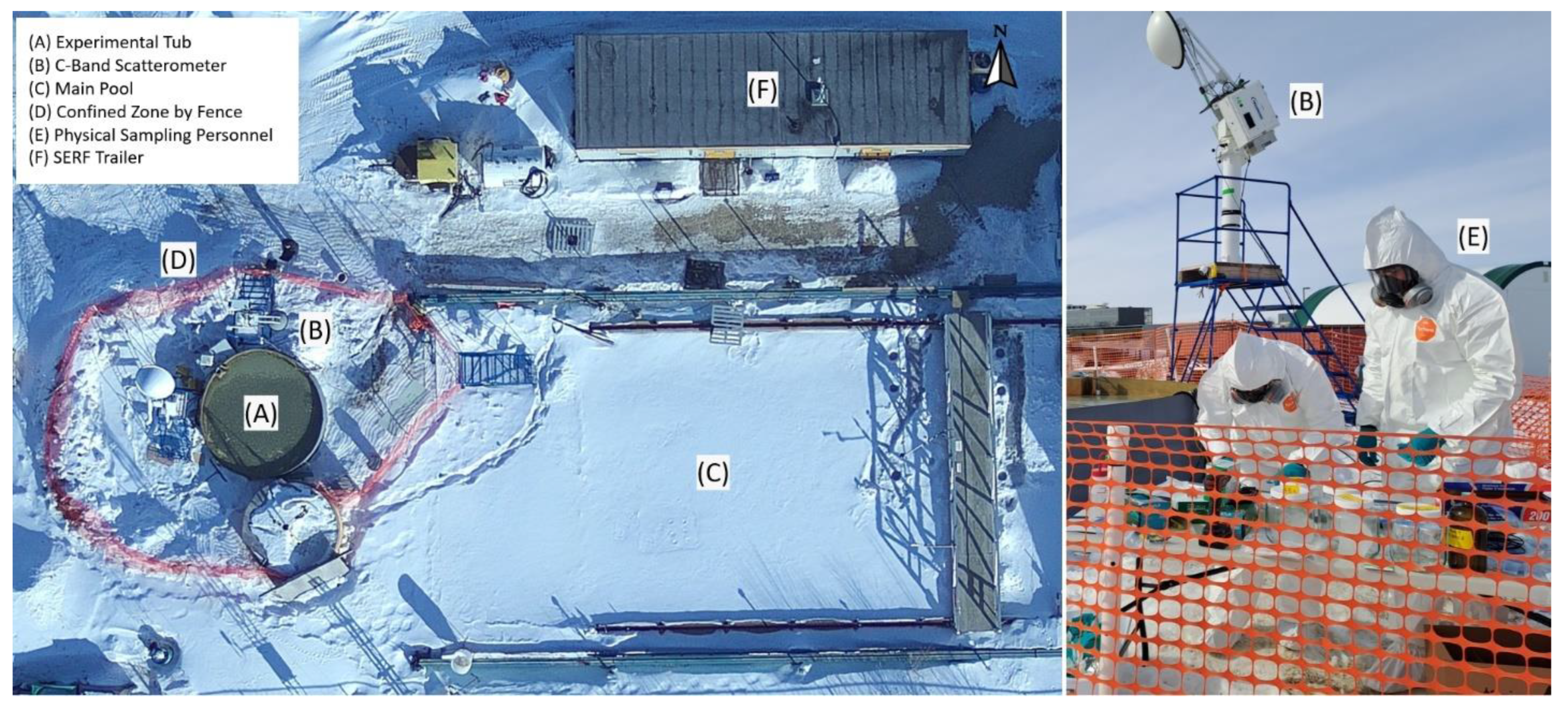
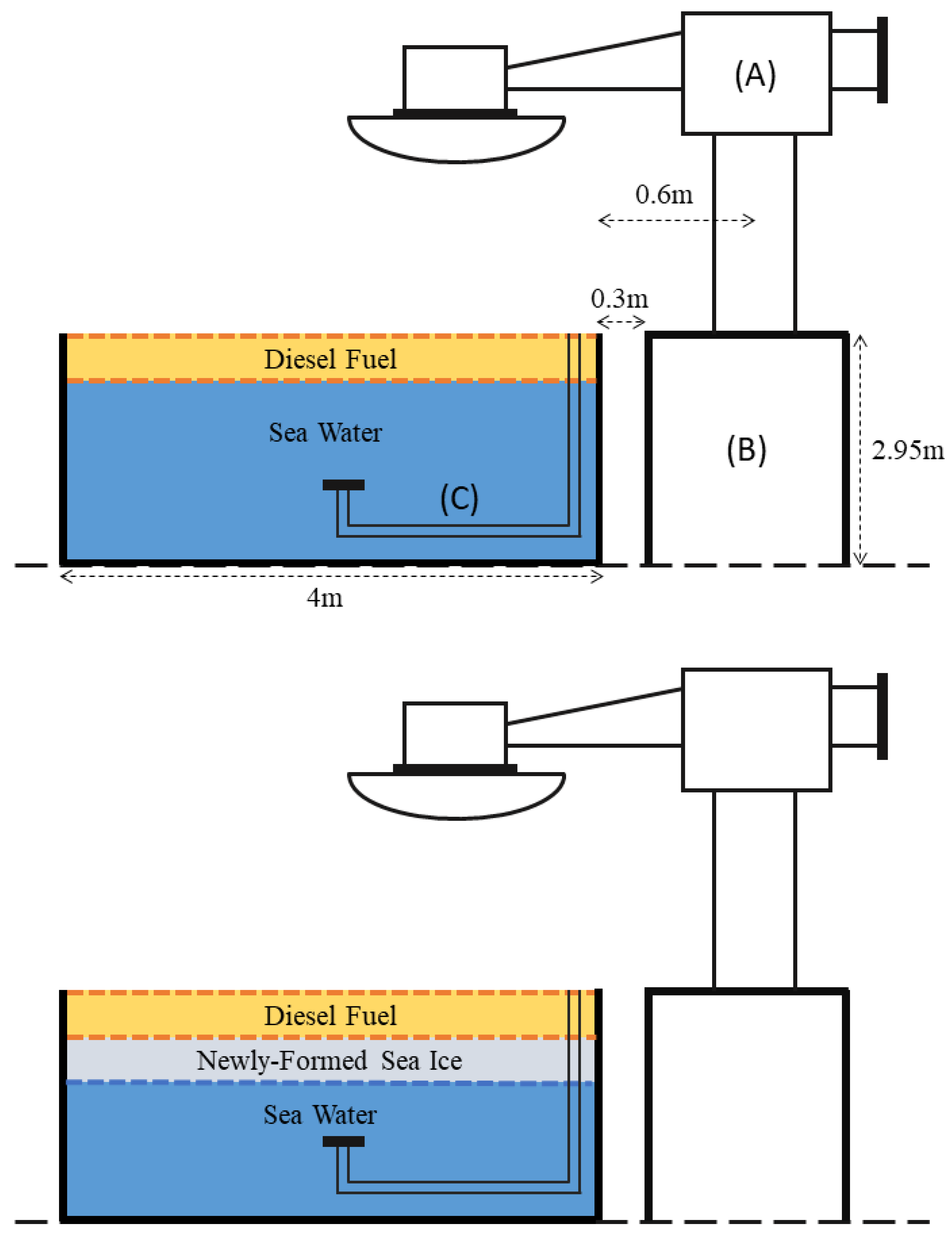
In 2023, we performed a series of diesel spill experiments, which build upon the techniques that our group has been developing over the past eight years (e.g., [24,25]). The experimental site was located at the University of Manitoba’s Sea-ice Environmental Research Facility (SERF), Winnipeg, MB, Canada. SERF is an outdoor mesocosm facility, with a main pool used for sea ice process and remote sensing studies and an adjacent set of tubs that can be filled with water from the main pool that may be contaminated in experiments. The cylindrical tub (used in this experiment) has a 4 m diameter and a 1 m depth, and it contains a noninsulated fiberglass layer. The outdoor mesocosm experiment was carried out in this cylindrical tub filled with saline water at the western side of the main pool (see Figure 1). The scatterometer was installed on a scaffold tower (2.95 m) adjacent to the tub in order to capture an overhead view. In this experiment, we focused on remote sensing of the processes that occur when a diesel spill is present on seawater and is subjected to winter conditions. The experimental period was scheduled based on when the forecast air temperatures were below 0 °C in the late winter (13–17 March). Water was transferred from the main pool after the typical formulation and mixing processes had been completed. In this experiment, the salinity of the seawater was measured at 20.9 PSU, which was notably lower than the natural Arctic Ocean surface water.
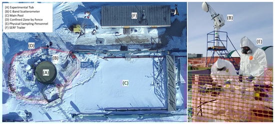
Figure 1.
The overlook of SERF and oil-spill experiment. The drone image on the left was taken before running the experiment. The photograph on the right was taken manually by a camera during a physical sampling session. (A) The cylindrical tub filled with diesel-contaminated water. (B) The C-band scatterometer installed within the confined experimental zone and adjacent to the tub. (C) The main pool that supplied the artificial seawater for the experiment. (D) Safety fence surrounding the experimental zone. (E) Personnel wearing protective clothing to perform physical samplings. (F) SERF trailer, including the equipment required to run and control the experiment.
In the initial phase of the experiment (under review), we grew sea ice and introduced 20 L of diesel beneath it (the inlet is located at the bottom of the pool). After that experiment, we reset the experiment by turning on the heaters inside the tub to melt all of the ice. Subsequently, we shut down the heaters and investigated the impacts that the diesel had on the sea ice formation procedure (similar to [24]). Concurrently, the thermophysical properties within the tub were monitored by in situ observations and physical samplings. Safety provisions were the main priority throughout the experiment and personnel involved were trained in handling oil products and using safety gear (e.g., coverall suits, passive respirators, and H2S sensors). Moreover, we placed a fence around the experimental area to indicate a confined zone for safety precautions (see Figure 1).
2.2. Scatterometer Instrumentation
During the experiment, a custom-designed C-band polarimetric scatterometer system (C-SCAT), built by ProSensing Inc., Amherst, MA, USA, was used to monitor the backscattering behavior (e.g., NRCS). C-SCAT is an active microwave radar that uses a frequency-modulated continuous wave (FMCW) with a central frequency of 5.5 GHz and a bandwidth of 500 MHz. This system is equipped with a dual-polarized parabolic antenna with a narrow beamwidth, such that the footprint of the radiation on the surface can be contained within the oil tub. The system is designed to operate over small ranges (<30 m) due to using a very low-power transmitter; however, it can measure the complex scattering matrix of the target in less than 10 ms via pulse-to-pulse polarization switching. To achieve a full scattering matrix, the antenna was set to measure radar pulses in quad-polarization states (i.e., VV, VH, HV, and HH). By averaging the backscattered samples, the multipolarization NRCS alongside several polarimetric quantities (Rco, Rxo, H, α, ρco, and μ) were calculated from the complex scattering matrix data. Table 1 provides the main specifications of the C-SCAT sensor. The scatterometer has an associated computer-based device (Getac laptop model S410) as an interface for commanding the system, configuring the scans, and storing the raw data files. Moreover, the polarimetric parameters were stored in the format of the target covariance matrix [C4]. Further details on this system and its operation have been reported in the literature [24,28,36].

Table 1.
Scatterometer operating specifications.
2.2.1. Scatterometer Data Collection
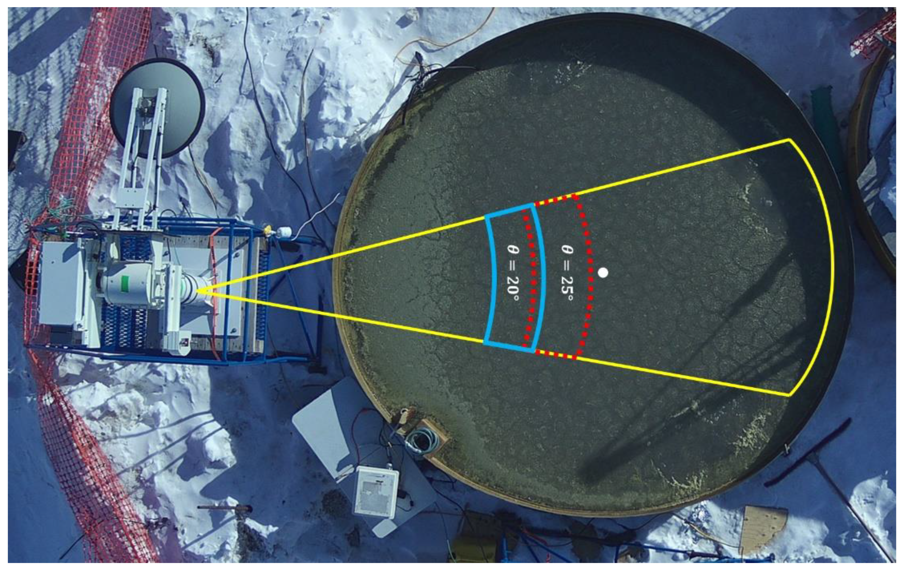
The C-SCAT was configured to collect data approximately four times per hour (each scan takes nominally 2 min, and we imposed a 15-min delay between scan stop and start). These scans were carried out as the scatterometer pivoted along the vertical and horizontal axis within the elevation amplitude of 0° to 60° (with steps of 5°) and the azimuth swath of 30°. The scanning geometries were assessed based on acquiring the radar backscattering signatures independent from the tub’s edge effect (see Figure 2). We verified the certainty of each angle using an angle finder tool, which resulted in ±0.5° accuracy. Herein, data from 20° and 25° incidence angles are presented without interference by the tub’s perimeter. To ensure that the presented measurements were not influenced by the tub edges and the surroundings, we conducted verification measurements, in which we deliberately used a wide azimuth swath and a large range of incidence angles. From the results, we established the angles for which the edges were illuminated and reduced the scan parameters to ensure that we were only measuring the water/ice surface. For example, at higher elevation angles, a persistent horizontal scattering return that corresponded to the far tub edge was seen in the range profile. Consequently, we did not provide those results herein. The instrument relies on an internal delay line calibration to monitor for system drift during operation. An external corner reflector calibration was performed, and a polarimetric calibration was applied, following the description in the manufacturer’s specification and published papers on the topic. Calibration was stable throughout this relatively short experiment. We considered the range of our data from the experiment starting on 13 March (00:00) to the experiment ending on 17 March (10:00). After that, the sea ice was subjected to intense physical sampling activity that rendered it unusable for remote sensing measurements.
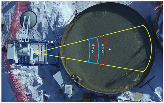
Figure 2.
Scatterometer footprint taken after the last physical sampling session on 17 March. The highlighted zones represent the swaths of selected incidence angles (20°: solid blue line, and 25°: dashed red line. The optimal angles are chosen carefully by visual inspection and geometric calculations in order to minimize the errors caused by the tub’s edge.
2.2.2. Scatterometer Data Processing
Interface description language (IDL) and MATLAB source codes were utilized to preprocess and analyze the collected CSCAT data, respectively. By recording the returned power and phase, we were able to calculate the covariance matrix, and hence, the NRCS was achieved. We took the average of HV and VH, under the assumption of reciprocity, to display the crosspolarization mode. Afterwards, a four-point rolling mean filter was applied to reduce the system noise for plotting the NRCS results. We analyzed temporal variations of NRCS using visual observations to detect significant changes and relate them to notable events during the experimental period. Afterward, the two incidence angles were compared with each other over a time-series basis. We tested several scans on a pulse-by-pulse approach to examine data quality and ensure that an adequate signal-to-noise ratio was maintained.
We calculated the backscattering ratios (i.e., Rco and Rxo) using the covariance matrix [C4]. The C4 was reduced to a 3 × 3 averaged matrix [C3] for a monostatic configuration (see Equation (1)). Consequently, we were able to derive other polarimetric parameters (i.e., µ, , and H) (see Equations (2)–(7)). As suggested by [25], the conformity coefficient (µ) was selected as a parameter to investigate since it is highly sensitive to surface roughness. The µ parameter ranges between −1 and +1 values. It distinguishes between smooth and even very slightly rough surfaces by appointing them negative and positive values, respectively. According to Equation (3), µ contrasts the correlation between co- and crosspolarized scattering responses. We also used Cloude’s eigen-based decomposition, one of the TD theorem methods, to calculate H and α parameters from the coherency matrix and attain natural terrain classification [32]. From this, the homogenous level of sea ice, known as surface scattering low entropy (SSLE) [37], can be classified. The SSLE, alongside the other seven zones, were previously defined by investigating the polarimetric SAR imagery of various natural terrains [32,38]. We followed this classification process for an oil-contaminated, sea-ice scenario, knowing that the medium’s scattering inhomogeneity and the dominant scattering mechanism are associated with H and parameters, respectively [32].
2.3. Meteorological Observations and Physical Sampling
Due to the size limitations of the mesocosm, we performed three discrete in situ physical sampling sessions, which allowed us to budget the sampling space without disturbing the radar footprint. The dates of sampling sessions and type of measurement activities can be found in Table 2. During each session, three sites were investigated. The sampling sites were selected carefully so that their locations did not coincide with the scatterometer scan footprint (see Figure 3). We completed this stage by collecting diesel fuel and seawater samples on all sampling dates. Ice sampling was performed on 17 March when a thin layer of ice was observed.
Table 2.
Sampling types at different sessions.
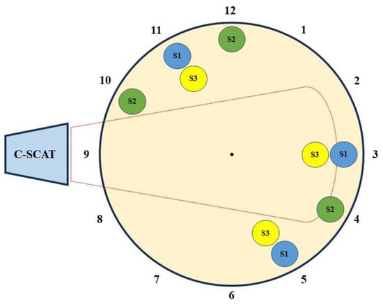
Figure 3.
Physical sampling locations. The locations were digitized based on a clockwise system. S1: Sampling session 1 (13 March-Blue), S2: Sampling session 2 (14 March-Green), S3: Sampling session 3 (17 March-Yellow), dashed red perimeter: C-SCAT scan region.
Meanwhile, meteorological parameters such as air temperature and relative humidity were recorded by a local weather station located 15 m away from the tub. The wind speed data were collected from the “Winnipeg INTL A” weather station (with the nearest proximity to SERF) via the Environment Canada website. The recorded meteorological data were processed through filtering, and their results also were displayed via MATLAB (academic version R2022b, developed by The MathWorks, Inc., Natick, MA, USA).
2.3.1. Sample Collection
A set of bulk ice samples with rectangular dimensions was collected by cutting the ice layer with a hand bone saw. Additionally, the ice surface was sampled by scraping the ice with ~0.5 cm thickness using metal spatulas. We measured the thickness of each extracted bulk ice sample before placing them in prebaked 2 L transparent glass jars. Moreover, the Kim wipe test was applied to determine the presence or absence of moisture on the sea ice surface. The diesel layer was sampled carefully with disposable glass Pasteur pipettes and collected in 100 mL cleaned and baked amber glass jars. Additionally, the water (1 L sample) below the diesel layer was collected at different depths (see Table 3) using a peristaltic pump. The diesel layer samples taken during the 13 and 14 March were stored in the fridge. Only the samples that contained sea ice (collected from cores and scrapings on 17 March) were stored in the freezer.
Table 3.
Physical sampling results.
2.3.2. Sample Processing
Diesel-contaminated sea ice (from 17 March) and open water diesel layer samples (from 13 and 14 March) were stored in freezer (−15 °C) and fridge (+4 °C) temperatures, respectively. Liquid bulk diesel was pipetted from the surface of intact ice samples and measured volumetrically in a glass graduated cylinder. Frozen samples were then allowed to thaw at room temperature. The total volumes (VT) of all samples (melted and originally liquid) were measured volumetrically using glass graduated cylinders. Any observable diesel layer on the water surface inside the graduated cylinder was noted for its volume (VDiesel) and was subsequently removed from the surface with a glass Pasteur pipette. The oil volume fraction was determined by VDiesel/VT. (The accuracy and limit of detection for the various volumetric measurements are provided in Table 4.) The remaining water fractions were then measured for their conductivity and practical salinity using a Cond 3310 m equipped with a TetraCon 325 measuring cell. This device was calibrated with a calibration standard (0.01 mol/L KCl) for conductivity cells. The reference salinity was calculated from the measured practical salinity using Equation (8), where SR is reference salinity (g/kg), and SP is practical salinity (unitless) [39].
Table 4.
Volumetric measurement information.
3. Results
3.1. Experiment Overview
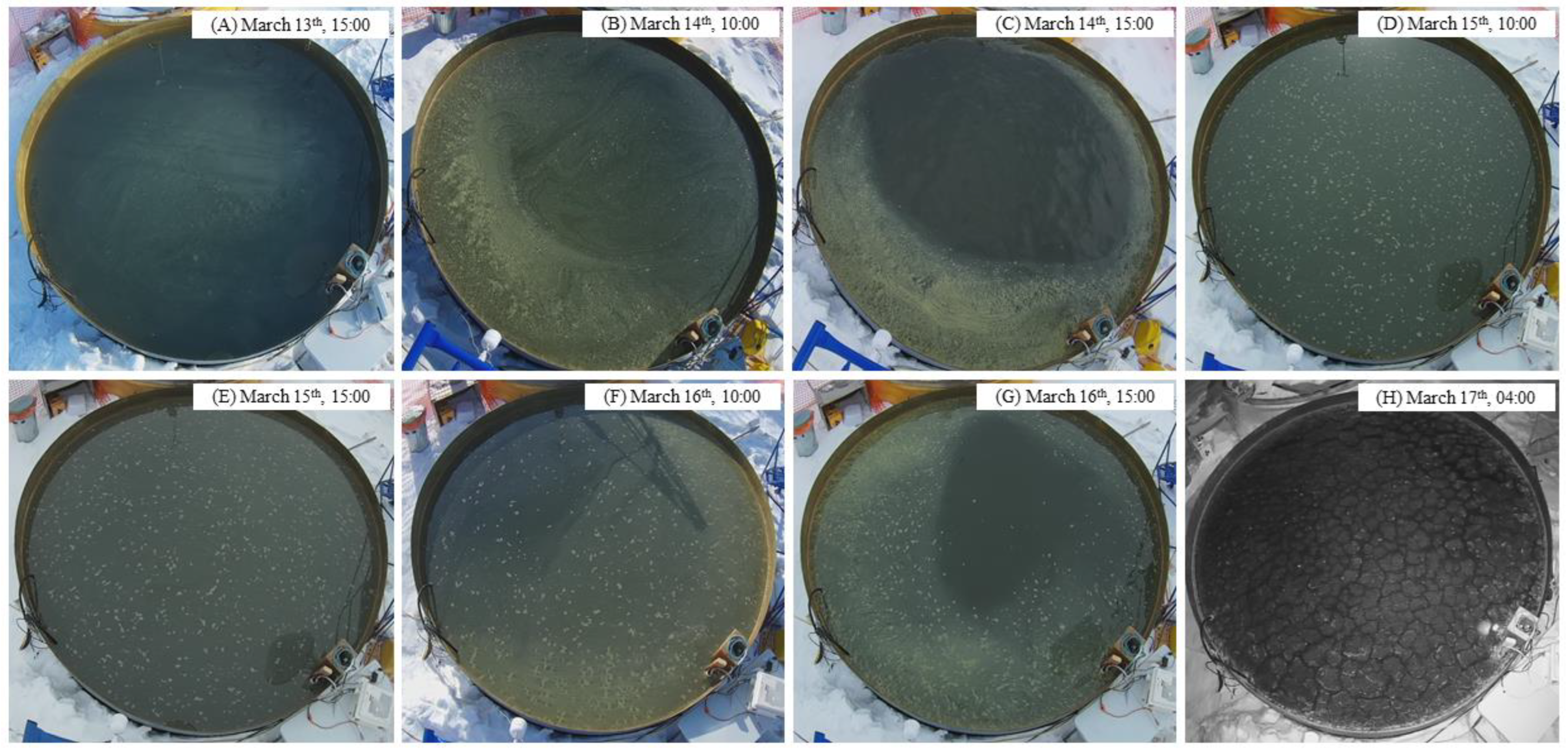
The experiment began with ~20 L of diesel floating on seawater. Monitoring procedures were started on 13 March, a day after the heaters were turned off on 12 March. Although the air temperature remained below 0 °C and strong winds blew during the study period, the sea ice only appeared visibly after 17 March (2.7 cm average). These conditions allowed us to section the experimental period into three stages: (1) diesel on seawater: under a calm condition (13 March, 00:00–14 March, 15:00), (2) diesel on seawater: under strong windy conditions (14 March, 15:00–17 March, 04:00), and (3) diesel on formed sea ice (after 17 March, 04:00) under slight windy conditions. Photographs in Figure 4 were captured automatically by a camera attached to the scatterometer post. They represent the time-series progression of the sea ice growth from the same looking angle upon the tub. During the 13th and 14th of March, the tub faced having diesel as the topmost layer (3 mm thick), a dirt interface layer (which was too thin to be collected), and water beneath the diesel layer. The described structure is shown as a diagram in Figure 5. However, the windy conditions played a substantial role in distributing the diesel layer. After each maximum wind speed (two major maxima on 14 March and 16 March in corresponding to Figure 4B,G), a large part of the floating diesel was pushed to the sides. These phenomena were followed by the appearance of several light spots on top of the diesel layer (Figure 4D–G). Eventually, a 3 mm diesel fuel ice slushy layer was observed on 17 March (see Figure 4H as well as the regenerated diagram in Figure 5). Furthermore, Table 2 presents various types of physical samplings that we performed during this study. The diesel and water physical characteristics were measured throughout the experiment, while sea-ice thermophysical properties were attained only on the last sampling date (17 March). The list of sampled quantities and their results are shown in Table 3.
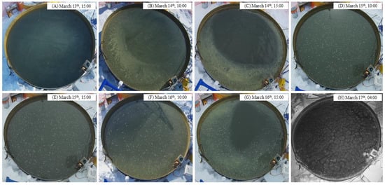
Figure 4.
Temporal progression of sea ice growth within the diesel-contaminated tub. The alphabetic marks are set to assign photographs to sync radar signatures. (A) Open water (no ice) with diesel as the topmost layer under a relatively calm condition a day after heaters were turned off. (B) Open water (no ice) with diesel nearly shifted to the edges under a strong, windy condition. (C) Open water (no ice) with diesel almost entirely pushed to the sides while the maximum wind speed was dominant. (D,E) Open water (no ice) with multiple light spots under a calmer condition. (F,G) The diesel layer and light spots move around at a lower rate of wind speed. (H) Slushy layer of diesel fuel and ice with light and dark spots.

Figure 5.
Experimental tub diagrams before and after the ice formation. (A): C-band scatterometer, (B): Scaffold tower, (C): Oil pipe.
3.2. Meteorological Results
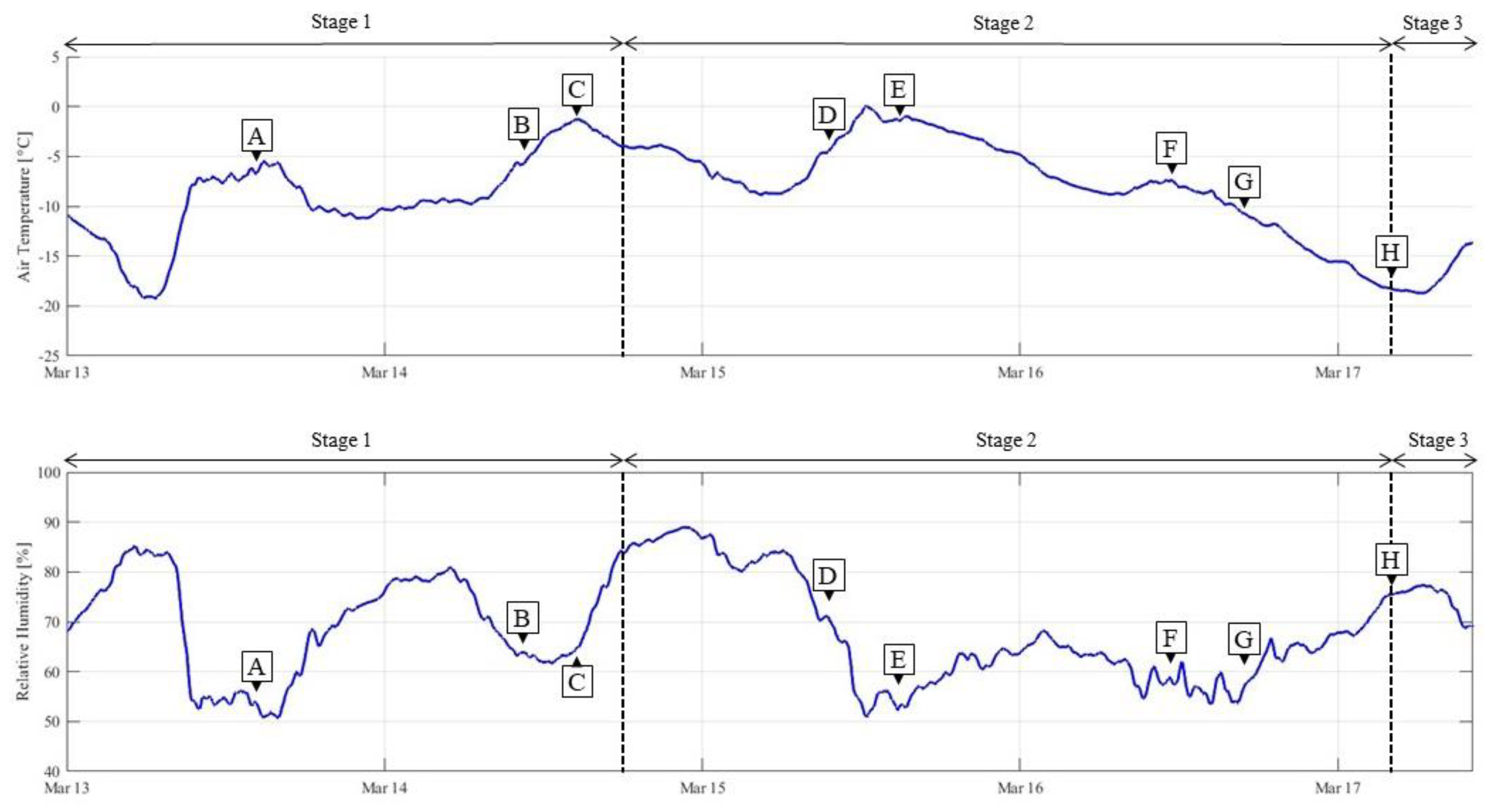
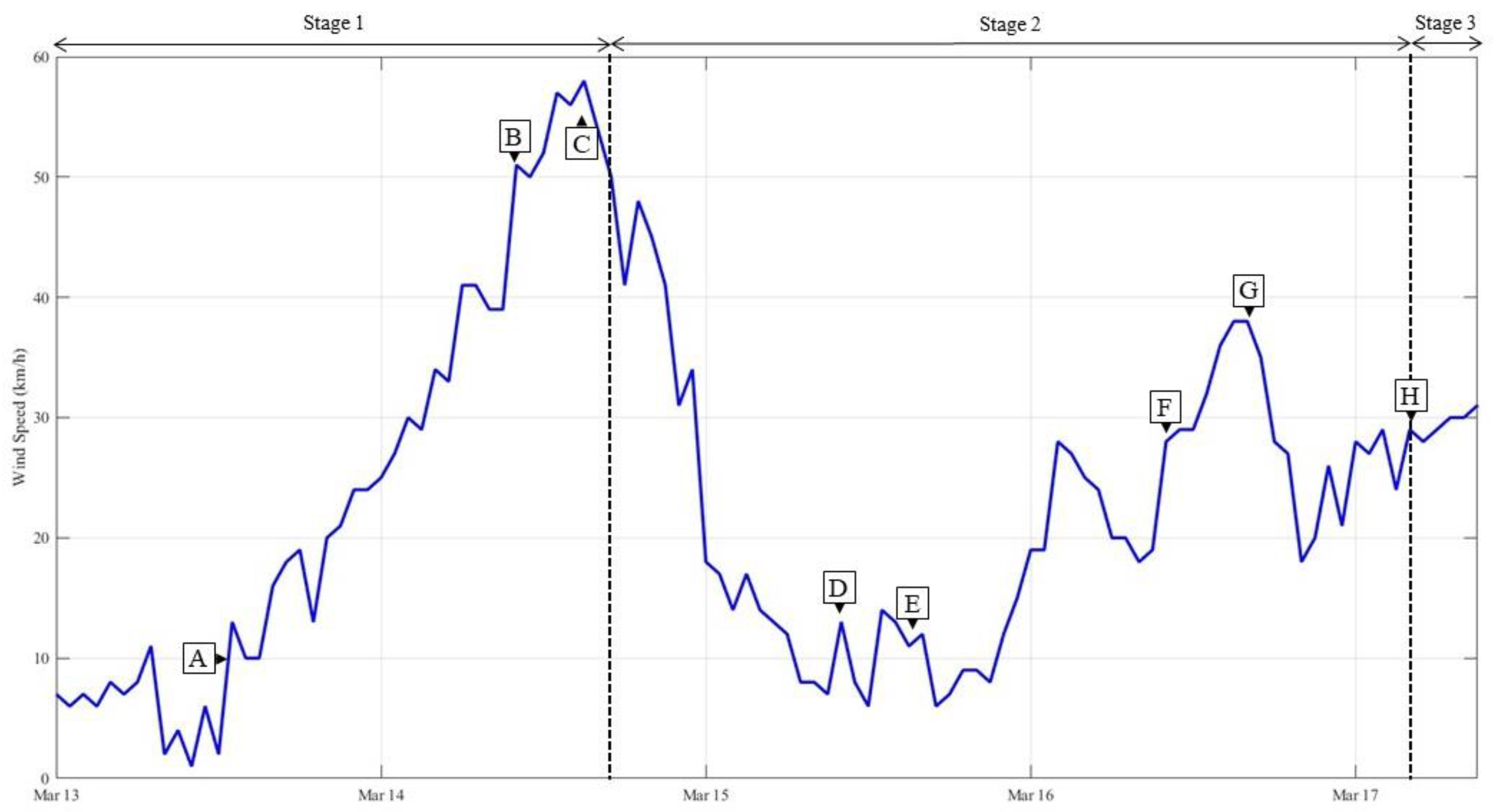
During the experimental period, the air temperature stayed below 0 °C and oscillated within the amplitude of 19 °C. The minimum temperature was −19 °C on 13 March at 07:00, and the maximum was 0 °C on 15 March at 13:00. The relative humidity varied in the range of 38% (with a minimum of 51% and a maximum of 89%). Both meteorological parameters followed a diurnal cycle of change throughout the study period (See Figure 6). During Stage 1 of the experiment, the air temperature started from approximately −11 °C and leapt down to −19 °C at 07:00 on 13 March. Thereafter, the air temperature rose towards −2 °C. During Stage 2, the air temperature reached 0 °C and then followed a downward trend. After Stage 3 started, it reached −18.7 °C around 07:00 on 17 March and then slightly increased (with a relative humidity of 77%). Moreover, it is crucial to mention that our study was being synchronized with several windy days. The temporal variation of the wind speed during the experiment is presented in Figure 7. Stage 1 started with a relatively calm condition. The lowest rate of wind speed was reported at 3 km/h at 08:00 on 13 March. From there on, the wind started to grow and reached its highest speed (58 km/h) at 15:00 on 14 March. Stage 2 began with wind speed reaching its first maxima. However, it decreased drastically after and continued on average at 11.3 km/h on 15 March. Subsequently, the wind grew again and reached 38 km/h on 16 March. At last, the meteorological measurements were finished before the last sampling session at 10:00 on 17 March when the air temperature was −14 °C and the wind condition was comparably calmer. We expect the wind speed values to be relatively lower at the tub surface since the wind speed decreases with reducing altitude. Nevertheless, the wind played a key role in our analysis, as it notably affected the NRCS and polarimetric results, which we will fully describe in the upcoming sections.
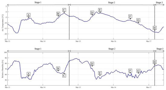
Figure 6.
Time-series variation of air temperature (°C) and relative humidity (%) during the experiment. The length of each stage is specified by horizontal lines and separated by vertical bars. Figure 4 (the temporal progression of sea ice growth within the diesel-contaminated tub) has been linked to these results by its (A–H) alphabetical marks. Stage 1 was open water, Stage 2 was open water under strong windy conditions, and Stage 3 had sea ice under slight windy conditions.
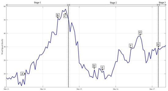
Figure 7.
Time-series variation of wind speed (km/h) during the experiment. Data reported from “Winnipeg INTL A” weather station located at Winnipeg Richardson International Airport, Manitoba, Canada. The length of each stage is specified by horizontal lines and separated by vertical bars. Figure 4 (the temporal progression of sea ice growth within the diesel-contaminated tub) has been linked to these results by its (A–H) alphabetical marks. Stage 1 was open water, Stage 2 was open water under strong windy conditions, and Stage 3 had sea ice under slight windy conditions.
3.3. NRCS Results
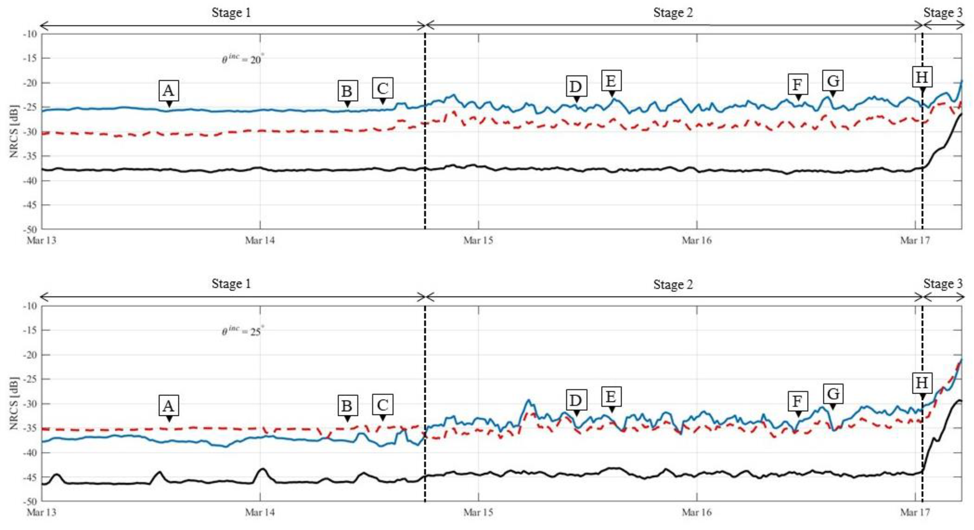
Figure 8 presents the temporal responses of C-band multipolarization NRCS at 20° and 25° incidence angles. We calculated and presented in Table 5 the average and the standard deviation of cross- and copolarization states for each stage in both incidence angles. As expected, the NRCS signatures at 20° were several dB higher than at 25°. During Stage 1, all NRCS states (i.e., HH, VV, and HV) were relatively stable at 20° and 25°. While the windy conditions were dominant over Stage 2, copolarization responses (HH and VV) started to ripple in both incidence angles. However, NRCS at 25° behaved differently, as VV stood lower than HH during Stage 1. From Stage 2 forward, it rose from −38 dB to −33 dB and settled higher upon HH. This behavior was continuous until the ice layer was created in Stage 3. After sea ice formed, we observed significant increases in HH, VV, and HV values. Meanwhile, the crosspolarization responses, represented as HV, remained comparatively stable and lower than the copolarization states in both incidence angles throughout the experimental period. However, crosspolarization signals exhibited more fluctuations at 25° compared to the 20° incidence angle, particularly along Stage 2.
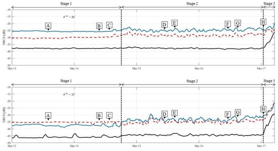
Figure 8.
Time-series multipolarization responses of normalized radar cross section (NRCS) at 20° and 25° incidence angles. VV: solid blue line, HH: red dashed line, HV: solid black line. The length of each stage is specified by horizontal lines and separated by vertical bars. Figure 4 (the temporal progression of sea ice growth within the diesel-contaminated tub) has been linked to these results by its (A–H) alphabetical marks. Stage 1 was open water, Stage 2 was open water under strong windy conditions, and Stage 3 had sea ice under slight windy conditions.
Table 5.
NRCS calculations.
3.4. Polarimetric Parameter Results
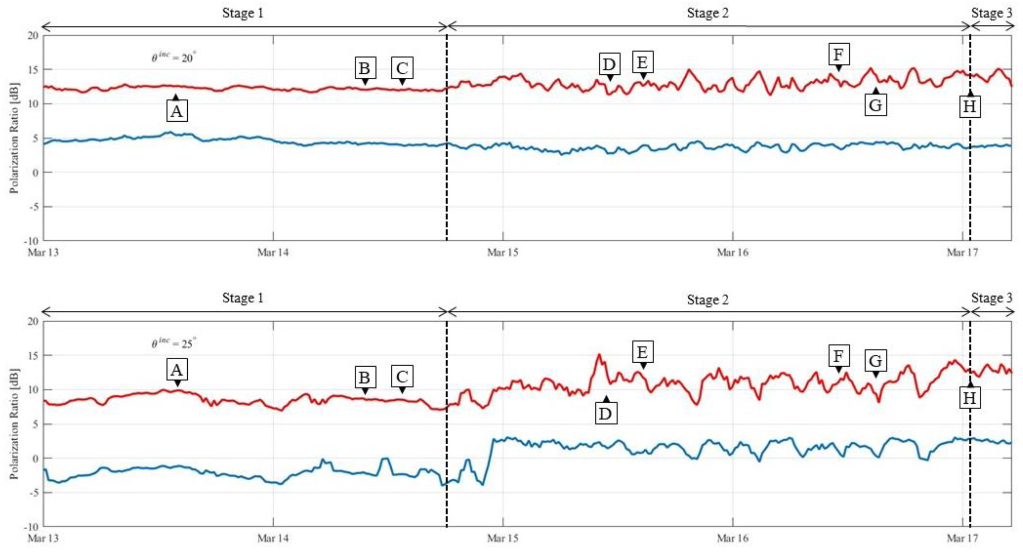
We presented the temporal variations of backscattering ratios (Rco and Rxo) alongside their average and standard deviations (STD) in Figure 9 and Table 6, respectively. According to Figure 9, the Rxo is >10 dB for both incidence angles. The Rco at 20° was nominally 5 dB with much lower signal levels for the 25° incidence angle. The Rco and Rxo parameters in 20° and 25° incidence angles were consistent during the calm condition of the diesel layer upon seawater within Stage 1. However, this consistency at 25° was lower than the 20° incidence angle as it showed more fluctuations. As time progressed (during Stage 2 and gusty conditions), both Rco and Rxo signals began to exhibit oscillatory behaviors. Likewise, in Stage 1, the oscillation amplitudes at the 25° incidence angle (~8–15 dB) were greater than the oscillation amplitudes at the 20° incidence angle (~11–15 dB). Furthermore, the Rxo parameter demonstrated more intense oscillations than Rco signals. Eventually, both polarization ratios (Rco and Rxo) stabilized after sea ice was formed at Stage 3.
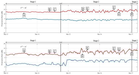
Figure 9.
Time-series responses of Rco and Rxo for incidence angle 20° and 25°. Rxo: red line, Rco: blue line. The length of each stage is specified by horizontal lines and separated by vertical bars. Figure 4 (the temporal progression of sea ice growth within the diesel-contaminated tub) has been linked to these results by its (A–H) alphabetical marks. Stage 1 was open water, Stage 2 was open water under strong windy conditions, and Stage 3 had sea ice under slight windy conditions.
Table 6.
Backscattering ratio calculations.
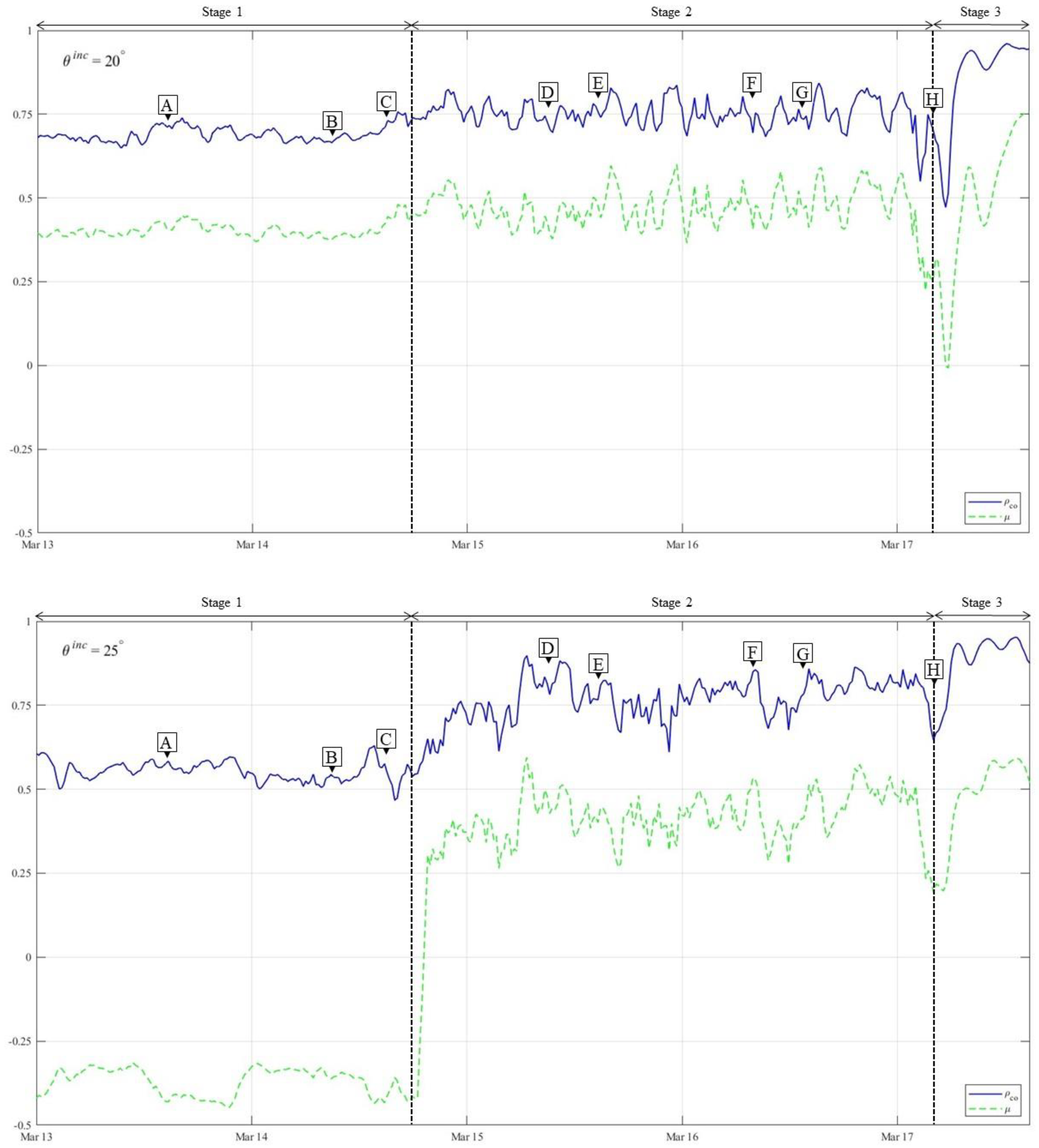
Polarimetric parameters, namely μ and ρco, are presented in Figure 10. At the 20° incidence angle, the μ parameter progressed above zero and remained stable (~+0.4) from Stage 1 until the outset of windy conditions. After the gust reached its highest speed around 15:00 on 14 March (beginning of Stage 2), the μ parameter demonstrated an oscillatory trend. The amplitude of changes fluctuated between +0.4 and +0.6 continuously prior to the formation of sea ice on 17 March at 04:00. In Stage 3, the μ parameter faced a considerable plunge and reached its minimum value around 0. On the other hand, μ at a 25° incidence angle exhibited a transitory trend from negative to positive values in the transition from Stage 1 to Stage 2. When the windy conditions prevailed in Stage 2, the μ parameter had a significant abrupt uplift from −0.4 to +0.3 and thereafter, kept oscillating within the range of +0.3 and +0.5. A similar plunge, but with a lower depth, was noticed slightly earlier than the 20° incidence angle, as the tub observed sea ice and entered Stage 3. The ρco parameter in Stage 1 progressed relatively stable in both incidence angles. Stage 2 at the 20° incidence angle showed a minor derivation to the windy condition. In Stage 2 at the 25° incidence angle, however, ρco responses were stronger with a sharp increase (from +0.5 to +0.85), which can be observable with the transitory change of μ. Both ρco and μ parameters appeared to follow the same downward and upward trends. In response to the sea ice formation during Stage 3, the ρco and μ parameters initially demonstrate a downward trend. The reduction was greater in the 20° incidence angle, as the ρco parameter decreased from 0.75 to 0.47 and the μ parameter decreased from 0.28 to 0. In comparison, at the 25° incidence angle, the ρco parameter decreased from 0.80 to 0.64, and the μ parameter decreased from 0.42 to 0.19.
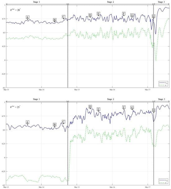
Figure 10.
Time-series responses of μ and ρco for incidence angle 20° and 25°. ρco: blue line, μ: green dashed line. The length of each stage is specified by horizontal lines and separated by vertical bars. Figure 4 (the temporal progression of sea ice growth within the diesel-contaminated tub) has been linked to these results by its (A–H) alphabetical marks. Stage 1 was open water, Stage 2 was open water under strong windy conditions, and Stage 3 had sea ice under slight windy conditions.
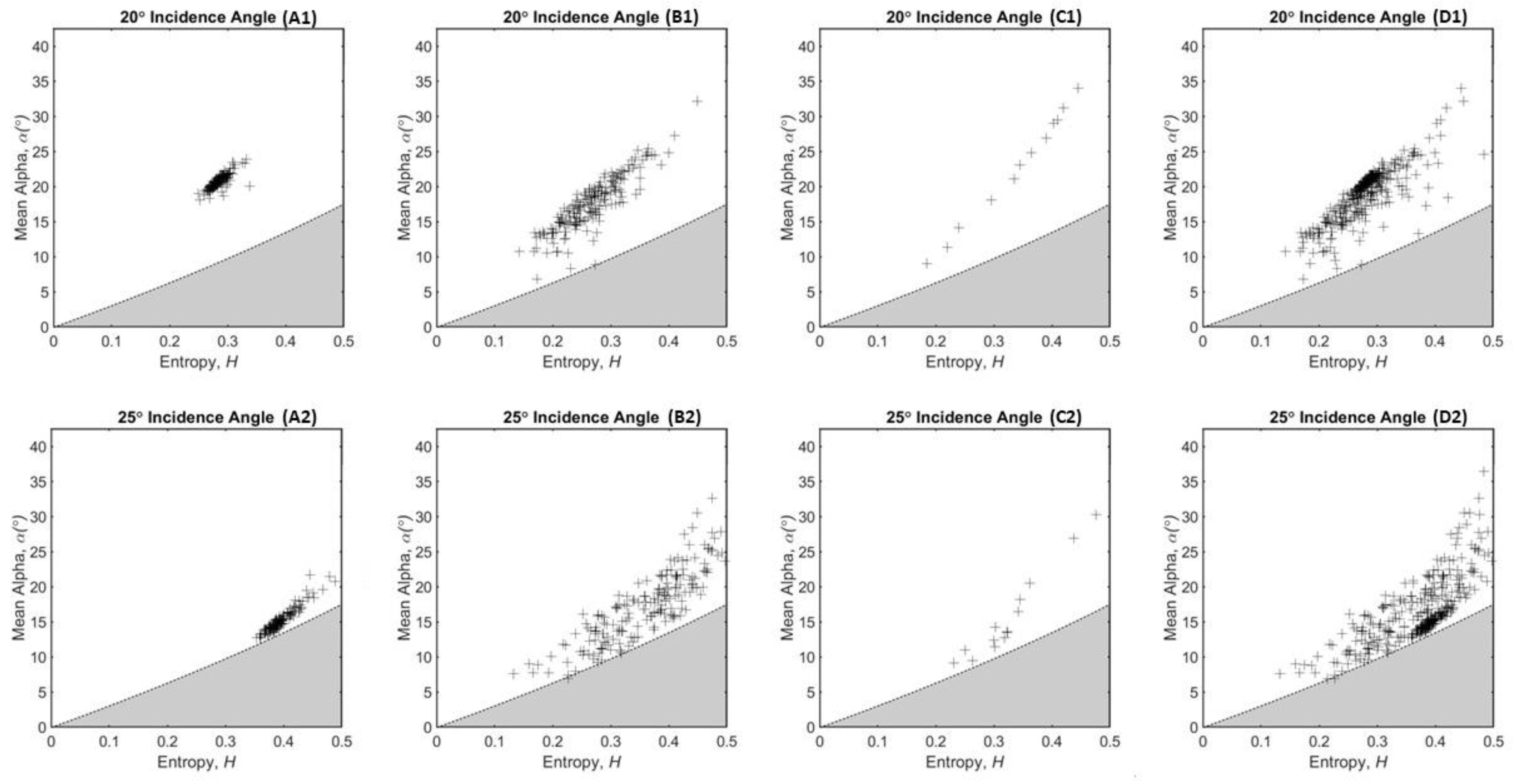
We generated scatterplots of H (entropy) versus α (mean-alpha), as shown in Figure 11. The H/α scatterplots exhibit the distribution of measurement points (clusters) throughout the study period. The mean values of H and α were calculated to locate the concentration of clusters accurately. Each cluster specifies a diesel fuel-free or diesel fuel-contaminated regime within the tub. During Stage 1, scatterplot A1 at the 20° incidence angle showed that clusters are mostly concentrated at H = 0.28 and α = 21° within the SSLE zone. However, in Stage 2, clusters in scatterplot B1 showed a very high dispersion from the lower left corner to the upper right corner. This trend was followed as well during Stage 3 (scatterplot C1) when ice was present at the end of the experiment. The overall distribution of clusters is presented in scatterplot D1, and it shows the clusters are mainly congregated around H = 0.28 and α = 21°.

Figure 11.
Scatterplots of H (entropy) versus α (mean-alpha). (A1,A2): Open water (no ice) under calm conditions (Stage 1). (B1,B2): Open water (no ice) under strong windy conditions (Stage 2). (C1,C2): The presence of sea ice under slight windy conditions (Stage 3). (D1,D2): Distribution of clusters throughout the study period (from 13 March (00:00) to 17 March (10:00)).
The distribution of clusters at a 25° incidence angle was different. With open water in Stage 1, the measurement points fell over H = 0.39, and α = 15° (scatterplot A2). During Stage 2, clusters in scatterplot B2 distributed in a different position and exhibited more dispersion than the clusters at a 20° incidence angle. After sea ice formed in Stage 3 (scatterplot C2), the distribution of clusters was similar to 20° (scatterplot C1), as it also dispersed from the lower left corner to the upper right corner. The overall distribution of clusters at the 25° incidence angle (scatterplot D2) shows that clusters are mainly located around H = 0.39 and α = 15°. At the 25° incidence angle, scatterplot D2 demonstrates higher variability than scatterplot D1 at 20°. In an overall view, clusters in both incidence angles are scattered linearly in the same direction. This behavior appears mostly in Stage 3 and at a 20° incidence angle (scatterplot C1).
4. Discussion
The vision of this study was focused on answering two questions: (1) “How does the presence of diesel fuel and wind upon seawater alter the growth, thermophysical, and microwave C-band scattering behaviors of newly forming sea ice?” and (2) “Which polarimetric parameters are most sensitive to the presence of diesel fuel on newly formed sea ice?” We described the collected datasets and their associated figures in the results section. Here, we present discussions based on our interpretation of the results. Discussions will be divided into the following categories: (1) Physical sampling, (2) NRCS, and (3) Polarimetric parameter analysis.
4.1. Physical Sampling
The experimental scenario was carried out during expected winter conditions in Winnipeg, Canada. The air temperature remained at the freezing level (below 0 °C) throughout the study, providing a situation for sea ice growth. Regarding Table 3, the surface temperatures of both water and diesel decreased as we turned off the heaters. Windy conditions were dominant in the midst, which divided our experiment into three stages (as previously defined in Section 3.1). With the recorded wind speed, a pancake ice formation might be expected [13]. Interestingly, the newly forming sea ice broke into segments, rather than growing under a purely quiescent form (see Figure 4H). However, it appears that the wave-dampening effect of the diesel layer over top of the ice segments has prevented the typical rims and ridges of pancakes from forming. This is important, as it indicates that ice formation beneath a layer of diesel is similarly affected by wind, as observed in [40]. Further study of this result is required, as the oil tub is a small volume of water, and large-scale natural effects, such as wind fetch and water circulation, are not addressed. When the gusting winds were dominant, they disturbed the surface and prevented diesel from being a smooth layer (see Figure 4B,C,F,G). Although the wind speed was not strong enough to make waves, the continuous windy conditions on 14 March and afterward increased the roughness of the diesel surface by creating small ripples. Oil weathering is known to be enhanced under windy conditions [40]. Therefore, it created an emulsion layer by making more water come to the surface where it mixed with the diesel fuel. Moreover, the variability of targets was observed in the radar field of view. This could be explained as the diesel fuel used in this experiment is relatively light (i.e., ρ = 0.85 g/mL (25 °C)) and hence, moves fast on the wind-ridden surface. Based on all these factors, Stage 2 was separated from Stage 1 and Stage 3 since the other two stages had calmer conditions.
As previously mentioned, in this experiment, the seawater salinity was 20.9 PSU. After the ice was formed, the salinity of water slightly increased (~21.2 PSU). However, the salinity of the surface slush (mixture layer of ice and diesel) was recorded to be significantly higher (~32.0 PSU). Brine expulsion to the surface of sea ice is a well-documented phenomenon (e.g., [28,41,42]). The physical properties of a diesel infiltrated slushy layer on a sea ice surface are relatively unstudied and this work provides results for this oil spill scenario.
4.2. NRCS Analysis
We investigated the results of multipolarization NRCS responses to answer our first question: “How does the presence of diesel fuel and wind upon seawater alter the growth, thermophysical, and microwave C-band scattering behaviors of newly forming sea ice?”
Figure 8 demonstrates the time-series NRCS responses from multipolarization CSCAT. As it has also been illustrated by [24,25] (for oil), the NRCS signals progressed in a relatively stable state, whereas a smooth layer of diesel fuel covered the seawater in Stage 1. However, the windy conditions that were prevalent during Stage 2 enhanced the surface roughness. At times of heavier winds, ripples were evident on the water surface, whereas other times showed a smoother surface. The variety of surface roughness resulted in oscillations in NRCS responses. The wind also enhanced the surface mixing, which caused water underneath to mix with the diesel layer. Since water has a lower viscosity than diesel, the formed emulsion had greater surface roughness made by wind. These outcomes can be the possible explanations for the rippling behavior of signals in Stage 2.
Eventually, all three states of the NRCS responses (VV, HH, and HV) illustrated a notable increase when Stage 3 began. These characteristics can be attributed to the formation and presence of sea ice underneath the diesel layer. Furthermore, based on comparing STD values of stages between two incidence angles (see Table 5), it seems that the radar signals at 25° are more sensitive than the signals at 20° in detecting the presence of wind, seawater, and sea ice.
Interestingly, the VV/HH ratio in Stage 1 was positive for the 20° incidence angle and negative for 25° (implying HH > VV for Stage 1, Figure 8). These behaviors were unchanged until the presence of wind in Stage 2 made two copolarized signals back to their typical places for open water conditions, with VV > HH. A multilayer scattering model indicates that this polarization reversal is plausible for the given conditions [43,44]; however, we plan to address further modeling studies in future work. Earlier studies revealed that the multipolarization NRCS responses remained steadily stable throughout the experiment under calm conditions (see [24,25]). Several environmental and physical conditions in our experiment were dissimilar. Besides the wind, which created a turbulent situation at the topmost layer, two other elements also participated to differ our study from previous experiments. One element was the substance we used to contaminate the seawater. In this study, we used diesel fuel, one of many petroleum derived products, instead of using crude oil. In previous investigations [24,25], crude oil was added to the tub and the NRCS values fell slightly lower in comparison with our current study with a similar incident angle (25°). The other element was the salinity of artificial seawater. Comparatively, the measured seawater salinity in our scenario was lower than in the previous cases. Less saline water has a lower density, and therefore, it freezes up sooner than the higher saline water. These properties can be linked to the Arctic areas close to freshwater estuaries as well as precipitation to the surface of the Arctic Ocean. After all, the results of this study can provide a discernible contrast between diesel fuel contamination and crude oil contamination within sea ice. This is important, as it can lead to further development of the NRCS approach in detecting sea ice growth underneath the oil/fuel layer and mitigating safety risks for vessel navigation.
In summary, we observed low NRCS levels for both 20° and 25° incidence angles in Stage 1, when the winds were calm. In Stage 2, variability was observed due to the wind motion, movement of diesel, and emulsification of the water and diesel. For Stage 3, we saw a pronounced increase in the NRCS for all polarizations, which is similar to observations of newly forming sea ice, even without oil contamination.
4.3. Polarimetric Parameter Analysis
We investigated both volume and surface scattering aspects of sea ice in order to answer our second posed question of this study: “Which polarimetric parameters are most sensitive to the presence of diesel fuel on newly formed sea ice?” We examined a set of polarimetric parameters, including Rco, Rxo, , ρco, H, and α.
Regarding Figure 9, the temporal variations of Rco and Rxo parameters in 20° and 25° incidence angles depict that these ratios show a stable response during Stage 1, while a calm diesel layer masks the surface (similar to [24]). This behavior can be justified by the specular scattering mechanism caused by the smooth layer of diesel. In Stage 2, Rco and Rxo in both incidence angles responded notably to the diesel surface turbulence caused by wind. Therefore, they are effectively sensitive at the C-band frequency for detecting windy conditions. This sensitivity is even greater at 25° since the ratio changed from negative to positive, and furthermore, the ratios exhibit higher variability. However, when the windy conditions became slightly calmer during Stage 3 and a calm layer of diesel covered the surface, Rco and Rxo became stabilized again. This illustrates that neither ratios at 20° nor 25° incidence angles are adequately informative at the C-band frequency for detecting sea ice beneath the diesel layer. Furthermore, comparing standard deviations of the ratios (Table 6) demonstrates that Rxo exhibits more sensitivity than Rco to the changes happening within the tub.
Polarimetric parameters, ρco, and μ, are presented in Figure 10. In comparison with the second phase of the oil spill scenario in the previous study [25], other polarimetric parameters (ρco, and μ) behaved similarly during Stage 1 of our experiment (see Figure 10). At a corresponding angle (25°), ρco is positive (around +0.6) and μ is negative (around −0.4), respectively (similar to [25]). However, at 20°, the μ parameter has a positive value. Since positive μ values correspond to slightly rough ice surfaces [45], this result can be interpreted as μ is more sensitive to the surface roughness at lower incidence angles.
Stage 2 had significantly stronger winds than Stage 1. At the beginning of Stage 2, μ at 25° started from negative values (−0.4) and transitioned to positive values (+0.3) in response to the roughness and windy conditions. Meanwhile, ρco experienced a significant change, as it increased from 0.5 to 0.85. This rate of change was significantly lower at 20° (from +0.7 to +0.8). Hence, ρco at 25° showed more sensitivity to the surface roughness caused by wind. As time progressed, both ρco and μ parameters exhibited oscillatory behaviors. After the windy conditions prevailed in Stage 2, μ and ρco began to oscillate in both incidence angles. This can be interpreted that μ and ρco are both sensitive to the wind effects and the roughness of the surface made by it. From this, the μ and ρco parameters demonstrate unique behaviors, which were different from the previous study [16]. An important implication is that we can use μ to identify a change from calm, open water with diesel to a scenario where wind and emulsification are prevalent. However, with the differences in the incidence angles, further studies to evaluate the limitations of these results are needed.
During Stage 3, a rapid drop in μ and ρco, followed by a recovery to levels slightly higher than Stage 2, was observed in response to the presence of newly formed sea ice. The plunges of μ and ρco at 20° were stronger than 25°. Therefore, the μ and ρco parameters at lower incidence angles are more sensitive to the initial sea ice formation. Another notable aspect is that both ρco and μ quantities depicted similar upward and downward behaviors. These behaviors are novel, to the best of our knowledge, since in a previous study [25], which used crude oil as the contaminant, the μ quantity remained on the analog negative level (−0.4), and ρco stabilized around +0.5 throughout the study period. Therefore, μ and ρco can be considered for efficiently discriminating between ice-free and diesel-contaminated ice, as well as the presence or absence of wind within the environment. The rapid transient behavior (which occurred over a period of less than 2 h) suggests that frequent remote sensing measurements, perhaps at a minimum of 30-minute intervals, should be performed to monitor the changes. This could be accomplished using near-surface systems, airborne systems, or through drones with radars.
Scatterplots for H and α parameters are presented in Figure 11. All values fall within the SSLE zone, as expected for the given physical conditions [25]. We attempted to use the thresholds for oil spill detection that were generated by [25]; however, it quickly became apparent that the thresholds were not applicable to the diesel spill in this experiment. Accordingly, a new threshold needs to be generated for diesel. Since we only have data from one experiment, we present the trends in the data and plan to perform a robust thresholding classification when we have more experimental data.
According to Figure 11, with visual inspection as well as calculating the mean value of clusters, it is reasonable to assume that under calm conditions (Stage 1) at the 20° incidence angle, 0.28-H and 21-α can be the optimal criteria to separate diesel-contaminated water from its diesel-free surroundings. Under the same conditions, this criteria changes at the 25° incidence angle in Stage 1, as it goes lower right onto 0.39-H and 15-α. Comparatively, the clusters at 25° distributed in higher variability than clusters at 20° when strong, windy conditions were dominant during Stage 2 (see scatterplots B1 and B2). One explanation is that 25° shows more sensitivity to the effect of wind, and therefore, windy conditions can potentially exhibit a discernable contrast between incidence angles. Although we set new thresholding quantities for discriminating the presence of diesel on water and ice, complementary studies are required to investigate further the accuracy and robustness of these criteria. Moreover, a linear behavior in the distribution of clusters was observed in both incidence angles. This behavior is notably apparent in Stage 3 since the number of data points is less than in previous stages since this was a transient period. It is also interesting to mention that, in our diesel spill scenario, the clusters aligned at a different angle, compared to the clusters’ alignments in previous crude oil spill scenarios [25]. This result can be attributed to the different thermophysical properties of the oil product. Further investigations are required to confidently confirm if different oil products can potentially have distinguished orientations of clusters.
5. Conclusions
This study investigated the ability of C-band polarimetric radar to detect diesel spills on seawater under freezing and windy conditions. We performed an experiment at the SERF using a C-band polarimetric scatterometer and examined the microwave scattering response of diesel-contaminated seawater as it froze under prevalent environmental conditions. We addressed two key questions to improve scientific understanding of the behavior of diesel in freezing seawater so that the remote sensing information can be used to guide and inform a response in the event of an Arctic oil spill. Firstly, (1) how does the presence of diesel fuel and the effect of wind upon seawater alter the growth, thermophysical, and microwave C-band scattering response of newly forming sea ice? And secondly, (2) which polarimetric parameters are most sensitive to the presence of diesel fuel on newly formed sea ice?
We discovered three distinguishable stages using our radar system, which corresponded to the physical and thermodynamic conditions of the diesel-contaminated seawater as it froze. The strong, windy conditions during the study period played a leading role in our analysis and had notably altered radar responses. We measured the normalized radar cross section (NRCS) alongside six polarimetric parameters (i.e., Rco, Rxo, μ, ρco, H, and α), which were derived from the NRCS, covariance matrix, and coherency matrix of diesel-free and diesel-contaminated NI. Stage 1 was described as a calm condition, where the NRCS results were relatively low and had low variability. Stage 2 results revealed that the NRCS was sensitive to the presence of wind, which mixed and distributed the diesel in an emulsion. Stage 3 occurred when sea ice formed beneath the diesel, and we observed a drastic increase in backscattering responses. These behaviors were comparatively more considerable at the 25° incidence angle. Regarding these observations altogether, we can state that the NRCS at 25° incidence angle is more sensitive to the presence of diesel fuel, seawater, and NI. Therefore, the NRCS can be informative in detecting the presence of wind and sea ice in diesel-contaminated seawater.
We examined polarimetric parameters following the same three stages previously described. The Rco and Rxo parameters were relatively stable, with the presence of diesel upon seawater under calm atmospheric conditions. However, in Stage 2, they showed sensitivity to the presence of wind by presenting oscillatory behaviors. This sensitivity was greater at 25° than for the 20° incidence angle. Moreover, both Rco and Rxo parameters showed no behavior in detecting NI beneath the diesel layer (Stage 3). Therefore, the Rco, Rxo parameters can effectively detect the presence of wind on oil-contaminated seawater, especially at 25°.
The polarimetric parameter, μ at the 20° incidence angle, maintained positive values throughout the experiment, even when calm atmospheric conditions were prevalent. This behavior demonstrates that μ is more sensitive to the surface roughness of diesel, seawater, and NI at lower incidence angles. In response to the presence of wind, the μ parameter at the 25° incidence angle exhibited a transitory behavior (from negative to positive values). The ρco parameter also showed a significant response with a drastic increase (within positive values). This increase was greater at 25° and clearly delineated the transition to Stage 2. Thus, the μ and ρco parameters are both sensitive to the presence of wind. Stage 3 demonstrated that μ and ρco parameters are informative to the ice formation by illustrating transient plunges in magnitude. These plunges at 20° were stronger, which reveals that the μ and ρco parameters at lower incidence angles are more sensitive to the NI formation. In conclusion, the μ and ρco parameters show potential for discriminating between the presence or absence of wind and NI on diesel-contaminated seawater.
Examination of polarimetric parameters H and α showed that both seawater and NI measurement points (clusters) with and without the presence of wind fell within the SSLE zone. During the study period, the clusters of each incidence angle were mostly concentrated in distinct segments, particularly when the wind conditions were calm. This concentration at the 20° incidence angle was H = 0.28 and α = 21°, and for 25° it was H = 0.39 and α = 15°. The distribution of clusters at 25° was expanded, which discloses that the addition of the wind factor can conceivably increase the difference between incidence angles. Furthermore, both 20° and 25° incidence angles demonstrated linear behavior in distributing the clusters. However, the orientation of clusters in a diesel-spill scenario is significantly distinct and unique from the orientation of clusters in the crude oil scenario.
The findings of this article can greatly improve the capability of detecting diesel spills on seawater under freezing and windy conditions. The results of NRCS alongside the combination of polarimetric parameters as the complimentary criteria can play a major role in diagnosing diesel pollution in the Arctic marine environment. However, our study was limited to the experimental area, low incidence angles, absence of snow, and freezing temperatures. Future work will consider higher incidence angles (>25°) with longer wavelengths such as L-bands. Moreover, in order to improve the accuracy of our analysis, a larger experimental site in the Arctic is recommended, where a well-representative set of radar responses and physical samples can be obtained. To reach these requirements, Canada’s Churchill Marine Observatory facility has been proposed by our team to continue the related studies. Given the rapid changes in the NRCS and polarimetric parameters, it is evident that near real-time monitoring is important for seeing changes, and therefore surface-based radar systems or drone-based radars can play a key role in an oil spill response plan in Arctic waters.
Author Contributions
Conceptualization, D.I.; Methodology, M.Z.M., D.D., L.H., K.P., G.A.S. and D.I.; Software, M.Z.M., E.A. and D.I.; Validation, M.Z.M., E.A., D.D., G.A.S. and D.I.; Formal analysis, M.Z.M., E.A. and D.I.; Investigation, M.Z.M., E.A. and D.I.; Resources, D.I.; Data curation, M.Z.M. and D.I.; Writing—original draft, M.Z.M.; Writing—review & editing, M.Z.M., E.A., D.D., L.H., K.P., G.A.S. and D.I.; Visualization, M.Z.M., E.A. and D.I.; Supervision, G.A.S. and D.I.; Project administration, G.A.S. and D.I.; Funding acquisition, G.A.S. and D.I. All authors have read and agreed to the published version of the manuscript.
Funding
This research was funded by Natural Sciences and Engineering Research Council, grant number: RGPIN-004974-2017; and Genome Canada, grant number: LSP20-18304.
Data Availability Statement
The data presented in this study are available on request from the corresponding author/authors. As data were collected as part of the GENICE II project, access to the data will be facilitated through the project website: www.genice2.com.
Acknowledgments
The authors would like to express their gratitude to David Binne (SERF Technician, CEOS), Shiva Lashkari (Lab Technician, CEOS), and Lisa Oswald (Trace Contaminants Technician, CEOS) for their support.
Conflicts of Interest
The authors declare no conflicts of interest.
References
- Arctic Monitoring and Assessment Programme. Snow, Water, Ice and Permafrost in the Arctic (Swipa); Summary for Policy-Makers; AMAP: Oslo, Norway, 2017. [Google Scholar]
- Arctic Monitoring and Assessment Programme. Adaptation Actions for a Changing Arctic (AACA)—Bering/Chukchi/Beaufort Region Overview Report; AMAP: Oslo, Norway, 2017. [Google Scholar]
- Gautier, D.L.; Bird, K.J.; Charpentier, R.R.; Grantz, A.; Houseknecht, D.W.; Klett, T.R.; Moore, T.E.; Pitman, J.K.; Schenk, C.J.; Schuenemeyer, J.H.; et al. Assessment of undiscovered oil and gas in the Arctic. Science 2009, 324, 1175–1179. [Google Scholar] [CrossRef] [PubMed]
- Arctic Monitoring and Assessment Programme. AMAP Assessment 2009: Human Health in the Arctic; Arctic Monitoring and Assessment Programme (AMAP): Oslo, Norway, 2009. [Google Scholar]
- Arctic Monitoring and Assessment Programme. Assessment 2007: Oil and Gas Activities in the Arctic—Effects and Potential Effects; AMAP: Oslo, Norway, 2010; Volume 1. [Google Scholar]
- Dawson, J.; Carter, N.; van Luijk, N.; Parker, C.; Weber, M.; Cook, A.; Grey, K.; Provencher, J. Infusing Inuit and local knowledge into the Low Impact Shipping Corridors: An adaptation to increased shipping activity and climate change in Arctic Canada. Environ. Sci. Policy 2020, 105, 19–36. [Google Scholar] [CrossRef]
- Dawson, J.; Pizzolato, L.; Howell, S.E.; Copland, L.; Johnston, M.E. Temporal and spatial patterns of ship traffic in the Canadian Arctic from 1990 to 2015. Arctic 2018, 71, 15–26. [Google Scholar] [CrossRef]
- Townhill, B.L.; Reppas-Chrysovitsinos, E.; Sühring, R.; Halsall, C.J.; Mengo, E.; Sanders, T.; Dähnke, K.; Crabeck, O.; Kaiser, J.; Birchenough, S.N. Birchenough. Pollution in the Arctic Ocean: An overview of multiple pressures and implications for ecosystem services. Ambio 2022, 51, 471–483.
- National Energy Board. 2011. Available online: https://www.cer-rec.gc.ca/en/about/north-offshore/arctic-offshore-drilling-review/2011-finalreport/2011fnlrprt-eng.pdf (accessed on 15 February 2021).
- Arctic Council. AGREEMENT on Cooperation on Marine Oil Pollution Preparedness and Response in the Arctic; Arctic Council: Ottawa, ON, Canada, 2013. [Google Scholar]
- The National Oceanic and Atmospheric Administration (NOAA). 2017. Available online: https://response.restoration.noaa.gov/about/media/preventing-and-preparing-oil-spills-arctic.html (accessed on 20 July 2023).
- Melia, N.; Haines, K.; Hawkins, E. Sea ice decline and 21st century trans-Arctic shipping routes. Geophys. Res. Lett. 2016, 43, 9720–9728. [Google Scholar] [CrossRef]
- Wadhams, P. Ice in the Ocean; CRC Press: Boca Raton, FL, USA, 2014. [Google Scholar]
- Armstrong, T. World Meteorological Organization. WMO sea-ice nomenclature. Terminology, codes and illustrated glossary. Edition 1970. Geneva, Secretariat of the World Meteorological Organization, 1970. [ix], 147 p. [including 175 photos] + corrigenda slip. (WMO/OMM/BMO). J. Glaciol. 1972, 11, 148–149.
- Brekke, C.; Solberg, A.H. Oil spill detection by satellite remote sensing. Remote Sens. Environ. 2005, 95, 1–13. [Google Scholar] [CrossRef]
- Solberg, A.H.S. Remote sensing of ocean oil-spill pollution. IEEE 2012, 100, 2931–2945. [Google Scholar] [CrossRef]
- Leifer, I.; Lehr, W.J.; Simecek-Beatty, D.; Bradley, E.; Clark, R.; Dennison, P.; Hu, Y.; Matheson, S.; Jones, C.E.; Holt, B.; et al. State of the art satellite and airborne marine oil spill remote sensing: Application to the BP Deepwater Horizon oil spill. Remote Sens. Environ. 2012, 124, 185–209. [Google Scholar] [CrossRef]
- Fingas, M. Oil Spill Remote Sensing. In Oil Spill Science and Technology; Elsevier Inc.: Amsterdam, The Netherlands, 2017; pp. 306–360. [Google Scholar]
- Puestow, T.; Parsons, L.; Zakharov, I.; Cater, N.; Bobby, P.; Fuglem, M.; Parr, G.; Jayasiri, A.; Warren, S.; Warbanski, G. Oil Spill Detection and Mapping in Low Visibility and Ice: Surface Remote Sensing. In Arctic Oil Spill Response Technology Joint Industry Programme (JIP); 2013.
- Brekke, C.; Holt, B.; Jones, C.; Skrunes, S. Discrimination of Oil Spills from Newly Formed Sea Ice by Synthetic Aperture Radar. Remote Sens. Environ. 2014, 145, 1–14. [Google Scholar] [CrossRef]
- Johansson, A.M.; Brekke, C.; Spreen, G. Multi-frequency polarimetric SAR signatures of lead sea ice and oil spills. In Proceedings of the 2017 IEEE International Geoscience and Remote Sensing Symposium (IGARSS), Fort Worth, TX, USA, 23–28 July 2017; pp. 1872–1875. [Google Scholar]
- Myrnes, M.; Brekke, C.; Ferro-Famil, L.; Petrich, C. Polarimetric analysis of oil contaminated laboratory grown saltwater ice imaged by a ground based SAR. In Proceedings of the 12th European Conference on Synthetic Aperture Radar, Munich, Germany, 4–7 June 2018; pp. 1–4. [Google Scholar]
- AJohansson, M.; Espeseth, M.M.; Brekke, C.; Holt, B. Can mineral oil slicks be distinguished from newly formed sea ice using synthetic aperture radar? IEEE J. Sel. Top. Appl. Earth Obs. Remote Sens. 2020, 13, 4996–5010. [Google Scholar] [CrossRef]
- Asihene, E.; Desmond, D.S.; Harasyn, M.L.; Landry, D.; Veenaas, C.; Mansoori, A.; Fuller, M.C.; Stern, G.; Barber, D.G.; Gilmore, C.; et al. Toward the Detection of Oil Spills in Newly Formed Sea Ice Using C-Band Multipolarization Radar. IEEE Trans. Geosci. Remote Sens. 2021, 60, 1–15. [Google Scholar] [CrossRef]
- Asihene, E.; Stern, G.; Barber, D.G.; Gilmore, C.; Isleifson, D. Toward the Discrimination of Oil Spills in Newly Formed Sea Ice Using C-Band Radar Polarimetric Parameters. IEEE Trans. Geosci. Remote Sens. 2023, 61, 1–15. [Google Scholar] [CrossRef]
- Li, D.; Zhang, Y. Random similarity-based entropy/alpha classification of PolSAR data. IEEE J. Sel. Top. Appl. Earth Obs. Remote Sens. 2017, 10, 5712–5723. [Google Scholar] [CrossRef]
- Praks, J.; Koeniguer, E.C.; Hallikainen, M.T. Alternatives to target entropy and alpha angle in SAR polarimetry. IEEE Trans. Geosci. Remote Sens. 2009, 47, 2262–2274. [Google Scholar] [CrossRef]
- Isleifson, D.; Hwang, B.; Barber, D.G.; Scharien, R.K.; Shafai, L. C-Band Polarimetric Backscattering Signatures of Newly Formed Sea Ice During Fall Freeze-Up. IEEE Trans. Geosci. Remote Sens. 2010, 48, 3256–3267. [Google Scholar] [CrossRef]
- Geldsetzer, T.; Yackel, J.J. Sea ice type and open water discrimination using dual co-polarized C-band SAR. Can. J. Remote Sens. 2009, 35, 73–84. [Google Scholar] [CrossRef]
- Shokr, M.; Nirmal, S.K. Sea Ice: Physics and Remote Sensing; John Wiley & Sons: Hoboken, NJ, USA, 2015. [Google Scholar]
- Drinkwater, M.R.; Kwok, R.; Rignot, E.; Israelsson, H.; Onstott, R.G.; Winebrenner, D.P. Potential Applications of Polarimetry to the Classification of Sea Ice. In Microwave Remote Sensing of Sea Ice; Carsey, F.D., Ed.; American Geophysical Union: Washington, DC, USA; pp. 419–430.
- Cloude, S.R.; Pottier, E. An entropy based classification scheme for land applications of polarimetric SAR. IEEE Trans. Geosci. Remote Sens. 1997, 35, 68–78. [Google Scholar] [CrossRef]
- Marine Board; Ocean Studies Board; National Research Council. Responding to Oil Spills in the U.S. Arctic Marine Environment; National Academies Press: Washington, DC, USA, 2014. [Google Scholar]
- Neusitzer, T.D.; Firoozy, N.; Tiede, T.M.; Desmond, D.S.; Lemes, M.J.; Stern, G.A.; Rysgaard, S.; Mojabi, P.; Barber, D.G. Examining the impact of a crude oil spill on the permittivity profile and normalized radar cross section of young sea ice. IEEE Trans. Geosci. Remote Sens. 2018, 56, 921–936. [Google Scholar] [CrossRef]
- Onstott, R.G. SAR and Scatterometer Signatures of Sea Ice. In Microwave Remote Sensing of Sea Ice; Carsey, F.D., Ed.; American Geophysical Union: Washington, DC, USA, 1992; pp. 73–104. [Google Scholar]
- Isleifson, D.; Mead, J.B.; Fuller, M.C.; Hicks, L.; Desmond, D.; Asihene, E.; Stern, G.A.; Barber, D.G. A Multi frequency Suite of Polarimetric Scatterometers for Arctic Remote Sensing. In Proceedings of the URSI International Symposium on Electromagnetic Theory, Vancouver, BC, Canada, 22–26 May 2023. [Google Scholar]
- Hallikainen, M.T.; Winebrenner, D. The Physical Basis for Sea Ice Remote Sensing. In Microwave Remove Sensing of Sea Ice; Carsey, F.D., Ed.; American Geoph: Washington, DC, USA, 1992; pp. 29–46. [Google Scholar]
- Pottier, S.R.; Cloude, E. A review of target decomposition theorems in radar polarimetry. IEEE Trans. Geosci. Remote Sens. 1996, 34, 498–518. [Google Scholar]
- Grekov, A.N.; Grekov, N.A.; Sychov, E.N. Estimating quality of indirect measurements of sea water sound velocity by CTD data. Measurement, 2021; 175, 109073. [Google Scholar]
- Saltymakova, D.; Desmond, D.S.; Isleifson, D.; Firoozy, N.; Neusitzer, T.D.; Xu, Z.; Lemes, M.; Barber, D.G.; Stern, G.A. Effect of dissolution, evaporation, and photooxidation on crude oil chemical composition, dielectric properties and its radar signature in the Arctic environment. Mar. Pollut. Bull. 2020, 151, 110629. [Google Scholar] [CrossRef]
- Onstott, R.; Gogineni, P.; Gow, A.; Grenfell, T.; Jezek, K.; Perovich, D.; Swift, C. Electromagnetic and physical properties of sea ice formed in the presence of wave action. IEEE Trans. Geosci. Remote Sens. 1998, 36, 1764–1783. [Google Scholar] [CrossRef]
- Perovich, D.K.; Richter-Menge, J.A. Surface Characteristics of Lead Ice. J. Geophys. Res. 1994, 99, 16341–16350. [Google Scholar] [CrossRef]
- Isleifson, D.; Harasyn, M.L.; Landry, D.; Babb, D.; Asihene, E. Observations of Thin First Year Sea Ice Using a Suite of Surface Radar, LiDAR, and Drone Sensors. Can. J. Remote Sens. 2023, 49, 2226220. [Google Scholar] [CrossRef]
- Isleifson, D.; Harasyn, M.L.; Landry, D.; Babb, D.; Asihene, E. Modeling Backscatter from Oil-Contaminated Sea Ice Using a Multi-Layered Scattering Model. In Proceedings of the IGARSS 2020–2020 IEEE International Geoscience and Remote Sensing Symposium, Waikoloa, HI, USA, 26 September–2 October 2020; pp. 3031–3034. [Google Scholar] [CrossRef]
- Zhang, B.; Perrie, W.; Li, X.; Pichel, W.G. Mapping sea surface oil slicks using RADARSAT-2 quad-polarization SAR image. Geophys. Res. Lett. 2011, 38, L10602. [Google Scholar] [CrossRef]

Disclaimer/Publisher’s Note: The statements, opinions and data contained in all publications are solely those of the individual author(s) and contributor(s) and not of MDPI and/or the editor(s). MDPI and/or the editor(s) disclaim responsibility for any injury to people or property resulting from any ideas, methods, instructions or products referred to in the content. |
© 2024 by the authors. Licensee MDPI, Basel, Switzerland. This article is an open access article distributed under the terms and conditions of the Creative Commons Attribution (CC BY) license (https://creativecommons.org/licenses/by/4.0/).