Abstract
This paper introduces a position controller for drone transmission line inspection (TLI) utilizing the integral sliding mode control (SMC) method. The controller, leveraging GNSS and visual deviation data, exhibits high accuracy and robust anti-interference capabilities. A deviation correction strategy is proposed to capture high-voltage transmission line information more robustly and accurately. Lateral position deviation is calculated using microwave radar data, attitude angle data, and deviation pixels derived from transmission line recognition via MobileNetV3. This approach enables accurate and stable tracking of transmission lines in diverse and complex environments. The proposed inspection scheme is validated in settings with 10-kilovolt and 110-kilovolt transmission lines using a drone with a diagonal wheelbase of 0.275 m. The experimental process is available in the YouTube link provided. The validation results affirm the effectiveness and feasibility of the proposed scheme. Notably, the absence of a high-precision positioning system in the validation platform highlights the scheme’s versatility, indicating applicability to various outdoor visual-based tracking scenarios using drones.
1. Introduction
Electric resources are irreplaceable in diverse fields, such as safeguarding industrial production, agricultural production, military defense, national defense, and people’s livelihoods. Electric transmission lines transport electrical energy produced by power plants to various regions. Many transmission lines are built in harsh natural environments, and they can easily malfunction or be damaged. Regular inspection is essential to ensure the safety of transmission lines and equipment. In addition to traditional walking checks, some advanced robots, such as climbing robots [1], drones [2,3,4,5,6], and combination robots [7,8], are also designed to help complete the tasks more effectively [9].
Electric power inspection tasks can be categorized into four types, including the inspection of power components, transmission lines, power towers, and defects [10]. Various comprehensive inspection methods for components, towers, and defects have been proposed. Typically, personnel manually gather waypoint data to generate the path automatically [11]. In the approach outlined in this thesis, drones equipped with image acquisition systems are employed for path tracking. Image data are collected and analyzed simultaneously [12,13], ensuring that the drone remains above the wires during TLI.
In recent years, researchers have devoted significant attention to TLI. One approach, presented in [14], utilized the Hough transformation for transmission line detection and employed a fuzzy C-means clustering algorithm for subsequent selection. Building on this, ref. [15] enhanced the Hough transform’s accuracy and efficiency. Another study, ref. [16], proposed imaging characteristics and a knowledge-based detection method. Additionally, ref. [17] exploited parallel features between cables for rapid and precise transmission line identification, while [18] introduced a deep learning (DL) method for accurate line extraction. In dynamic settings, ref. [19] determined the pixel velocity based on recognition results and integrated it with a Kalman filter to estimate the cable positions. Notably, ref. [20] employed event cameras for the accurate, timely, and continuous tracking of transmission lines. It is important to highlight that these works primarily focus on wire detection and may require verification in real-world environments.
Recent advancements in the field of TLI have seen diverse approaches addressing challenges in drone-based inspection systems. For instance, an intelligent inspection system proposed in [21] utilized DJI M600 Pro and maintained a distance of 25 m from the transmission line to mitigate GNSS distortion and geomagnetic interference. Similarly, ref. [22] introduced a histogram method for directional line segments to determine the transmission line direction, while [23] combined dual-antenna GNSS with laser data to track transmission line locations. However, these solutions have limitations, such as challenges in gathering rich power line surface information over long distances or losing close-range transmission line details.
To address these challenges, ref. [24] designed a multi-rotor drone capable of landing on the transmission line, calculating the attitude angles during landing using monocular and laser radar data. While effective, this method required manual operations during the landing process, imposing high requirements on the personnel. Subsequent works, such as [25,26], proposed autonomous inspection frameworks using vision-lidar and dual-lidar, respectively. Despite their advancements, these solutions were primarily verified in simulation or unenergized transmission line environments, often overlooking the information within the drone system.
In contrast, the present work, building upon the foundation laid by [27], not only improves transmission line recognition with the introduction of MobileNetV3 but also enhances the drone’s deviation control capabilities through integral sliding mode control. The culmination of these improvements results in the proposal of a line-tracking assistance system, a novel contribution validated in an actual high-voltage tower environment. This work provides a unique and comprehensive solution, addressing gaps left by the existing methods. The contributions of this work are threefold:
- A line tracking assist system (LTAS) is proposed as an independent module, distinct from the drone’s control system. The LTAS is designed to enhance the drone’s tracking capabilities along the transmission lines significantly.
- The proposed system employs DL techniques, a MobileNetV3 scheme, to process the raw images effectively, addressing challenges posed by background disturbances. Additionally, the implementation includes an SMC-based deviation controller. This controller aids the drone in consistently maintaining its position relative to the transmission lines, leveraging real-time line recognition results. The goal is to ensure that the drone follows the target line seamlessly throughout its trajectory.
- The developed drone and the proposed scheme were tested through actual flight validations in energized 10-kilovolt and 110-kilovolt transmission line environments. These validation results can be accessed at https://youtu.be/Nbmx3v0LHX4 (accessed on 4 January 2024). The LTAS played a crucial role in ensuring the drone’s accurate tracking along the transmission lines.
The remainder of this paper is structured as follows: Section 2 outlines the challenges associated with TLI and introduces the proposed LTAS. Section 3 explains the transmission line recognition process. Section 4 details the designed deviation control system. The simulation and the practical experiments are presented in Section 5.
2. Challenges in TLI and System Overview
2.1. Challenges in TLI
In existing TLI methodologies, two primary approaches are prevalent: waypoint-based inspection and line-recognition-based inspection.
Waypoint-based inspection involves planning a predetermined trajectory in the ground station, often called the waypoint mission. Subsequently, the drone autonomously follows this trajectory and captures information during flight. However, since the route is pre-specified, there is the potential for deviation between the planned course and the actual transmission line. Existing solutions typically rely on higher-accuracy devices to measure the transmission line’s position and the drone’s localization. Moreover, maintaining a safe distance between the drone and the transmission line is crucial throughout the inspection process to avoid geomagnetic interference around the transmission line.
Waypoint-based inspection has high equipment costs and may not effectively capture more detailed transmission line information. This limitation is evident in studies such as [2,28].
The second approach relies on recognition results to guide the drone along the transmission line, often utilizing radar sensors and cameras for detection. However, this method introduces challenges related to geomagnetic interference around the transmission line. The small size of the transmission line makes it difficult to capture data from a long distance, mainly when relying on cameras as the primary sensing device. External wind interference and the complexity of the environment may contribute to sensor failure or misidentification, requiring careful consideration.
In cases where unexpected situations arise, such as sensor failures or misidentification issues, the drone may deviate from the transmission line, potentially failing to pursue the inspection mission. These challenges highlight the importance of robust and resilient methodologies for line-recognition-based inspection.
The two approaches mentioned above have specific areas that warrant improvement. The waypoint-based inspection scheme is susceptible to trajectory deviations and often relies on high-precision equipment for long-range inspection. On the other hand, the second scheme based on line recognition faces challenges related to sensor failure or misidentification.
In the field of TLI, there is a pressing need for drones to fly along transmission lines at close range without depending on high-precision equipment. Moreover, these drones should be resilient to wind interference during flight. Addressing these requirements is crucial for developing effective and reliable TLI methodologies.
2.2. Deviation Control System Overview
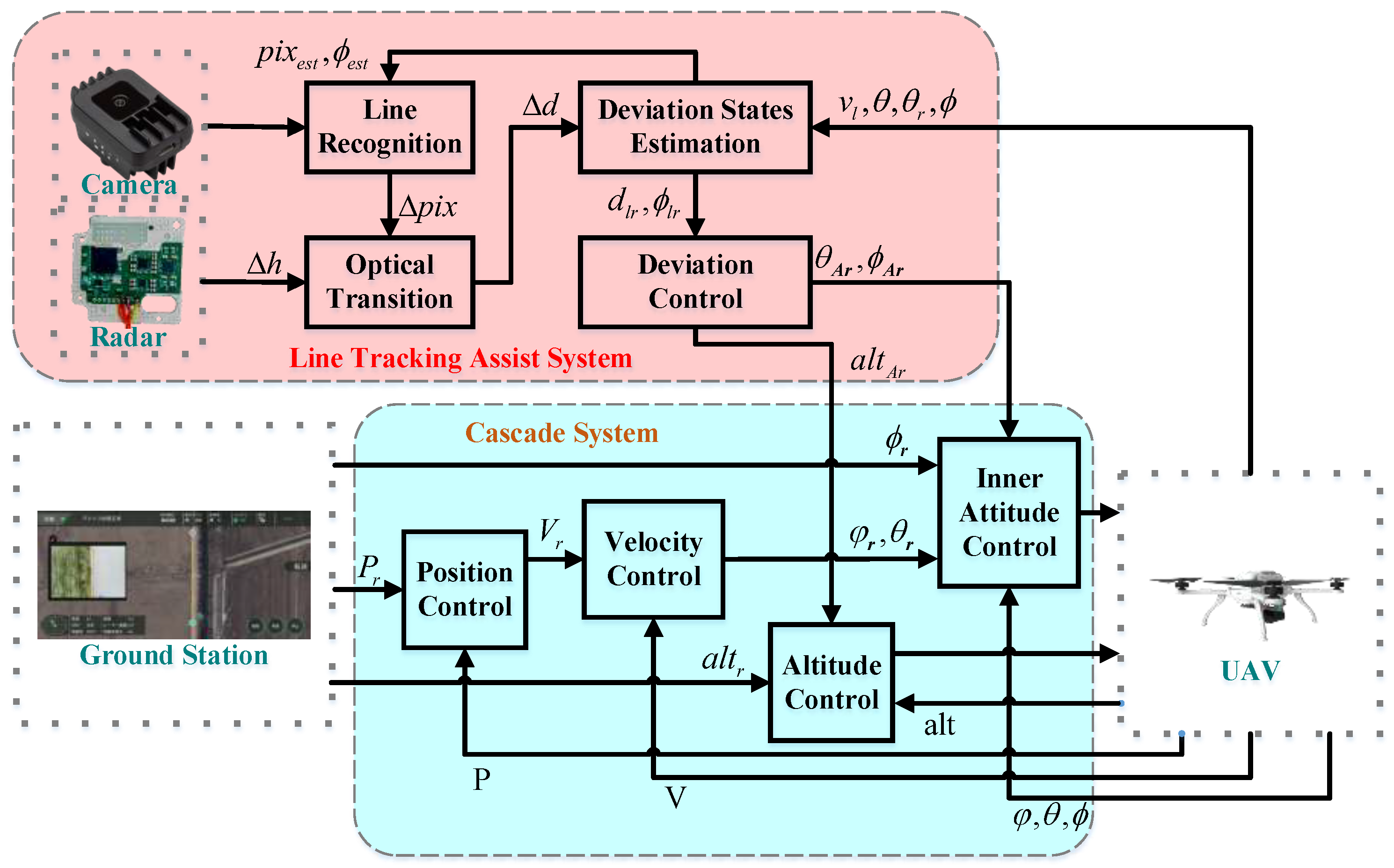
Considering the above points, this work addresses the design of a deviation control scheme for line inspection based on the waypoint mission. The method integrates data from cameras, radars, and GNSS sensors. It is important to note that the proposed scheme operates independently of the standard cascade control system in the drone control system. The overall structure of the proposed method is depicted in Figure 1.
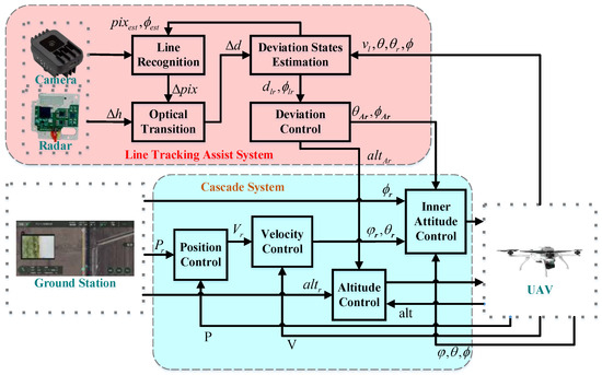
Figure 1.
The overall structure of the LTAS: Guided by waypoints from the ground station, which provide absolute position and heading angle information, the drone employs radar and camera systems to gather relative altitude, position, and heading angle data with the transmission line. The MobileNetV3 algorithm is utilized to recognize the transmission line. Subsequently, these data are used to refine the cascaded control of the UAV, aligning it more accurately with real-world conditions.
During inspection, drones fly above the transmission lines and utilize cameras to capture information. Line recognition, however, faces challenges due to interference from the complex ground environment, and the imaging characteristics of the transmission line can vary under different lighting conditions. Ensuring the stability of traditional line recognition schemes using fixed parameters for extracting transmission lines becomes difficult. An improved deep learning method is proposed to address this challenge. The transmission line’s position is also estimated by considering the drone’s lateral velocity. The estimated results are then used in the line recognition section to assist in selecting the transmission lines.
The LTAS is employed as an auxiliary system independent of the UAV primary control system, facilitating stable and precise control of the UAV directly above power transmission lines, and visual information is utilized within a visual serving approach in the control system. The inputs to the line assistance system include images captured by the camera , the relative height between the UAV and the power lines obtained from radar measurements, the UAV’s roll angle (neglecting this if the camera is fixed at the bottom of the aircraft and maintained level through the use of a gimbal), the UAV’s heading angle , the roll angle target value , and the lateral velocity of the UAV (computed by the UAV’s navigation algorithm, with the raw horizontal velocity input derived from the measurements of the GNSS sensor).
The output of the line assistance system consists of two components: one representing the additional target value for the roll angle and the other indicating the target value for the heading angle deviation . They are computed based on the lateral deviation distance and the heading angle deviation (between the UAV and the power lines) estimated by a deviation state observer.
The deviation state observer takes into consideration the lateral deviation distance between the UAV and the power lines obtained from visual data, the influence of the roll angle , the UAV’s heading angle , the roll angle target value , and the lateral velocity of the UAV. The observed results serve as input to the deviation controller and are utilized to estimate the probable position and orientation of the power lines in the image at the next time step. This information is then employed to allocate weights for line filtering during image recognition dynamically. This design offers two benefits: reducing misidentification and obtaining an accurate deviation state.
The lateral deviation distance is calculated using the pixel deviation obtained from visual data, the camera optical parameters, and the relative height between the UAV and the power lines measured by radar, employing the pinhole imaging principle.
The ground station provides the target heading angle , the altitude , and waypoints for the UAV. The UAV estimates the attitude using data from the three-axis angular velocity, the three-axis acceleration, and the three-axis magnetometer sensors. The resulting attitude angles (pitch angle , roll angle , heading angle ) serve as feedback for the inner-loop angular controller. The GNSS data undergo fusion through integrated navigation, yielding the position in the NED coordinate system. The latitude and longitude coordinate P serves as feedback for the position controller, the altitude as feedback for the altitude controller, and the horizontal velocity (obtained through coordinate transformation for the lateral UAV velocity in the body coordinates) as feedback for the velocity controller.
The three deviation control values output by the LTAS will act on the inner attitude controller (roll angle target value = cascade controller roll angle target value + LTAS correction controller roll angle output ; the heading angle target value = cascade controller heading angle target value + LTAS correction controller heading angle output ), and the altitude controller (altitude target value = integrated navigation feedback altitude + UAV set distance from power line height − radar height data ), respectively.
With the assistance of the LTAS, the drone can fly close to the transmission line without the need for expensive high-precision sensors, all while collecting detailed information. This scheme presents a novel and practical reference solution for TLI using drones.
3. Transmission Line Recognition
3.1. Line Recognition Description
GNSS coordinate drift poses a challenge due to factors like the ionospheric refraction error, the tropospheric refraction error, and the receiver clock error. Maintaining the drone’s relative position with the transmission line becomes difficult, especially in scenarios with known start and end points obtained from the ground station. In TLI, the camera is positioned below the drone, allowing the observation of lateral deviation between the drone and the transmission line through captured images. A radar sensor measures the relative vertical distance between the transmission line and the drone, while the horizontal deviation distance is calculated using images from the camera.
The obtained deviation distance enables the drone to perceive its deviation from the transmission line. Image processing aids the drone in predicting the position and angle of the transmission line in the image at the next moment. This allows for a more accurate selection of the line from the multiple lines detected in the image.
The line recognition system comprises a camera, a microcomputer, and a flight control system. The camera serves a dual purpose: capturing raw images of the transmission line and generating a binarized image corresponding to the raw image. Both sets of images are then transferred to the microcomputer.
The raw images are directly stored on the microcomputer, while the binarized image undergoes further processing through the Hough transform. This process extracts the position and heading deviation about the recognized transmission lines in the images. The microcomputer then matches the recognition results with the estimated results from the autopilot. The resulting transmission line is marked in the images with red stripes, facilitating viewing at the ground station. An overview of the entire process is illustrated in Figure 2.
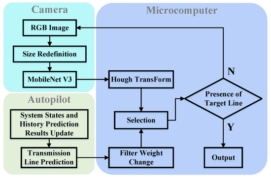
Figure 2.
The diagram depicts the structural framework of the line recognition system: Historical prediction outcomes encompass positional deviation and heading deviation computed by the microcomputer in the preceding moment. The microcomputer aligns the recognition results with the estimations derived from the autopilot to discern the most probable position of the transmission line.
3.2. Image Segmentation Based on Canny Edge Detection
The old scheme employs traditional edge detection for transmission line recognition in this program. In the given application scenario, Raspberry Pi is utilized as the image processing unit, necessitating consideration of its computational limitations. The preprocessing stage involves three primary steps: grayscale conversion, contrast enhancement, and denoising.
The raw RGB image is first grayscaled to alleviate the computational burden. The weighted average method (1) is deemed the most suitable choice among the classic and effective grayscale conversion methods. Grayscaling, calculated by adjusting the weights based on the characteristics of the target object, is expected to be more conducive to enabling the subsequent processes.
In the weighted average method (1), , , and represent the weights assigned to the R, G, and B channels, respectively, with the constraint that . Considering the different sensitivities of human vision to the primary colors, being highest for green and lowest for blue, the weight parameters should adhere to the condition .
While grayscaling the entire image reduces the computational burden on the processor, it may result in the loss of specific grayscale details. Therefore, contrast enhancement is deemed necessary. Given that the features of the detected transmission lines exhibit consistency, grayscale enhancement is achieved using the segmented linear transformation scheme (2).
In Equation (2), the three-stage segmented linear transform divides the gray range of the raw image into three segments: , , and , with corresponding transformations to , , and , resulting in .
When the transformed interval is larger than the original interval, it is labeled “stretching”; conversely, if the gap becomes smaller, it is marked “compression”. It is essential to note that various factors, such as the image sensors and the environmental conditions, can introduce noise to the image during image acquisition and transmission. Image filtering is necessary to address this issue. In this approach, the median filtering scheme is chosen for this task. While it effectively reduces noise, it is crucial to acknowledge that this filtering process may lead to the blurring of fine details, especially at the edges of the transmission line.
To accurately identify the features of transmission lines, the Canny operator is employed to detect changes in edges. This operator exhibits strong anti-interference characteristics and can retain edge information if it is the target. However, the extracted edge information often interferes, as pylons are built in highways, fields, and rivers. The collected images contain a lot of invalid backgrounds in addition to the transmission lines. After the edges of the image are extracted by the Canny operator, the edges of the interference backgrounds need to be removed, a process achieved by combining mask processing and morphological operations.
Mask processing is equivalent to superimposing an image with a transparent and opaque area on the image to be processed. The part of the raw images under the delicate area remains unchanged, while the opaque area is removed. In this way, practical regions of the images can be selected. Assuming that the image to be processed is , and the mask is , the expression formula of the final processed image is , as shown in Equation (3).
The color feature of the wire was chosen as the primary basis of the mask, and the color threshold of the RGB of the wire was adjusted according to the collected top view of the wire. Subsequently, this adjusted threshold was used for binarization of the raw color map of the transmission line.
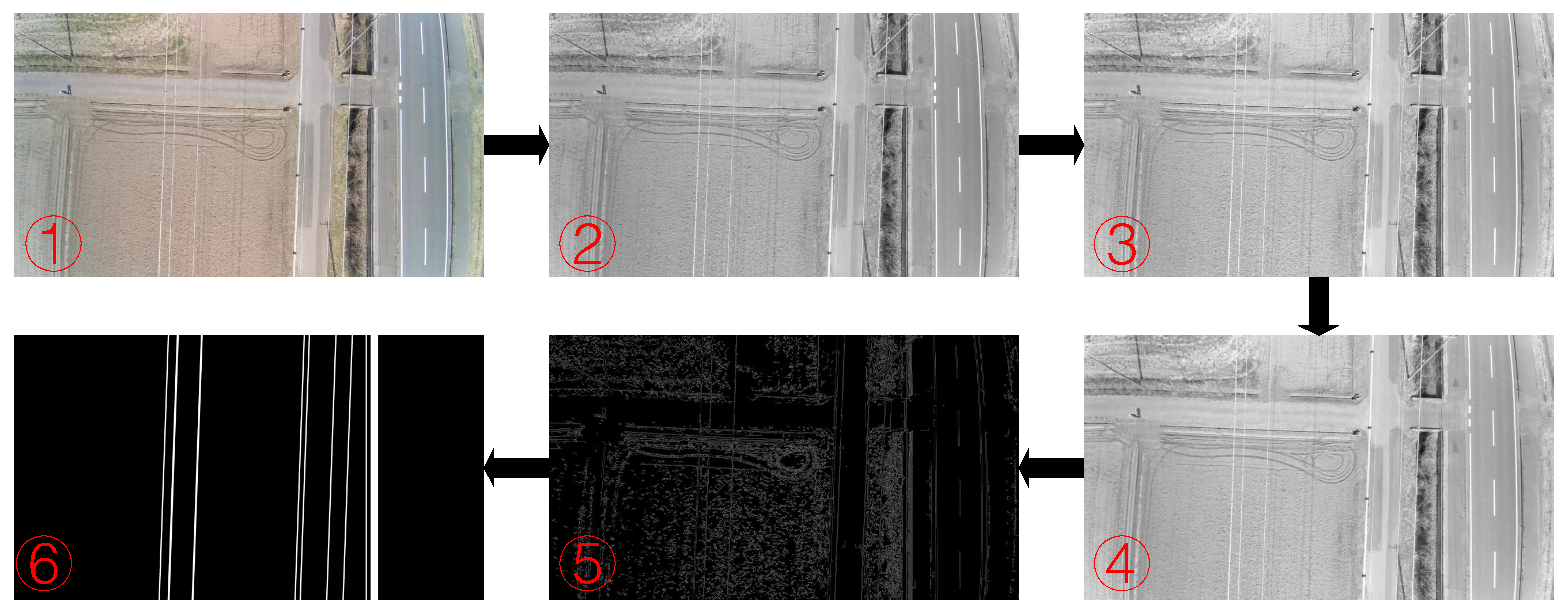
At this point, the preprocessing of the raw image has been completed. The entire processing process is depicted in Figure 3.

Figure 3.
Raw image preprocessing process: The first step involves capturing the raw RGB image from the camera. In the second step, grayscale conversion is applied to generate the grayscale image. The third step focuses on contrast enhancement to obtain more distinct edge information. Following that, the fourth step incorporates median filtering for noise reduction. The fifth step employs the Canny operator for edge detection. Lastly, the sixth step includes the Hough transform and mask processing.
3.3. Image Segmentation Based on MobileNetV3
As the backbone network, MobileNetV3 comprises multiple convolutional layers and extended convolutional layers, enabling it to extract rich feature information from the input image. Its lightweight architecture contributes to high computational and parametric efficiency, reducing the model’s complexity while maintaining accuracy. This characteristic makes it well suited for deployment in the drone ontology for line recognition.
Additionally, combining the context module, the channel-wise module, and the arm module enhances the efficiency and accuracy of the semantic segmentation tasks. This integrated approach results in more accurate segmentation outcomes while reducing the computational and parameter complexity concurrently.
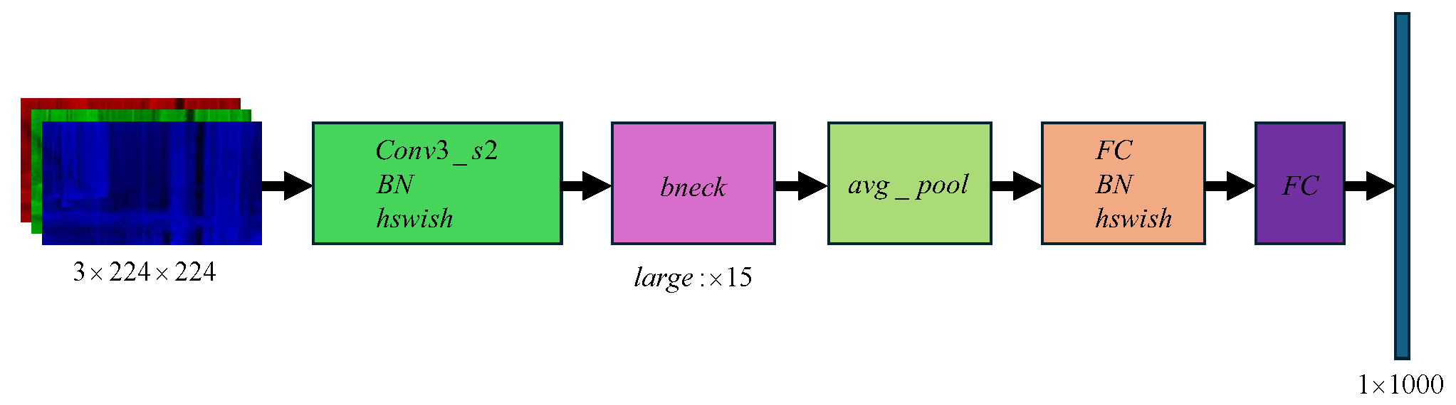
Figure 4 illustrates the network structure of MobileNetV3. Firstly, new nonlinear activation functions, h-swish and h-sigmoid, effectively reducing the computational costs, are introduced. Second, the block module is updated, and the squeeze-and-excitation (SE) module is incorporated, assigning a more considerable weight to specific channels to enhance accuracy. Third, the time-consuming layer structure is redesigned by eliminating convolutional kernels that contribute little to accuracy. The last stage is streamlined to improve the inference speed. Finally, leveraging the neural architecture search (NAS) for parameter optimization automates the search and selection of the best network structure, enhancing the performance and efficiency of the model.

Figure 4.
MobileNetV3 network structure.
3.4. Transmission Line Selection Strategy
After the Hough transform is finished, all the lines that satisfy the threshold in the image are extracted, containing single or multiple parallel lines and interference lines. In the actual inspection scenes, the ground line in the middle of numerous transmission lines is the primary target to be tracked. The remaining lines on both sides are still in the acquisition area. Therefore, extracting the desired line from the multiple recognition results must be considered.
After completing the Hough transform, all lines that meet the specified threshold in the image are extracted. These lines may include single or multiple parallel lines and interference lines. In practical inspection scenarios, the primary target for tracking is often the ground line in the middle of multiple transmission lines. The remaining lines on both sides are still within the acquisition area. Therefore, it becomes crucial to address the task of extracting the desired line from the multiple recognition results.
Two strategies are proposed to address this issue:
- Choose a forward straight line from the image’s center within the polar angle range of (−30, 30 degrees). Take note of the image dimensions as (, ). Ensure that the Y coordinate of the line’s midpoint falls within the specified threshold ().
- Record the pixel deviation and the polar angle of the previously recognized line in the preceding frame as and , respectively. Constrain the recognized results in the current frame within the ranges and , where and degrees serve as the specified limits.
After aligning the drone directly above the transmission line, ensuring the drone’s heading matches that of the line, Strategy 1 is applied. This strategy eliminates pairs of straight lines with angles significantly deviating from the drone’s heading and located far from the center of the screen. The selected pairs are then categorized into a set of straight lines. The optimal result is determined by choosing the group with the most significant consecutive lines within the collection. If the drone is not directly above the transmission line, the optimal output is determined by selecting the nearest straight line to the pixel point (, ).
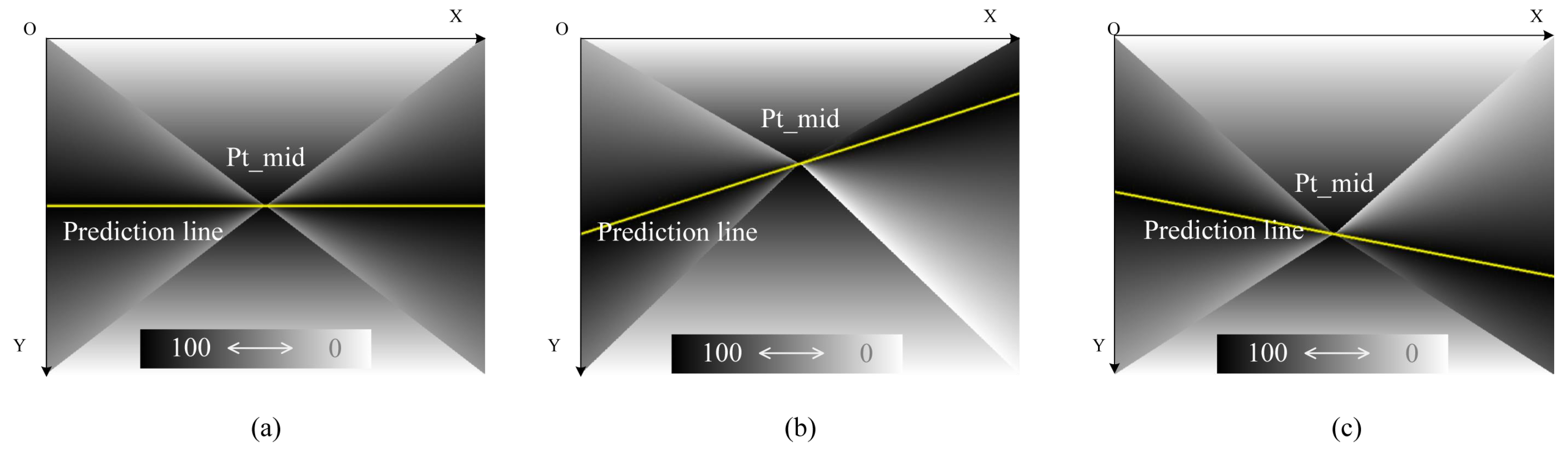
The drone initiates flight along the line after reaching the mission’s starting point and successfully recognizing the target transmission line. Simultaneously, Strategy 2 is activated. The corresponding weight changes are illustrated in Figure 5.
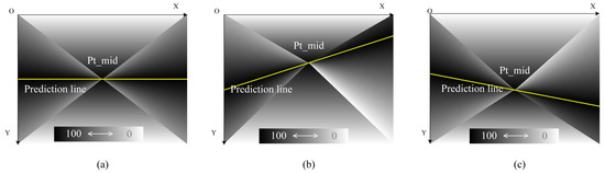
Figure 5.
Weight changes in different scenarios: The closer the color is to pure black, the higher the weight value. The yellow line represents the likely area for the transmission line to appear, as projected in the image. During inspection, (a) represents the optimal scenario for the weight distribution across the entire image. However, deviations such as the aircraft heading veering away from the transmission line direction and the aircraft body deviating from the position directly above the transmission line may lead to situations denoted as (b,c), and so forth.
In the grayscale diagram, weight is inversely proportional to the grayscale; smaller grayscale values indicate higher weights, and vice versa. The yellow line in Figure 5 signifies the straight line with the highest weight.
The weights are partitioned into two components: the angle and the position, with the angle taking precedence over the position. For instance, under Strategy 1, the weight assignment is illustrated in Figure 5a. The yellow line positioned in the center of the screen receives the highest weight. Any tilt or deviation from the screen’s center reduces its weight. The straight line with the maximum weight among the recognized lines is selected.
Figure 5b illustrates a scenario where the drone deviates to the right or tilts left. In this case, the weights favor positions closer to the x-axis on the screen. The polar angle from the previous moment increases, impacting the polar angle of the straight line on the screen. Similarly, Figure 5c depicts the opposite situation, with the yellow straight line representing the position with the highest weight.
4. Deviation Control System Design
4.1. Control System Structure
The proposed LTAS, as discussed in Section 2.2, utilizes the line recognition results as feedback to compute the auxiliary roll target. This target is integrated into the standard cascade control system, enhancing the drone’s lateral control to manage route deviations and external wind interference effectively.
For deviation control, is implemented using SMC. Additionally, a Kalman filter is employed to process the feedback information. The structure of this system is illustrated in Figure 6.
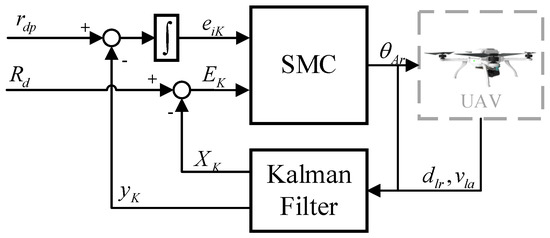
Figure 6.
Illustration of the deviation control system: Let , is designed to observe . The tracking target error and the state error are calculated with the corresponding state targets and the position target . is the auxiliary roll target calculated using an integral SMC method.
In Figure 6, the Kalman filter is employed to estimate the actual motion of the drone using inputs and . Considering the continuous and stable nature of , the filter proves effective in line recognition failure or misrecognition scenarios. The filter’s output includes and the process state . Additionally, is a component of the in-line selection, as introduced in Section 3.
Once the deviation feedbacks and are determined, the tracking target error and the state error are calculated with the corresponding state targets and the position target . Finally, an integral SMC method calculates the auxiliary roll target .
The subsequent sections will present a detailed discussion of the Kalman filter and the controller’s calculation process.
4.2. Deviation States Estimation
The outcome of line recognition, representing the real-time distance between the drone and the transmission line, is crucial for the efficacy of deviation control. However, environmental factors may cause this information to fail or be misrepresented, resulting in incorrect controller outputs and potentially impacting normal inspection operations. Consequently, the possibility of line recognition failure needs to be addressed.
A steady-state Kalman filter is employed to estimate the deviation distance to handle such situations, taking into account the lateral velocity of the drone.
Implementing the steady-state Kalman filter can be conceptualized as a linear system with multiple inputs. To realize this, knowledge of the system model is essential. Therefore, we first need to outline the dynamics of the deviation control system.
Given the context of inspection, where there is no significant attitude change (within 45 degrees) [29], and considering the system inputs and outputs, a second-order transfer function (4) proves sufficient for characterizing its properties [30,31,32].
The parameters , , and must be determined through fitting using actual flight data. This involves utilizing the target roll , the lateral velocity , and the line recognition result data. Once obtained, these parameters ensure that and meet the required criteria.
Let , where and . The deviation dynamics (5) can then be expressed in matrix form. Additionally, the integral of the lateral velocity is employed as the output.
with
Considering the Gaussian noise w on the input and the output measurement noise v, the discrete deviation system can be expressed as:
Here, , , and H correspond to the discretized A, B, and C. The design of the steady-state Kalman filter involves state and measurement update processes, as illustrated in (9) and (10).
where M represents the optimal innovation gain utilized to minimize the estimation errors under the noise covariances and . Finally, represents the estimated deviation state, and denotes the estimated deviation distance.
4.3. Integral SMC-Based Deviation Control Design
After completing the deviation distance estimation, a continuous and stable deviation feedback, , is obtained. This information is the basis for designing a deviation controller using an integral sliding mode control algorithm. The objective is to maintain the deviation distance at 0.3 m throughout the inspection, ensuring that the drone remains directly above the transmission line to capture information.
The controller design process assumes that the deviation state can be accurately estimated, i.e., and . Given the inspection task’s goal of keeping the drone stably above the line at all times ( and ), the tracking error is defined as . The integral of deviation is introduced to enhance the accuracy of deviation control as an extended state of the deviation dynamics, as depicted in (11).
Design the sliding mode surface , and its derivative form can be expressed as
Here, represents the parameters of the sliding surface corresponding to . Assuming that the deviation state converges to the surface and remains on it, . Consequently, the equivalent control can be calculated.
To mitigate the chattering phenomenon, one can replace the traditional sign function with a smoother function
where is a small positive constant for avoiding singular results. The switching control can be designed as
In (15), the switching gains A and B adjust the strength of the switching control. Finally, the output of the integral SMC-based deviation control is
5. Simulation and TLI Verification
5.1. Inspection Platform
To assess the effectiveness of the proposed scheme in practical applications, we developed a small quadcopter with a 247 mm wheelbase. The main sensors include an RGB camera and a GNSS receiver, as depicted in Figure 7.
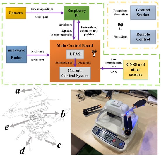
Figure 7.
Self-developed inspection platform and data/control flow among each component. The platform has a total weight of 0.484 kg and dimensions of 0.24 × 0.24 × 0.15 m. It mainly consists of the following components: GNSS receiver (a), main control board (b), RGB camera (c), mm-wave radar (d), and Raspberry Pi core board (e).
In the lower part of Figure 7, the specific distribution of each component is illustrated in Table 1.

Table 1.
Primary relevant sensors.
The GNSS receiver (a) provides the UAV with the raw position and velocity measurements (including the UAV lateral velocity to the LTAS).
The main control board (b) incorporates fundamental devices, such as the IMU, barometer, compass, and data logging module, enabling essential flight functionalities. It incorporates two STM32F4 chips, the primary chip handling communication and computation, while the secondary chip is responsible for data storage (flight logs and path recognition results recorded in the data logging module at 10 Hz).The proposed LTAS is developed in C within the IAR environment. It runs in conjunction with the flight control program (including the cascade control system) on the main chip of the control board.
The RGB camera (c) has the processing power of 4 TOPS and features onboard AI capabilities for image recognition.
The mm-wave radar PLK-LC2001l (d) detects the relative vertical distance between the drone and the transmission line. The measured distance is then used to convert the pixels and the actual altitude.
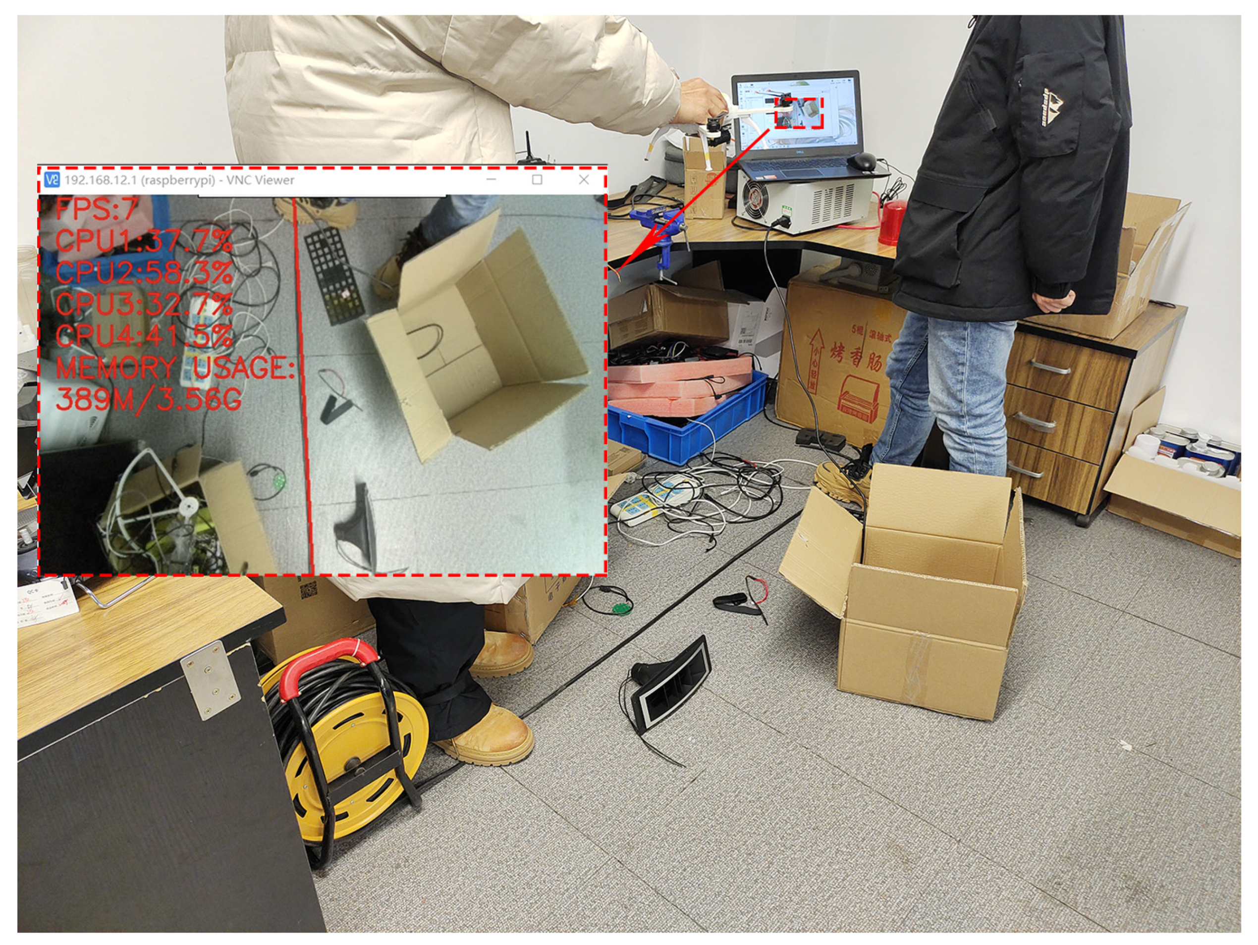
The Raspberry Pi (e) we selected has 4 GB of RAM and 32 GB of eMMC storage. To validate the feasibility of image processing, during experimentation, we displayed the Raspberry Pi’s processing frame rate, CPU utilization, and memory usage on the processed image output, as illustrated in Figure 8.

Figure 8.
Raspberry Pi operational status. In conditions of insufficient lighting and a cluttered environment, the Raspberry Pi outputs at a frame rate of approximately 7, with all four CPU cores utilizing 60% or less and the memory usage hovering around 400 MB.
In the upper section of Figure 7, the inter-device data/control flow is elucidated, with both the LTAS and the cascaded control system implemented on the main control board. Various sensors, such as the GNSS and the IMU (inertial measurement unit), communicate via the CAN protocol with the main control board. These real-time data streams to the main control board undergo integrated navigation processing, yielding real-time feedback for the UAV, including information such as the UAV position coordinates, the horizontal body lateral velocity, the roll angle, the heading angle, etc.
Communication between the ground station and the remote controller signals is established through the data link and the SBus link, facilitating remote communication with the main control board. The ground station transmits waypoint information to the main control board while the remote controller adjusts the UAV waypoints using the SBus interface. The camera communicates with the Raspberry Pi through a serial port, transmitting the processed line information and original images to the Raspberry Pi.
The millimeter-wave radar communicates with the main control board through a serial port on the Raspberry Pi, transferring raw deviation data to the LTAS system within the main control board. The deviation control input is integrated into the cascaded control system following deviation state estimation and control by the deviation controller. The cascaded control system, through a multi-level conversion of control inputs, ultimately assigns corresponding PWM signals to each motor, empowering the propellers to propel the UAV.
5.2. Line Recognition Verification
During power transmission line inspections, it becomes challenging to capture detailed information if the camera is positioned too far from the transmission lines. Even if the system can identify the straight lines representing the transmission cables, the significance of the inspection is compromised. It hinders detecting risks like bird nests or ice accumulation on the lines. Consequently, the system cannot implement effective mitigation measures.
The LARGE version of MobileNetV3 is selected; its specific parameter settings are detailed in Table 2.
Table 2.
Training parameters.
The dataset is augmented before training to enhance the segmentation effect, involving random rotation, random blurring, size adjustment, and image normalization. Random rotation aids in adapting to various wire orientations, and random blurring effectively addresses camera focusing issues, while size adjustment and normalization processing contribute to improved training efficiency.
During the model training process, a learning rate warm-up strategy is employed. Initially, the learning rate is set to a low value for a few epochs to facilitate a gradual convergence of the model towards stability. Subsequently, the predetermined learning rate is selected after ensuring the model has reached a relatively stable state. This approach accelerates the convergence of the model, leading to improved training effectiveness.
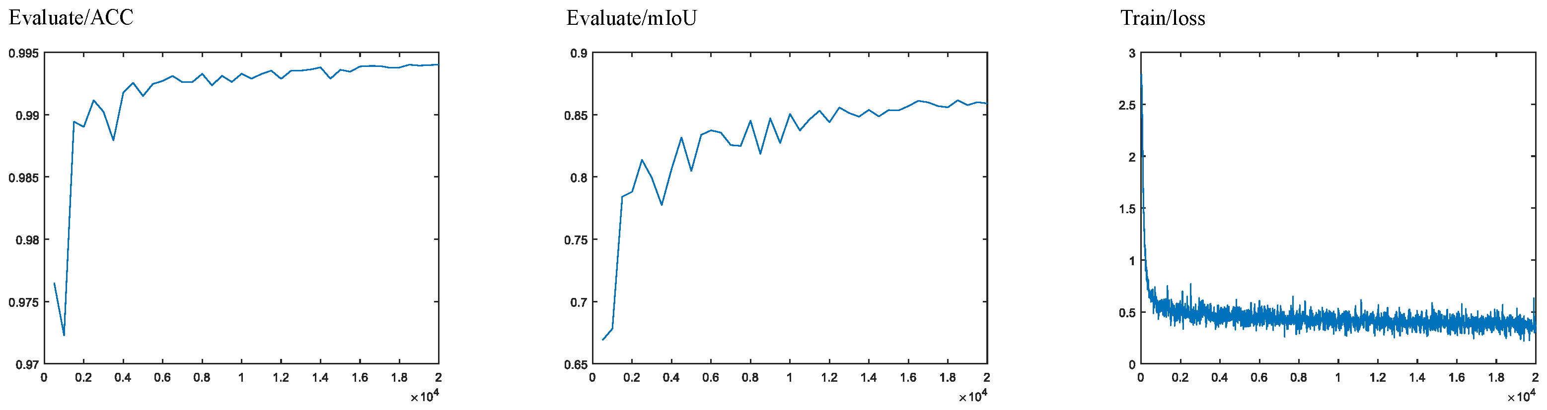
Stochastic gradient descent (SGD) is selected as the optimizer, and a hybrid loss function comprising the CrossEntropyLoss and the Lovasz Softmax loss is chosen. Throughout the training process, metrics such as the accuracy (ACC), the mean intersection over union (mIoU), and the loss values are monitored, as illustrated in Figure 9.
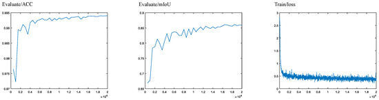
Figure 9.
ACC, mIoU, and loss values during the training process: ACC represents the ratio of pixels in the segmentation result that matches the actual situation to the total number of pixels. mIoU is the average of the ratio of intersection and concatenation between the segmentation result and the actual situation. The chosen loss function for the model is OhemCrossEntropyLoss, specifically selected to address the data distribution imbalance problem arising from a more significant number of background class samples than target class samples.
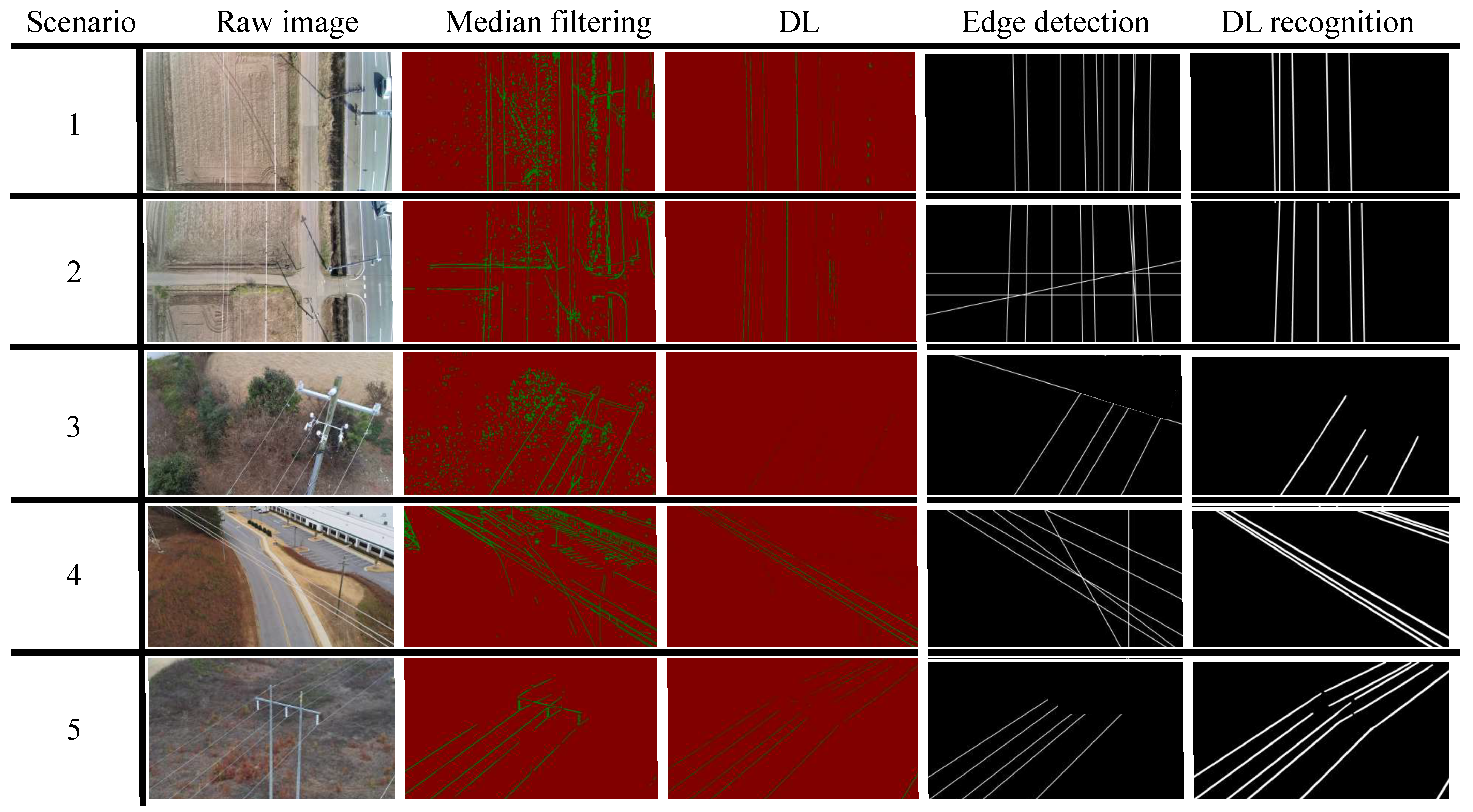
The parameters obtained from training are utilized for inference validation. Five scenarios were selected to assess the detection of transmission lines in different environments from varying perspectives. The results are presented in five columns, as shown in Figure 10. The first column displays the raw image, the second column showcases the result after processing the raw image with a median filter, and the third column illustrates the outcome of processing using the DL method.

Figure 10.
Line recognition process and results.
The final results of different methods are presented in the fourth and fifth columns. The fourth column displays the processing outcomes using the median filtered, the Hough transformed, and the masked. The fifth column reveals the results obtained through the proposed solution.
Examining the red background images in Figure 10, it is evident that utilizing the DL method for wire extraction offers undeniable advantages, effectively excluding interference in the background compared to median filtering. The black background reveals the final wire extraction results. For scenarios 1, 2, 3, and 4, the proposed scheme exhibits a more vital ability to filter out interference, as background interference has minimal impact on the method. Even for scenario 5, where the transmission line is nearly integrated into the background, the proposed scheme can still accurately extract the target wire segments.
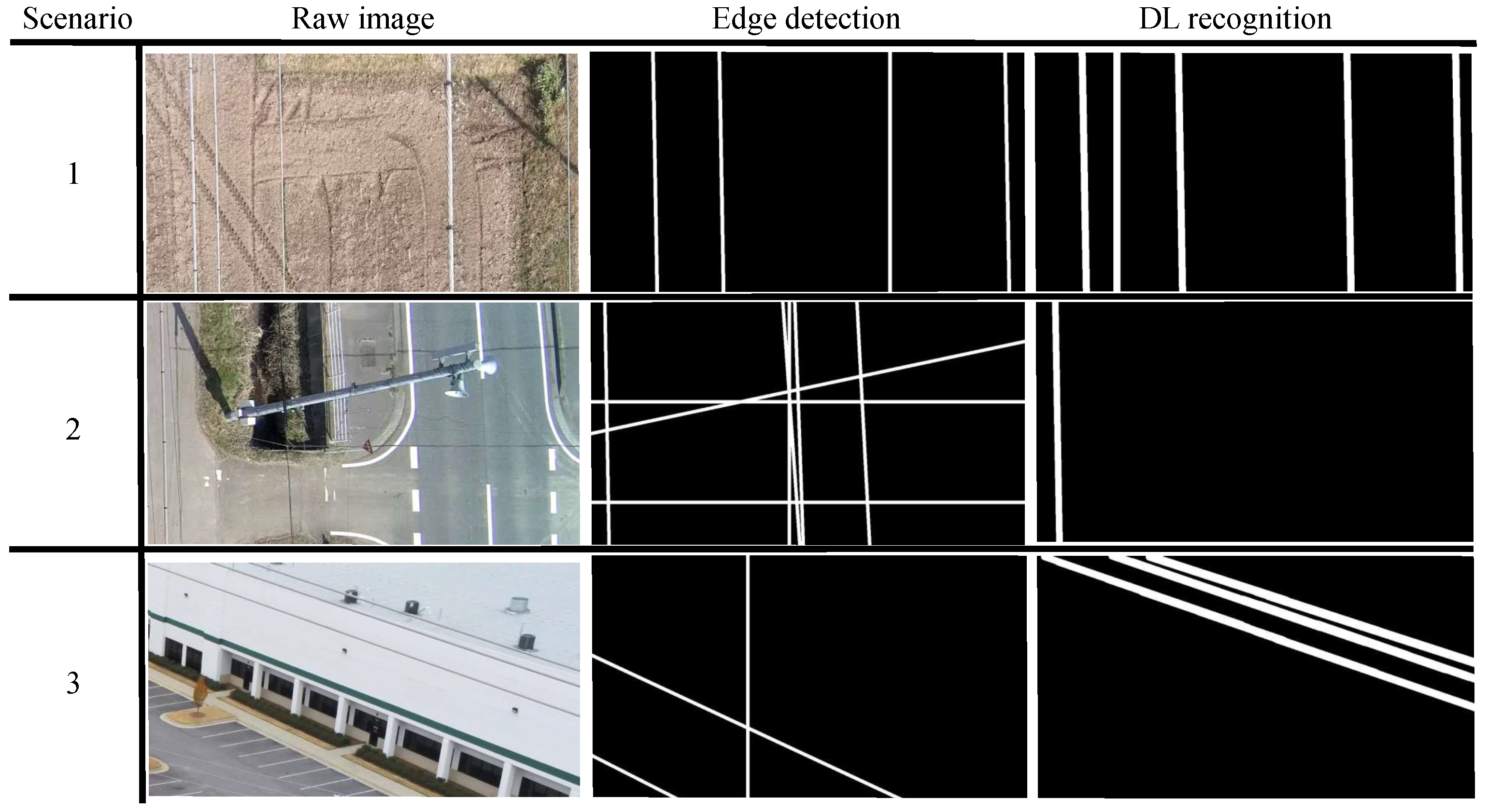
In Figure 11, a closer examination of scenarios 1, 2, and 4 from Figure 10 is presented, focusing on the recognition details. Scenario 1 in Figure 11 showcases the superior accuracy of the DL scheme compared to the edge detection methods. Scenario 2 highlights the potential issue with edge detection, where numerous straight lines unrelated to the transmission line are recognized, a challenge effectively addressed by the new scheme. Scenario 3 contrasts the limitations of the old method, which may identify the edge features of a house while overlooking the presence of the transmission line, in contrast to the new scheme’s accurate identification of the target.
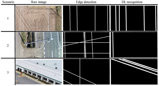
Figure 11.
Enlarged detail of line recognition process and results.
Hence, the proposed line recognition method recognizes transmission lines and demonstrates superior anti-interference capabilities against disturbances such as road marking lines.
5.3. Deviation Controller Verification
After completing the line recognition test in a static environment, further validation of the deviation control in the LTAS is essential in a dynamic environment before the actual inspection task. The process involves acquiring the lateral motion dynamics of the drone and designing the estimator (8) and controller (16).
Referring to 5, where and are the inputs and outputs, respectively, the lateral velocities are obtained by allowing the drone to operate freely in an open outdoor environment. The required states and are recorded at 50 Hz, consistent with the control frequency.
Utilizing the Ident toolbox in MATLAB, a fitting operation is performed on the recorded data to obtain the dynamics. Subsequently, the estimator and controller can be designed. For the designed inspection platform, the relevant parameters in the deviation control are listed in Table 3.
Table 3.
Parameters in deviation control.
For safety considerations, a 10-kilovolt transmission line environment with a lower height is chosen to verify the deviation control, as depicted in Figure 12. The inspection process aligns with previous work [27]: The drone autonomously takes off and elevates above the tower. Subsequently, the pilot operates the drone to maintain a position directly above the transmission line at the task’s starting point. The inspection flights commence, and the proposed LTAS is activated simultaneously. The entire experiment is conducted under the supervision of electric utility personnel.
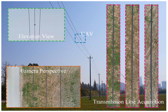
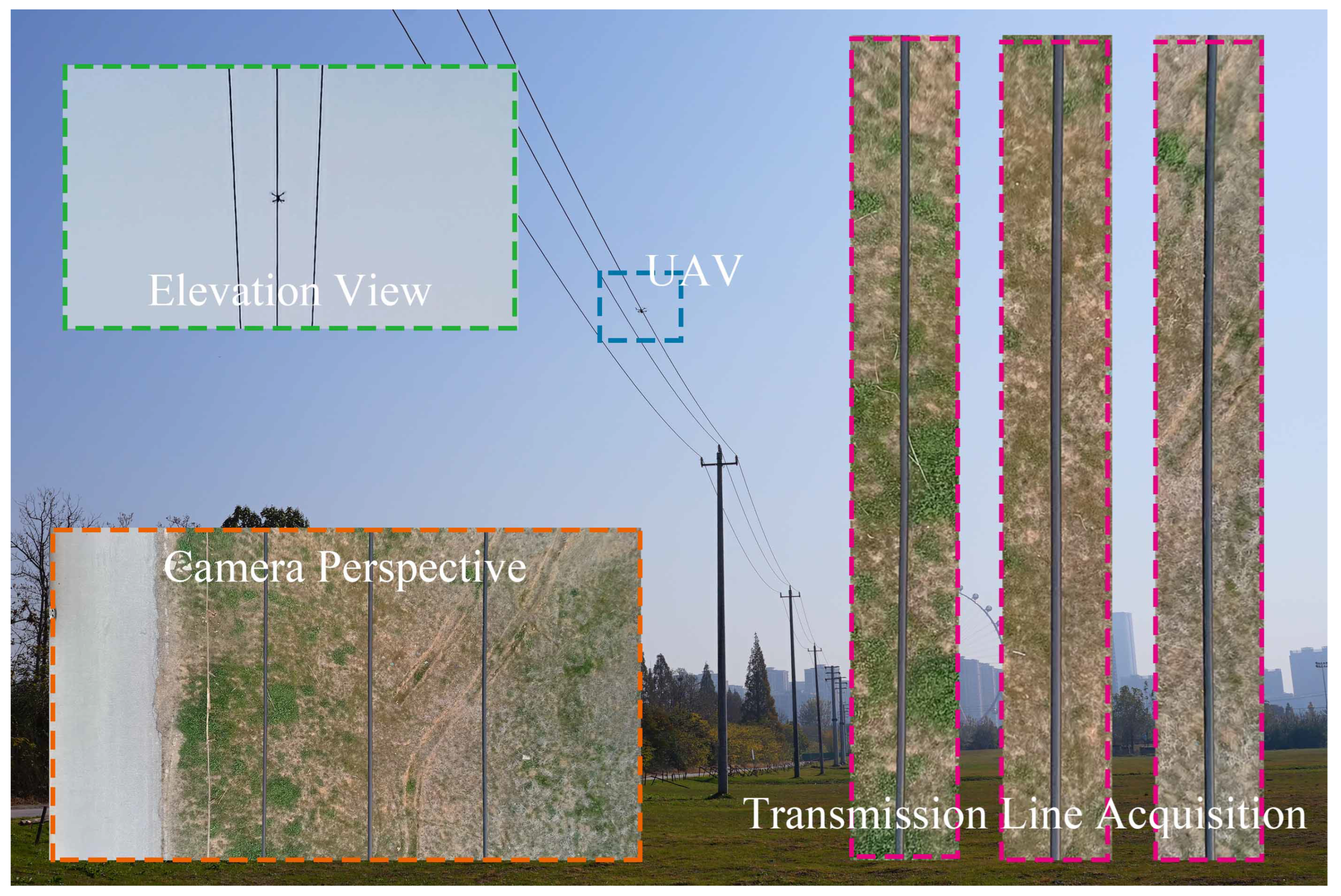
Figure 12.
Environment for deviation control validation. The UAV within the central blue frame is engaged in line inspection. The top-left corner displays the perspective captured from beneath the power line, while the bottom-left corner features a high-definition image recorded by the camera. The three images on the right depict magnified views from the camera’s perspective.
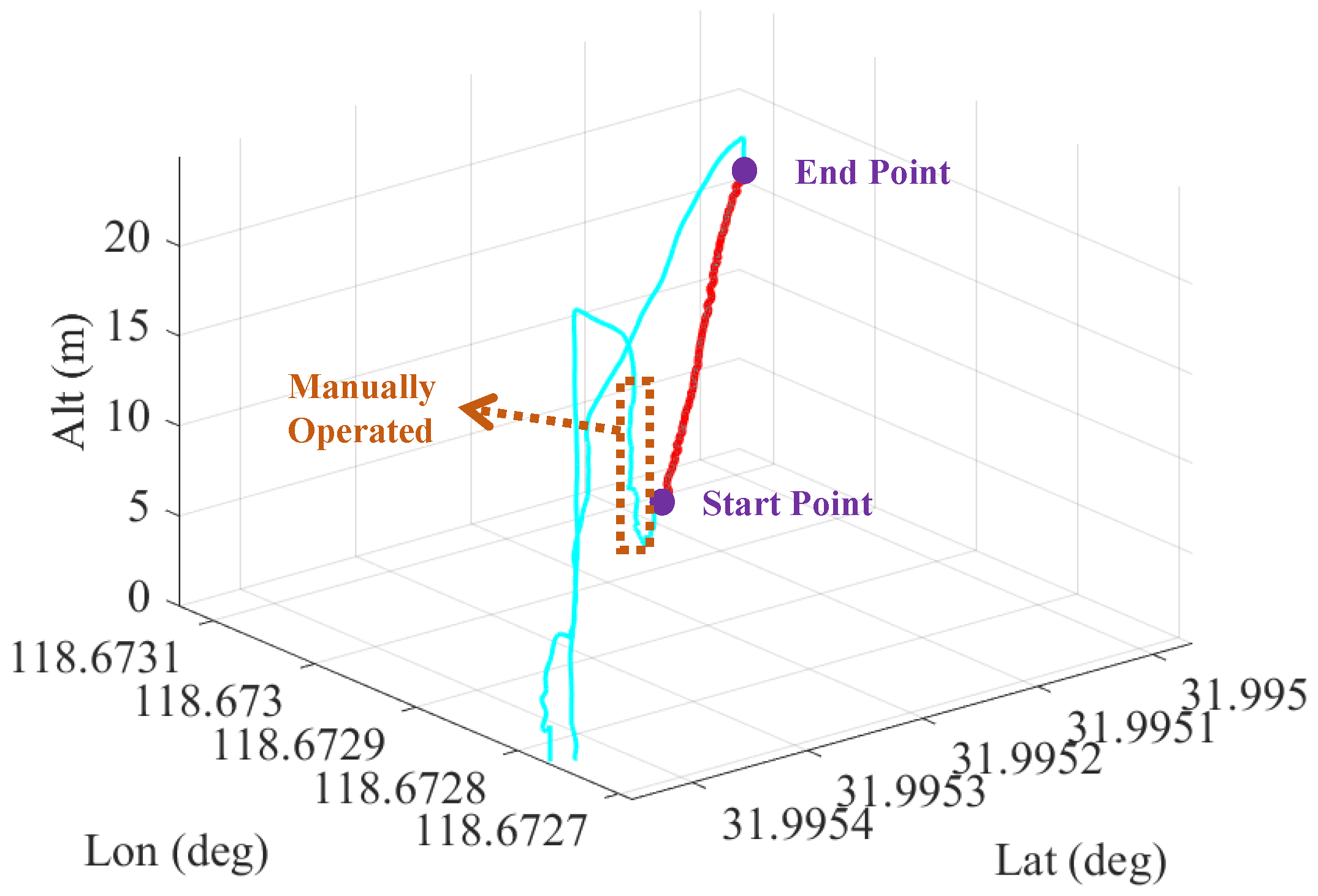
The drone’s flight trajectory is illustrated in Figure 13, with the effect of the LTAS highlighted by a red curve. Throughout this process, the estimator’s estimate of the lateral state is depicted in Figure 14. The pilot initially maneuvers the drone to the starting position. Subsequently, after reaching the endpoint, the drone returns to its take-off position.

Figure 13.
Flight trajectory during verification. This figure illustrates the flight trajectory recorded by the UAV, depicted in cyan, with the red segments indicating the active state of the LTAS.

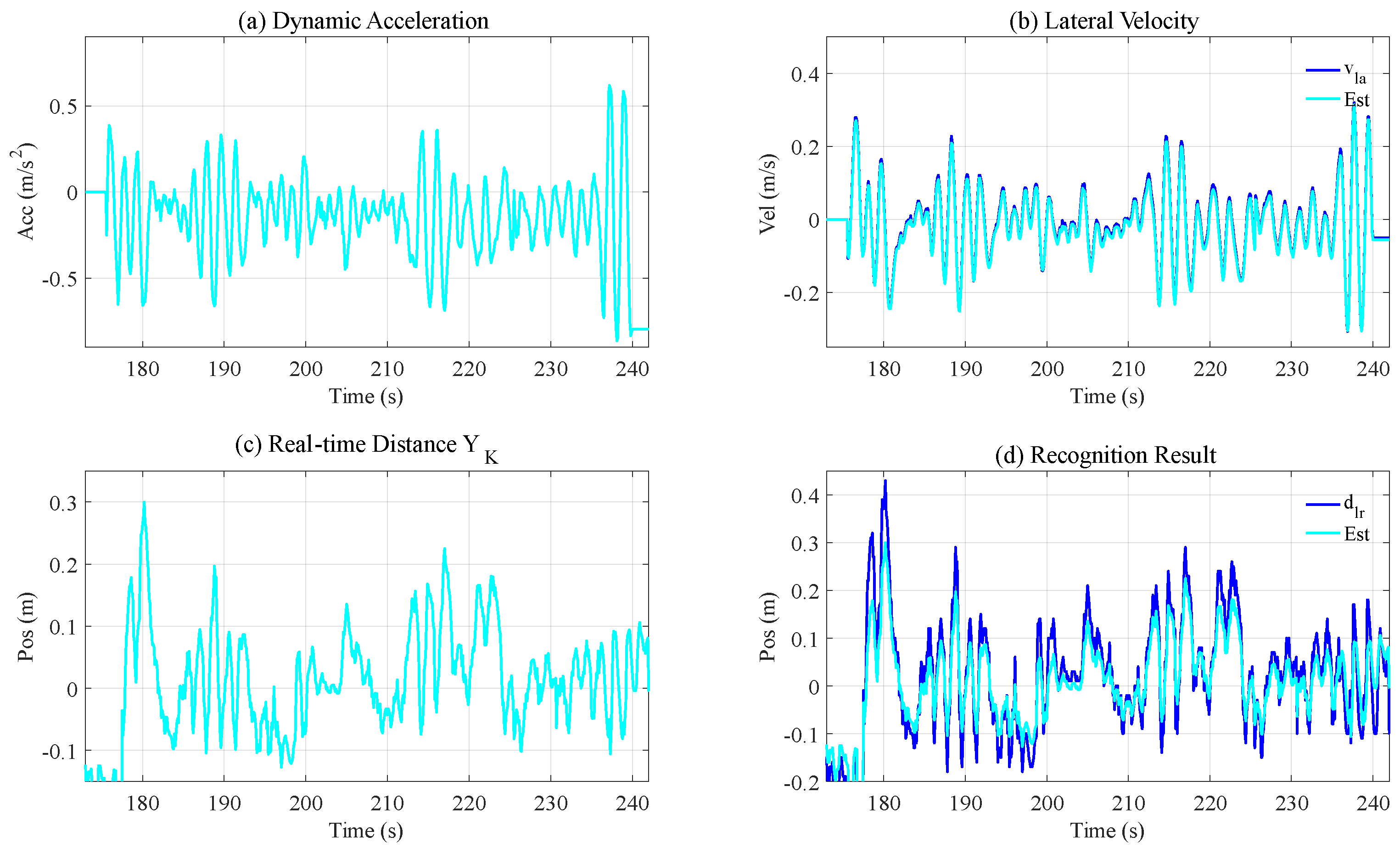
Figure 14.
State estimation during verification.
Figure 14 displays the estimation of the lateral state throughout the inspection process, encompassing the dynamic acceleration, the velocity, the real-time position, and the position with delay (line recognition result). Specifically, Figure 14b,d present the estimation of the lateral velocity and recognition results, respectively, allowing for a comparison with the actual measurement for verification. In Figure 14b, it is evident that the estimated velocity closely aligns with the actual measurement result . The position estimation results in Figure 14d align with the actual situation, effectively mitigating the influence of noise on the measurement results. Consequently, the implemented Kalman filter realistically responds to the lateral dynamics, and the estimated real-time position deviation can be further utilized for line selection in line recognition.
If the effective field of view is defined as the short edge from the center of the power line to the image edge, multiplied by 2, divided by the total image width, the value during normal operation should be no less than 30%, and during stable operation, it should be no less than 70%. Based on the selected camera’s horizontal field of view (68°), the inspection height (2 m), and the intended allowable free roll angle (15°), considering the deviation distance of the unmanned aerial vehicle from the power line, the normal working range should be within ±0.48 m, and the stable working range should be within ±0.21 m.
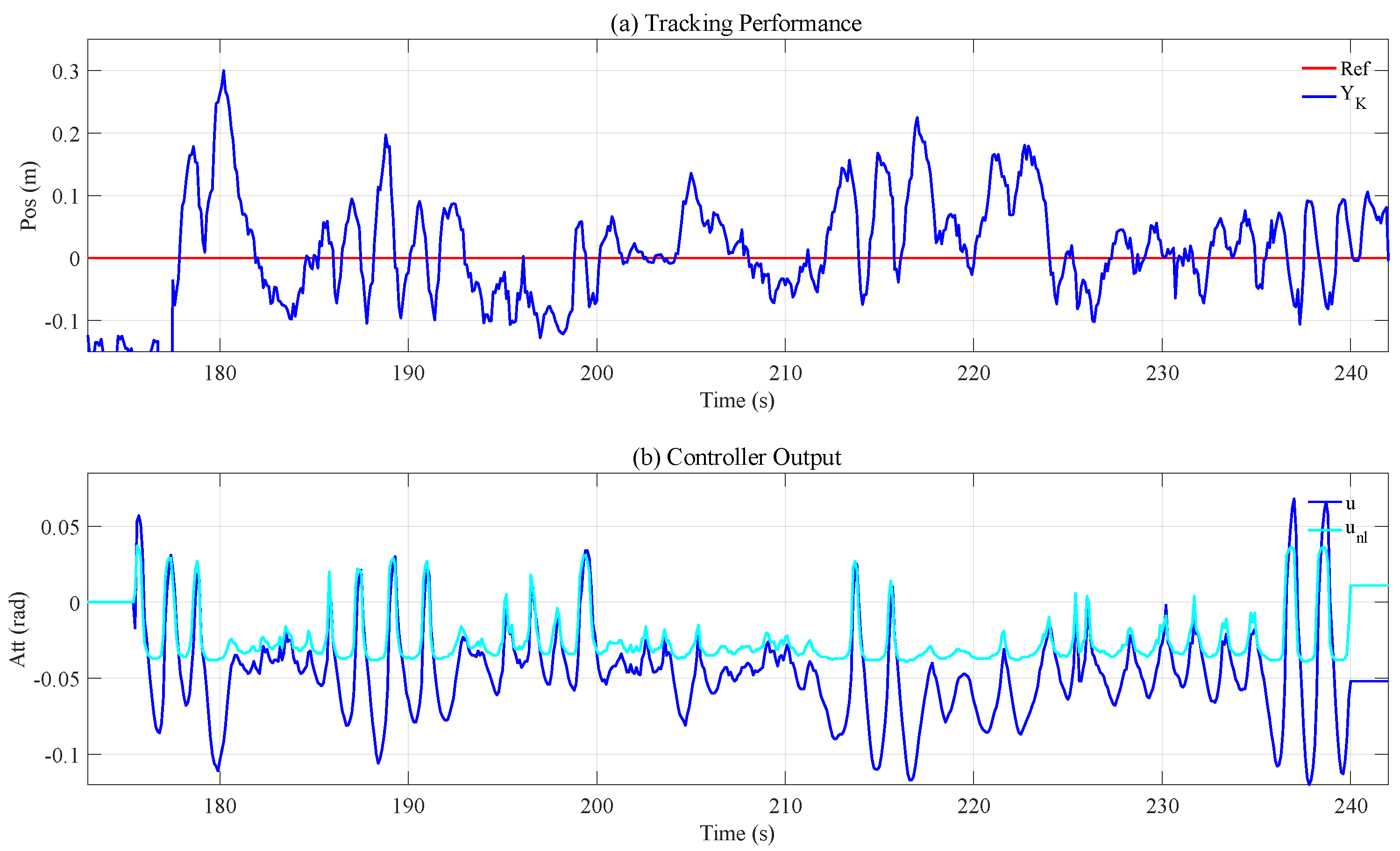
Using integral SMC, the drone maintains a consistent position directly above the transmission line with a target deviation of 0.1 m during flight. The tracking effect of the drone is illustrated in Figure 15.
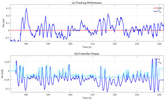
Figure 15.
Deviation control performance.
Figure 15a illustrates the deviation distances observed during the tracking process. It is evident that the distance between the UAV and the transmission line consistently remains within 0.2 m, ensuring continuous visibility of the entire transmission line for the camera. The outcomes of the controller computations are presented in Figure 15b, where the blue segment represents the total output, and the light blue color designates the calculated nonlinear component. This validation affirms that the designed integral sliding mode control (ISMC) maintains the UAV directly above the transmission line. Consequently, it can be inferred that the proposed LTAS enhances the UAV’s performance in inspection tasks.
5.4. Verification in TLI
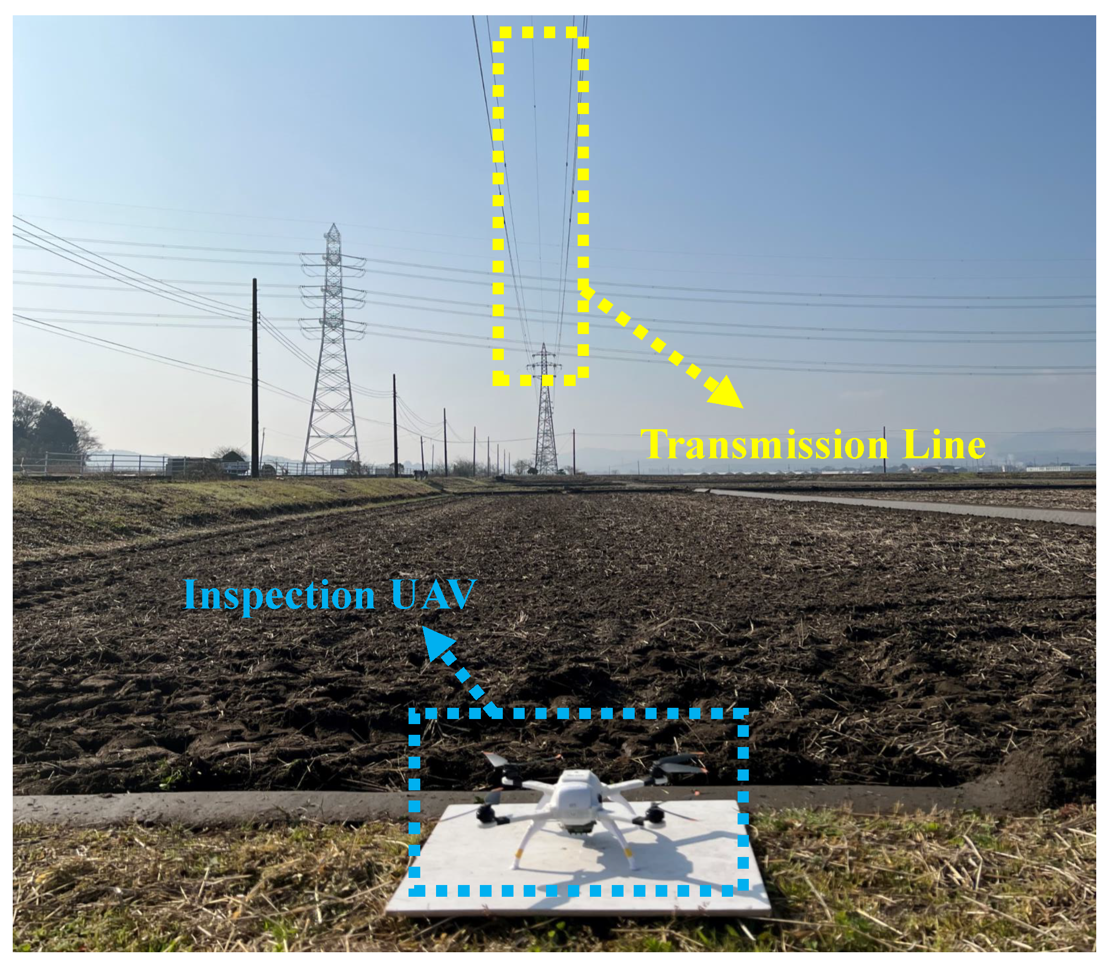
The inspection flight validation occurred near a pole tower in the Tomitsu Prefecture, Japan, depicted in Figure 16. The tower’s height is 41 m, and the ground line connecting the electricity pylon is the inspection target. Throughout the validation process, the total length of the transmission line under inspection is 137 m, with a geographic direction of 3 degrees. Notably, in this wild and open environment, the ground wind reaches a maximum of 4.6 m/s, presenting actual interference to the drone during inspection. Importantly, the entire validation process was conducted safely under the supervision of power practitioners.
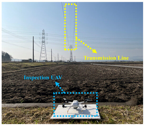
Figure 16.
Self-developed inspection platform.
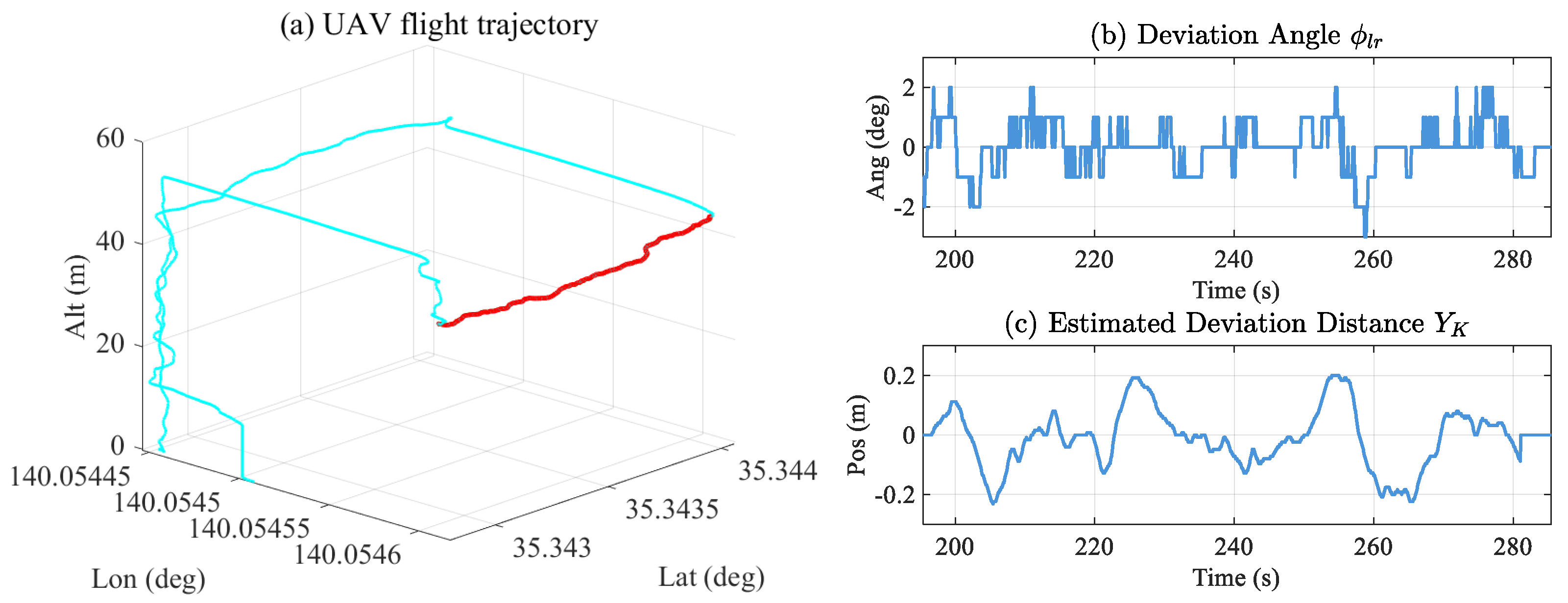
The inspection process mirrors the procedure outlined in Section 5.3. Following the pilot’s operation to position the drone directly above the transmission line, line recognition and deviation control mechanisms come into play, aiding in the precise execution of TLI. The drone’s recorded flight trajectory and the recognized deviations are presented in Figure 17.
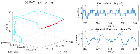
Figure 17.
Results of TLI: (a) illustrates the flight trajectory recorded by the UAV, depicted in cyan, with the red segments indicating the active state of the LTAS. In (b,c), the angle and distance deviations of the drone from the transmission line are presented, providing insights into the accuracy and effectiveness of the LTAS during the TLI process.
In Figure 17, the drone’s flight trajectory is depicted in Figure 17a, with the blue curves representing the drone’s flight directly above the transmission line and after the inspection is completed. The red segment illustrates the trajectory during the inspection above the transmission line. Throughout the inspection process, the angle and position deviations between the drone and the transmission line are recorded as in Figure 17b and Figure 17c, respectively. The recorded results indicate that the deviation reaches a maximum of only 3 degrees and consistently stays within degrees from the transmission line throughout the process. Notably, between 254.2 and 261.4 s, a change in the drone’s heading angle occurred due to external interference, promptly corrected, as demonstrated in Figure 18. The corresponding time points and the deviation data for each image are detailed in Table 4.
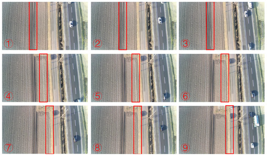
Figure 18.
Deviation correction during the inspection. The images are arranged chronologically, the first and second images depict the UAV heading in close alignment with the transmission line direction, slightly veering to the right. In the subsequent third to seventh images, the UAV exhibits deviations from the correct heading due to interference, followed by a process of correction. The eighth and ninth images demonstrate the UAV’s heading realignment with the transmission line direction once again.
Table 4.
Corrective performance under strong interference.
The real-time correction of the positional deviation between the drone and the transmission line is evident in Figure 17c. Although the performance is somewhat degraded compared to the inspection of the 10-kilovolt transmission line, primarily due to wind interference at higher altitudes, the recorded results demonstrate that the deviation is consistently maintained within the range of m throughout the inspection process. The mean value of the distance deviation is −0.01 m, ensuring that the tracked target transmission line remains consistently within the camera’s capture range.
The successful verification of the proposed line-tracking assistive system in a real high-voltage tower environment underscores its practical applicability to actual TLI work. Moreover, its adaptability to any inspection platform, leveraging low-cost sensors for proximity information acquisition of the transmission line, makes it a versatile and cost-effective solution.
6. Conclusions
This work focuses on the inspection tasks of transmission lines in UAV power inspections, utilizing RGB cameras, millimeter-wave radar, and GNSS receivers. We designed a novel line tracking assistance system consisting of three components: transmission line recognition, a deviation state estimator, and a deviation controller. To address the challenge of complex backgrounds in transmission line images, we employ the MobileNetV3 network for line recognition. Furthermore, leveraging millimeter-wave radar, we calculate the relative horizontal distance between the line and the UAV. Combining this information with navigation data from the GNSS receiver, the deviation state estimator provides more accurate deviation information. Lastly, based on the deviation information, the deviation controller, using a sliding mode algorithm, computes auxiliary attitude targets to ensure that the UAV consistently follows the transmission line during the inspection. The proposed solution is deployed on our in-house UAV platform and validated through flight tests in energized environments with 10-kilovolt and 110-kilovolt power towers. The experimental results confirm the effectiveness and practical feasibility of the proposed LTAS.
Additionally, the experimental outcomes reveal some limitations of the proposed solution. Variances in the along-line flight performance are observed in different working environments due to the simplistic linear model used in the deviation controller design, which does not account for external disturbances. Consequently, our future focus will be on improving the deviation controller to enhance the system’s versatility in diverse environments.
Author Contributions
Methodology, W.W.; Software, Z.S.; Validation, Z.S. and Z.Z. All authors have read and agreed to the published version of the manuscript.
Funding
This research received no external funding.
Data Availability Statement
Data are contained within the article.
Conflicts of Interest
The authors declare no conflict of interest.
References
- Katrasnik, J.; Pernus, F.; Likar, B. A survey of mobile robots for distribution TLI. IEEE Trans. Power Deliv. 2009, 25, 485–493. [Google Scholar] [CrossRef]
- Takaya, K.; Ohta, H.; Kroumov, V.; Shibayama, K.; Nakamura, M. Development of UAV system for autonomous power line inspection. In Proceedings of the 2019 23rd International Conference on System Theory, Control and Computing (ICSTCC), Sinaia, Romania, 9–11 October 2019; pp. 762–767. [Google Scholar]
- Savva, A.; Zacharia, A.; Makrigiorgis, R.; Anastasiou, A.; Kyrkou, C.; Kolios, P.; Panayiotou, C.; Theocharides, T. ICARUS: Automatic autonomous power infrastructure inspection with UAVs. In Proceedings of the 2021 International Conference on Unmanned Aircraft Systems (ICUAS), Athens, Greece, 15–18 June 2021; pp. 918–926. [Google Scholar]
- Luque-Vega, L.F.; Castillo-Toledo, B.; Loukianov, A.; Gonzalez-Jimenez, L.E. Power line inspection via an unmanned aerial system based on the quadrotor helicopter. In Proceedings of the MELECON 2014—2014 17th IEEE Mediterranean Electrotechnical Conference, Beirut, Lebanon, 13–16 April 2014; pp. 393–397. [Google Scholar]
- Gu, J.; Sun, R.; Chen, J. Improved Back-Stepping Control for Nonlinear Small UAV Systems with Transient Prescribed Performance Design. IEEE Access 2021, 9, 128786–128798. [Google Scholar] [CrossRef]
- Flores, G.; de Oca, A.M.; Flores, A. Robust Nonlinear Control for the Fully Actuated Hexa-Rotor: Theory and Experiments. IEEE Control. Syst. Lett. 2023, 7, 277–282. [Google Scholar] [CrossRef]
- Katrasnik, J.; Pernus, F.; Likar, B. New robot for power line inspection. In Proceedings of the 2008 IEEE Conference on Robotics, Automation and Mechatronics, Chengdu, China, 21–24 September 2008; pp. 1195–1200. [Google Scholar]
- Lopez, R.L.; Sanchez, M.J.B.; Jimenez, M.P.; Arrue, B.C.; Ollero, A. Autonomous uav system for cleaning insulators in power line inspection and maintenance. Sensors 2021, 21, 8488. [Google Scholar] [CrossRef] [PubMed]
- Jenssen, R.; Roverso, D. Automatic autonomous vision-based power line inspection: A review of current status and the potential role of deep learning. Int. J. Electr. Power Energy Syst. 2018, 99, 107–120. [Google Scholar]
- Yang, L.; Fan, J.; Liu, Y.; Li, E.; Peng, J.; Liang, Z. A review on state-of-the-art power line inspection techniques. IEEE Trans. Instrum. Meas. 2020, 69, 9350–9365. [Google Scholar] [CrossRef]
- He, T.; Zeng, Y.; Hu, Z. Research of multi-rotor UAVs detailed autonomous inspection technology of transmission lines based on route planning. IEEE Access 2019, 7, 114955–114965. [Google Scholar] [CrossRef]
- Fang, S.; Haiyang, C.; Sheng, L.; Xiaoyu, W. A framework of power pylon detection for UAV-based power line inspection. In Proceedings of the 2020 IEEE 5th Information Technology and Mechatronics Engineering Conference (ITOEC), Chongqing, China, 2–14 June 2020; pp. 350–357. [Google Scholar]
- Li, H.; Dong, Y.; Liu, Y.; Ai, J. Design and Implementation of UAVs for Bird’s Nest Inspection on Transmission Lines Based on Deep Learning. Drones 2022, 6, 252. [Google Scholar] [CrossRef]
- Yang, T.W.; Yin, H.; Ruan, Q.Q.; Han, J.D.; Qi, J.T.; Yong, Q.; Wang, Z.T.; Sun, Z.Q. Overhead power line detection from UAV video images. In Proceedings of the 2012 19th International Conference on Mechatronics and Machine Vision in Practice (M2VIP), Auckland, New Zealand, 28–30 November 2012; pp. 74–79. [Google Scholar]
- Zormpas, A.; Moirogiorgou, K.; Kalaitzakis, K.; Plokamakis, G.A.; Partsinevelos, P.; Giakos, G.; Zervakis, M. Power transmission lines inspection using properly equipped unmanned aerial vehicle (UAV). In Proceedings of the 2018 IEEE International Conference on Imaging Systems and Techniques (IST), Krakow, Poland, 16–18 October 2018; pp. 1–5. [Google Scholar]
- Li, Z.; Liu, Y.; Hayward, R.; Zhang, J.; Cai, J. Knowledge-based power line detection for UAV surveillance and inspection systems. In Proceedings of the 2008 23rd International Conference Image and Vision Computing New Zealand, Christchurch, New Zealand, 26–28 November 2008; pp. 1–6. [Google Scholar]
- Tian, F.; Wang, Y.; Zhu, L. Power line recognition and tracking method for UAVs inspection. In Proceedings of the 2015 IEEE International Conference on Information and Automation, Lijiang, China, 8–10 August 2015; pp. 2136–2141. [Google Scholar]
- Zhang, H.; Yang, W.; Yu, H.; Zhang, H.; Xia, G.S. Detecting power lines in UAV images with convolutional features and structured constraints. Remote Sens. 2019, 11, 1342. [Google Scholar] [CrossRef]
- Zhang, J.; Liu, L.; Wang, B.; Chen, X.; Wang, Q.; Zheng, T. High speed automatic power line detection and tracking for a UAV-based inspection. In Proceedings of the 2012 International Conference on Industrial Control and Electronics Engineering, Xi’an, China, 23–25 August 2012; pp. 266–269. [Google Scholar]
- Dietsche, A.; Cioffi, G.; Hidalgo-Carrió, J.; Scaramuzza, D. Powerline tracking with event cameras. In Proceedings of the 2021 IEEE/RSJ International Conference on Intelligent Robots and Systems (IROS), Prague, Czech Republic, 27 September–1 October 2021. [Google Scholar]
- Kim, S.; Kim, D.; Jeong, S.; Ham, J.W.; Lee, J.K.; Oh, K.Y. Fault diagnosis of power transmission lines using a UAV-mounted smart inspection system. IEEE Access 2020, 8, 149999–150009. [Google Scholar] [CrossRef]
- Cerón, A.; Mondragón, I.; Prieto, F. Onboard visual-based navigation system for power line following with UAV. Int. J. Adv. Robot. Syst. 2018, 15, 1729881418763452. [Google Scholar] [CrossRef]
- Deng, C.; Liu, J.Y.; Liu, Y.B.; Tan, Y.Y. Real time autonomous transmission line following system for quadrotor helicopters. In Proceedings of the 2016 International Conference on Smart Grid and Clean Energy Technologies (ICSGCE), Chengdu, China, 19–22 October 2016; pp. 61–64. [Google Scholar]
- Mirallès, F.; Hamelin, P.; Lambert, G.; Lavoie, S.; Pouliot, N.; Montfrond, M.; Montambault, S. LineDrone Technology: Landing an unmanned aerial vehicle on a power line. In Proceedings of the 2018 IEEE International Conference on Robotics and Automation (ICRA), Brisbane, Australia, 21–25 May 2018; pp. 6545–6552. [Google Scholar]
- Schofield, O.B.; Iversen, N.; Ebeid, E. Autonomous power line detection and tracking system using UAVs. Microprocess. Microsystems 2022, 4, 104609. [Google Scholar] [CrossRef]
- Malle, N.H.; Nyboe, F.F.; Ebeid, E.S.M. Onboard Powerline Perception System for UAVs Using mmWave Radar and FPGA-Accelerated Vision. IEEE Access 2022, 10, 113543–113559. [Google Scholar] [CrossRef]
- Wang, Q.; Wang, W.; Li, Z.; Namiki, A.; Suzuki, S. Close-Range Transmission Line Inspection Method for Low-Cost UAV: Design and Implementation. Remote Sens. 2023, 15, 4841. [Google Scholar] [CrossRef]
- Zhou, G.; Yuan, J.; Yen, I.L.; Bastani, F. Robust real-time UAV based power line detection and tracking. In Proceedings of the IEEE International Conference on Image Processing (ICIP), Phoenix, AZ, USA, 25–28 September 2016; pp. 744–748. [Google Scholar]
- Abro, G.E.M.; Zulkifli, S.A.B.; Asirvadam, V.S.; Ali, Z.A. Model-free-based single-dimension fuzzy SMC design for underactuated quadrotor UAV. Actuators 2021, 10, 191. [Google Scholar] [CrossRef]
- Wang, W.; Ma, H.; Xia, M.; Weng, L.; Ye, X. Attitude and altitude controller design for quad-rotor type MAVs. Math. Probl. Eng. 2013, 2013, 587098. [Google Scholar] [CrossRef]
- Li, B.; Li, Q.; Zeng, Y.; Rong, Y.; Zhang, R. 3D trajectory optimization for energy-efficient UAV communication: A control design perspective. IEEE Trans. Wirel. Commun. 2021, 21, 4579–4593. [Google Scholar] [CrossRef]
- Wang, Q.; Wang, W.; Suzuki, S.; Namiki, A.; Liu, H.; Li, Z. Design and Implementation of UAV Velocity Controller Based on Reference Model Sliding Mode Control. Drones 2023, 7, 130. [Google Scholar] [CrossRef]
- NEO-M8 Series. Available online: https://www.u-blox.com/en/product/neo-m8-series (accessed on 5 January 2024).
- STM32F4 Series. Available online: https://www.st.com/en/microcontrollers-microprocessors/stm32f4-series.html (accessed on 5 January 2024).
- IAR. Available online: https://www.iar.com/ (accessed on 5 January 2024).
- OAK–1. 2020. Available online: https://shop.luxonis.com/collections/oak-cameras-1/products/oak-1-max (accessed on 5 January 2024).
- PLK–LC2001l. 2020. Available online: http://www.plcomp.com/Home/detail.html/3011 (accessed on 5 January 2024).
- Raspberry Pi Compute Module 4. Available online: https://www.raspberrypi.com/products/compute-module-4/?variant=raspberry-pi-cm4001000 (accessed on 5 January 2024).


Disclaimer/Publisher’s Note: The statements, opinions and data contained in all publications are solely those of the individual author(s) and contributor(s) and not of MDPI and/or the editor(s). MDPI and/or the editor(s) disclaim responsibility for any injury to people or property resulting from any ideas, methods, instructions or products referred to in the content. |
© 2024 by the authors. Licensee MDPI, Basel, Switzerland. This article is an open access article distributed under the terms and conditions of the Creative Commons Attribution (CC BY) license (https://creativecommons.org/licenses/by/4.0/).