HeightFormer: A Multilevel Interaction and Image-Adaptive Classification–Regression Network for Monocular Height Estimation with Aerial Images

Abstract

Height estimation has long been a pivotal topic within measurement and remote sensing disciplines, with monocular height estimation offering wide-ranging data sources and convenient deployment. This paper addresses the existing challenges in monocular height estimation methods, namely the difficulty in simultaneously achieving high-quality instance-level height and edge reconstruction, along with high computational complexity. This paper presents a comprehensive solution for monocular height estimation in remote sensing, termed HeightFormer, combining multilevel interactions and image-adaptive classification–regression. It features the Multilevel Interaction Backbone (MIB) and Image-adaptive Classification–regression Height Generator (ICG). MIB supplements the fixed sample grid in the CNN of the conventional backbone network with tokens of different interaction ranges. It is complemented by a pixel-, patch-, and feature map-level hierarchical interaction mechanism, designed to relay spatial geometry information across different scales and introducing a global receptive field to enhance the quality of instance-level height estimation. The ICG dynamically generates height partition for each image and reframes the traditional regression task, using a refinement from coarse to fine classification–regression that significantly mitigates the innate ill-posedness issue and drastically improves edge sharpness. Finally, the study conducts experimental validations on the Vaihingen and Potsdam datasets, with results demonstrating that our proposed method surpasses existing techniques.

1. Introduction

With the advancement of high-resolution sensors in the field of remote sensing [1,2], the horizontal pixel resolution (the horizontal distance represented by a single pixel) of the visible light band for ground observation from satellite/aerial platforms has reached the level of decimeters or even centimeters. This has made various downstream applications such as fine-grained urban 3D reconstruction [3], high-precision mapping [4], and MR scene interaction [5] incrementally achievable. Among these applications, the ground surface height value (Digital Surface Model, DSM) serves as a primary data support, and its acquisition methods have been a focal point of research [6].

Numerous studies on height estimation have been published, among which methods based on LiDAR demonstrate the highest measurement accuracy [7]. These techniques involve calculating the time difference between wave emission and reception to ascertain the distance to corresponding points, with further adjustments to generate height values. However, the high power consumption and costly equipment required for LiDAR significantly constrain its application in satellite/UAV scenarios. Another prevalent method is stereophotogrammetry, as developed by researchers like Nemmaou et al. [8], which utilizes prior knowledge of perspective differences from multiple images or multi-angles to fit height information. Furthermore, Hoja et al. and Xiaotian et al. [9,10] have employed multisensor fusion methods combining stereoscopic views with SAR interferometry, further enhancing the quality of the estimations. While stereophotogrammetry significantly reduces both power consumption and equipment costs compared to LiDAR, its high computational demands pose challenges for sensor-side deployment and real-time computation.

Recently, numerous monocular deep learning algorithms have been proposed that, when combined with AI-capable chips, can achieve a balance between computational power and cost (latency <100 ms, chip cost < USD 50, chip power consumption <3 W). Among these, convolutional neural network (CNNs) models, widely applied in the field of computer vision, have begun to be utilized in monocular height estimation [11]. CNNs excel in reconstructing details like edges and offer controllable computational complexity. However, as monocular height estimation is inherently an ill-posed problem [12], it demands more advanced information extraction. CNNs use a fixed receptive field for information extraction, making it challenging to interact with information at the level of the entire image. This limitation often leads to common issues such as instance-level height deviations (overall deviation in height prediction for individual, homogeneous land parcels) like Figure 1a, which restrict the large-scale application of monocular height estimation.

But the advent of transformers and their attention mechanisms [13], which capture long-distance feature dependencies, has significantly improved the inadequate whole-image information interaction common to CNN models. Transformers have been progressively applied in remote sensing tasks such as object detection [14] and semantic segmentation [15]. Among these developments, the Vision Transformer (ViT) [16] was an early adopter of the transformer approach in the visual domain, yet it encounters two primary issues. First, the high computational complexity and difficulty in model convergence: As shown in Figure 2a, ViT, by emulating the transformer’s approach used in natural language processing, constructs attention among all tokens (small segments of an image). Given that height prediction is a dense generation task requiring predictions for all pixel heights, this leads to an excessively high overall computational complexity and challenges in model convergence. Second, the original ViT’s edge reconstruction quality is mediocre. Due to the lack of inductive bias in the transformer’s attention mechanism, which is inherent in CNNs, although it achieves better average error metrics (REL) by reducing overall instance errors, it underperforms in edge reconstruction quality between instances compared to CNN models, resulting in edge blurring issues akin to those observed in Figure 1b.

In response to the high computational complexity and the edge blurring issue stemming from ViT’s lack of local modeling, this paper introduces a multiscale interactive adaptive classification–regression height estimation network (Heightformer). In the encoder stage, as shown in Figure 2b, we have developed a Multiscale Interactive Backbone Encoder (MIBE). This approach modifies the ViT encoder, which performs global attention at all layers, into a lightweight three-tier module: a convolutional backbone network for extracting pixel-level features (having the smallest information interaction range, primarily for extracting information from adjacent pixels), a local attention backbone network for extracting patch-level features (with a moderate range of information interaction, mainly interacting within 1/4 of the image scope), and a cross-channel attention fusion module at the tail of the encoder (for global information interaction across channel dimensions with the heterogeneous feature maps extracted by the two backbones). By segmenting the information interaction range, we optimized the information acquisition at each level with less than a third of the parameter amount of a standard ViT encoder, thereby enhancing the quality of edge reconstruction.

In the decoder stage, we propose an Image-adaptive Classification–Regression Height Generator (ICG), which significantly reduces the parameter optimization space of the decoder through a classification–regression mechanism [17]. This includes a branch for calculating adaptively classified height values for the current input image and another for computing the corresponding probability of height values. As depicted in Figure 3, adaptive height values are better suited to fit the data distribution of the current image, thereby improving edge reconstruction quality. Adabins [18] was among the first to adopt an image-adaptive strategy, but it introduced ViT only in the decoder stage, leading to limited acquisition of global features and poorer edge reconstruction quality. Sun et al. [19] used a single-layer transformer for predicting height values, which was entirely independent from the upsampling convolution process of the probability map branch. They also constructed cross-attention using a randomly initialized query with the encoder output, resulting in instability in height value generation and suboptimal reconstruction metrics. In contrast, our method entails constructing coupled height prediction and probability map generation layers. By incorporating the output of the probability branch into each height prediction layer and combining it with positional encoding embedding to build cross-attention, we ensure that the generated height values are compatible with the depth of the current image. This approach improves edge reconstruction quality while balancing model robustness and computational complexity.

Our contributions can be summarized as follows:

1. This paper addresses the challenges of high computational complexity and average edge reconstruction quality in existing ViT-based and adaptive classification–regression methods for monocular height estimation tasks. It proposes a novel remote sensing monocular height estimation method (Heightformer) utilizing multiscale interaction and image-adaptive classification–regression. This approach effectively balances instance reconstruction and edge reconstruction quality while maintaining manageable model complexity.

2. The proposed Multilevel Interaction Backbone Encoder (MIBE) is based on ResNet-18, Swin-Transformer-Tiny, and a cross-channel attention module. It achieves pixel-level, patch-level, and channel-level (global) feature extraction, significantly reducing the encoder size while facilitating multiscale interaction.

3. The proposed Image-adaptive Classification–Regression Height Generator (ICG) employs coupled reconstruction layers to generate depth-matched height values for different images, effectively mitigating the issue of edge blurring.

4. Experiments are conducted on the Vaihingen and Potsdam datasets, with comparison results indicating that HeightFormer outperforms current remote sensing and computer vision methods while achieving higher Rel metrics with a smaller number of parameters.

The rest of this paper is organized as follows. In Section 2, we briefly introduce the related work. Section 3 explains the details of the HeightFormer framework, and extensive experiments are presented in Section 4. Finally, Section 5 concludes this article.

2. Related Work

2.1. Overview

Height estimation is a key component of 3D scene understanding [20] and has long held a significant position in the domains of remote sensing and computer vision. Initial research predominantly focused on stereo or multi-view image matching. These methodologies [21] typically relied on geometric relationships for keypoint matching between two or more images, followed by using triangulation and camera pose data to compute depth information. Recently, with the advent of large-scale depth datasets [22], research focus has shifted. The current effort is centered on estimating distance information from monocular 2D images using supervised learning. Present monocular height estimation approaches can be generally categorized into three types [23,24,25,26]: methodologies based on handcrafted features, methodologies utilizing convolutional neural networks (CNN), and methodologies based on attention mechanisms. In general, due to the datasets containing various types of features, it is challenging to extract only manual features to fit the distribution of different datasets, and the effectiveness is generally moderate.

2.2. Height Estimation Based on Manual Features

Conditional random fields (CRF) and Markov random fields (MRF) have been primarily utilized by researchers to model the local and global structures of images. Recognizing that local features alone are insufficient for predicting depth values, Batra et al. [27] simulated the relationships between adjacent regions and used CRF and MRF to model these structures. To capture global features beyond local ones, Saxena et al. [28] computed features of neighbouring blocks and applied MRF and Laplacian models for area depth estimation. In another study, Saxena et al. [29] introduced superpixels as replacements for pixels during the training process, enhancing the depth estimation approach. Liu et al. [30] previously formulated depth estimation as a discrete–continuous optimization problem, with the discrete component encoding relationships between adjacent pixels and the continuous part representing the depth of superpixels. These variables were interconnected in a CRF for predicting depth values. Lastly, Zhuo et al. [31] introduced a hierarchical approach that combines local depth, intermediate structures, and global structures for depth estimation.

2.3. Height Estimation Based on CNN

Convolutional neural networks (CNNs) have been extensively utilized in recent years across various fields of computer vision, including scene classification, semantic segmentation, and object detection [32,33]. Among these applications, ResNet [34] is often employed as the backbone of models. In a notable study, IMG2DSM [35], an adversarial loss function was introduced early to enhance the synthesization of Digital Surface Models (DSM), using conditional generative adversarial networks to transform images into DSM elevations. Zhang et al. [36] improved object feature abstraction at various scales through multipath fusion networks for multiscale feature extraction. Li et al. [37] segmented height values into intervals with incrementally increasing spacing and reframed the regression problem as an ordinal regression problem, using ordinal loss for network training. They also developed a postprocessing technique to convert predicted height maps of each block into seamless height maps. Carvalho et al. [38] conducted in-depth research on various loss functions for depth regression. They combined an encoder–decoder architecture with adversarial loss and proposed D3Net. Zhu et al. [39] focused on reducing processing time and eliminating fully connected layers before the upsampling process in the visual geometry group. Kuznietsov et al. [12] enhanced network performance by utilizing stereo images with sparse ground truth depths. Their loss function harnessed the predicted depth, reference depth, and the differences between the image and the generated distorted image. In conclusion, the convolution-based height estimation method achieves basic dataset fitting, but it still exhibits significant instance-level height prediction deviations due to the limitation of a fixed receptive field. Xiong et al. [40] and Tao et al. [41] attempted to improve existing deformable convolutions by introducing ’scaling’ mechanisms and authentic deformation mechanisms into the convolutions, respectively. They aim to enable convolutions to adaptively adjust for the extraction of multiscale information.

2.4. Attention and Transformer in Remote Sensing

2.4.1. Attention Mechanism and Transformer

The attention mechanism [13], an information processing method that simulates the human visual system, allows for the assignment of different weights to elements in a learning input sequence. By learning to assign higher weights to more essential elements, the attention mechanism enables the model to focus on critical information, thus improving its performance in processing sequential information. In computer vision, this mechanism directs the model’s focus toward key areas of an image, enhancing its performance. It can be seen as a simulation of the human process of image perception, which involves understanding the entire image by focusing on important parts.

Recently, attention mechanisms have been incorporated into computer vision, inspired by the exceptional performance of Transformer models in natural language processing (NLP) [13]. These models, based on self-attention mechanisms [42], establish global dependencies in the input sequence, enabling better handling of sequential information. The format of input sequences in computer vision, however, varies from NLP and includes vectors, single-channel feature maps, multichannel feature maps, and feature maps from different sources. Consequently, various forms of attention mechanisms, such as spatial attention [43], local attention [44], cross-channel attention [45], and cross-modal attention [13,46], have been adapted for visual sequence modeling.

Concurrently, various visual transformer methods have been proposed. The Vision Transformer (ViT) [16] partitions an image into blocks and computes attention between these block vectors. The Swin Transformer [47] significantly reduces computational burden by establishing three different attention computation scales and optimizes local modeling across various visual tasks.

2.4.2. Transformers Applied in Remote Sensing

Recently, numerous remote sensing tasks have begun incorporating or optimizing transformer networks. Yang et al. [48] used an optimized Vision Transformer (ViT) network for hyperspectral image classification, adjusting the sampling method of ViT to improve local modeling. In object detection, Zhao et al. [14] integrated additional classification tokens for synthetic aperture radar (SAR) images to enhance ViT-based detection accuracy. Chen et al. [49] introduced the MPViT network, combining scene classification, super-resolution, and instance segmentation to significantly increase building extraction. In the realm of supervised learning, He et al. [50] were among the first to integrate a pyramid structure into ViT for broadening self-supervised learning applications in optical remote sensing image interpretation.

In the context of monocular height estimation, Sun et al. [19] built upon Adabins by dividing the decoder into two branches, one for generating classified height values and another for probability map regression, simplifying the complexity of reconstructing both local semantics and semantic modeling in a single branch. The SFFDE model incorporated an Elevation Semantic Globalization (ESG) module, using self-attention between the encoder and decoder to extract global semantics and reduce edge blurring. However, due to the sequential use of local modeling (CNN, encoding), global modeling (attention, ESG), and local modeling (CNN, decoding), a dedicated fusion module to address the coupling problem of features with different granularities is lacking.

Overall, in the field of remote sensing, existing methods primarily expand the ViT structure by adding local modeling modules or extending supervision types to adapt to the multiscale nature of remote sensing images. This potentially complicates the modeling in monocular height estimation tasks.

3. Methodology

3.1. Overview

The architecture of the HeightFormer, as illustrated in Figure 4, consists primarily of two components: the Multilevel Interactive Backbone (MIB) and the Image-adaptive Classification–Regression Height Generator (ICG). Serving as an encoder, the MIB is composed of three tiered feature extraction modules: the Pixel Interactive Backbone, Patch Interactive Backbone, and the Heterogeneous Feature Coupling Module. Each of these modules progressively broadens its feature interaction range to facilitate feature extraction at various scales.

In the decoder segment, HeightFormer incorporates an image-adaptive classification-regression module, which is equipped with a multihead attention-based transformer branch. This configuration enables the network to predict discrete height values specific to an individual image. To effectively address the multiscale nature of aviation images, HeightFormer employs multiscale convolutional branches. These branches are designed to gradually reconstruct high-resolution height probability maps from lower-resolution feature maps. The final height value for each pixel is then determined by the product of probabilities across different height levels.

3.2. Multilevel Interactive Backbone

The encoder of HeightFormer integrates two backbone networks and a coupling module. The dual backbone networks consist of a convolutional branch for extracting pixel-level features, and a local attention branch dedicated to patch-level feature acquisition. The Heterogeneous Feature Coupling module utilizes cross-channel attention to enable larger-scale feature interactions.

3.2.1. Convolution-Based Pixel Interaction Backbone

As depicted in Figure 5, the Convolution-Based Pixel Interaction Backbone uses the ResNet18 network as the foundation for pixel-level feature extraction. This architecture includes five stages of convolution modules that sequentially transform the feature map into an N × 7 × 7 format. The final transformation to the desired dimension (16 N, where N is the number of height categories) is achieved through a fully connected layer. The process encompasses Conv(7, 7), Maxpool, Conv(3, 3), Avgpool, residual calculation, and Full Connect operations in the output layer.

3.2.2. Transformer-Based Patch Interaction Backbone

In the Transformer-based patch interaction backbone, unlike ViT, which uses fixed patch divisions, the scale pyramid and feature interaction window shift characteristics of the Swin Transformer are employed to control the feature interaction range. We utilize the Swin-Transformer-Tiny version (the smallest model in the Swin Transformer series) as the backbone network. The Swin Transformer consists of four stages of downsampling and attention scope. By computing Fenestral Self-Attention and shift-after Fenestral Self-Attention in each Swin Transformer Block, the feature interaction range is progressively expanded. The output dimension is set to 16N. The computational complexities of the standard Multihead Self-Attention ($MSA$) and Fenestral Self-Attention ($FSA$) are

$$\Omega \left(MSA\right)=4hw{C}^2+2{\left(hw\right)}^{2}C$$

(1)

$$\Omega \left(FSA\right)=4hw{C}^2+2M^{2}hwC$$

(2)

Here, h, w, C, and M represent the image height, image width, image channel, and the division window, respectively. Fenestral Self-Attention reduces the complexity related to image height and width, replacing it with window division, which is more suitable for aviation or remote sensing images with a wide range of scales and resolutions.

In a Swin Transformer Block, given an input denoted by $z^{l-1}$, the output, represented by $z^{l+1}$, is calculated as follows:

$${\widehat{z}}^l=FSA\left(LN\left(z^{l-1}\right)\right)+z^{l-1}$$

(3)

$$z^l=MLP\left(LN\left({\widehat{z}}^l\right)\right)+{\widehat{z}}^l$$

(4)

$${\widehat{z}}^{l+1}=FSA\left(WS\left(LN\left(z^l\right)\right)\right)+z^l$$

(5)

$$z^{l+1}=MLP\left(LN\left({\widehat{z}}^{l+1}\right)\right)+{\widehat{z}}^{l+1}$$

(6)

In these equations, “LN” stands for layer normalization, “MLP” refers to multi- layer perceptron, and “WS” signifies window shift.

3.2.3. Heterogeneous Feature Coupling

The feature maps extracted by the convolution and transformer backbones have multichannel (256N) and pony-size (typically 1/16 of the original width/height) characteristics. Heterogeneous feature coupling calculates weights and fuses these two feature maps in the channel dimension. Similar to the SENet [45], with the stacked input feature denoted as X, the features after max pooling and average pooling undergo shared MLP operations, resulting in $\widehat{X_1}$ and $\widehat{X_2}$. The sum of these two features is normalized to obtain the attention weight $W_{Attention}$, and the final output Y (256N) is obtained by the dot product of $W_{Attention}$ and the original input X. Specifically, this process is represented as

$$\widehat{X_1},\widehat{X_2}=MLP(Avgpool\left(X\right),Maxpool\left(X\right))$$

(7)

$$W_{Attention}=SoftMax(\widehat{X_1}+\widehat{X_2})$$

(8)

$$Y=W_{Attention}\otimes X$$

(9)

Heterogeneous feature coupling achieves feature redistribution of the two feature maps by calculating attention weights, capturing key information at different feature granularities.

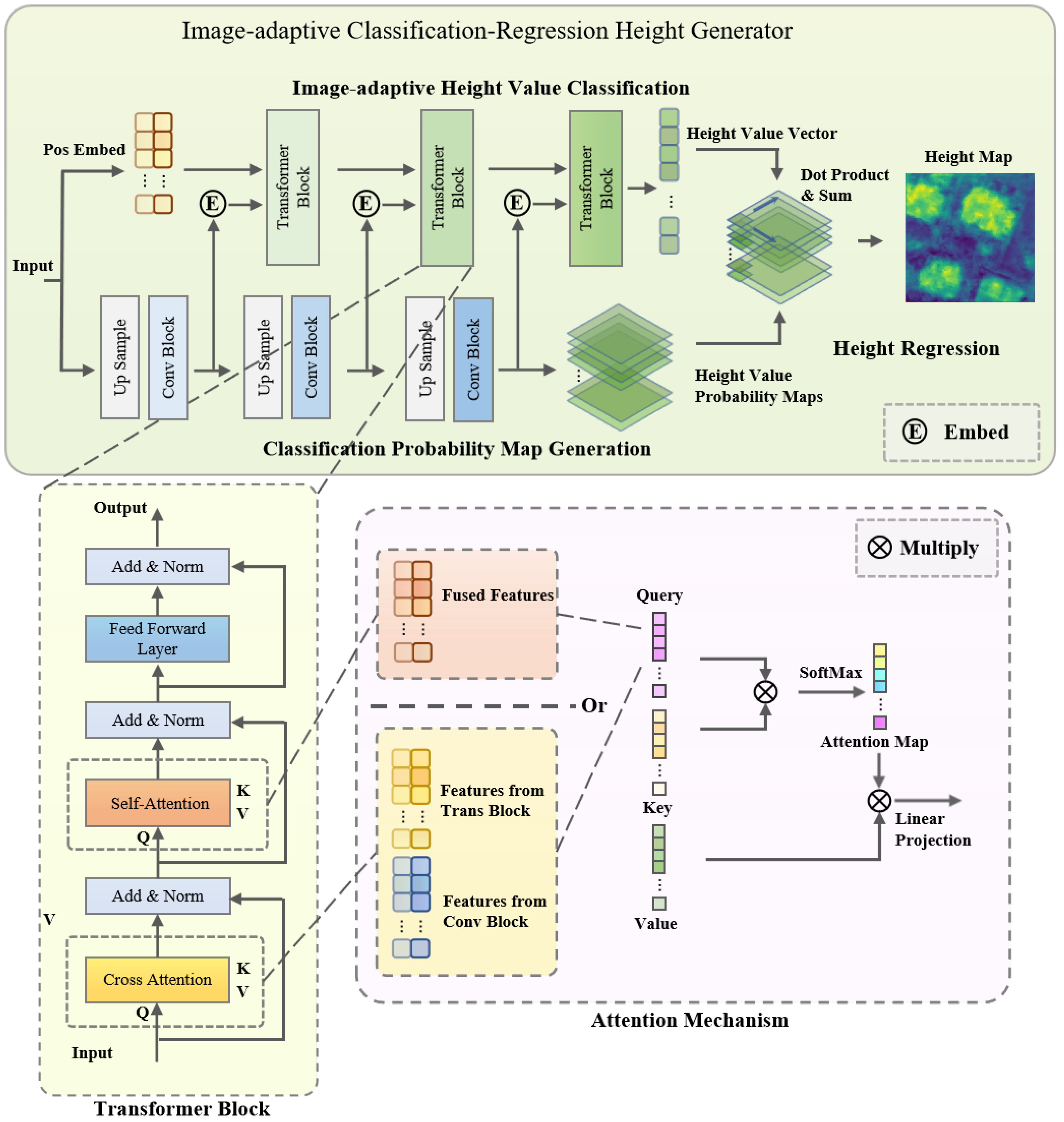
3.3. Image-Adaptive Classification–Regression Height Generator

Figure 6 illustrates the components of the Image-adaptive Classification–Regression Height Generator, encompassing Image-adaptive Height Value Classification, Classification Probability Map Generation, and Height Regression. During the encoder stage, the feature map size is continually refined for effective feature fusion. Correspondingly, in the decoder stage, with the input Y (H/16, W/16, 256N) from the encoder, multiscale feature maps are enhanced to achieve fine-grained modeling. Utilizing a Transformer Block and a Convolution Block at three distinct scales (H/16, W/16, 256N), (H/4, W/4, 16N), and (H, W, N), height values of the input image are categorized and height probability maps are produced. The height value regression is then obtained by calculating the product of height values and probability maps.

3.3.1. Image-adaptive Height Value Classification

In the Image-adaptive Height Value Classification component, the final output is a 1 × N height vector (denoted as H), comprising N height values, each representing a predicted category. The value N is set manually by researchers to divide the entire height range of the image into a specific number of distinct height values. To reduce the randomness of generated height values and increase affinity between the two branches, cross-attention is incorporated into the initial layer of the Transformer Block for further interaction with the probability graph branch (denoted as P). This means that the current Transformer Block layer accepts queries output from the previous layer and outputs embedded from the Conv Block on the same layer. The Transformer Block also includes addition and normalization, self-attention, and feedforward layer operations. If the current Transformer Block layer is the first layer, then the output of the previous Transformer Block is represented as $H^{l-1}$, and the input to the Conv Block is represented as $P^l$; the operation process is described as follows:

$${\widehat{H}}^l=LN(CA(H^{l-1},Embed\left(P^l\right))+H^{l-1})$$

(10)

$${\tilde{H}}^l=LN(MSA\left({\widehat{H}}^l\right)+{\widehat{H}}^l)$$

(11)

$$H^l=LN\left(FFL\left({\tilde{H}}^l\right)\right)+{\tilde{H}}^l)$$

(12)

The symbols $CA,MSA,LN$, and $FFL$, respectively, denote Cross-Attention, Multihead Self Attention, Layer Normalization, and Feedforward Layer operations.

3.3.2. Classification Probability Map Generation

For Classification Probability Map Generation, the process involves receiving a high channel feature map (256N) and outputting a height probability map of size (H, W, N). To adapt to the varied scale characteristics of aerial images, we designed a three-layer convolution pyramid structure with upsampling to continuously rebuild detail features. The Convolution Block includes UpSample, $Con{v}_{3\times 3}$, $Con{v}_{1\times 1}$, and $ReLu$; the output sizes of the three layers are (H/16, W/16, 16N), (H/4, W/4, 4N), and (H, W, N). If the current layer is denoted as l, and the input from the previous Convolution Block as $P^{l-1}$, the calculation process is

$${\widehat{P}}^l=ReLu\left(Con{v}_{3\times 3}\left(UpSample\left(P^{l-1}\right)\right)\right)$$

(13)

$$P^l=LN\left(Con{v}_{1\times 1}\left({\widehat{P}}^l\right)\right)$$

(14)

3.3.3. Height Regression

In the Height Regression phase, we first obtain the Height Vector (H) and the Height Value Probability Map (P) separately. Using SoftMax, we normalize both to fit within the 0–1 range. The height map of dimensions (H, W, 1) is then derived through the dot product operation. Finally, the height values are linearly scaled to align with the height range of the dataset, where the minimum and maximum height values of the dataset are represented by $h_{min}$ and $h_{max}$, respectively. The process is as follows:

$$\widehat{H}=SoftMax\left(H\right)$$

(15)

$$\widehat{P}=SoftMax\left(P\right)$$

(16)

$$\widehat{Result}=\sum _{i=1}^N({\widehat{H}}_i\times {\widehat{P}}_i)$$

(17)

$$Result=h_{min}+(h_{max}-h_{min})\times \widehat{Result}$$

(18)

3.4. Loss Function

We employ the sigmoid cross-entropy loss function, similar to other methodologies [51], which is precisely represented as follows:

$$g_i={log}_{}{\tilde{h}}_i-{log}_{}{h}_i$$

(19)

$$Loss=\alpha \sqrt{\frac{1}{T}{\displaystyle \sum _i}{g}_i^2-\frac{\lambda }{T^2}{\left({\displaystyle \sum _i}{g}_i\right)}^2}$$

(20)

Here, ${\tilde{h}}_i$, $h_i$, and T denote the estimated height, the actual height, and the number of valid pixels, respectively. Similar to Adabins [18], the parameters $\lambda$ and $\alpha$ are set to 0.85 and 10, respectively.

4. Experiment

4.1. Datasets

We utilized the ISPRS Vaihingen and Potsdam datasets for training and validation of our model, adhering to the official division of training and testing sets. The Vaihingen dataset includes 33 images, each approximately 2500 × 2500 pixels, with a pixel resolution of 0.09 m and a height range of 240.70–360.00 m. Following official recommendations, we linearly normalized the heights to a range of 0–1. Of the 33 images, 16 were used for training and 17 for testing. Additionally, we divided the larger single images into smaller 512 × 512 pixel segments for both training and testing. The Potsdam dataset consists of 38 images, each 6000 × 6000 pixels, with a pixel resolution of 0.05 m and a height range of −17.355–106.171 m. Of these, 24 images were designated for training and 14 for testing. We also performed height normalization and segmentation according to the official recommendations.

4.2. Metrics

The assessment metrics employed include prevalent indicators such as $Rel$, $RMSE\left(log\right)$, and threshold values $\delta 1$, $\delta 2$, $\delta 3$. Rel focuses on measuring average errors, while $RMSE\left(log\right)$ is more sensitive to outliers with substantial errors. Additionally, $\delta 1$, $\delta 2$, $\delta 3$ represent threshold accuracy metrics, assessing the proportion of pixels that maintain error control within a designated range, emphasizing overall error stability. These metrics are defined as follows:

$$Rel=\frac{1}{n}\sum \left|\frac{h_{pred}-h_{gt}}{h_{gt}}\right|$$

(21)

$$RMSE\left(log\right)=\sqrt{\frac{1}{n}\sum {(h_{pred}-h_{gt})}^2}$$

(22)

$${\delta }_i=Max(\frac{h_{pred}}{h_{gt}},\frac{h_{gt}}{h_{pred}})<1.{25}^i$$

(23)

Here, $h_{pred}$, $h_{gt}$, and n represent the predicted height map, the ground truth height map, and the number of pixels within the height map, respectively.

4.3. Experimental Settings

4.3.1. Hardware Platform and Libraries

The training component was executed on 4 Nvidia GeForce RTX 3090 GPUs, while a single RTX 3090 GPU was utilized for testing and comparison. Across these tasks, we employed the Ubuntu 22.04 system, nvidia-driver-525-server driver, CUDA 11.1 computing library, and the PyTorch 1.8.1 deep learning framework. Multi-threading mechanism like MMSegmentation handled the distributed computing across the 4 RTX 3090 GPUs. For the purpose of comparing parameter quantities, we did not make use of MMCV’s dynamic quantization capability.

4.3.2. Training

We train 24 epochs like Binsformer [51] and Depthformer [52] on both datasets running a batch size of 2 per GPU and initializing the learning rate at $1\times {10}^{-5}$. Utilizing the AdamW optimizer, we adjusted the learning rate throughout the training process. To circumvent early training instability, a warm-up period accounting for an eighth of the total training process was integrated during the initial phase.

4.3.3. Data Augmentation

We employed MMCV-provided data augmentation methods during the training phase. These include random image cropping to 448 × 448 dimensions, image rotation with a probability of 0.5 and a degree of 2.5, and both photometric and chromatic augmentations with a probability of 0.5, gamma range of 0.9 to 1.1, brightness range of 0.75 to 1.25, and color range of 0.9 to 1.1. Conversely, during the testing phase, we refrained from utilizing any data augmentation.

5. Results

5.1. Quantitative and Qualitative Analysis on Vaihingen

For the evaluation utilizing Vaihingen dataset, our proposed method, HeightFormer, was juxtaposed with existing models such as D3Net [38], Amirkolaee et al. [53], PSDNet [54], Li et al. [37], WMD [55], LeReS [56], ASSEH [57], Depthformer [52], Binsformer [51], and SFFDE [58] at

Table 1. Method comparison on the Vaihingen dataset. ↑: higher is better, ↓: lower is better.

Method	Ref	Rel↓	RMSE(log)↓	$\mathit{\delta }$1↑	$\mathit{\delta }$2↑	$\mathit{\delta }$3↑
D3Net [38]	ICIP 2018	2.016	-	-	-	-
Amirkolaee et al. [53]	ISPRS 2019	1.163	0.334	0.330	0.572	0.741
PSDNet [54]	CVPR 2020	0.363	0.171	0.447	0.745	0.906
Li et al. [37]	GRSL 2020	0.314	0.155	0.451	0.817	0.939
WMD [55]	CVPR 2021	0.272	-	0.543	0.798	0.916
LeReS [56]	CVPR 2021	0.260	-	0.554	0.800	0.932
ASSEH [57]	TGRS 2022	0.237	0.120	0.595	0.860	0.971
DepthFormer [52]	CVPR 2022	0.212	0.080	0.716	0.927	0.967
BinsFormer [51]	CVPR 2022	0.203	0.076	0.745	0.931	0.975
SFFDE [58]	TGRS 2023	0.222	0.084	0.595	0.897	0.970
HeightFormer	-	0.185	0.074	0.756	0.941	0.973

. Rel and RMSE(log) primarily quantify the average error in pixel prediction. HeightFormer, which integrates interaction ranges across various scales, achieves state-of-the-art performance. Metrics $\delta 1$, $\delta 2$, and $\delta 3$ determine the percentage of pixels with prediction errors within specific boundaries. The HeightFormer model, being compact, exhibits marginally larger height prediction errors for certain pixels, indicating that robustness warrants further enhancement. In terms of $\delta 3$, it slightly underperforms BinsFormer (0.973 < 0.975). A visual comparison between SFFDE and HeightFormer outcomes is also presented as Figure 7. Owing to its capacity to engage with global information, HeightFormer displays improved accuracy in height prediction for extensive scenes. As depicted in Figure 7c, this mitigates the instance-level bias issue inherent in convolutional networks.

5.2. Ablation Study on Vaihingen

In the ablation study section, we further tested the effectiveness of the Multilevel Interactive Backbone (MIB) and the Image-adaptive Classification–regression Height Generator (ICG) on Vaihingen.

5.2.1. Ablation of Multilevel Interaction Backbone (MIB)

Table 2. Ablation study with different modules of MIB on the Vaihingen dataset.

Pixel-	Patch-	HFC	Rel ↓	RMSE(log)↓	$\mathit{\delta }$1↑	$\mathit{\delta }$2↑	$\mathit{\delta }$3↑
√	-	-	0.281	0.113	0.564	0.794	0.947
-	√	-	0.203	0.077	0.624	0.895	0.959
√	√	√	0.185	0.074	0.756	0.941	0.973

HFC: heterogeneous feature coupling. ‘Pixel-’ refers to the convolutional backbone for extracting pixel-level features, ‘patch-’ denotes the local attention backbone for extracting patch-level features, and ‘HFC’ represents the channel-level attention module for extracting heterogeneous fused global features.

delineates the test outcomes derived from various interactional-level modules within the Multilevel Interactive Backbone (MIB). Evidenced by Line 1 of Table 2, the exclusive utilization of a pure convolution backbone network yields subpar performance metrics, while Column 4 in Figure 7 further demonstrates the arduousness of reconstructing comprehensive instances due to insufficient global information exchange. Prevailing state-of-the-art (SOTA) models, such as Binsformer [51], are constructed on the foundation of the transformer backbone, and correspondingly, Line 2 of Table 2 exhibits analogous performance benchmarks within our model. Ultimately, the HeightFormer effectively orchestrates disparate interaction modules, culminating in superior performance indicators and graphical representations.

5.2.2. Ablation of Image-Adaptive Classification–Regression Height Generator (ICG)

In the context of ICG, we assessed the efficacy of the image-adaptive height value approach and investigated its influence on model performance in relation to the various height value number settings. Figure 8 exemplifies this through the Rel indicator, demonstrating that the adaptive height strategy typically yields enhanced Rel indicator outcomes across distinct height value configurations, with other indicator performances detailed in

Table 3. Ablation study with different height value generation strategies of ICG on the Vaihingen dataset.

Type	N (Num of Height)	Rel↓	RMSE(log)↓	$\mathit{\delta }$1↑	$\mathit{\delta }$2↑	$\mathit{\delta }$3↑
Fixed	8	0.402	0.179	0.463	0.725	0.845
	16	0.356	0.156	0.502	0.747	0.859
	32	0.314	0.129	0.581	0.813	0.862
	64	0.288	0.118	0.619	0.846	0.877
	128	0.263	0.114	0.653	0.836	0.912
	256	0.267	0.118	0.639	0.826	0.920
Image-adaptive	8	0.341	0.135	0.458	0.742	0.903
	16	0.307	0.119	0.519	0.795	0.938
	32	0.203	0.076	0.714	0.935	0.965
	64	0.185	0.074	0.756	0.941	0.973
	128	0.191	0.075	0.737	0.921	0.967
	256	0.224	0.084	0.673	0.901	0.959

. With regard to visualization results, Columns 5 and 6 of Figure 7 reveal that, owing to an improved fit in height distribution for the corresponding input image, the adaptive height strategy exhibits discernible enhancements in edge detail restoration (yellow box) and noise suppression during instance reconstruction (gray box). In reference to the quantity of the height value (N), the Rel index for both methodologies experiences an initial decline, followed by stabilization as the count of height values escalates. Generally, exceedingly minimal height value settings resemble low-type classification tasks, thereby constraining modeling precision. Conversely, a profusion of height value settings approximates intricate regression endeavors, consequently amplifying the model’s complexity and impeding convergence. Ultimately, the HeightFormer attains peak efficacy at a proximal estimate of 64 height value settings. Owing to the constrained model fitting capacity inherent in fixed height settings, optimal performance is attained at an expanded height value configuration (approximately 128).

5.3. Method Comparison of the Computational Power Consumption

In

Table 4. Method comparison of model size and inference speed.

Method	Ref	Parameters	FPS
Li et al. [37]	GRSL 2020	-	8.7
DepthsFormer [52]	CVPR 2022	273 M	8.2
BinsFormer [51]	CVPR 2022	254 M	8.0
SFFDE [58]	TGRS 2023	>60 M	8.7
HeightFormer	-	46 M	10.8

, the parameter count and inference speed (frames per second, FPS) on a singular RTX 3090 for the most recent models are presented. Leveraging a lightweight backbone network and a multiscale reconstruction structure, HeightFormer outperforms with respect to both parameter quantity and end-point deployment requirements.

5.4. Quantitative and Qualitative Analysis on Potsdam

For the Potsdam dataset, a comparison of our proposed method, HeightFormer, was made with IMG2DSM, Amirkolaee et al. [53], BAMTL [59], DepthsFormer [52], and BinsFormer [51]. The properties of the Potsdam dataset are presented in

Table 5. Method comparison on the Potsdam dataset.

Method	Ref	Rel↓	RMSE(log)↓	$\mathit{\delta }$1↑	$\mathit{\delta }$2↑	$\mathit{\delta }$3↑
Amirkolaee et al. [53]	ISPRS 2019	0.571	0.259	0.342	0.601	0.782
BAMTL [59]	J-STARS 2020	0.291	-	0.685	0.819	0.897
DepthsFormer [52]	CVPR 2022	0.123	0.050	0.871	0.981	0.997
BinsFormer [51]	CVPR 2022	0.117	0.049	0.876	0.989	0.999
HeightFormer	-	0.104	0.043	0.893	0.987	0.997

, while the corresponding visualized results are illustrated in Figure 9. The comparison revealed that HeightFormer, much like in the case of Vaihingen, accomplished state-of-the-art results in terms of Rel, RMSE (log), $\delta 1$, $\delta 2$, reducing the relative error to approximately 10% (0.104) for the first time. Nevertheless, in terms of the metric $\delta 3$, HeightFormer scored a bit lower than BinsFormer (0.997 vs. 0.999). As inferred from the visualization, Figure 9a,c demonstrate that, constrained by monocular information input, HeightFormer still presents deviation in the reconstruction of plane texture height, with a tendency to recover height-independent details such as white lines on the football field and building shadows. It is notable in Figure 9d that HeightFormer exhibits considerable reconstruction noise for complex plane instances, indicating a requirement for further improvements in the model’s adaptability.

6. Conclusions

This study introduces HeightFormer, a novel technique for remote sensing monocular height estimation that employs multilevel interaction and image-adaptive classification–regression. Our proposed Multilevel Interaction Backbone (MIB) leverages attention mechanisms and the convolutional structure across various interactive scales to extract multiscale information concurrently. This approach effectively reduces the instance-level height biases common in pure convolutional architectures and the edge blurring issues found in ViT architectures, while controlling the model’s parameter count. Furthermore, we introduce an Image-adaptive Classification–Regression Height Generator (ICG) to reduce model convergence difficulty, enhance edge reconstruction quality, and lower the complexity of direct dense prediction modeling. We validated the effectiveness of our method using the ISPRS Vaihingen and Potsdam datasets, achieving relative errors of 0.185 and 0.104, respectively.

Considering that single-lens height estimation is inherently ill-posed, our HeightFormer model is compact and employs linear superimposition for height value generation. However, this leads to the presence of non-height-related textures in the generated results, as observed in Figure 9. In future work, we aim to refine the Height Regression component of ICG to mitigate the instability induced by unlearnable dot product operations. Additionally, we plan to explore incorporating multimodal inputs or multitask supervision mechanisms to enhance the model’s generalization ability through auxiliary input signals and supervisory labels.

References

1. Benediktsson, J.A.; Chanussot, J.; Moon, W.M. Very high-resolution remote sensing: Challenges and opportunities. Proc. IEEE 2012, 100, 1907–1910. [Google Scholar] [CrossRef]
2. Sun, X.; Wang, P.; Yan, Z.; Xu, F.; Wang, R.; Diao, W.; Chen, J.; Li, J.; Feng, Y.; Xu, T.; et al. FAIR1M: A benchmark dataset for fine-grained object recognition in high-resolution remote sensing imagery. ISPRS J. Photogramm. Remote. Sens. 2022, 184, 116–130. [Google Scholar] [CrossRef]
3. Zhao, L.; Wang, H.; Zhu, Y.; Song, M. A review of 3D reconstruction from high-resolution urban satellite images. Int. J. Remote Sens. 2023, 44, 713–748. [Google Scholar] [CrossRef]
4. Mahabir, R.; Croitoru, A.; Crooks, A.T.; Agouris, P.; Stefanidis, A. A critical review of high and very high-resolution remote sensing approaches for detecting and mapping slums: Trends, challenges and emerging opportunities. Urban Sci. 2018, 2, 8. [Google Scholar] [CrossRef]
5. Coronado, E.; Itadera, S.; Ramirez-Alpizar, I.G. Integrating Virtual, Mixed, and Augmented Reality to Human–Robot Interaction Applications Using Game Engines: A Brief Review of Accessible Software Tools and Frameworks. Appl. Sci. 2023, 13, 1292. [Google Scholar] [CrossRef]
6. Takaku, J.; Tadono, T.; Kai, H.; Ohgushi, F.; Doutsu, M. An Overview of Geometric Calibration and DSM Generation for ALOS-3 Optical Imageries. In Proceedings of the 2021 IEEE International Geoscience and Remote Sensing Symposium IGARSS, Brussels, Belgium, 11–16 July 2021; IEEE: Piscataway, NJ, USA, 2021; pp. 383–386. [Google Scholar]
7. Estornell, J.; Ruiz, L.; Velázquez-Martí, B.; Hermosilla, T. Analysis of the factors affecting LiDAR DTM accuracy in a steep shrub area. Int. J. Digit. Earth 2011, 4, 521–538. [Google Scholar] [CrossRef]
8. Nemmaoui, A.; Aguilar, F.J.; Aguilar, M.A.; Qin, R. DSM and DTM generation from VHR satellite stereo imagery over plastic covered greenhouse areas. Comput. Electron. Agric. 2019, 164, 104903. [Google Scholar] [CrossRef]
9. Hoja, D.; Reinartz, P.; Schroeder, M. Comparison of DEM generation and combination methods using high resolution optical stereo imagery and interferometric SAR data. Rev. Française Photogramm. Télédétect. 2007, 2006, 89–94. [Google Scholar]
10. Xiaotian, S.; Guo, Z.; Xia, W. High-precision DEM production for spaceborne stereo SAR images based on SIFT matching and region-based least squares matching. Int. Arch. Photogramm. Remote Sens. Spat. Inf. Sci. 2012, 39, 49–53. [Google Scholar] [CrossRef]
11. Li, Q.; Zhu, J.; Liu, J.; Cao, R.; Li, Q.; Jia, S.; Qiu, G. Deep learning based monocular depth prediction: Datasets, methods and applications. arXiv 2020, arXiv:2011.04123. [Google Scholar]
12. Kuznietsov, Y.; Stuckler, J.; Leibe, B. Semi-supervised deep learning for monocular depth map prediction. In Proceedings of the IEEE Conference on Computer Vision and Pattern Recognition, Honolulu, HI, USA, 21–26 July 2017; pp. 6647–6655. [Google Scholar]
13. Vaswani, A.; Shazeer, N.; Parmar, N.; Uszkoreit, J.; Jones, L.; Gomez, A.N.; Kaiser, Ł.; Polosukhin, I. Attention is all you need. Adv. Neural Inf. Process. Syst. 2017, 30, 1–11. [Google Scholar]
14. Zhao, S.; Luo, Y.; Zhang, T.; Guo, W.; Zhang, Z. A domain specific knowledge extraction transformer method for multisource satellite-borne SAR images ship detection. ISPRS J. Photogramm. Remote Sens. 2023, 198, 16–29. [Google Scholar] [CrossRef]
15. He, Q.; Sun, X.; Diao, W.; Yan, Z.; Yin, D.; Fu, K. Transformer-induced graph reasoning for multimodal semantic segmentation in remote sensing. ISPRS J. Photogramm. Remote Sens. 2022, 193, 90–103. [Google Scholar] [CrossRef]
16. Dosovitskiy, A.; Beyer, L.; Kolesnikov, A.; Weissenborn, D.; Zhai, X.; Unterthiner, T.; Dehghani, M.; Minderer, M.; Heigold, G.; Gelly, S.; et al. An image is worth 16x16 words: Transformers for image recognition at scale. arXiv 2020, arXiv:2010.11929. [Google Scholar]
17. Fu, H.; Gong, M.; Wang, C.; Batmanghelich, K.; Tao, D. Deep ordinal regression network for monocular depth estimation. In Proceedings of the IEEE Conference on Computer Vision and Pattern Recognition, Salt Lake City, UT, USA, 18–23 June 2018; pp. 2002–2011. [Google Scholar]
18. Bhat, S.F.; Alhashim, I.; Wonka, P. Adabins: Depth estimation using adaptive bins. In Proceedings of the IEEE/CVF Conference on Computer Vision and Pattern Recognition, Nashville, TN, USA, 20–25 June 2021; pp. 4009–4018. [Google Scholar]
19. Sun, W.; Zhang, Y.; Liao, Y.; Yang, B.; Lin, M.; Zhai, R.; Gao, Z. Rethinking Monocular Height Estimation From a Classification Task Perspective Leveraging the Vision Transformer. IEEE Geosci. Remote Sens. Lett. 2022, 19, 1–5. [Google Scholar] [CrossRef]
20. Wojek, C.; Walk, S.; Roth, S.; Schindler, K.; Schiele, B. Monocular visual scene understanding: Understanding multi-object traffic scenes. IEEE Trans. Pattern Anal. Mach. Intell. 2012, 35, 882–897. [Google Scholar] [CrossRef] [PubMed]
21. Goetz, J.; Brenning, A.; Marcer, M.; Bodin, X. Modeling the precision of structure-from-motion multi-view stereo digital elevation models from repeated close-range aerial surveys. Remote Sens. Environ. 2018, 210, 208–216. [Google Scholar] [CrossRef]
22. Geiger, A.; Lenz, P.; Stiller, C.; Urtasun, R. Vision meets robotics: The kitti dataset. Int. J. Robot. Res. 2013, 32, 1231–1237. [Google Scholar] [CrossRef]
23. Li, X.; Wen, C.; Wang, L.; Fang, Y. Geometry-aware segmentation of remote sensing images via joint height estimation. IEEE Geosci. Remote Sens. Lett. 2021, 19, 1–5. [Google Scholar] [CrossRef]
24. Mou, L.; Zhu, X.X. IM2HEIGHT: Height estimation from single monocular imagery via fully residual convolutional-deconvolutional network. arXiv 2018, arXiv:1802.10249. [Google Scholar]
25. Yu, D.; Ji, S.; Liu, J.; Wei, S. Automatic 3D building reconstruction from multi-view aerial images with deep learning. ISPRS J. Photogramm. Remote Sens. 2021, 171, 155–170. [Google Scholar] [CrossRef]
26. Mahdi, E.; Ziming, Z.; Xinming, H. Aerial height prediction and refinement neural networks with semantic and geometric guidance. arXiv 2020, arXiv:2011.10697. [Google Scholar]
27. Batra, D.; Saxena, A. Learning the right model: Efficient max-margin learning in laplacian crfs. In Proceedings of the 2012 IEEE Conference on Computer Vision and Pattern Recognition, Washington, DC, USA, 16–21 June 2012; IEEE: Piscataway, NJ, USA, 2012; pp. 2136–2143. [Google Scholar]
28. Saxena, A.; Chung, S.; Ng, A. Learning depth from single monocular images. Adv. Neural Inf. Process. Syst. 2005, 18, 1–16. [Google Scholar]
29. Saxena, A.; Schulte, J.; Ng, A.Y. Depth Estimation Using Monocular and Stereo Cues. In Proceedings of the IJCAI, Hyderabad, India, 6–12 January 2007; Volume 7, pp. 2197–2203. [Google Scholar]
30. Liu, M.; Salzmann, M.; He, X. Discrete-continuous depth estimation from a single image. In Proceedings of the IEEE Conference on Computer Vision and Pattern Recognition, Columbus, OH, USA, 23–28 June 2014; pp. 716–723. [Google Scholar]
31. Zhuo, W.; Salzmann, M.; He, X.; Liu, M. Indoor scene structure analysis for single image depth estimation. In Proceedings of the IEEE Conference on Computer Vision and Pattern Recognition, Boston, MA, USA, 7–12 June 2015; pp. 614–622. [Google Scholar]
32. Zhang, Y.; Yan, Z.; Sun, X.; Lu, X.; Li, J.; Mao, Y.; Wang, L. Bridging the Gap Between Cumbersome and Light Detectors via Layer-Calibration and Task-Disentangle Distillation in Remote Sensing Imagery. IEEE Trans. Geosci. Remote Sens. 2023, 61, 1–18. [Google Scholar] [CrossRef]
33. Zhang, Y.; Yan, Z.; Sun, X.; Diao, W.; Fu, K.; Wang, L. Learning efficient and accurate detectors with dynamic knowledge distillation in remote sensing imagery. IEEE Trans. Geosci. Remote Sens. 2021, 60, 1–19. [Google Scholar] [CrossRef]
34. He, K.; Zhang, X.; Ren, S.; Sun, J. Deep residual learning for image recognition. In Proceedings of the IEEE Conference on Computer Vision and Pattern Recognition, Las Vegas, NV, USA, 26 June–1 July 2016; pp. 770–778. [Google Scholar]
35. Ghamisi, P.; Yokoya, N. IMG2DSM: Height simulation from single imagery using conditional generative adversarial net. IEEE Geosci. Remote Sens. Lett. 2018, 15, 794–798. [Google Scholar] [CrossRef]
36. Zhang, Y.; Chen, X. Multi-path fusion network for high-resolution height estimation from a single orthophoto. In Proceedings of the 2019 IEEE International Conference on Multimedia & Expo Workshops (ICMEW), Shanghai, China, 8–12 July 2019; IEEE: Piscataway, NJ, USA, 2019; pp. 186–191. [Google Scholar]
37. Li, X.; Wang, M.; Fang, Y. Height estimation from single aerial images using a deep ordinal regression network. IEEE Geosci. Remote Sens. Lett. 2020, 19, 1–5. [Google Scholar] [CrossRef]
38. Carvalho, M.; Le Saux, B.; Trouvé-Peloux, P.; Almansa, A.; Champagnat, F. On regression losses for deep depth estimation. In Proceedings of the 2018 25th IEEE International Conference on Image Processing (ICIP), Athens, Greece, 7–10 October 2018; IEEE: Piscataway, NJ, USA, 2018; pp. 2915–2919. [Google Scholar]
39. Zhu, J.; Ma, R. Real-Time Depth Estimation from 2D Images. 2016. Available online: http://cs231n.stanford.edu/reports/2016/pdfs/407_Report.pdf (accessed on 1 December 2023).
40. Xiong, Z.; Huang, W.; Hu, J.; Zhu, X.X. THE benchmark: Transferable representation learning for monocular height estimation. IEEE Trans. Geosci. Remote Sens. 2023, 61, 5620514. [Google Scholar] [CrossRef]
41. Tao, H. A label-relevance multi-direction interaction network with enhanced deformable convolution for forest smoke recognition. Expert Syst. Appl. 2024, 236, 121383. [Google Scholar] [CrossRef]
42. Shaw, P.; Uszkoreit, J.; Vaswani, A. Self-attention with relative position representations. arXiv 2018, arXiv:1803.02155. [Google Scholar]
43. Jaderberg, M.; Simonyan, K.; Zisserman, A. Spatial transformer networks. arXiv 2015, arXiv:1506.02025. [Google Scholar]
44. Luong, M.T.; Pham, H.; Manning, C.D. Effective approaches to attention-based neural machine translation. arXiv 2015, arXiv:1508.04025. [Google Scholar]
45. Hu, J.; Shen, L.; Sun, G. Squeeze-and-excitation networks. In Proceedings of the IEEE Conference on Computer Vision and Pattern Recognition, Salt Lake City, UT, USA, 18–23 June 2018; pp. 7132–7141. [Google Scholar]
46. Huang, Z.; Wang, X.; Huang, L.; Huang, C.; Wei, Y.; Liu, W. Ccnet: Criss-cross attention for semantic segmentation. In Proceedings of the IEEE/CVF International Conference on Computer Vision, Seoul, Republic of Korea, 27 October–2 November 2019; pp. 603–612. [Google Scholar]
47. Liu, Z.; Lin, Y.; Cao, Y.; Hu, H.; Wei, Y.; Zhang, Z.; Lin, S.; Guo, B. Swin transformer: Hierarchical vision transformer using shifted windows. In Proceedings of the IEEE/CVF International Conference on Computer Vision, Montreal, BC, Canada, 11–17 October 2021; pp. 10012–10022. [Google Scholar]
48. Yang, J.; Du, B.; Zhang, L. From center to surrounding: An interactive learning framework for hyperspectral image classification. ISPRS J. Photogramm. Remote Sens. 2023, 197, 145–166. [Google Scholar] [CrossRef]
49. Chen, S.; Ogawa, Y.; Zhao, C.; Sekimoto, Y. Large-scale individual building extraction from open-source satellite imagery via super-resolution-based instance segmentation approach. ISPRS J. Photogramm. Remote Sens. 2023, 195, 129–152. [Google Scholar] [CrossRef]
50. He, Q.; Sun, X.; Yan, Z.; Wang, B.; Zhu, Z.; Diao, W.; Yang, M.Y. AST: Adaptive Self-supervised Transformer for optical remote sensing representation. ISPRS J. Photogramm. Remote Sens. 2023, 200, 41–54. [Google Scholar] [CrossRef]
51. Li, Z.; Wang, X.; Liu, X.; Jiang, J. Binsformer: Revisiting adaptive bins for monocular depth estimation. arXiv 2022, arXiv:2204.00987. [Google Scholar]
52. Li, Z.; Chen, Z.; Liu, X.; Jiang, J. Depthformer: Exploiting long-range correlation and local information for accurate monocular depth estimation. arXiv 2022, arXiv:2203.14211. [Google Scholar] [CrossRef]
53. Amirkolaee, H.A.; Arefi, H. Height estimation from single aerial images using a deep convolutional encoder-decoder network. ISPRS J. Photogramm. Remote Sens. 2019, 149, 50–66. [Google Scholar] [CrossRef]
54. Zhou, L.; Cui, Z.; Xu, C.; Zhang, Z.; Wang, C.; Zhang, T.; Yang, J. Pattern-structure diffusion for multi-task learning. In Proceedings of the IEEE/CVF Conference on Computer Vision and Pattern Recognition, Seattle, WA, USA, 14–19 June 2020; pp. 4514–4523. [Google Scholar]
55. Ramamonjisoa, M.; Firman, M.; Watson, J.; Lepetit, V.; Turmukhambetov, D. Single image depth prediction with wavelet decomposition. In Proceedings of the IEEE/CVF Conference on Computer Vision and Pattern Recognition, Nashville, TN, USA, 20–25 June 2021; pp. 11089–11098. [Google Scholar]
56. Yin, W.; Zhang, J.; Wang, O.; Niklaus, S.; Mai, L.; Chen, S.; Shen, C. Learning to recover 3d scene shape from a single image. In Proceedings of the IEEE/CVF Conference on Computer Vision and Pattern Recognition, Nashville, TN, USA, 20–25 June 2021; pp. 204–213. [Google Scholar]
57. Liu, W.; Sun, X.; Zhang, W.; Guo, Z.; Fu, K. Associatively segmenting semantics and estimating height from monocular remote-sensing imagery. IEEE Trans. Geosci. Remote Sens. 2022, 60, 1–17. [Google Scholar] [CrossRef]
58. Mao, Y.; Chen, K.; Zhao, L.; Chen, W.; Tang, D.; Liu, W.; Wang, Z.; Diao, W.; Sun, X.; Fu, K. Elevation Estimation-Driven Building 3D Reconstruction from Single-View Remote Sensing Imagery. IEEE Trans. Geosci. Remote Sens. 2023, 61, 5608718. [Google Scholar] [CrossRef]
59. Wang, Y.; Ding, W.; Zhang, R.; Li, H. Boundary-Aware Multitask Learning for Remote Sensing Imagery. IEEE J. Sel. Top. Appl. Earth Obs. Remote Sens. 2021, 14, 951–963. [Google Scholar] [CrossRef]
Figure 1. Typical problems of existing height estimation methods. (a): Instance-level height deviation caused by fixed receptive field. (b): Edge ambiguity (gray box: road; yellow box: building; green box: tree).
Remotesensing 16 00295 g001
Figure 2. Different interaction mechanism, (a): ViT-based global interaction mechanism. (b): Our multiscale interactive mechanism.
Remotesensing 16 00295 g002
Figure 3. Different height value generation method: Top, non-adaptive height values (N height values predetermined before model training as categories to be predicted); Bottom, adaptive height values (the categories of height values to be predicted for each image are generated by the current image, with more height values allocated to represent intervals where the data distribution of the current image is dense).
Remotesensing 16 00295 g003
Figure 4. Architecture of HeightFormer, consisting of Multilevel Interactive Backbone (MIB, three feature extraction modules ranging from coarse to fine) and Image-adaptive Classification–Regression Height Generator (ICG, branch-coupled image-adaptive mechanism).
Remotesensing 16 00295 g004
Figure 5. Architecture of Multilevel Interactive Backbone, mainly consisting of Convolution-Based Pixel Interaction Backbone, Transformer-Based Patch Interaction Backbone and Heterogeneous Feature Coupling.
Remotesensing 16 00295 g005
Figure 6. Architecture of Image-adaptive Classification–Regression Height Generator, consisting of Image-adaptive Height Value Classification and Classification Probability Map Generation.
Remotesensing 16 00295 g006
Figure 7. Visualization Results of Vaihingen (yellow box: edge; gray box: instance). (ac) includes three typical scenarios: crops, mixed roads, and buildings. From left to right: the monocular RGB input, the label, results of the latest SFFDE method, results of the encoder ablation experiment with only the convolutional backbone retained, results of the decoder ablation experiment using fixed height values, and the results of the complete HeightFormer.
Remotesensing 16 00295 g007
Figure 8. Ablation comparison with Rel between fixed height values and image-adaptive height values on the Vaihingen dataset.
Remotesensing 16 00295 g008
Figure 9. Visualization results of Potsdam. From left to right: the model’s monocular RGB inputs, the model’s labels and the results of the HeightFormer. (ad) represent planar, curved, and mixed scenes.
Remotesensing 16 00295 g009