Abstract
Monitoring excited hydroxyl (OH*) airglow is broadly used for characterizing the state and dynamics of the terrestrial atmosphere. Recently, the existence of excited hydroxyl was confirmed using satellite observations in the Martian atmosphere. The location and timing of its detection on Mars were restricted to a winter season at the north pole. We present three-dimensional global simulations of excited hydroxyl over a Martian year. The predicted spatio-temporal distribution of the OH* can provide guidance for future observations, namely by indicating where and when the airglow is likely to be detected.
1. Introduction
Airglow is a non-thermal emission by planetary atmospheres, which is not related to auroral effects, lightning, and meteor fireballs [1]. Burns [2,3,4] and Yntema [5] were the first to suggest the existence of an irradiating layer in the terrestrial atmosphere based on observations. Rayleigh [6] had shown that it was not associated with auroras. In the 1920s–1930s, the nature of the observed phenomenon was broadly discussed, and Chapman [7] was apparently the first to point out that exothermic chemical reactions are a source of excited atoms and molecules producing airglow. Further studies of all airglow emissions were slowed down by World War II but resumed with triple intensity due to new infrared and other emission-registration technologies developed for military purposes. The full history of this phenomenon is summarized in the overview by Hersé [8].
One of the most used observational methods for obtaining information about dynamics, temperature, and chemical composition in the terrestrial atmosphere is measuring OH* excited states emissions. Meinel [9,10] found lines of vibro-rotational transitions in atmospheric emissions, while Bates and Nicolet [11] suggested the exothermic reaction of ozone and hydrogen as a mechanism for populating vibrational levels of OH*. Krassovsky et al. [12,13,14,15] developed a theory for retrieving temperature and gravity wave parameters at the emissions’ peak altitude. Evans and Llewellyn [16] suggested a method of inferring atomic hydrogen concentrations from OH* emission. Based on Solar Mesosphere Explorer (SME) satellite measurements, Thomas [17] showed how this emission can be used for calculating atomic oxygen concentrations and applied it for studying seasonal variations in this minor component. Currently, observations of OH* emissions in the Earth’s mesopause are used in a range of applications, like quantifying atmospheric variability due to gravity waves (e.g., [18,19,20]), tides [21,22], and planetary waves [23,24]. The OH* emissions were utilized to study sudden stratospheric warming events [25,26] and the quasi-biennial oscillation [27]. Airglow emissions were used for assessing temperature trends and variations induced by the solar cycle (e.g., [28,29,30,31,32]), as well as the chemical composition in the mesopause region [33,34,35].
Hydroxyl emissions are not a strictly terrestrial phenomenon. They have been found on Venus [36,37,38] and Mars [39]. In the Venus atmosphere, OH* emissions were observed for the first time in March of 2007 [36] by the Visible and Infrared Thermal Imaging Spectrometer (VIRTIS) instrument onboard the Venus Express satellite [40]. Six years later, the OH* emissions were detected on Mars with Compact Reconnaissance Imaging Spectrometer for Mars (CRISM) aboard the Mars Reconnaissance Orbiter (MRO) in near-IR limb observations [39]. The OH* emissions for vibrational transitions 1-0, 2-1, and 2-0, with wavelengths 2.81, 2.94, and 1.42 μm, respectively, were detected in winter polar night areas (70–90°N/S) during Martian year 30 (MY30). The presence of OH* on these planets provides an opportunity to apply remote sensing techniques developed for Earth to studies of atmospheric processes there. At the moment, very little is known about spatio-temporal variations in hydroxyl emissions on these planets. This hinders the planning of new space missions and the development of instrumentation for detecting OH* airglow. Theoretical (modeling) investigations of OH* emissions in the Venus atmosphere were already performed in a number of works [41,42]. Our paper addresses this lack of knowledge by predicting where and when observations of OH* are possible in the Martian atmosphere based on model simulations.
2. Materials and Methods
We assume that the excited hydroxyl is in a photochemical equilibrium during night-time [43]. This assumption enables us to explicitly express the concentration of hydroxyl at all excitation levels [OHv] in the following form (see [44], Equation (1)):
where v is the vibrational number; is the nascent distribution [45]; is the reaction rate for the reaction of atomic hydrogen with ozone [46]; is the same for the reaction of excited hydroxyl with atomic oxygen [47]; and A, B, D, and G are the quenching coefficients by carbon dioxide [41], molecular oxygen [45], atomic oxygen [47], and molecular nitrogen [48], respectively. E represents the Einstein (spontaneous emission) coefficients from [49]. The square brackets denote the number densities of chemical species.
In Equation (1), the spontaneous emission, molecular, and atomic oxygen quenching are treated as multi-quantum phenomena; that is, they include relaxation from all the highest vibrational levels to all the lowest ones. Not all multi-quantum quenching coefficients are known. For instance, coefficients for quenching by molecular nitrogen and carbon dioxide have not been fully characterized, but only the so-called collisional cascade rates (where transitions occur to one level below) have been provided [50]. The most recent update on these coefficients has been presented by Krasnopolsky [41] for quenching by carbon dioxide and by Makhlouf et al. [48] for quenching by molecular nitrogen. We adopted these values from Krasnopolsky [41] and Makhlouf et al. [48] in our calculations to construct the diagonal matrix for Avv′ and Gvv′ for transitions v → v − 1, while we assign zero values to the non-diagonal terms for other transitions. Although argon and carbon monoxide are minor species in the Martian atmosphere, their concentrations are quite large. The quenching rates of excited hydroxyl by these species are not known thus far; therefore, we had to neglect them, just as it is usually performed for the Earth’s atmosphere.
Our OH* model does not include the reaction between hydroperoxy radicals (HO2) and atomic oxygen. This omission is justified by the limited significance of this reaction as a source for populating vibrationally excited hydroxyl levels [43,50,51,52]. At the initial stages of the study of hydroxyl emissions, the reaction of hydroperoxy radicals with atomic oxygen was introduced in order to reconcile the results of observations and modeling. With the acquisition of new knowledge about the processes of quenching, spontaneous emission, and quantum yield for the main reaction, there was no longer a need for the inclusion of this reaction in the consideration. In addition, there is no laboratory evidence of a significant OH* yield from this reaction. Therefore, we omitted it, following many other authors [53,54,55,56].
The model outlined above has been described in detail and compared with the available observations [39] in our previous studies [44,57]. It reproduces the values and shape of the CRISM observations for transitions 1-0 and 2-0 and shows ~30% lower values near the peak for transition 2-1. The latter is still within the CRISM’s uncertainty (see Figure 1c in [44] and Figure 7 in [39]). For transition 1-0, this result is better than the simulations with the Laboratoire de Météorologie Dynamique General Circulation Model (LMD GCM) and with the OH* models of Krasnopolsky [58] and García-Muñoz [43]. The latter two models overestimate the emission for this transition (Figure 1c in [44] and Figure 7 in [39]). For transition 2-0, all three models show similar values at the OH* peak (~5∙103 photons∙cm−3∙s−1), which are slightly larger than in the observed emission. The main differences between the current version and the previous one are the inclusion of the temperature dependence for quenching by atomic oxygen (D) and the incorporation of the reaction of excited hydroxyl with atomic oxygen (), as introduced in the work of Caridade et al. [47].
In order to calculate [OH*] from (1), we used concentrations of all chemical constituents (O3, O, H, O2, N2, CO2), air density, and temperature from the Mars Climate Database (MCD), which is based on simulations with the Mars Planetary Climate Model (formerly the LMD GCMl) [59,60]. The latter is a three-dimensional model with a resolution of 64 longitudinal, 48 latitudinal, and 32 vertical grid points covering altitudes from the ground to ~120 km. We calculated OH* distributions at each grid point using Equation (1). In particular, the MCD includes the concentration of ozone [61], which is directly involved in OH* production; water vapor [62], which is the principal source of odd hydrogens (H, OH, HO2); and other long-lived species (carbon dioxide, atomic oxygen, molecular oxygen, and molecular nitrogen) involved in quenching processes. We utilized the data for Martian year 30, which is characterized by rather low dust [63] and solar activities. Investigation of the impact of dust storms and solar activity on hydroxyl emissions deserves a separate study and is out of the scope of this paper. We calculated the OH* according to Equation (1) at 00:00 LT and 12:00 LT (local midnight and midday, correspondingly) and averaged over all such longitudes during a sol. Thus, night- and daytime values refer to the local time rather than to insolation, as Equation (1) is applicable to all solar zenith angles (insolation conditions).
3. Results
The decline in the concentration of excited hydroxyl with an increase in vibrational number was found using modeling and observations in the Earth’s atmosphere [45,48,50,52,64]. Modeling OH* for the Martian atmosphere shows a similar result, which has been explained theoretically [43,44,57]. Since OH* concentrations increase with decreasing vibrational number, the strongest volume emission is produced by OH* with the lowest vibrational numbers, as is seen from modeling and observations [39,44,57]. Note that observations show a similar volume emission for transitions 2→1 and 1→0. For certainty, we consider only concentrations of OH* with the vibrational number one.
Different instruments have different sensitivities and uncertainties. Therefore, there is no sense in focusing on a particular one. Instead, we introduce a possible detection threshold. The CRISM instrument detected OH* emissions with absolute values above 103 photons∙cm−3∙s−1 with acceptable uncertainties depending on the wavelength. For the first two vibrational numbers, this corresponds to the OH* concentration of ~102 cm−3.
We consider the concentration cm−3 as a detectability threshold because the corresponding volume emission for the 1-0 transition is photons∙cm−3∙s−1 (E10 = 17.6 s−1, [49]). This emission is practically guaranteed to be measured with an acceptable accuracy.
Figure 1 presents the calculated seasonal variations in the night-time mean (averaged over a sol) at several latitudes, while Figure 2 illustrates its latitudinal structure during different seasons. The red solid lines in the figures indicate the peak of the layer, while the threshold value cm−3 is shown with the white dashed line. It is seen that the distributions are not fully periodic functions of Ls. This is a consequence of using the MCD data for a specific year (MY30), which are affected by the inter-annual variability. It is also seen from Figure 1a,e and Figure 2 that the largest concentrations occur at high northern latitudes (≥60°N) in the second half of the Martian year (LS = 180–360°) and at high southern latitudes (≥60°S) in the first half (LS = 0–180°). The concentration reaches more than 103 cm−3 and is located at altitudes of ~45–55 km. The hydroxyl peak extends to the maximum height of 75 km in northern mid-latitudes (~40°N) and in high southern latitudes (≥60°S), both around the perihelion season LS = 270° with concentrations of several tens of cm−3. The lowest height of the peak is ~42 km, which occurs in high southern (≥60°S) and equatorial latitudes near the aphelion (LS = 90°) with values of more than 103 cm−3 and at ~30°S during the northern spring equinox (LS = 0°) with values of a few hundred cm−3.
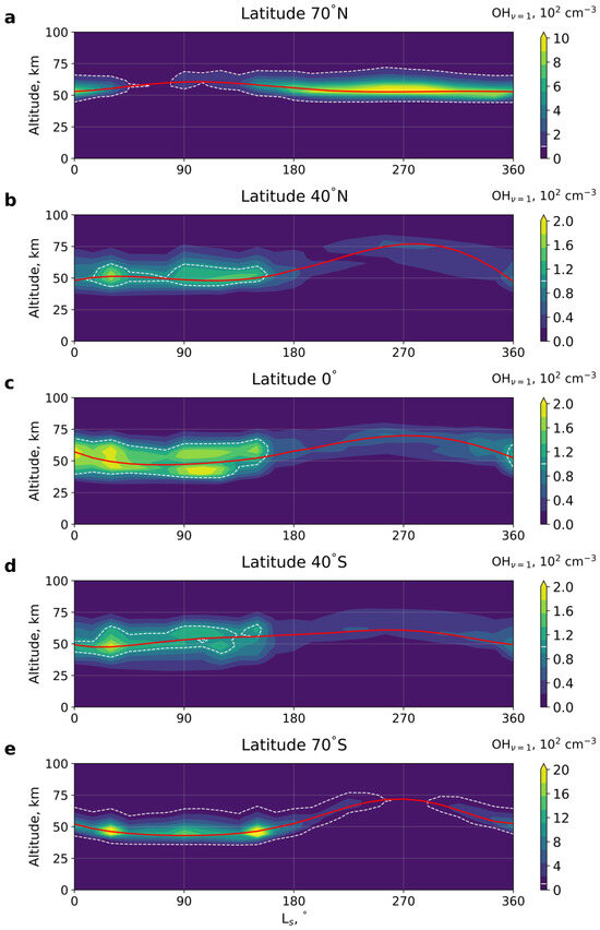
Figure 1.
Seasonal variation in the night-time mean (averaged over a sol) at different latitudes: (a) 70°N, (b) 40°N, (c) 0°, (d) 40°S, (e) 70°S. LS denotes the solar longitude. Red solid line indicates the peak of the layer. White dashed line shows the threshold value cm−3.
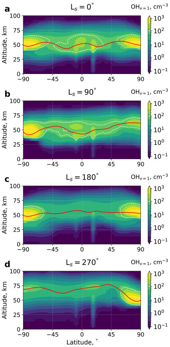
Figure 2.
Latitudinal structure of the night-time mean (averaged over a sol) at different seasons: (a) LS = 0°, (b) LS = 90°, (c) LS = 180°, (d) LS = 270°. As in Figure 1, the red solid line denotes the peak of the layer, and the white dashed line represents the threshold value cm−3. LS indicates the solar longitude.
Since OH* concentrations depend on atomic oxygen and temperature, we plotted Figure 3 for illustrative purposes to show the temperature (left column) and atomic oxygen (right column) for spring (first row), summer (second row), fall (third row), and winter (last row).
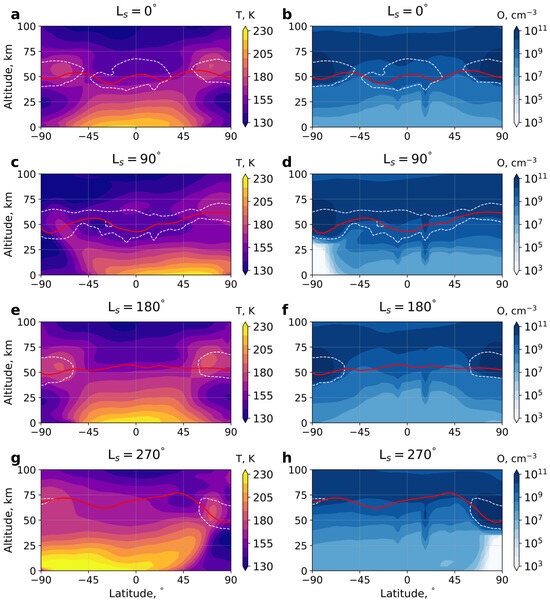
Figure 3.
Latitudinal structure of the night-time zonal mean temperature and atomic oxygen concentrations at different seasons: (a,b) LS = 0°, (c,d) LS = 90°, (e,f) LS = 180°, (g,h) LS = 270°. As in Figure 1 and Figure 2, the red solid line denotes the peak of the layer, and the white dashed line represents the threshold value cm−3. LS denotes the solar longitude.
Figure 4 presents the computed seasonal-latitudinal cross-sections of [OH1] concentrations at the height of the peak values in the Martian atmosphere for (a) night-time and (b) daytime conditions, along with the peak height itself at (c) night and (d) daytime. The white dashed line denotes regions where concentrations exceed the threshold required for detection.
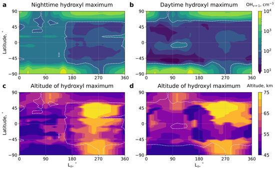
Figure 4.
The calculated seasonal-latitudinal variation in concentrations in Martian atmosphere at night-time (a) and daytime (b) conditions, and the height at the peak of the layer for night (c) and day (d). White dashed line shows the threshold value cm−3. LS denotes the solar longitude.
4. Discussion
There are similarities and differences in the variations in the nocturnal hydroxyl on Mars and in the terrestrial mesosphere. The figures demonstrate that the peak on Mars varies by ~30 km between ~45 and 75 km. On Earth, the variations are much narrower and amount to only about 10 km (e.g., [65] and references therein). On Mars, the largest vertical variation is predicted near northern mid-latitudes (~40°N) and southern high latitudes (70°S) (Figure 1b,e). The terrestrial OH* airglow layer varies annually and semiannually [22,27,66,67], whereas on Mars, only the annual cycle is seen. Unlike in the Earth’s mesopause, the annual variations on Mars demonstrate no latitudinal symmetry with respect to the equator, except at high latitudes (Figure 1a,e). Providing an explanation for the fluctuations in OH* is beyond the scope of this paper. Such a study could be carried out using the approach published in the previous works [44,57], where it was shown that if ozone is in chemical equilibrium, the concentration of OH* is proportional to that of atomic oxygen and air density and inversely proportional to the power of temperature (~1/T2.4). Thus, variations in the hydroxyl layer are ultimately determined by variations in these three components. Moreover, variations in air density and atomic oxygen concentrations were found to be primary factors, while variations in temperature contribute less. In case of strong deviations in ozone from chemical equilibrium, variations in OH* can be considered only in terms of components directly involved in its formation, i.e., of ozone and atomic hydrogen. Therefore, it is important to establish with certainty the times and locations where the photochemical equilibrium of ozone holds before considering factors contributing to the OH* variations.
Near the terrestrial mesopause, the concentration of excited hydroxyl at the peak anticorrelates with its altitude [27,68,69]. Figure 1 demonstrates a similar inverse correlation on Mars. This relationship was theoretically predicted under the assumption of ozone being in photochemical equilibrium [44,57]. The expression for the peak altitude was derived in [44,57]. It shows that the altitude depends on the amount of atomic oxygen, temperature, and their vertical gradients (see Equation (9) in [44,57]). However, it is important to note that such an inverse correlation can occur without photochemical equilibrium as well.
The full width at half maximum layer on Mars can be as large as 20–25 km, while on Earth, it is approximately 8–10 km [70]. This implies that the Martian OH* layer is broader and that retrieving minor chemical species like atomic oxygen and atomic hydrogen would be possible over a wider range of altitudes.
Another similarity between the excited hydroxyl in the Martian and terrestrial atmospheres is the formation of double-maxima structures, as seen in Figure 1c and Figure 2b,d. This phenomenon has been reported in the terrestrial mesopause in several studies [71,72]. Such structures are formed because [OH*] is directly proportional to the concentration of atomic oxygen and inversely proportional to the power of temperature. Consequently, one maximum of OH* can occur near the peak of O and the other forms near the temperature minimum. Similar reasons can explain the double structure on Mars.
By comparing Figure 2 and Figure 3, one can see that large values of OH* concentrations occur when atomic oxygen concentrations are large, even though the temperature is also large in these regions (high and middle latitudes). In previous works, it was shown that atomic oxygen plays a primary role in OH* formation [44,57]. Regions of high hydroxyl concentration can be formed when the amount of atomic oxygen is not the largest, but the temperature is low, as, for example, in the equatorial and low latitudes in spring and summer (Figure 3a–d). We do not present a more extensive analysis of the impacts of temperature and atomic oxygen because this question is out of the scope of the current study. Nevertheless, we note that it can be achieved either by utilizing the decomposition approach from [44,57] or by conducting numerical experiments with constant (averaged) temperature and variable [O], and vice versa.
It is seen in Figure 4 that, during night-time, the detection of excited hydroxyl on Mars is feasible at middle and low latitudes in the first half of the year, up to LS = 160°, and at high latitudes during almost all seasons, except for a one-month period in the summer hemispheres around LS = 70° and LS = 270°. The areas near LS = 70° and LS = 270° at high latitudes correspond to the polar day, where ozone (directly involved in OH* formation) is reduced via dissociation. During daytime, detection is only possible at high latitudes, where OH* concentrations closely resemble night-time values, and diurnal variability is either nonexistent or very weak. This fact suggests that ozone may not be in a photochemical equilibrium in this region but rather behaves as a passive tracer, similar to what occurs in the stratosphere of Earth. However, this aspect requires further in-depth exploration and is out of the scope of this paper.
5. Conclusions
In this paper, we characterized the main features of the excited hydroxyl (OH*) morphology in the Martian atmosphere obtained from modeling and discussed the similarities and differences in the latitudinal-seasonal variations in OH* in the terrestrial atmosphere. The three-dimensional distributions of OH* were calculated using concentrations of chemical species, air density, and temperature from the Mars Planetary Climate Model (formerly the Laboratoire de Météorologie Dynamique General Circulation Model) for MY30. The comparison of the model’s results with observations has been presented in past works [44,57].
Measurements of the excited hydroxyl airglow can be used for obtaining information on minor chemical species, for studying variations in temperature and dynamics. The main conclusion of our work is that the night-time detection of hydroxyl is possible at high latitudes (above ~60°) throughout the year, with the exception of a short period of about one Martian month in the summer hemispheres with LS = 70° and LS = 270°, which correspond to the polar day regions. At middle and equatorial latitudes (from ~60°S to ~60°N, see Figure 4), hydroxyl can be detected from LS = 0° to LS = 160°. The detection of hydroxyl in the daytime is likely to be very difficult at middle and equatorial latitudes through the entire year and is more feasible at high latitudes, except for a short period around LS = 70° and LS = 270° (under the polar day conditions).
Finally, we note that because the atmospheres of Venus and Mars are both CO2-dominated and processes of formation and deactivation of OH* are identical on both planets, the presented approach can be directly applied to the Venusian atmosphere as well.
Author Contributions
Conceptualization, D.S.S., M.G., A.S.M., G.R.S. and P.H.; investigation, D.S.S., M.G., A.S.M., G.R.S. and P.H.; methodology, D.S.S., M.G., A.S.M., G.R.S. and P.H.; software, D.S.S. and M.G.; validation, D.S.S., M.G., A.S.M., G.R.S. and P.H.; visualization, D.S.S.; writing—original draft, D.S.S., M.G., A.S.M., G.R.S. and P.H.; writing—review and editing, D.S.S., M.G., A.S.M., G.R.S. and P.H. All authors have read and agreed to the published version of the manuscript.
Funding
This study received partial funding from a grant 23-72-01009 provided by the Russian Science Foundation.
Data Availability Statement
The MCD data were sourced from the website (http://www-mars.lmd.jussieu.fr/, accessed on 21 September 2023). The calculated results are accessible at https://doi.org/10.5281/zenodo.10407641 (accessed on 21 September 2023).
Acknowledgments
The authors are grateful to the LMD-GCM team for data availability.
Conflicts of Interest
The authors declare no conflicts of interest. The funders had no role in the design of the study; in the collection, analyses, or interpretation of data; in the writing of the manuscript; or in the decision to publish the results.
References
- Chamberlain, J.W. Physics of the Aurora and Airglow; Academic Press: New York, NY, USA, 1961. [Google Scholar]
- Burns, G.J. The Light of the Sky. J. Br. Astron. Assoc. 1906, 16, 308–309. [Google Scholar]
- Burns, G.J. Earthlight. Observatory 1910, 33, 169–172. [Google Scholar]
- Burns, G.J. The Total Amount of Starlight and the Brightness of the Sky. Observatory 1910, 33, 123–129. [Google Scholar]
- Yntema, L. On the Brightness of the Sky and Total Amount of Starlight. Publ. Astron. Lab. Groningen 1909, 22, 1–55. [Google Scholar]
- Rayleigh, L. On a night sky of exceptional brightness, and on the distinction between the polar aurora and the night sky. Proc. R. Soc. Lond. 1931, A131, 376–381. [Google Scholar]
- Chapman, S. The absorption and dissociative or ionizing effect of monochromatic radiation in an atmosphere on a rotating earth. Proc. Phys. Soc. 1931, 43, 26. [Google Scholar] [CrossRef]
- Hersé, M. Bright nights; past, present, and future trends. In Geophysical Research; Schröder, W., Ed.; Interdivisional Commission on History of IAGA: Potsdam, Germany, 1988; pp. 41–64. [Google Scholar]
- Meinel, A.B. OH Emission Bands in the Spectrum of the Night Sky II. Astrophys. J. 1950, 112, 120. Available online: https://adsabs.harvard.edu/pdf/1950ApJ...112..120M (accessed on 12 January 2023). [CrossRef]
- Meinel, A.B. OH Emission Bands in the Spectrum of the Night Sky I. Astrophys. J. 1950, 111, 555. Available online: https://adsabs.harvard.edu/pdf/1950ApJ...111..555M (accessed on 12 January 2023). [CrossRef]
- Bates, D.R.; Nicolet, M. The photochemistry of atmospheric water vapor. J. Geophys. Res. 1950, 55, 301–327. [Google Scholar] [CrossRef]
- Krassovsky, V.I. Sky and Polar Light Radiation (From the IGY program).(Rus.). Bull. Acad. Sci. USSR 1956, 5, 29–31. [Google Scholar]
- Krassovsky, V.I. On the remarks of DR Bates and BL Moiseiwitsch (1956) regarding the O3 and O1∗ hypotheses of the excitation of the OH airglow. J. Atmos. Terres. Phys. 1957, 10, 49–51. [Google Scholar] [CrossRef]
- Krassovsky, V.; Truttse, Y.; Shefov, N. Institute of Physics of the Atmosphere of the USSR Academy of Sciences, Moscow, USSR. Space Res. 1965, 5, 43. [Google Scholar]
- Krassovsky, V.I.; Shefov, N.N.; Vaisberg, O.L. Atomic hydrogen and helium in the airglow. Ann. Geophys. 1966, 22, 138–146. [Google Scholar]
- Evans, W.F.J.; Llewellyn, E.J. Atomic hydrogen concentrations in the mesosphere and the hydroxyl emissions. J. Geophys. Res. 1973, 78, 323–326. [Google Scholar] [CrossRef]
- Thomas, R.J. Atomic hydrogen and atomic oxygen density in the mesosphere region: Global and seasonal variations deduced from Solar Mesosphere Explorer near-infrared emissions. J. Geophys. Res. 1990, 95, 16457–16476. [Google Scholar] [CrossRef]
- Taylor, M.J.; Espy, P.J.; Baker, D.J.; Sica, R.J.; Neal, P.C.; Pendleton, W.R., Jr. Simultaneous intensity, temperature and imaging measurements of short period wave structure in the OH nightglow emission. Planet. Space Sci. 1991, 39, 1171–1188. [Google Scholar] [CrossRef]
- Shepherd, G.G.; Thuillier, G.; Cho, Y.-M.; Duboin, M.-L.; Evans, W.F.J.; Gault, W.A.; Hersom, C.; Kendall, D.J.W.; Lathuillère, C.; Lowe, R.P.; et al. The Wind Imaging Interferometer (WINDII) on the Upper Atmosphere Research Satellite: A 20 year perspective. Rev. Geophys. 2012, 50, RG2007. [Google Scholar] [CrossRef]
- Wachter, P.; Schmidt, C.; Wüst, S.; Bittner, M. Spatial gravity wave characteristics obtained from multiple OH(3–1) airglow temperature time series. J. Atmos. Sol. Terr. Phys. 2015, 135, 192–201. [Google Scholar] [CrossRef]
- Lopez-Gonzalez, M.J.; Rodríguez, E.; Shepherd, G.G.; Sargoytchev, S.; Shepherd, M.G.; Aushev, V.M.; Brown, S.; García-Comas, M.; Wiens, R.H. Tidal variations of O2 Atmospheric and OH(6-2) airglow and temperature at mid-latitudes from SATI observations. Ann. Geophys. 2005, 23, 3579–3590. [Google Scholar] [CrossRef]
- Xu, J.; Smith, A.K.; Jiang, G.; Gao, H.; Wei, Y.; Mlynczak, M.G.; Russell, J.M., III. Strong longitudinal variations in the OH nightglow. Geophys. Res. Lett. 2010, 37, L21801. [Google Scholar] [CrossRef]
- Buriti, R.A.; Takahashi, H.; Lima, L.M.; Medeiros, A.F. Equatorial planetary waves in the mesosphere observed by airglow periodic oscillations. Adv. Space Res. 2005, 35, 2031–2036. [Google Scholar] [CrossRef]
- Lopez-Gonzalez, M.J.; Rodríguez, E.; García-Comas, M.; Costa, V.; Shepherd, M.G.; Shepherd, G.G.; Aushev, V.M.; Sargoytchev, S. Climatology of planetary wave type oscillations with periods of 2-20 days derived from O2 atmospheric and OH(6-2) airglow observations at mid-latitude with SATI. Ann. Geophys. 2009, 27, 3645–3662. [Google Scholar] [CrossRef]
- Shepherd, M.G.; Cho, Y.-M.; Shepherd, G.G.; Ward, W.; Drummond, J.R. Mesospheric temperature and atomic oxygen response during the January 2009 major stratospheric warming. J. Geophys. Res. 2010, 115, A07318. [Google Scholar] [CrossRef]
- Shepherd, M.G.; Meek, C.E.; Hocking, W.K.; Hall, C.M.; Partamies, N.; Sigernes, F.; Manson, A.H.; Ward, W.E. Multi-instrument study of the mesosphere-lower thermosphere dynamics at 80°N during the major SSW in January 2019. J. Atmos. Sol. Terr. Phys. 2020, 210, 105427. [Google Scholar] [CrossRef]
- Gao, H.; Xu, J.; Wu, Q. Seasonal and QBO variations in the OH nightglow emission observed by TIMED/SABER. J. Geophys. Res. 2010, 115, A06313. [Google Scholar] [CrossRef]
- Bittner, M.; Offermann, D.; Graef, H.-H.; Donner, M.; Hamilton, K. An 18 year time series of OH rotational temperatures and middle atmosphere decadal variations. J. Atmos. Sol. Terr. Phys. 2002, 64, 1147–1166. [Google Scholar] [CrossRef]
- Espy, P.J.; Stegman, J.; Forkman, P.; Murtagh, D. Seasonal variation in the correlation of airglow temperature and emission rate, Geophys. Res. Lett. 2007, 34, L17802. [Google Scholar] [CrossRef]
- Pertsev, N.; Perminov, V. Response of the mesopause airglow to solar activity inferred from measurements at Zvenigorod, Russia. Ann. Geophys. 2008, 26, 1049–1056. [Google Scholar] [CrossRef]
- Dalin, P.; Perminov, V.; Pertsev, N.; Romejko, V. Updated long-term trends in mesopause temperature, airglow emissions, and noctilucent clouds. J. Geophys. Res. 2020, 125, e2019JD030814. [Google Scholar] [CrossRef]
- Perminov, V.I.; Pertsev, N.N.; Dalin, P.A.; Zheleznov, Y.A.; Sukhodoev, V.A.; Orekhov, M.D. Seasonal and Long-Term Changes in the Intensity of O2(b1Σ) and OH(X2Π) Airglow in the Mesopause Region. Geomagn. Aeron. 2021, 61, 589–599. [Google Scholar] [CrossRef]
- Russell, J.P.; Ward, W.E.; Lowe, R.P.; Roble, R.G.; Shepherd, G.G.; Solheim, B. Atomic oxygen profiles (80 to 115 km) derived from Wind Imaging Interferometer/Upper Atmospheric Research Satellite measurements of the hydroxyl and greenline airglow: Local time–latitude dependence. J. Geophys. Res. 2005, 110, D15305. [Google Scholar] [CrossRef]
- Mlynczak, M.G.; Hunt, L.A.; Mast, J.C.; Marshall, B.T.; Russell, J.M., III; Smith, A.K.; Siskind, D.E.; Yee, J.-H.; Mertens, C.J.; Martin-Torres, F.J.; et al. Atomic oxygen in the mesosphere and lower thermosphere derived from SABER: Algorithm theoretical basis and measurement uncertainty. J. Geophys. Res. 2013, 118, 5724–5735. [Google Scholar] [CrossRef]
- Mlynczak, M.G.; Hunt, L.A.; Marshall, B.T.; Mertens, C.J.; Marsh, D.R.; Smith, A.K.; Russell, J.M.; Siskind, D.E.; Gordley, L.L. Atomic hydrogen in the mesopause region derived from SABER: Algorithm theoretical basis, measurement uncertainty, and results. J. Geophys. Res. 2014, 119, 3516–3526. [Google Scholar] [CrossRef]
- Piccioni, G.; Drossart, P.; Zasova, L.; Migliorini, A.; Gérard, J.-C.; Mills, F.P.; Shakun, A.; García Muñoz, A.; Ignatiev, N.; Grassi, D.; et al. First detection of hydroxyl in the atmosphere of Venus. Astron. Astrophys. 2008, 483, L29–L33. [Google Scholar] [CrossRef]
- Gérard, J.-C.; Soret, L.; Saglam, A.; Piccioni, G.; Drossart, P. The distributions of the OH Meinel and O2(a1Δ − X3Σ) nightglow emissions in the Venus mesosphere based on VIRTIS observations. Adv. Space Res. 2010, 45, 1268–1275. [Google Scholar] [CrossRef]
- Soret, L.; Gérard, J.-C.; Piccioni, G.; Drossart, P. Venus OH nightglow distribution based on VIRTIS limb observations from Venus Express. Geophys. Res. Lett. 2010, 37, L06805. [Google Scholar] [CrossRef]
- Clancy, R.T.; Sandor, B.J.; García-Muñoz, A.; Lefèvre, F.; Smith, M.D.; Wolff, M.J.; Montmessin, F.; Murchie, S.L.; Nair, H. First detection of Mars atmospheric hydroxyl: CRISM Near-IR measurement versus LMD GCM simulation of OH Meinel band emission in the Mars polar winter atmosphere. Icarus 2013, 226, 272–281. [Google Scholar] [CrossRef]
- Drossart, P.; Piccioni, G.; Adriani, A.; Angrilli, F.; Arnold, G.; Baines, K.H.; Bellucci, G.; Benkhoff, J.; Bézard, B.; Bibring, J.P.; et al. Scientific goals for the observation of Venus by VIRTIS on ESA/Venus express mission. Planet. Space Sci. 2007, 55, 1653–1672. [Google Scholar] [CrossRef]
- Krasnopolsky, V.A. Nighttime photochemical model and night airglow on Venus. Planet. Space Sci. 2013, 85, 78–88. [Google Scholar] [CrossRef]
- Parkinson, C.D.; Bougher, S.W.; Mills, F.; Yung, Y.L.; Brecht, A.; Shields, D.; Liemohn, M. Modeling of observations of the OH nightglow in the venusian mesosphere. Icarus 2021, 368, 114580. [Google Scholar] [CrossRef]
- García-Muñoz, A.; McConnell, J.C.; McDade, I.C.; Melo, S.M.L. Airglow on Mars: Some model expectations for the OH Meinel bands and the O2 IR atmospheric band. Icarus 2005, 176, 75–95. [Google Scholar] [CrossRef]
- Grygalashvyly, M.; Shaposhnikov, D.S.; Medvedev, A.S.; Sonnemann, G.R.; Hartogh, P. Simplified Relations for the Martian Night-Time OH* Suitable for the Interpretation of Observations. Remote Sens. 2022, 14, 3866. [Google Scholar] [CrossRef]
- Adler-Golden, S. Kinetic parameters for OH nightglow modeling consistent with recent laboratory measurements. J. Geophys. Res. 1997, 102, 19969–19976. [Google Scholar] [CrossRef]
- Burkholder, J.B.; Sander, S.P.; Abbatt, J.; Barker, J.R.; Cappa, C.; Crounse, J.D.; Dibble, T.S.; Huie, R.E.; Kolb, C.E.; Kurylo, M.J.; et al. Chemical Kinetics and Photochemical Data for Use in Atmospheric Studies, Evaluation No. 19; JPL Publication 19-5; Jet Propulsion Laboratory: Pasadena, CA, USA, 2020. Available online: http://jpldataeval.jpl.nasa.gov (accessed on 21 September 2023).
- Caridade, P.J.S.B.; Horta, J.-Z.J.; Varandas, A.J.C. Implications of the O + OH reaction in hydroxyl nightglow modeling. Atmos. Chem. Phys. 2013, 13, 1–13. [Google Scholar] [CrossRef]
- Makhlouf, U.B.; Picard, R.H.; Winick, J.R. Photochemical-dynamical modeling of the measured response of airglow to gravity waves. 1. Basic model for OH airglow. J. Geophys. Res. 1995, 100, 11289–11311. [Google Scholar] [CrossRef]
- Xu, J.; Gao, H.; Smith, A.K.; Zhu, Y. Using TIMED/SABER nightglow observations to investigate hydroxyl emission mechanisms in the mesopause region. J. Geophys. Res. 2012, 117, D02301. [Google Scholar] [CrossRef]
- McDade, I.C.; Llewellyn, E.J. Kinetic parameters related to sources and sinks of vibrationally excited OH in the nightglow. J. Geophys. Res. 1987, 92, 7643–7650. [Google Scholar] [CrossRef]
- Meriwether, J.W., Jr. A review of the photochemistry of selected nightglow emissions from the mesopause. J. Geophys. Res. 1989, 94, 14629–14646. [Google Scholar] [CrossRef]
- Llewellyn, E.J.; Long, B.H.; Solheim, B.H. The quenching of OH* in the atmosphere. Planet Space Sci. 1978, 26, 525–531. [Google Scholar] [CrossRef]
- Nagy, A.F.; Lui, S.C.; Baker, D.J. Vibrationally-excited hydroxyl molecules in the lower atmosphere. Geophys. Res. Lett. 1976, 3, 731–734. [Google Scholar] [CrossRef]
- Takahashi, H.; Batista, P.P. Simultaneous measurements of OH (9, 4),(8, 3),(7, 2),(6, 2) and (5, 1) bands in the airglow. J. Geophys. Res. Space Phys. 1981, 86, 5632–5642. [Google Scholar] [CrossRef]
- Turnbull, D.N.; Lowe, R.P. Vibrational population distribution in the hydroxyl night airglow. Can. J. Phys. 1983, 61, 244–250. [Google Scholar] [CrossRef]
- Kaye, J.A. On the possible role of the reaction O + HO2 → OH + O2 in OH airglow. J. Geophys. Res. Space Phys. 1988, 93, 285–288. [Google Scholar] [CrossRef]
- Shaposhnikov, D.S.; Grygalashvyly, M.; Medvedev, A.S.; Sonnemann, G.R.; Hartogh, P. Analytical Approximations of the Characteristics of Nighttime Hydroxyl on Mars and Intra-Annual Variations. Sol. Syst. Res. 2022, 56, 369–381. [Google Scholar] [CrossRef]
- Krasnopolsky, V.A. Venus night airglow: Ground-based detection of OH, observations of O2 emissions, and photochemical model. Icarus 2010, 207, 17–27. [Google Scholar] [CrossRef]
- Forget, F.; Hourdin, F.; Fournier, R.; Hourdin, C.; Talagrand, O.; Collins, M.; Lewis, S.R.; Read, P.L.; Huot, J.-P. Improved general circulation models of the Martian atmosphere from the surface to above 80 km. J. Geophys. Res. 1999, 104, 24155–24176. [Google Scholar] [CrossRef]
- Millour, E.; Forget, F.; Spiga, A.; Vals, M.; Zakharov, V.; Montabone, L.; Lefèvre, F.; Montmessin, F.; Chaufray, J.-Y.; López-Valverde, M.A.; et al. The Mars Climate Database (Version 5.3). In Proceedings of the Scientific Workshop: From Mars Express to ExoMars, ESAC, Madrid, Spain, 27–28 February 2018; Available online: https://ui.adsabs.harvard.edu/link_gateway/2018fmee.confE..68M/PUB_PDF (accessed on 12 October 2021).
- Lefèvre, F.; Bertaux, J.-L.; Clancy, R.T.; Encrenaz, T.; Fast, K.; Forget, F.; Lebonnois, S.; Montmessin, F.; Perrier, S. Heterogeneous chemistry in the atmosphere of Mars. Nature 2008, 454, 971–975. [Google Scholar] [CrossRef]
- Navarro, T.; Madeleine, J.-B.; Forget, F.; Spiga, A.; Millour, E.; Montmessin, F.; Määttänen, A. Global climate modeling of the Martian water cycle with improved microphysics and radiatively active water ice clouds. J. Geophys. Res. 2014, 119, 1479–1495. [Google Scholar] [CrossRef]
- Montabone, L.; Forget, F.; Millour, E.; Wilson, R.J.; Lewis, S.R.; Cantor, B.; Kass, D.; Kleinböhl, A.; Lemmon, M.T.; Smith, M.D.; et al. Eight-year Climatology of Dust Optical Depth on Mars. Icarus 2015, 251, 65–95. [Google Scholar] [CrossRef]
- Swenson, G.R.; Gardner, C.S. Analytical models for the resposes of the mesospheric OH* and Na layers to atmospheric gravity waves. J. Geophys. Res. 1998, 103, 6271–6294. [Google Scholar] [CrossRef]
- Teiser, G.; von Savigny, C. Variability of OH (3-1) and OH (6-2) emission altitude and volume emission rate from 2003 to 2011. J. Atmos. Sol.-Terr. Phys. 2017, 161, 28–42. [Google Scholar] [CrossRef]
- Marsh, D.R.; Smith, A.K.; Mlynczak, M.G.; Russell, J.M., III. SABER observations of the OH Meinel airglow variability near the mesopause. J. Geophys. Res. 2006, 111, A10S05. [Google Scholar] [CrossRef]
- Liu, G.; Shepherd, G.G.; Roble, R.G. Seasonal variations of the nighttime O(1S) and OH airglow emission rates at mid-to-high latitudes in the context of the large-scale circulation. J. Geophys. Res. 2008, 113, A06302. [Google Scholar] [CrossRef]
- Liu, G.; Shepherd, G.G. An empirical model for the altitude of the OH nightglow emission. Geophys. Res. Lett. 2006, 33, L09805. [Google Scholar] [CrossRef]
- Mulligan, F.G.; Dyrland, M.E.; Sigernes, F.; Deehr, C.S. Inferring hydroxyl layer peak heights from ground-based measurements of OH(6–2) band integrated emission rate at Longyearbyen (78°N, 16°E). Ann. Geophys. 2009, 27, 4197–4205. [Google Scholar] [CrossRef][Green Version]
- Baker, D.J.; Stair, A.T., Jr. Rocket measurements of the altitude distributions of the hydroxyl airglow. Phys. Scr. 1988, 37, 611. [Google Scholar] [CrossRef]
- Melo, S.M.; Lowe, R.P.; Russell, J.P. Double-peaked hydroxyl airglow profiles observed from WINDII/UARS. J. Geophys. Res. Atmos. 2000, 105, 12397–12403. [Google Scholar] [CrossRef]
- Gao, H.; Xu, J.; Ward, W.; Smith, A.K.; Chen, G.M. Double-layer structure of OH dayglow in the mesosphere. J. Geophys. Res. Space Phys. 2015, 120, 5778–5787. [Google Scholar] [CrossRef]


Disclaimer/Publisher’s Note: The statements, opinions and data contained in all publications are solely those of the individual author(s) and contributor(s) and not of MDPI and/or the editor(s). MDPI and/or the editor(s) disclaim responsibility for any injury to people or property resulting from any ideas, methods, instructions or products referred to in the content. |
© 2024 by the authors. Licensee MDPI, Basel, Switzerland. This article is an open access article distributed under the terms and conditions of the Creative Commons Attribution (CC BY) license (https://creativecommons.org/licenses/by/4.0/).